The redshift-space galaxy two-point correlation function and baryon acoustic oscillations

Abstract

Future galaxy surveys will measure baryon acoustic oscillations (BAOs) with high significance, and a complete understanding of the anisotropies of BAOs in redshift space will be important to exploit the cosmological information in BAOs. Here we describe the anisotropies that arise in the redshift-space galaxy two-point correlation function (2PCF) and elucidate the origin of features that arise in the dependence of the BAOs on the angle between the orientation of the galaxy pair and the line of sight. We do so with a derivation of the configuration-space 2PCF using streaming model. We find that, contrary to common belief, the locations of BAO peaks in the redshift-space 2PCF are anisotropic even in the linear theory. Anisotropies in BAO depend strongly on the method of extracting the peak, showing maximum $3$% angular variation. We also find that extracting the BAO peak of $r^{2}\xi(r,\mu)$ significantly reduces the anisotropy to sub-percent level angular variation. When subtracting the tilt due to the broadband behavior of the 2PCF, the BAO bump is enhanced along the line of sight because of local infall velocities toward the BAO bump. Precise measurement of the angular dependence of the redshift-space 2PCF will allow new geometrical tests of dark energy beyond the BAO.

1 Introduction

The galaxy two-point correlation function (2PCF) has been an indispensable tool in modern physical cosmology. Along with the angular power spectrum of the cosmic microwave background (CMB) temperature and polarization fluctuations (Bennett et al., 2013; Ade et al., 2013), luminosity distance measured from Type-Ia supernovae (Aonley et al., 2011; Suzuki et al., 2012), and the local Hubble parameter (Riess et al., 2011; Freedman et al., 2012), the amplitude and shape of the galaxy 2PCF measured from large-scale galaxy surveys such as the Sloan Digitial Sky Survey (SDSS) (Anderson et al., 2014), WiggleZ (Blake et al., 2011b), and VIPERS (de la Torre et al., 2013) have provided essential constraints to the current $\Lambda$CDM cosmological model. Measurements of the large-scale distribution of galaxies will continue with future surveys, such as HETDEX, eBOSS, MS-DESI, WFIRST-AFTA and Euclid to mention a few, in a deeper and wider manner, and the 2PCF will continue to be the key observable in these surveys.

One of the main goals of these galaxy surveys is to constrain the properties of dark energy using the baryon acoustic oscillations (BAOs) in the galaxy 2PCF as a standard ruler (see, e.g., Weinberg et al. (2013), for a recent review). These BAOs appear as a bump in the galaxy 2PCF at galaxy separations near $d_{\rm BAO}\simeq 105~{}{\rm Mpc}~{}h^{-1}$, the comoving distance that a baryon-photon acoustic wave travels from the big bang to the baryon-decoupling epoch. This distance is now determined precisely by CMB measurements (Bennett et al., 2013; Ade et al., 2013). From the observed galaxy 2PCF, we can estimate the angular separation and redshift difference corresponding to $d_{\rm BAO}$ which are translated to measurements of, respectively, the angular-diameter distance $D_{A}(z)$ and the Hubble expansion rate $H(z)$ at the observed redshift $z$. These measurements constrain the energy density and the equation of state of dark energy Seo & Eisenstein (2007); Pritchard et al. (2007).

Since the first convincing detection of BAOs from the galaxy power spectrum (Cole et al., 2005) and two-point correlation function (Eisenstein et al., 2005), comparison of theoretical models (Seo & Eisenstein, 2007; Seo et al., 2010) of BAOs with measurements have yielded ever tighter constraints to dark-energy properties (Percival et al., 2007; Martínez et al., 2009; Kazin et al., 2010; Percival et al., 2010; Blake et al., 2011a, b; Beutler et al., 2011; Anderson et al., 2012; Padmanabhan et al., 2012; Xu et al., 2012; Slosar et al., 2013; Busca et al., 2013; Anderson et al., 2014).

Thus far, most BAO analyses have considered only the angle averaged 2PCF (the “monopole”), because the BAO bump itself is quite subtle and has been hard to detect with high signal to noise. The most recent analysis of the BOSS project in SDSS3 DR10 and DR11 has reported a $7\sigma$ detection of the BAO bump in the monopole 2PCF from a $13~{}{\rm Gpc}^{3}$ volume (Anderson et al., 2014). For this level of signal to noise, it is better to focus on robust statistics such as the monopole and perhaps the quadrupole of the redshift-space galaxy 2PCF or the clustering wedges as discussed in, respectively, Padmanabhan & White (2008) and Kazin et al. (2012). The quadrupole 2PCF and clustering wedges have been measured from real data in Kazin et al. (2013) and Anderson et al. (2012, 2014). Note that one can still measure $D_{A}(z)$ and $H(z)$ separately from the monopole and quadrupole, since the monopole 2PCF is sensitive to $D_{V}\equiv\left[cz(1+z)^{2}D_{A}^{2}(z)/H(z)\right]^{1/3}$ and the quadrupole to $D_{A}(z)H(z)$. Clustering wedges also lead to separate measurements of $D_{A}(z)$ and $H(z)$.

On the other hand, future galaxy surveys will map a volume larger by an order of magnitude ($\sim 100~{}{\rm Gpc}^{3}$) and will detect BAOs with much higher significance ($\sim 20\sigma$). They will thus allow measurement of the BAO bump as a function of the orientation, relative to the line of sight, of the galaxy pairs being correlated, or alternatively as a function of the parallel (to the line of sight) separation $s_{\parallel}$ and perpendicular separation $s_{\perp}$ of the two galaxies. This will allow a more direct and efficient separation of the the measurement of the angular-diameter distance $D_{A}(z)$ and the Hubble expansion rate $H(z)$.

The anisotropy in the galaxy 2PCF is due to redshift-space distortions, the systematic distortion in the galaxy 2PCF due to the Doppler (peculiar velocity) component of the observed redshift. The dependence of the BAO peak in the linear-theory redshift-space galaxy power spectrum is straightforward, as the anisotropies are well separated from the scale ($k$) dependence ($\hat{\mathbf{n}}$ is the line-of-sight directional unit vector),

$$P_{g,s}(\mathbf{k})=\left[b_{g}+f(\hat{\mathbf{k}}\cdot\hat{\mathbf{n}})\right]^{2}P_{L}(k),$$ (1)

where $b_{g}$ is the linear galaxy-bias parameter, and $f\equiv\mathrm{d}\ln D/\mathrm{d}\ln a$ is the logarithmic derivative of the linear-theory growth factor $D(a)$ as a function of scale factor $a(t)$.

However, it is useful or advantageous in many cases to make measurements in configuration space, and in configuration space, the corresponding galaxy 2PCF, and the dependence of the BAO location on the angle between the galaxy pair and the line of sight, shows a far richer behavior. The standard lore here is, similar to the angle averaged case, that the location of the BAO peak is isotropic (robust) and anisotropies affect only the amplitude and the width of the bump. This is, however, incorrect even for linear redshift-space distortions: the location of the BAO peak is anisotropic, and the peak locations for different angles differ from the real-space peak location. This can be easily seen from the formula for the linear redshift-space 2PCF (Hamilton, 1992, 1997),

$$\xi_{g,s}(s,\mu)= \left(b_{g}^{2}+\frac{2}{3}b_{g}f+\frac{f^{2}}{5}\right)\xi_{0}^{0}(x)\mathcal{P}_{0}(\mu)$$

$$-\left(\frac{4}{3}b_{g}f+\frac{4}{7}f^{2}\right)\xi_{2}^{0}(x)\mathcal{P}_{2}(\mu)+\frac{8}{35}f^{2}\xi_{4}^{0}(x)\mathcal{P}_{4}(\mu).$$ (2)

In Eq. (2), the radial dependence is given by the integral of the spherical-Bessel-weighted linear matter power spectrum $P_{L}(k)$,

$$\xi_{n}^{m}(x)\equiv\int\frac{k^{2}\mathrm{d}k}{2\pi^{2}}P_{L}(k)\frac{j_{n}(kx)}{(kx)^{m}},$$ (3)

where $j_{l}(x)$ is a spherical Bessel function, and the angular dependence is given by the Legendre polynomial $\mathcal{P}_{\ell}(\mu)$ with $\mu$ being the cosine of the angle between the line of sight and the separation.

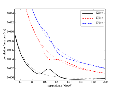
Figure 1: The correlation functions $\xi_{0}^{0}(x)$ (black solid line), $\xi_{2}^{0}(x)$ (red dashed line), and $\xi_{4}^{0}(x)$ (blue dot-dashed line) defined in Eq. (3) at the present time ($z=0$) with galaxy bias $b_{g}=1$. The dotted curves show $\xi_{n}^{m}(x)$ with the no-wiggle power spectrum given in Eisenstein & Hu (1998) to highlight the BAO bump in each curve.

We plot in Fig. 1 the three radial functions $\xi_{0}^{0}(x)$, $\xi_{2}^{0}(x)$, and $\xi_{4}^{0}(x)$. All three radial functions $\xi_{n}^{m}(x)$ show BAOs, but the BAO bumps appear at different separations for the different functions. Therefore, since the 2PCF is given for different orientations with respect to the line of sight by the linear combination of three radial functions in Eq. (2), the BAO peak location in two dimensions is anisotropic and varies with the line-of-sight angle. Examples of the anisotropies are shown in the bottom right panel of Fig. 3 and Fig. 4, respectively, for the BAO scales and for the very large scales. The bottom line is that the redshift-space distortion induces anisotropies in the location of the BAO

The purpose of this paper is to develop a heuristic understanding of these anisotropies. The second goal is to study geometrical tests of dark energy that use these two-dimensional configuration-space BAO anisotropies. Below we will explain in greater detail how the anisotropies are generated from the velocity field. With this understanding, we will be able to go beyond simply the usual distance measurements from BAO, as the shape of angular contours of the redshift-space 2PCF can be used for the broadband Alcock-Paczynski test (Song et al., 2014) and for a dynamical measure of dark energy by obtaining $f\sigma_{8}$ from Eq. (2) (Song et al., 2010, 2011; Beutler et al., 2012; Reid et al., 2012; de la Torre et al., 2013). Note that the $\sigma_{8}$ dependence comes through the amplitude of the linear matter power spectrum. Moreover, features like the zero crossing in the right-bottom corner of Fig. 4 may provide a useful probe for, e.g. matter-radiation equality (Prada et al., 2011).

The rest of this paper is organized as follows. In Sec. 2, we construct a heuristic but concrete physical model for the redshift-space 2PCF in linear theory. We show that the terms proportional to $\beta$ in Eq. (2) originate from the variation in the bulk motion of galaxies while the $\beta^{2}$ terms account for the variation in the pairwise velocity dispersion. Based on this model, we then discuss the anisotropies in the BAO bump in greater detail in Sec. 3. We conclude with a discussion of possible future research directions in Sec. 4.

2 Anisotropies in the redshift-space 2PCF

In this Section, we present a physical explanation for the anisotropies in the galaxy 2PCF. First, in Sec. 2.1, we construct from the linear growth rate and the continuity equation the peculiar-velocity field around a typical galaxy. We then calculate the redshift-space 2PCF by including the line-of-sight directional component of the peculiar velocity. Although this captures the dominant effect, this heuristic argument must be complemented by the spatial variation of the second-order moment of the velocity field in order to completely account for the the linear redshift-space distortion. In Sec. 2.2, we demonstrate this with the streaming model (Peebles, 1980; Fisher et al., 1994; Fisher, 1995; Scoccimarro, 2004) that describes the redshift-space 2PCF by convolution between the real-space 2PCF and the pairwise-velocity distribution function.

2.1 Understanding anisotropies: a heuristic argument

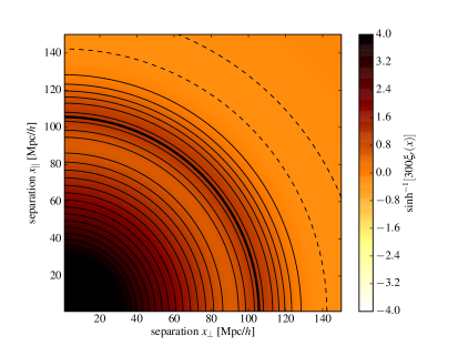
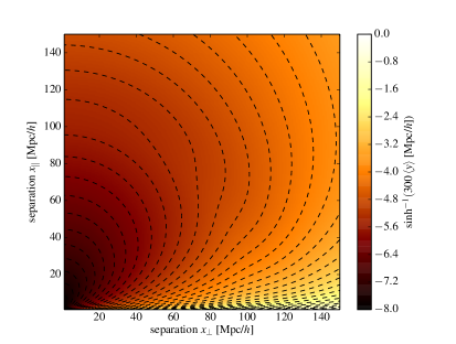
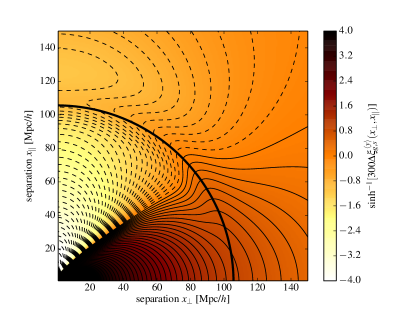
Figure 2: The two-dimensional $(x_{\perp},x_{\parallel})$ 2PCFs from the heuristic argument given in Sec. 2.1. These plots are for $b_{g}=2$ galaxies at $z=0.5$. For each plot, we show the contour lines for arc-sine-hyperbolic of the function as indicated in the label next to the colorbar. The value exceeding the colorbar range is painted as the corresponding extreme colors. Contour lines are drawn for integer multiples of $1/6$ ($1/9$ for the $\Delta\xi_{g,s}^{\left<y\right>}$), and dashed lines are for negative values. Top left: Two-dimensional contour of the real-space 2PCF. Without redshift-space distortions, the 2PCF is isotropic. We can think of the real-space 2PCF as a typical density profile around a galaxy. One can see the BAO bump around the isotropic ring with $x\approx 106~{}\mathrm{Mpc}/h$. Top right: The mean displacement $\left<y\right>$ along the LoS direction. The displacement vector is along the negative-$x_{\parallel}$ direction, and brighter (darker) colors show lower (higher) amplitudes. For a given separation, the line-of-sight direction shows larger displacement, while the displacement field itself is a decreasing function of separation. Bottom left: Correction to the apparent density profile (2PCF) due to the velocity field. The correction is given by the LoS derivative of the the line-of-sight displacement shown in the Top right panel. While the projection effect enhances the apparent clustering toward the perpendicular direction, the reduction of the displacement amplitude reduces the apparent clustering toward the parallel direction. Bottom right: Final two-dimensional density distribution (2PCF) from the heuristic argument combining the real space isotropic density distribution (2PCF) and anisotropic correction due to the scale-dependent LoS displacement.

Consider a spherically symmetric distribution of galaxies with a radial profile of number density $n_{g}(x,t)=\bar{n}_{g}(t)\left[1+\xi_{g}(x,t)\right]$, where $\xi_{g}(x)$ is the real-space galaxy 2PCF,

$$\xi_{g}(x,t)=\left<\delta_{g}(\mathbf{x}_{1},t)\delta_{g}(\mathbf{x}_{0},t)\right>,$$ (4)

where $\delta_{g}$ is the fractional galaxy density perturbation. Here, we denote the location of the central galaxy by $\mathbf{x}_{0}$, and other galaxies by $\mathbf{x}_{1}$ so that $x=|\mathbf{x}_{1}-\mathbf{x}_{0}|$. As the galaxy 2PCF measures the excess number of neighboring galaxies as a function of distance, the quantity $\bar{n}_{g}(1+\xi_{g})$ provides the mean radial profile of the galaxy density around a typical galaxy in the Universe.

In the top left panel of Fig. 2 (see also the black solid curve in Fig. 1), we show a contour plot of the radial density profile around the central galaxy (linear theory galaxy 2PCF) as a function of the parallel separation $x_{\parallel}$ and perpendicular separation $x_{\perp}$ to the line of sight. For smaller radii, the galaxy density decreases monotonically until it reaches the BAO bump around $x\approx 105~{}\mathrm{Mpc}/h$ and then decreases again after the BAO peak. At around $x\approx 150~{}\mathrm{Mpc}/h$, the density profile reaches a minimum and then increases afterwards to reach the cosmic mean in the $x\to\infty$ limit. We show the contour plot for $\sinh^{-1}(300\xi_{g})$, which scales linearly when $|\xi_{g}|<1/300$ but logarithmically for larger arguments, to represent the large dynamical range of the 2PCF.

In linear theory, the galaxy density contrast evolves in time as $\delta_{g}\equiv n_{g}(x,t)/\bar{n}_{g}(t)-1=\xi_{g}(x,t)\propto D^{2}(t)$, with the linear growth factor $D(t)$. Then, from the linear bias relation, we estimate the matter density contrast as $\delta_{m}=\delta_{g}/b_{g}$ with the linear bias parameter $b_{g}$. Once the time evolution of the matter density contrast is known, the linearized continuity equation,

$$\frac{\mathrm{d}\delta_{m}(\mathbf{x},t)}{\mathrm{d}t}+\frac{1}{a}\nabla_{\mathbf{x}}\mathbf{u}(\mathbf{x},t)=0,$$ (5)

allows us to calculate the corresponding peculiar-velocity field,

$$\mathbf{u}(\mathbf{x},t)=-2\frac{aHf}{b_{g}}\nabla_{\mathbf{x}}\left[\nabla_{\mathbf{x}}^{-2}\xi_{g}(\mathbf{x},t)\right].$$ (6)

Here, $\nabla_{\mathbf{x}}^{-2}$ is the inverse Laplacian, and we use $dD^{2}/dt=2aHfD^{2}$ with the scale factor $a$, the Hubble expansion rate $H$, and logarithmic growth factor $f\equiv\mathrm{d}\ln D/\mathrm{d}\ln a$. The right-hand side of Eq. (6) can be written as an integral, by using the Green’s function $|\mathbf{x}-\mathbf{x}^{\prime}|^{-2}$ of the three-dimensional Laplacian, as

$$\mathbf{u}(\mathbf{x},t)=-2\frac{aHf}{b_{g}}\frac{\mathbf{x}}{x^{3}}\int_{0}^{x}dy\xi_{g}(y)y^{2}.$$ (7)

To facilitate comparison to Eq. (2), we use the $\ell=1$ case of the identity [Eq. (20) in (Matsubara & Suto, 1996)],

$$\xi_{2\ell}^{0}(x_{0})=\frac{(-1)^{\ell}}{x_{0}^{2\ell+1}}\left(\prod_{i=1}^{\ell}\int_{0}^{x_{i-1}}x_{i}dx_{i}\right)x_{\ell}^{2\ell}\left(\frac{d}{dx_{\ell}}\frac{1}{x_{\ell}}\right)^{\ell}x_{\ell}\xi_{0}^{0}(x_{\ell}),$$ (8)

to rewrite the velocity field as

$$\mathbf{u}(\mathbf{x},t)=-\frac{2}{3}aHfb_{g}\left[\xi_{0}^{0}(x)+\xi_{2}^{0}(x)\right]\mathbf{x},$$ (9)

where $\xi_{n}^{m}(x)$ is defined in Eq. (3). As we are considering a spherically symmetric distribution of galaxies, the velocity field $\mathbf{u}(\mathbf{x},t)$ is purely radial and aimed at the central-galaxy location $\mathbf{x}_{0}$.

When we look at this spherical distribution of galaxies in redshift space (with line-of-sight direction $\hat{\mathbf{n}}$), galaxies at $\mathbf{x}$ appear to be at $\mathbf{x}\to\mathbf{s}=\mathbf{x}+y\hat{\mathbf{n}}$, where

$$y=\frac{\mathbf{u}\cdot\hat{\mathbf{n}}}{aH}=-\frac{2}{3}fb_{g}x_{\parallel}\left[\xi_{0}^{0}(x)+\xi_{2}^{0}(x)\right],$$ (10)

is the displacement due to the line-of-sight component of the peculiar velocity $\mathbf{u}$. We show the displacement $y$ in the top right panel of Fig. 2. Two competing effects determine the anisotropies in the displacement $y$: the amplitude of the velocity and the line-of-sight projection. For a fixed line-of-sight angle, the amplitude of the displacement is a decreasing function of $x$. For a fixed separation $x$, the line-of-sight projection of a purely radial velocity field diminishes the displacement along the perpendicular direction and maximizes it along the parallel direction. Adding up the two effects, the displacement field is smaller along the perpendicular direction and for large separations, and it has a maximum amplitude ($y$ is negative as the velocity is toward the center) along the parallel direction.

Since the total galaxy number stays the same in real and redshift space, we find the redshift-space density contrast,

$$\delta_{g,s}(\mathbf{x})= \left(1+\delta_{g}(\mathbf{x})\right)\left|\frac{\partial^{3}s}{\partial^{3}x}\right|^{-1}-1\simeq\delta_{g}(\mathbf{x})-\frac{\mathrm{d}y}{\mathrm{d}x_{\parallel}}.$$ (11)

The leading-order redshift-space distortion in peculiar velocity is therefore given by the line-of-sight derivative of the displacement, which itself is the line-of-sight projection of the peculiar velocity. This can be readily understood because constant line-of-sight velocity would only shift all galaxies by the same amount, and the density contrast only shifts up and down between real and redshift space. We work out the linear correction,

$$\frac{\mathrm{d}y}{\mathrm{d}x_{\parallel}}= -\frac{2}{3}fb_{g}\left[\xi_{0}^{0}(x)+\xi_{2}^{0}(x)\right]+2fb_{g}\mu^{2}\xi_{2}^{0}(x),$$ (12)

because $\partial x/\partial x_{\parallel}=x_{\parallel}/x=\mu$, and

$$\frac{\mathrm{d}}{\mathrm{d}x}\left[\xi_{0}^{0}(x)+\xi_{2}^{0}(x)\right]=-\frac{3}{x}\xi_{2}^{0}(x)$$ (13)

from the identities,

$$\frac{\mathrm{d}j_{\ell}(x)}{\mathrm{d}x}= \frac{\ell}{x}j_{\ell}(x)-j_{\ell+1}(x)$$

$$j_{\ell-1}(x)+j_{\ell+1}(x)= \frac{2\ell+1}{x}j_{\ell}(x).$$ (14)

The $\mu^{2}$ term in Eq. (12) accounts for the anisotropic correction due to the inflow of galaxies toward the center, which suppresses the density contrast along the parallel directions. The resulting redshift-space-density contrast is highly anisotropic: the enhancement is along the perpendicular direction and suppression along the parallel direction as shown in the bottom right panel of Fig. 2. Note that the correction term due to the bulk velocity (bottom-left panel) has a peculiar feature around BAO scales (shown with the thick black line) that anisotropically shifts the BAO peak location. We discuss the shift of the BAO peak more in Sec. 3.

Just as we construct the galaxy density distribution from the real-space 2PCF, we interpret the anisotropic density distribution in redshift space as the redshift-space 2PCF:

$$\xi_{g,s}(x,\mu)=\left[b_{g}^{2}+\frac{2}{3}fb_{g}\right]\xi_{0}^{0}(x)-\frac{4}{3}fb_{g}\xi_{2}^{0}(x)\mathcal{P}_{2}(\mu),$$ (15)

with $\mathcal{P}_{2}(\mu)=\frac{1}{2}(3\mu^{2}-1)$ the Legendre polynomial. The redshift-space 2PCF, Eq. (15), that we have derived from the heuristic argument here correctly reproduces the terms proportional to $f$ in the usual expression in Eq. (2). This argument, based on the mean streaming velocity, cannot, however, reproduce the full linear-order redshift-space distortion. We will need to include in the following Section the scale-dependent velocity dispersion to reproduce the terms proportional to $f^{2}$.

2.2 The streaming model and linear redshift space distortion

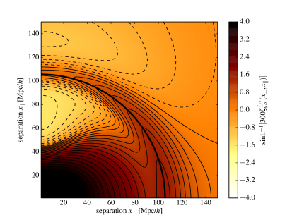
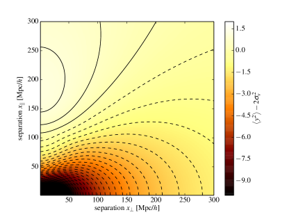
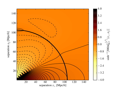
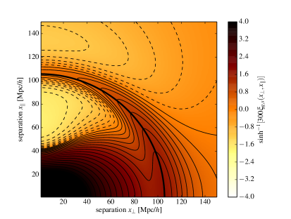
Figure 3: Two-dimensional $(x_{\perp},x_{\parallel})$ 2PCF from the streaming model. The color scheme and contour lines are the same as Fig. 2 except for the top right panel where the color scale is linear and contour lines show multiples of half-integer. Contour lines are for multiples of $1/9$ for $\Delta\xi_{g,s}^{\left<y^{2}\right>}$. Top left: Redshift-space 2PCF including only the effect from mean displacement $\xi_{g}-d/dx_{\parallel}\left<y\right>$. This plot is the same as the bottom right panel of Fig. 2. Top right: The scale and angular dependence of the second-order moment $\left<y^{2}\right>-2\sigma_{v}^{2}$ of the line-of-sight pairwise velocity field from linear theory. To show the angular dependence more clearly, we show a wider range of scales. The second moment $\left<y^{2}\right>$ asymptotes to the constant value $\left<y^{2}\right>\to 2\sigma_{v}^{2}$ for large separations ($x\to\infty$). Mostly $\left<y^{2}\right>\lesssim 2\sigma_{v}^{2}$ except along the line of sight and $x\gtrsim 100~{}\mathrm{Mpc}/h$ where $\xi_{1}^{3}(x)<\xi_{2}^{2}(x)$. Along the parallel direction, $\left<y^{2}\right>$ reaches the maximum around $x\approx 180~{}\mathrm{Mpc}/h$, and decreases to $2\sigma_{v}^{2}$. The correction to the 2PCF is given by the second derivative of the second moment. Bottom left: Correction to the redshift-space 2PCF from the second momentum of the displacement $\Delta\xi_{g,s}^{\left<y^{2}\right>}\equiv\frac{1}{2}d^{2}/dx_{\parallel}^{2}\left<y^{2}\right>$. Like the contribution from the mean displacement (the bottom left panel of Fig. 2), the anisotropic correction shows clear trend: redshift-space distortion decreases (negative correction) the correlation function along the LoS direction and increases (positive correction) along the direction perpendicular to the line of sight. However, the amplitude of the anisotropy is sub-dominant to the effect from the mean displacement. Bottom right: Redshift-space 2PCF from linear Kaiser expression Eq. (2). The contribution from the second order moments deepens the negative valley along the line-of-sight direction and increases the perpendicular directional clustering amplitude. Overall, however, the anisotropies are dominated by the mean displacement.

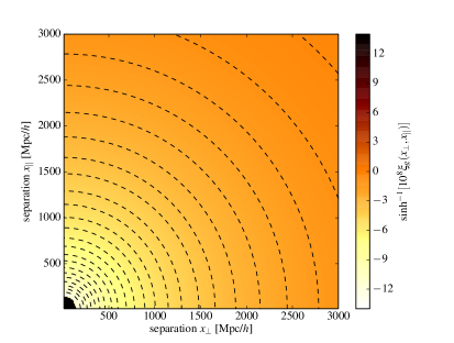
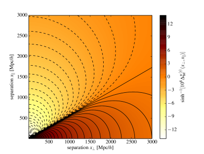
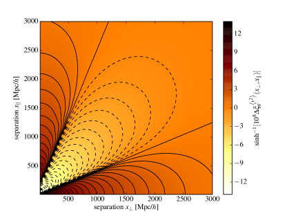
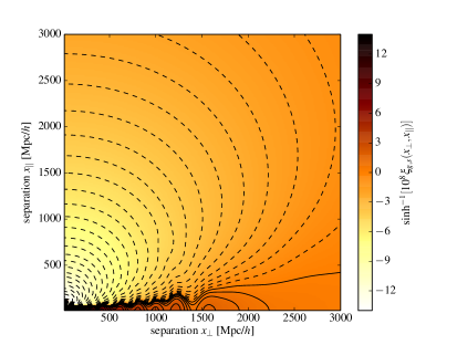
Figure 4: Two-dimensional $(x_{\perp},x_{\parallel})$ 2PCF from the streaming model for larger separations $x<3000~{}[\mathrm{Mpc}/h]$. The color scheme and contour lines are for sinh${}^{-1}(10^{8}f)$ where $f$ is the function to be shown, indicated in the label of colorbar. Top left: isotropic, real space 2PCF Top right: Correction due to the mean displacement, $\Delta\xi_{g,s}^{\left<y\right>}$ Bottom Left: Correction due to the second moment of the displacement, $\Delta\xi_{g,s}^{\left<y^{2}\right>}$ Bottom right: Redshift-space 2PCF from linear Kaiser expression, Eq. (2). Note that we have not included the wide-angle effect (Szalay et al., 1998), which must be included when the distance from the observer to the central galaxy is comparable to the perpendicular separation $x_{\perp}$.

The redshift-space distortion due to the scale-dependent variance of the line-of-sight velocity field can be best seen in the streaming model (Peebles, 1980; Fisher et al., 1994; Fisher, 1995; Scoccimarro, 2004). Here, pair conservation relates the the redshift-space 2PCF to the real-space 2PCF via coordinate mapping as

$$1+\xi_{g,s}(s_{\perp},s_{\parallel})=\int_{-\infty}^{\infty}dy\left[1+\xi_{g}(x)\right]f\left(y;\mathbf{x}\right).$$ (16)

Here, $y=s_{\parallel}-x_{\parallel}=\mathbf{v}_{12}\cdot\hat{\mathbf{n}}/(aH)$ is again the displacement ($\mathbf{v}_{12}$ is pair-weighted relative velocity, that we call pairwise velocity for short) between real space and redshift space, and $f(y;\mathbf{x})$ is the line-of-sight directional pairwise velocity distribution function, the probability distribution of the displacement $y$ at given separation $\mathbf{x}=(x_{\perp},x_{\parallel})$. As the displacement $y$ is small in linear theory, we can expand the right hand side of Eq. (16) around the position in redshift space (Fisher, 1995; Scoccimarro, 2004), and Eq. (16) becomes

$$1+\xi_{g,s}(s_{\perp},s_{\parallel})$$

$$= \left[1+\xi_{g}(s)\right]\int_{-\infty}^{\infty}dy\biggl{[}f\left(y;s_{\perp},s_{\parallel}\right)+(x_{\parallel}-s_{\parallel})\frac{d}{ds_{\parallel}}f\left(y;s_{\perp},s_{\parallel}\right)$$

$$+\frac{1}{2}(x_{\parallel}-s_{\parallel})^{2}\frac{d^{2}}{ds_{\parallel}^{2}}f\left(y;s_{\perp},s_{\parallel}\right)\biggl{]}+\mathcal{O}(\xi^{2})$$

$$= 1+\xi_{g}(x)-\frac{d}{dx_{\parallel}}\left<y\right>+\frac{1}{2}\frac{d^{2}}{dx_{\parallel}^{2}}\left<y^{2}\right>+\mathcal{O}(\xi^{2}),$$ (17)

to linear order in $\xi_{g}(x)$. Note that we pull $1+\xi_{g}(x)=1+\xi_{g}(s)+\xi_{g}^{\prime}(s)(x-s)+\mathcal{O}(\xi^{3})\simeq 1+\xi_{g}(s)$ outside the integral. The leading contributions to $\left<y\right>$ and $\left<y^{2}\right>$ are both linear in $\xi(x)$ (see Eq. (23) and Eq. (25) below for the explicit expression). Again, Eq. (17) tells us that what is relevant for the linear redshift-space distortion is the line-of-sight variation of the mean and the variance of the displacement.

We calculate the mean and the variance of the displacement in linear theory as follows. First, we calculate the displacement $y\equiv\mathbf{v}_{12}\cdot\hat{\mathbf{n}}/(aH)$ from the pairwise velocity,

$$\mathbf{v}_{12}(\mathbf{x})=\left(\mathbf{v}(\mathbf{x}_{1})-\mathbf{v}(\mathbf{x}_{0})\right)\left(1+\delta_{g}(\mathbf{x}_{1})\right)\left(1+\delta_{g}(\mathbf{x}_{0})\right),$$ (18)

whose leading-order expectation value is given by

$$\left<\mathbf{v}_{12}(\mathbf{x})\right>=\left<\mathbf{v}(\mathbf{x}_{1})\delta_{g}(\mathbf{x}_{0})\right>-\left<\mathbf{v}(\mathbf{x}_{0})\delta_{g}(\mathbf{x}_{1})\right>+\mathcal{O}(\xi^{2}).$$ (19)

Statistical homogeneity guarantees $\left<\mathbf{v}(\mathbf{x}_{0})\delta_{g}(\mathbf{x}_{0})\right>=\left<\mathbf{v}(\mathbf{x}_{1})\delta_{g}(\mathbf{x}_{1})\right>=0$. We calculate the velocity field from the Fourier transform,

$$\mathbf{v}(\mathbf{x}_{0})=aHf\int\frac{d^{3}k}{(2\pi)^{3}}\frac{i\hat{\mathbf{k}}}{k}\delta_{m}(\mathbf{k})e^{i\mathbf{k}\cdot\mathbf{x}_{0}},$$ (20)

of the continuity equation [Eq. (5)]. Then

$$\left<\mathbf{v}_{12}(\mathbf{x})\right>=2\frac{aHf}{b_{g}}\int\frac{d^{3}k}{(2\pi)^{3}}\frac{i\hat{\mathbf{k}}}{k}P_{g}(k)e^{i\mathbf{k}\cdot\mathbf{x}}=-2\frac{aHf}{b_{g}}\mathbf{x}\xi^{1}_{1}(x).$$ (21)

Here, we use the identity,

$$\int\frac{d\Omega_{k}}{4\pi}\hat{\mathbf{k}}e^{i\hat{\mathbf{k}}\cdot\mathbf{r}}=i\hat{\mathbf{r}}j_{1}(r).$$ (22)

Note that the velocity field is radial everywhere, a consequence of statistical isotropy. The mean displacement,

$$\left<y\right>=\frac{1}{aH}\left<\mathbf{v}_{12,\parallel}(\mathbf{x})\right>=-2\beta x_{\parallel}\xi_{1}^{1}(x),$$ (23)

here coincides with the result from the heuristic arguments we presented in Sec. 2.1. The reason behind this correspondence is the pair-conservation equation (Peebles, 1980),

$$\frac{\mathrm{d}(1+\xi_{g}(x))}{\mathrm{d}t}+\frac{1}{a}\nabla_{\mathbf{x}}\cdot\left<\mathbf{v}_{12}(\mathbf{x})\right>=0,$$ (24)

which enable us to interpret the pairwise velocity field as the velocity field associated with radial number density given by $n_{g}(x)\propto 1+\xi_{g}(x)$. Therefore, the heuristic argument in Sec. 2.1 correctly captures the redshift-space distortion due to the mean pairwise velocity $\left<\mathbf{v}_{12}\right>$. We show the redshift-space 2PCF including this effect of mean displacement in the top left panel of Fig. 3, which is the same as the bottom right panel of Fig. 2.

Now consider the correction due to the spatial variation of the second-order moment. The second moment $\left<y^{2}\right>$ of the displacement is given by the square of the line-of-sight component of the pairwise velocity,

$$\left<y^{2}\right>= \frac{1}{a^{2}H^{2}}\left<\mathbf{v}_{12,\parallel}^{2}(\mathbf{x})\right>$$

$$= 2\beta^{2}\hat{\mathbf{n}}^{i}\hat{\mathbf{n}}^{j}\int\frac{d^{3}k}{(2\pi)^{3}}\frac{\hat{\mathbf{k}}^{i}\hat{\mathbf{k}}^{j}}{k^{2}}P_{g}(k)\left[1-e^{i\mathbf{k}\cdot\mathbf{x}}\right]$$

$$= 2\left[\sigma_{v}^{2}-\beta^{2}\int\frac{k^{2}dk}{2\pi^{2}}\frac{P_{g}(kx)}{k^{2}}\left(\frac{j_{1}(kx)}{kx}-\mu^{2}j_{2}(kx)\right)\right]$$

$$= 2\left[\sigma_{v}^{2}-\beta^{2}x^{2}\left(\xi_{1}^{3}(x)-\mu^{2}\xi_{2}^{2}(x)\right)\right],$$ (25)

where we define the one-dimensional velocity dispersion as

$$\sigma_{v}^{2}\equiv\frac{\beta^{2}}{3}\int\frac{dk}{2\pi^{2}}P_{g}(k).$$ (26)

The anisotropies due to the second moment of the displacement are determined by $\xi_{1}^{3}(x)$ and $\xi_{2}^{2}(x)$. The top-right panel of Fig. 3 shows anisotropic contours for the second-order moment $\left<y^{2}\right>-2\sigma_{v}^{2}$ of the displacement field in the two-dimensional $(x_{\perp},x_{\parallel})$ plane. As both $\xi_{1}^{3}(x)$ and $\xi_{2}^{2}(x)$ decrease for large separations, $\left<y^{2}\right>$ asymptotes to $\left<y^{2}\right>\to 2\sigma_{v}^{2}$ for large separations $x\to\infty$, but it apparently shows scale-dependent anisotropies on smaller separations. On small scales ($x\lesssim 100~{}\mathrm{Mpc}/h$), the second-order moment becomes smaller than $2\sigma_{v}^{2}$ as $\xi_{2}^{2}(x)<\xi_{1}^{3}(x)$. For separations $x\gtrsim 100~{}\mathrm{Mpc}/h$, however, $\xi_{1}^{3}(x)<\xi_{2}^{2}(x)$, and therefore $\left<y^{2}\right>>2\sigma_{v}^{2}$ for the direction parallel to the line of sight. The velocity-dispersion contribution to the redshift-space 2PCF is given by the second derivative of the second moment,

$$\Delta\xi_{g,s}^{\left<y^{2}\right>}\equiv \frac{1}{2}\frac{\mathrm{d}^{2}}{\mathrm{d}x_{\parallel}^{2}}\left<y^{2}\right>$$

$$= \beta^{2}\left[\frac{1}{5}\xi_{0}^{0}(x)-\frac{4}{7}\xi_{2}^{0}(x)\mathcal{P}_{2}(\mu)+\frac{8}{35}\xi_{4}^{0}(x)\mathcal{P}_{4}(\mu)\right].$$ (27)

We show this correction in the bottom left panel of Fig. 3. Although smaller than the mean displacement, the basic structure of the anisotropies is the same: it enhances the 2PCF along the perpendicular direction, and suppresses it along the parallel direction.

Finally, we show the redshift-space 2PCF including both the mean and the second-moment effects of the displacement in the bottom right panel of Fig. 3. As the mean displacement dominates over the second moment, the overall structure of the anisotropies is the same as in the top left panel of the same Figure. Including the spatial variation of the second moment, however, slightly deepens the negative valley along the line of sight and increases the clustering amplitude along the parallel direction.

The anisotropic structure in the redshift-space 2PCF persists on larger scales as well. The projection of the mean displacement enhances the 2PCF along the perpendicular direction and suppresses it along the parallel direction. For large separations, however, the parallel-direction suppression from the mean displacement is somewhat reduced by the positive contribution from the variance (although the net effect is still suppression along the parallel direction). In Fig. 4, we show the redshift-space 2PCF (bottom right) for larger separations ($x<3000~{}\mathrm{Mpc}/h$) along with the real-space 2PCF (top left), the mean-displacement correction (top right), and the second-moment correction (bottom left). In order to compensate the small 2PCF amplitude at these larger separations, we show $\sinh^{-1}(10^{8}\xi_{g})$ here. We caution the readers here that the contour plot in Fig. 4 is correct only when the distance from the observer to the galaxies is much larger compared to the radial separation $x_{\perp}$. Otherwise, the plane-parallel approximation is broken down, and wide-angle effect (Szalay et al., 1998) must be included. We will present the contour plot including the wide-angle effect elsewhere (Jeong et al., 2014).

The upper-most solid curve in the bottom right panel shows the zero-crossing trajectory. Unlike the real-space 2PCF (hence the monopole 2PCF) case that the zero-crossing separation can be a proxy for the ratio between matter and radiation energy density (through matter-radiation equality redshift) (Prada et al., 2011), the zero-crossing trajectory in the two-dimensional redshift-space 2PCF may also depend on the linear-theory growth factor $f$ and the galaxy bias $b_{g}$ through Eq. (2). We defer discussion about the cosmological information contained in the zero-crossing trajectory as well as its robustness to future work. We stress, however, here that a study of the zero-crossing trajectory on large scales must include the full description of the redshift-space distortion beyond the plane-parallel approximation we employ here.

3 Redshift-space distortion of the BAO

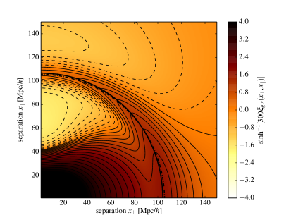
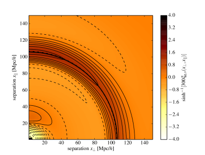
Figure 5: Location of BAO peaks in real space (dotted magenta lines) and redshift space (solid magenta lines) in the two-dimensional $(x_{\perp},x_{\parallel})$ plane. Left: BAO estimated from peak locations of the redshift-space 2PCF. Right: BAO estimated from peak locations of the redshift-space 2PCF, subtracting the anisotropic ‘background’ due to the redshift-space distortion of the no-wiggle 2PCF $\xi_{g}^{\mathrm{nw}}(x)$. We calculate the no-wiggle 2PCF from Eq. (2) with the no-wiggle power spectrum in Eisenstein & Hu (1998).

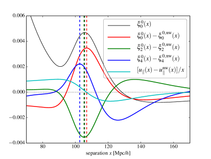
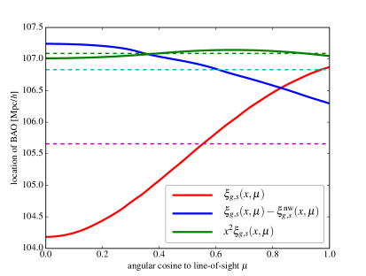
Figure 6: Left: Location of BAO peaks in the real-space galaxy 2PCF $\xi_{0}^{0}(x)$ (black) as well as the wiggly parts of $\xi_{0}^{0}(x)$, $\xi_{2}^{0}(x)$, and $\xi_{4}^{0}(x)$ which are calculated by subtracting the corresponding no-wiggle 2PCF $\xi_{n}^{m,\mathrm{nw}}(x)$. The no-wiggle $\xi_{n}^{m,\mathrm{nw}}(x)$ are calculated from Eq. (2) with the no-wiggle power spectrum in Eisenstein & Hu (1998). Vertical dotted lines show the peak locations: $r_{\mathrm{BAO}}=105.6~{}\mathrm{Mpc}/h$, $106.8~{}\mathrm{Mpc}/h$, $105.2~{}\mathrm{Mpc}/h$, and $102.6~{}\mathrm{Mpc}/h$ for, respectively, $\xi_{0}^{0}$ (black dotted), $\xi_{0}^{0}-\xi_{0}^{0,\mathrm{nw}}$ (red dotted), $\xi_{2}^{0}-\xi_{2}^{0,\mathrm{nw}}$ (green dotted), and $\xi_{4}^{0}-\xi_{4}^{0,\mathrm{nw}}$ (blue dotted). The cyan line shows the amplitude of the ‘local’ peculiar-velocity field re-scaled by $x_{\parallel}$: $[u(x)-u^{\rm nw}(x)]/x_{\parallel}$. The local velocity field vanishes around the BAO peak of $\xi_{0}^{0}(x)-\xi_{0}^{0,\rm nw}(x)$ (red solid line). Right: Location of BAO peaks as a function of the angular cosine $\mu$ to the LoS. Note that the BAO peak location depends on the method to measure the peak: red solid line and magenta dotted line are redshift-space and real space BAO peak location measured from the peak position of $\xi_{g,s}(x,\mu)$ for fixed $\mu$, while blue solid line and the cyan dotted line are the BAO peak location measured from the peak position of $\xi_{g,s}(x,\mu)-\xi_{g,s}^{\mathrm{nw}}(x,\mu)$, where $\xi_{g,s}^{\mathrm{nw}}(x,\mu)$ is the redshift-space 2PCF without the BAO bump. Green dashed line and the solid line are the same for $x^{2}\xi_{g,s}(x,\mu)$.

In the previous Section, we have shown that the anisotropies in the redshift-space 2PCF strongly depend on scale, and the linear-theory expression for the scale dependence can be explained by the line-of-sight variation in the first (mean) and the second moment of the displacement. Then, how do these anisotropies affect the baryon acoustic oscillation (BAO)?

In both Fig. 2 and Fig. 3, we show the location of the real-space BAO peak ($x\approx 106~{}\mathrm{Mpc}/h$) as an isotropic thick solid line. By comparing the real-space 2PCF (top left panel of Fig. 2) to the redshift-space 2PCF (bottom right panel of Fig. 3), we first notice that the the amplitude of the BAO bump follows the general structure of the redshift-space distortion: the BAO bump is enhanced along the perpendicular direction and suppressed along the parallel direction. We also find that the location of the local BAO ‘peak’ and the width of the BAO bump both vary, and the variation is increasingly apparent as we approach the line-of-sight direction. In this Section, we shall quantify the anisotropies in the BAO amplitude as well as shift of the BAO peak location in redshift space.

First, we study the anisotropic shift of the BAO peak in the redshift-space 2PCF. The simplest way to define the BAO peak is by finding a local maximum around the radial separation of $x\approx 105~{}\mathrm{Mpc}/h$, which is shown in the left panel of Fig. 5 as a thick solid line. In order to facilitate the comparison, we also show the quarter circle with radius of $d_{\rm BAO}$ as a thick dot-dashed line. The anisotropic shift of the BAO peaks is apparent in this plot: BAO peaks move away from the real-space location along the line-of-sight direction, and move toward the center along the perpendicular direction. We show the resulting BAO peak location in the right panel of Fig. 6 (red solid line) as a function of the angular cosine $\mu$ between the line of sight and the separation. The shift of BAO peaks due to the redshift-space distortion is biggest at each end of the parallel and perpendicular direction, and the maximum shift is about $\Delta_{\rm BAO}\approx 1.5~{}\mathrm{Mpc}/h$ compared to the real space BAO position (dashed magenta line).

While the shift is apparent for the BAO peak defined as a local maximum in the two-dimensional 2PCF, some fraction of this shift may arise from the redshift-space distortion associated with the broadband tilt of the 2PCF. In fact, the direction that the BAO peak shifts in Fig. 5 coincides with the direction to which the 2PCF correction due to redshift-space distortions increases. As discussed in Sec. 2, the redshift-space distortion suppresses the 2PCF along the line of sight and enhances it along the perpendicular direction. Also, the amount of suppression and enhancement is larger for the smaller separation. Adding these anisotropies in slope around the BAO naturally moves the peak to larger (smaller) separations along the line-of-sight (perpendicular) direction as we observe in the left panel of Fig. 5.

We can remove this shift of the BAO peak from the overall shape of the 2PCF by subtracting the broadband shape of the redshift-space 2PCF. To do so, we estimate the BAO-less broadband redshift space 2PCF from the linear redshift-space 2PCF (Eq. (2)) with the no-wiggle power spectrum in Eisenstein & Hu (1998). The right panel of Fig. 5 shows the resulting contour plot which highlights the BAO bump in the redshift-space 2PCF. Again, two thick lines show the BAO in real space (dot-dashed) and in redshift space (solid). The measured peak locations from the two-dimensional contour plot are shown in the right panel of Fig. 6 with the dashed cyan line (real space) and the solid blue line (redshift space) as a function of $\mu$. When subtracting the overall redshift-space distortion signature in the broadband 2PCF, the measured BAO peaks in redshift space are less anisotropic than before, although it is still not a perfect circle. As before, the shift of the BAO peak is greatest at each end: the parallel ($\mu=1$) and the perpendicular ($\mu=0$) directions with the maximum shift of about a third of the previous case ($\Delta_{\rm BAO}\approx 0.5~{}\mathrm{Mpc}/h$).

The shift of the BAO peak in this case can also be seen in the left panel of Fig. 6, where we plot the real-space 2PCF ($\xi_{0}^{0}(x)$, black line) along with the BAO components of $\xi_{0}^{0}(x)$ (red line), $\xi_{2}^{0}(x)$ (green line), and $\xi_{4}^{0}(x)$ (blue line). We calculate the BAO component by subtracting $\xi_{n}^{m}(x)$ from the bump-less $\xi_{n}^{m}(x)$ using the no-wiggle power spectrum in Eisenstein & Hu (1998). The vertical dashed lines show the location of peak for the lines of corresponding colors. As can be seen in the Figure, the locations of the peaks are different for all cases: $\xi_{0}^{0}(105.6~{}\mathrm{Mpc}/h)$, $\xi_{0}^{0}-\xi_{0}^{0,\mathrm{nw}}(106.8~{}\mathrm{Mpc}/h)$, $\xi_{2}^{0}-\xi_{2}^{0,\mathrm{nw}}(105.2~{}\mathrm{Mpc}/h)$, and $\xi_{4}^{0}-\xi_{4}^{0,\mathrm{nw}}(102.6~{}\mathrm{Mpc}/h)$. Since the bump in the redshift-space 2PCF is, after subtracting the broadband shape, given by a linear combination of the latter three functions with coefficients given by Eq. (2), the locations of the BAO peaks must show anisotropies.

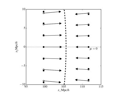
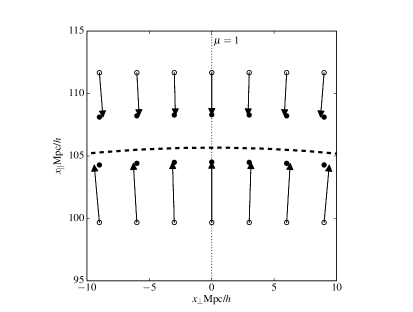
Figure 7: A sketch illustrating the shift of BAO peaks after subtracting the contribution from broadband redshift-space distortions. The left panel shows the effect around the perpendicular axis ($\mu=0$), and the right panel shows it around the parallel axis ($\mu=1$). For both cases, the peculiar-velocity field is toward the BAO peak location, represented by the thick dashed line at $d_{\rm BAO}\simeq 105~{}{\rm Mpc}/h$. The empty circles are real-space positions at constant $x_{\perp}$ (left) and $x_{\parallel}$ (right), while the filled circles are the corresponding redshift-space positions. To illustrate, we amplify the peculiar velocity by a factor of 100. For $\mu=0$ ($\mu=1$), redshift-space distortions increase the number density at larger (smaller) separation; thus, the BAO peaks shift toward larger (smaller) separation.

In Fig. 6, we notice that the estimated BAO peaks after removing the broadband shape shift to the opposite direction than the case before the removal. Why are BAO peaks shifted in this way? To understand that, let us go back to the heuristic galaxy distribution that we have considered in Sec. 2.1. In linear theory, the radial density field (set by 2PCF) is amplified by the linear growth factor, and the peculiar-velocity field is set to accommodate the growth. The overall infalling velocity field feeds the inner over-densities, and its line-of-sight projection generates the redshift-space distortion of the broadband 2PCF. Furthermore, the BAO bump in the radial profile forms a spherical shell of over-density around $x\approx 105~{}[\mathrm{Mpc}/h]$. This then generates additional velocity structure locally converging onto the peak so that the peak maintains linear growth. It is this additional local velocity field that shifts the BAO peaks even after subtracting the broadband redshift-space distortion. The local velocity field vanishes at the peak and increases its amplitude as it moves away from the peak at the vicinity of the BAO peak. Along the perpendicular direction ($\mu=0$), the sign of this additional redshift-space distortion follows the sign of the additional infalling velocity field (see Eq. (12)): it increases the 2PCF for $x\gtrsim 106~{}\mathrm{Mpc}/h$ (where $y>0$) and decreases for $x\lesssim 106~{}\mathrm{Mpc}/h$ (where $y<0$) so that the BAO peak shifts toward the larger separation. The BAO peak also shifts along the parallel direction ($\mu=1$), even though the peculiar-velocity field (cyan line in the left panel of Fig. 6) vanishes at the peak location of $\xi_{0}^{0}(x)-\xi_{0}^{0,{\rm nw}}(x)$. The asymmetry of the local peculiar-velocity field around the BAO makes the derivative of the local velocity peak at smaller $x$, around the peak of $\xi_{2}^{0}-\xi_{2}^{0,\mathrm{nw}}$ (green line in the left panel of Fig. 6). We illustrate this point in the sketch shown in Fig. 7. The shift due to the second derivative of the velocity dispersion, which is not included in the heuristic argument, further shifts the BAO to the same direction. However, the amplitude of the shift is dominated by the mean velocity.

Finally, we find that the BAO peak location detected from the volume weighted 2PCF, $x^{2}\xi(x,\mu)$, is significantly more stable than the previous two methods. The BAO location measured from $x^{2}\xi(x)$ (real space 2PCF) and from $x^{2}\xi_{g}(x,\mu)$ (redshift space 2PCF) are shown as, respectively, dashed and solid green lines in Fig. 6. In this case, we only observe sub-percent level of angular variation in the BAO peak location, because the additional factor of $x^{2}$ cancels out the BAO shift due to the radial peculiar velocity $d\left<y\right>/dx_{\parallel}$ term in Eq. (17) and the shift is mostly due to the spatial variation of the line-of-sight directional velocity dispersion. Specifically, the solution $x=x_{0}$ of the equation $[x^{2}\xi(x)]^{\prime}=0$ that defines the peak of BAO also satisfies

$$\frac{d}{dx}\left[x^{2}\frac{d\left<y\right>}{dx_{\parallel}}\right]\propto\frac{d}{dx}\left[x^{2}\left(\xi(x)-\frac{1}{x^{3}}\int_{0}^{x}dyy^{2}\xi(y)\right)\right]=0,$$ (28)

which keeps the BAO peak location constant when adding the effect of infalling bulk velocity.

In addition to the shift of the BAO peak, we also observe that after removing the broadband redshift-space distortion, the BAO bump becomes higher and sharper along the line of sight. We can understand this feature, again, from the heuristic model in Sec. 2.1: the local velocity field moves nearby galaxies close to the BAO peak, so that the BAO peak in redshift space is sharper towards the line of sight. This interesting feature was first observed by Tian et al. (2011) when they identify the BAO with a matching filter.

4 Conclusion

We present a detailed explanation for the anisotropies in the linear-theory galaxy 2PCF in redshift space. Because they are related by a non-local operation—namely, Fourier transformation—the anisotropies in the galaxy 2PCF are manifest quite differently from the anisotropies in the galaxy power spectrum. For the galaxy power spectrum, the angular dependence can be well separated from the scale dependence, and the redshift-space distortion preserves the power in the perpendicular directional. On the other hand, the angular dependence appears differently in different scales for the 2PCF, and redshift-space distortions affect the 2PCF along all directions.

To develop intuition for the anisotropic 2PCF, we consider a typical mass and galaxy distribution around a central galaxy and the associated peculiar-velocity field (via the continuity equation) that maintains the linear-theory growth of the large-scale density fluctuation. The peculiar-velocity field that feeds the growth of the over-densities around the central galaxy is radial and decreases for large separations. Then, the redshift-space distortion, proportional to the parallel derivative of the line-of-sight component of the peculiar-velocity field, enhances the galaxy 2PCF along the perpendicular direction and toward small separations. In addition to the mean peculiar velocity, we show with the streaming model that the second derivative of the second velocity moment must be included to get the $f^{2}$ terms in the linear redshift-space distortion.

We then explored with this model the anisotropic shift of BAO in the two-dimensional redshift space. Although the BAO peaks shift in the two-dimensional 2PCF, when averaging over angles, the BAO peak in the monopole 2PCF is still at the position of the real-space BAO, as the monopole 2PCF (the $\mu$-independent terms in Eq. (2)) is proportional to $\xi_{0}^{0}(x)$. Previous studies also showed that the location of the monopole BAO is robust even in the presence of non-linear redshift-space distortions. That we discover a percent-level shift of the BAO peak in redshift space, even in linear theory, however, suggests that one has to fully understand the angular-dependence in the redshift-space 2PCF including full non-linearities before using the full two-dimensional measurement of BAO for, e.g., the Alcock-Paczynski test. If naively assuming that BAO peaks are isotropic, the distance measurement using BAO will be systematically shifted.

As we have demonstrated in Sec. 3, the shift of the BAO peak depends on the method to extract the BAO peak. There are several methods to subtract the broadband shape of 2PCF and identifying BAO, and the amount of shift may depend on the method of measuring BAO peak location. For example, Tian et al. (2011) have used a Mexican-hat wavelet transformation to identify the location of BAO peaks and find that the shift of BAO is within statistical uncertainties of their Gaussian simulation. As the statistical uncertainties in that work are $\simeq 1~{}\mathrm{Mpc}/h$, in order to accommodate the need for accurate measurement of BAO in future galaxy surveys, more detailed studies, which we leave for future work, are in order. One can also reduce the shift of BAO peak by using the non-linear transform such as the log-density transformation (McCullagh et al., 2013), and future extension of this method must include the analysis for the biased tracers such as galaxies.

Finally, the galaxy 2PCF on scales larger than BAO can also be used to measure the logarithmic growth index $f$ and geometrical quantities like the angular-diameter distance $D_{A}(z)$ and Hubble expansion rate $H(z)$. On such large scales, the density field is linear, but one needs to include the correction to the usual Kaiser formula due to the curvature of the sky, radial evolution of cosmological parameters and galaxy number density, and general-relativistic corrections. We shall present the full two-dimensional 2PCF including all of these effects elsewhere (Jeong et al., 2014).

References

- Ade et al. (2013) Ade P. A. R., et al., 2013, arXiv:1303.5062
- Anderson et al. (2012) Anderson L., et al., 2012, MNRAS, 427, 3435
- Anderson et al. (2014) Anderson L., et al., 2014, MNRAS, 441, 24
- Aonley et al. (2011) Aonley A., et al., 2011, ApJS, 192, 1
- Bennett et al. (2013) Bennett C. L., et al., 2013, ApJS, 208, 20
- Beutler et al. (2011) Beutler F., et al., 2011, MNRAS, 416, 3017
- Beutler et al. (2012) Beutler F., et al., 2012, MNRAS, 423, 3430
- Blake et al. (2011a) Blake C., et al., 2011a, MNRAS, 418, 1707
- Blake et al. (2011b) Blake C., et al., 2011b, MNRAS, 415, 2892
- Busca et al. (2013) Busca N. G., et al., 2013, A&A, 552, A96
- Cole et al. (2005) Cole S., et al., 2005, MNRAS, 362, 505
- de la Torre et al. (2013) de la Torre S., et al., 2013, A&A, 557, A54
- Eisenstein et al. (2005) Eisenstein D. J., et al., 2005, ApJ, 633, 560
- Eisenstein & Hu (1998) Eisenstein D. J., Hu W., 1998, ApJ, 496, 605
- Fang et al. (2011) Fang W., Hui L., Ménard B., May M., Scranton R., 2011, PRD, 84, 063012
- Fisher (1995) Fisher K. B., 1995, ApJ, 448, 494
- Fisher et al. (1994) Fisher K. B., Davis M., Strauss M. A., Yahil A., Huchra J. P., 1994, MNRAS, 267, 927
- Freedman et al. (2012) Freedman W. L., Madore B. F., Scowcroft V., Burns C., Monson A., Persson S. E., Seibert M., Rigby J., 2012, ApJ, 758, 24
- Hamilton (1992) Hamilton A. J. S., 1992, ApJ, 385, L5
- Hamilton (1997) Hamilton A. J. S., 1997, astro-ph/9708102
- Jeong et al. (2014) Jeong D., Liang D., Kamionkowski M., 2014, in preparation
- Kazin et al. (2010) Kazin E. A., et al., 2010, ApJ, 710, 1444
- Kazin et al. (2013) Kazin E. A., et al., 2013, MNRAS, 435, 64
- Kazin et al. (2012) Kazin E. A., Sánchez A. G., Blanton M. R., 2012, MNRAS, 419, 3223
- Martínez et al. (2009) Martínez V. J., et al., 2009, ApJ, 696, L93
- Matsubara & Suto (1996) Matsubara T., Suto Y., 1996, ApJ, 470, L1
- McCullagh et al. (2013) McCullagh N., Neyrinck M. C., Szapudi I., Szalay A. S., 2013, ApJ, 763, L14
- Padmanabhan et al. (2012) Padmanabhan N., et al., 2012, MNRAS, 427, 2132
- Padmanabhan & White (2008) Padmanabhan N., White M., 2008, PRD, 77, 123540
- Peebles (1980) Peebles P. J. E., 1980, The large-scale structure of the universe. Princeton University Press
- Percival et al. (2007) Percival W. J., et al., 2007, MNRAS, 381, 1053
- Percival et al. (2010) Percival W. J., et al., 2010, MNRAS, 401, 2148
- Prada et al. (2011) Prada F., Klypin A., Yepes G., Nuza S. E., Gottloeber S., 2011, arXiv:1111.2889
- Pritchard et al. (2007) Pritchard J. R., Furlanetto S. R., Kamionkowski M., 2007, MNRAS, 374, 159
- Reid et al. (2012) Reid B. A., et al., 2012, MNRAS, 426, 2719
- Riess et al. (2011) Riess A. G., et al., 2011, ApJ, 730, 119
- Scoccimarro (2004) Scoccimarro R., 2004, PRD, 70, 083007
- Seo & Eisenstein (2007) Seo H.-J., Eisenstein D. J., 2007, ApJ, 665, 14
- Seo et al. (2010) Seo H.-J., et al., 2010, ApJ, 720, 1650
- Slosar et al. (2013) Slosar A., et al., 2013, JCAP, 4, 26
- Song et al. (2014) Song Y.-S., Okumura T., Taruya A., 2014, PRD, 89, 103541
- Song et al. (2011) Song Y.-S., Sabiu C. G., Kayo I., Nichol R. C., 2011, JCAP, 5, 20
- Song et al. (2010) Song Y.-S., Sabiu C. G., Nichol R. C., Miller C. J., 2010, JCAP, 1, 25
- Suzuki et al. (2012) Suzuki N., et al., 2012, ApJ, 746, 85
- Szalay et al. (1998) Szalay A. S., Matsubara T., Landy S. D., 1998, ApJ, 498, L1
- Tian et al. (2011) Tian H., Neyrinck M. C., Budavari T., Szalay A. S., 2011, ApJ, 728, 34
- Weinberg et al. (2013) Weinberg D. H., Mortonson M. J., Eisenstein D. J., Hirata C., Riess A. G., Rozo E., 2013, Physics Reports, 530, 87
- Xu et al. (2012) Xu X., Padmanabhan N., Eisenstein D. J., Mehta K. T., Cuesta A. J., 2012, MNRAS, 427, 2146
- Zheng et al. (2011) Zheng Z., Cen R., Trac H., Miralda-Escudé J., 2011, ApJ, 726, 38