On a nonlinear model for tumor growth in a cellular medium

Donatella Donatelli
Departement of Engineering Computer Science and Mathematics
University of L’Aquila
67100 L’Aquila, Italy.
donatella.donatelli@univaq.it univaq.it/~donatell
 and  Konstantina Trivisa
Department of Mathematics
University of Maryland
College Park, MD 20742-4015, USA.
trivisa@math.umd.edu math.umd.edu/~trivisa
Abstract.

We investigate the dynamics of a nonlinear model for tumor growth within a cellular medium. In this setting the “tumor” is viewed as a multiphase flow consisting of cancerous cells in either proliferating phase or quiescent phase and a collection of cells accounting for the “waste” and/or dead cells in the presence of a nutrient. Here, the tumor is thought of as a growing continuum $\Omega$ with boundary $\partial\Omega$ both of which evolve in time. The key characteristic of the present model is that the total density of cancerous cells is allowed to vary, which is often the case within cellular media. We refer the reader to the articles [13], [18] where compressible type tumor growth models are investigated. Global-in-time weak solutions are obtained using an approach based on penalization of the boundary behavior, diffusion, viscosity and pressure in the weak formulation, as well as convergence and compactness arguments in the spirit of Lions [19] (see also [14, 11]).

Key words and phrases:
Tumor growth models, cancer progression, mixed models, moving domain, penalization, existence.
2010 Mathematics Subject Classification:
Primary: 35Q30, 76N10; Secondary: 46E35.

1. Introduction

We investigate the dynamics of a nonlinear model for tumor growth within a cellular medium. In this setting the “tumor” is viewed as a multiphase flow consisting of cancerous cells in either proliferating phase or quiescent phase and a collection of cells accounting for the “waste” or dead cells in the presence of a nutrient (oxygen). Here, the tumor is thought of as a growing continuum $\Omega$ with boundary $\partial\Omega$ both of which evolve in time. The key characteristic of the present model is that the total density of cancerous cells is allowed to vary. We refer the reader to the articles by Enault [13], where the compressibility effect of the healthy tissue on the invasiveness of a tumor is investigated and to Li and Lowengrub [18] for references on related models.

This work focuses on major cells such as cancer cells and dead cells (or waste) in the presence of a nutrient. Motivated by the experiments of Roda et al. (2011, 2012) and the mathematical analysis in Bresch et al. [2], Friedman [17], Chen-Friedman [7], Zhao [25] and Donatelli-Trivisa [11] our model is based on the following biological principles:

  1. [a-1]

    Cancer cells are either in a proliferating phase or in a quiescent phase.

  2. [a-2]

    Proliferating cells die as a result of apoptosis which is a cell-loss mechanism.

  3. [a-3]

    Quiescent cells die in part due to apoptosis but more often due to starvation.

  4. [a-4]

    Cells change from quiescent phase into proliferating phase at a rate which increases with the nutrient level, and they die at a rate which increases as the level of nutrient decreases.

  5. [a-5]

    Proliferating cells, die at a rate which increases as the level of nutrient decreases.

  6. [a-6]

    Proliferating cells become quiescent at a rate which increases as the nutrient concentration decreases. The proliferation rate increases with the nutrient concentration.

  7. [a-7]

    The total number of cancerous cells can vary as a function of space and time accounting for the case of cancer research investigation within a cellular medium.

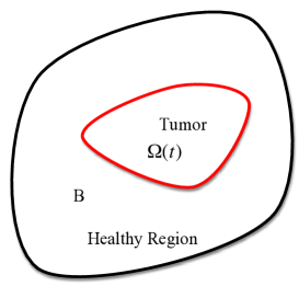
The system is given by a multi-phase flow model and the tumor is described as a growing continuum $\Omega(t)$ with boundary $\partial\Omega(t)$, both of which evolve in time.

The tumor region $\Omega_{t}:=\Omega(t)$ is contained in a fixed domain $B$ and the region $B\setminus\Omega_{t}$ represents the healthy tissue (see Figure 1).

Refer to caption
Figure 1. Healthy tissue - Tumor regime.

1.1. Description of the model

Our aim is to describe the evolution in time of the density (number of cells per unit volume) of few cellular species. Mathematical models describing continuum cell populations and their evolution typically consider the interactions between the cell number density and one or more chemical species that provide nutrients or influence the cell cycle events of a tumor cell population. In order to obtain the equations giving the evolution of cellular densities, we use the mass-balance principle for every specie,

$$\partial_{t}\varrho+\nabla\cdot(\varrho{{\bm{v}}})={\bm{G}},$$

where $\varrho$ may represent densities of cancer cells and dead cells (waste) within the tumor. The function $G$ includes in general proliferation, apoptosis or clearance of cells, and chemotaxis terms as appropriate.

Cancer cells are of two types: proliferative cells with density $P(x,t)$ and quiescent cells with density $Q(x,t).$ What is here referred as dead cells with density $D(x,t)$ includes also what is known in the theory of tumor growth as the waste or extra-cellular medium. These different populations of cells are in the presence of a nutrient (oxygen) with density $C.$ The rates of change from one phase to another are functions of the nutrient concentration C:

$\displaystyle P\to Q\,\,\mbox{at rate}\,\,K_{Q}(C),$
$\displaystyle Q\to P\,\,\mbox{at rate}\,\,K_{P}(C),$
$\displaystyle P\to D\,\,\mbox{at rate}\,\,K_{A}(C),$
$\displaystyle Q\to D\,\,\mbox{at rate}\,\,K_{D}(C),$

where $K_{Q}(C)$ denotes the rate by which proliferating cells change into quiescent cells, $K_{P}(C)$ denotes the rate by which quiescent cells change into proliferating cells, $K_{A}(C)$ stands for apoptosis, $K_{D}(C)$ denotes the rate by which quiescent cells die. Finally, dead cells are removed at rate $K_{R}$ (independent of $C$), and the rate of cell proliferation (new births) is $K_{B}$ (see (LABEL:G)).

The total density of the mixture is denoted by $\varrho_{f}$ and is given by

$$\varrho=\varrho(x,t)=[P+Q+D](x,t).$$ (1.1)

Biologically that means the total density of cancerous cells may vary which is the case when the waste produced by death of any kind does not necessarily remain within the extra cellular medium.

1.2. The velocity of the tumor

The present work considers the mechanical interactions between the various tumor cells in order to see how the mechanical properties of the tumor, and the tissue in which the tumor grows, influence tumor growth. The tumor velocity ${\bm{v}}$ reflects the continuous motion within the tumor region typically due to proliferation and removal of cells and is here given by an alternative to Darcy’s Law known in the porous medium literature as Forchheimer’s equation

$$\partial_{t}(\varrho{\bm{v}})+\operatorname{div}(\varrho{\bm{v}}\otimes{\bm{v}})+\nabla\sigma(P,Q,D)=\mu\Delta{\bm{v}}-\frac{\mu}{K}{\bm{v}},$$ (1.2)

where $\mu$ is a positive constant describing the viscous-like properties of tumor cells, $K$ denotes the permeability, and $\sigma$ denotes the pressure given by,

$$\sigma(P,Q,D)=P^{m}+Q^{m}+D^{m},\,\,\,m>\frac{3}{2}.$$ (1.3)

Equation (1.2) can be interpreted as follows. The tumor tissue is in this setting “fluid-like” and the tumor cells “flow” through the cellular medium like a fluid flows through a porous medium, obeying Forchheimer’s law. More specifically,

  • The second term on the right-hand side of (1.2) is the usual Darcy’s law, and in the present setting results from the friction of the tumor cells with the extracellular matrix.

  • The first term of the right-hand side, is a dissipative force density and results from the internal cell friction due to cell volume changes.

  • The present work takes into consideration the variation of the cell densities and velocity variations within the cellular medium which are often considered negligible in biological settings but are rather substantial in some regimes of interest.

1.3. Equations for the populations of cells

The mass conservation laws for the densities of the proliferative cells $P,$ quiescent cells $Q$ and dead cells $D$ take the following form:

$\displaystyle\partial_{t}P+\operatorname{div}(P{\bm{v}})={\bm{G_{P}}},$ (1.4)
$\displaystyle\partial_{t}Q+\operatorname{div}(Q{\bm{v}})={\bm{G_{Q}}},$ (1.5)
$\displaystyle\partial_{t}D+\operatorname{div}(D{\bm{v}})={\bm{G_{D}}}.$ (1.6)

Following Friedman [17], the source terms ${\bf\{G_{P},G_{Q},G_{D}\}}$ are of the form

$$\begin{split}&{\bm{G_{P}}}=\left(K_{B}C-K_{Q}(\bar{C}-C)-K_{A}(\bar{C}-C)\right)P+K_{P}CQ\\ &{\bm{G_{Q}}}=K_{Q}(\bar{C}-C)P-\left(K_{P}C+K_{D}(\bar{C}-C)\right)Q\\ &{\bm{G_{D}}}=K_{A}(\bar{C}-C)P+K_{D}(\bar{C}-C)Q-K_{R}D,\end{split}$$

where $C$ is the nutrient concentration.

Without loss of generality (cf. [2] and the references therein) we consider here ${\bf\{G_{P},G_{Q},G_{D}\}}$ in the following simplified version:

$$\begin{split}&{\bm{G_{P}}}=\left(K_{B}C-K_{Q}(\bar{C}-C)-K_{A}(\bar{C}-C)\right)P\\ &{\bm{G_{Q}}}=-\left(K_{P}C+K_{D}(\bar{C}-C)\right)Q\\ &{\bm{G_{D}}}=-K_{R}D.\end{split}$$ (1.7)

1.4. A linear diffusion equation for the nutrient concentration

Unlike tumor cells the density of the nutrient (oxygen) obeys a linear diffusion equation. It is well known that tumor cells consume nutrients, which diffuse into the tumor tissue from the surrounding tissue (cf. [23]). The nutrient concentration $C$ satisfies a linear diffusion equation of the form

$$\frac{\partial C}{\partial t}=D_{1}\Delta C-\left(K_{1}K_{P}CP+K_{2}K_{Q}(\bar{C}-C)Q\right)C.$$

and for simplicity, we take (see [17]) ,

$$\frac{\partial C}{\partial t}=\nu\Delta C-K_{C}C,$$ (1.8)

where $\nu>0$ is a diffusion coefficient and without loss of generality we consider $K_{C}=1$. We refer the reader also to [2], where a stationary (elliptic) equation was introduced referring to the case when the diffusion time-scale of the oxygen is much lower than the time scale of cellular division. The present setting takes into consideration the dynamic aspects of the diffusion.

Adding (1.4)-(1.6) and taking into consideration (1.1) and (LABEL:G) we arrive at the following transport relation for the evolution of the total density of the mixture

$\displaystyle\partial_{t}\varrho+\operatorname{div}(\varrho{\bm{v}})=$ $\displaystyle{\bm{G_{P}}}+{\bm{G_{Q}}}+{\bm{G_{D}}}$
$\displaystyle=$ $\displaystyle(K_{A}+K_{B}+K_{Q})CP-(K_{A}+K_{Q})\bar{C}P$
$\displaystyle-K_{D}\bar{C}Q+(K_{D}-{K_{P}})CQ-K_{R}D.$ (1.9)

Our aim is to study the system (1.2)-(1.8) in a spatial domain $\Omega_{t}$, with a boundary $\Gamma=\partial\Omega_{t}$ varying in time.

1.5. Boundary behavior

The boundary of the domain $\Omega_{t}$ occupied by the tumor is described by means of a given velocity ${\bm{V}}(t,{\bm{x}}),$ where $t\geq 0$ and ${\bm{x}}\in\mathbb{R}^{3}.$ More precisely, assuming ${\bm{V}}$ is regular, we solve the associated system of differential equations

$$\frac{d}{dt}{\bm{X}}(t,{\bm{x}})={\bm{V}}(t,{\bm{X}}),\,\,t>0,\,\,{\bm{X}}(0,{\bm{x}})={\bm{x}},$$

and set

$$\begin{cases}\!\!\!\!&\Omega_{\tau}={\bm{X}}(\tau,\Omega_{0}),\,\,\mbox{where}\,\,\Omega_{0}\subset\mathbb{R}^{3}\,\,\mbox{is a given domain,}\\ \!\!\!\!&\Gamma_{\tau}=\partial\Omega_{\tau},\,\,\mbox{and}\,\,Q_{\tau}=\left\{(t,x)|t\in(0,\tau),x\in\Omega_{\tau}\right\}.\end{cases}$$

The model is closed by giving boundary conditions on the (moving) tumor boundary $\Gamma_{\tau}.$ More precisely, we assume that the boundary $\Gamma_{\tau}$ is impermeable, meaning

$$({\bm{v}}-{\bm{V}})\cdot{\bm{n}}|_{\Gamma_{\tau}}=0,\,\,\mbox{for any}\,\,\tau\geq 0.$$ (1.10)

In addition, for viscous fluids, Navier proposed the boundary condition of the form

$$[\mathbb{S}{\bm{n}}]_{\mbox{tan}}|_{\Gamma_{\tau}}=0,$$ (1.11)

with $\mathbb{S}$ denoting the viscous stress tensor which in this context is assumed to be determined through Newton’s rheological law

$$\mathbb{S}=\mu\Big{(}\nabla{\bm{v}}+\nabla^{\perp}{\bm{v}}-{2\over 3}\operatorname{div}{\bm{v}}\mathbb{I}\Big{)}+\xi\operatorname{div}{\bm{v}}\mathbb{I}.$$

The constants $\mu>0$, $\xi\geq 0$ are respectively the shear and bulk viscosity coefficients. Condition (1.11) namely says that the tangential component of the normal viscous stress vanishes on $\Gamma_{\tau}.$ The concentration of the nutrient on the boundary satisfies the condition:

$$C|_{\Gamma_{t}}=0.$$ (1.12)

Finally, the problem (1.4)-(1.12) is supplemented by the initial conditions

$$\begin{split}P(0,\cdot)=P_{0},\quad Q(0,\cdot)=Q_{0},\quad D(0,\cdot)=D_{0},\\ C(0,\cdot)=C_{0}\leq\bar{C},\quad{\bm{v}}(0,\cdot)={\bm{v}}_{0}\ \qquad\quad\text{in $\Omega_{0}$.}\end{split}$$ (1.13)

Our main goal is to show the existence of global in time weak solutions to (1.2)-(1.13) for any finite energy initial data. Related works on the mathematical analysis of cancer models have been presented by Friedman et al. [17], [7] who established the local existence of radial symmetric smooth solutions to a related model. The analysis in [25] treated a parabolic-hyperbolic free boundary problem and provided a unique global solution in the radially symmetric case. In the forth mentioned articles the tumor tissue is assumed to be a fluid flowing a porous medium and the velocity field is determined by Darcy’s Law

$${\bm{v}}=-\nabla_{x}\sigma\,\,\mbox{in}\,\,\Omega(t).$$

In [11] Donatelli and Trivisa obtained the global existence of weak solutions to a nonlinear model for tumor growth in a general domain $\Omega_{t}\subset\mathbb{R}^{3}$ without any kind of symmetry assumptions. The article [11] treated the tumor tissue as a fluid flowing in a porous medium with the velocity field given by Brinkman’s equation

$$\nabla\sigma=-\frac{\mu}{K}{\bm{v}}+\mu\Delta{\bm{v}},$$

and focused on the case of constant total density of cancerous cells. In [12], the same authors treat a related nonlinear model and discuss the effect of drug application on tumor growth.

The main contribution of the present article to the existing theory can be characterized as follows:

  • The present work treats the tumor as a mixture with a variable total density of cancerous cells. In accordance, the velocity of the tumor verifies an extension of Darcy’s law known as Forchheimer’s equation obtained by analogy to the Navier-Stokes equation. The global existence of weak solutions within a moving domain in $\mathbb{R}^{3}$ is obtained without assuming any kind of symmetry. For related works involving compressible-type models for the investigation of tumor growth models we refer the reader to Enault [13], Li and Lowengrub [18] and the references therein.

  • The framework presented here relies on biologically grounded principles [a-1]-[a-7], which are motivated by experiments performed by Roda et al. [21] [8], [22] and provide a description of the dynamics of the population of cells within the tumor.

We establish the global existence of weak solutions to (1.2)-(1.13) on time dependent domains, supplemented with slip boundary conditions. The existence theory for the barotropic Navier-Stokes system on fixed spatial domains in the framework of weak solutions was developed in the seminal work of Lions [19].

The main ingredients of our approach can be formulated as follows:

  • In the construction of a suitable approximating scheme the penalizations of the boundary behavior, diffusion and viscosity are introduced in the weak formulation. A penalty approach to slip conditions for stationary incompressible flow was proposed by Stokes and Carey [24] (see also [11, 16]). In the present setting, the variational (weak) formulation of the Forchheimer’s equation is supplemented by a singular forcing term

    $$\frac{1}{\varepsilon}\int_{\Gamma_{t}}({\bm{v}}-{\bm{V}})\cdot{\bf n}{\bm{\varphi}}\cdot{\bm{n}}dS_{x},\,\,\,\varepsilon>0\,\,\mbox{small},$$ (1.14)

    penalizing the normal component of the velocity on the boundary of the tumor domain.

  • In addition to (1.14), we introduce a variable shear viscosity coefficient $\mu=\mu_{\omega},$ as well as a variable diffusion $\nu=\nu_{\omega}$ with $\mu_{\omega},\nu_{\omega}$ vanishing outside the tumor domain and remaining positive within the tumor domain, to accommodate the time-dependent nature of the boundary.

  • In constructing the approximating problem we employ a number of regularizations/penalizations: $\eta,\varepsilon,\delta,\omega$. Keeping $\eta,\varepsilon,\delta,\omega$ fixed, we solve the modified problem in a (bounded) reference domain $B\subset\mathbb{R}^{3}$ chosen in such way that

    $$\bar{\Omega}_{\tau}\subset B\,\,\mbox{for any}\,\,\tau\geq 0.$$

    Letting $\eta\to 0$ we obtain the solution $(P,Q,D)_{\delta,\omega,\varepsilon}$ within the fixed reference domain.

  • We take the initial densities $(P_{0},Q_{0},D_{0})$ vanishing outside $\Omega_{0},$ and letting the penalization $\varepsilon\to 0$ for fixed $\omega>0$ we obtain a “two-phase” model consisting of the tumor region and the healthy tissue separated by impermeable boundary. We show that the densities vanish in part of the reference domain, specifically on $((0,T)\times B)\setminus Q_{T}.$

  • We let first the penalization $\varepsilon$ vanish and next we perform the limit $\omega\to 0$ and $\delta\to 0.$

  • The slip boundary conditions considered here are suitable in the context of moving domains and biologically relevant as confirmed by experimental evidence.

The paper is organized as follows: Section 1 presents the motivation, modeling and introduces the necessary preliminary material. Section 2 provides a weak formulation of the problem and states the main result. Section 3 is devoted to the penalization problem and to the construction of a suitable approximating scheme. In Section 4 we present the modified energy inequality and collect all the uniform bounds satisfied by the solution of the approximating scheme. In Section 5, we derive essential pressure estimates. In Section 6 the singular limits for $\varepsilon\to 0$ is performed. The key ingredient at this step is the establishment of the strong convergence of the density, which is obtained, in analogy to the theory of compressible Navier-Stokes equation, by establishing the weak continuity of the effective viscous pressure. Subsequently it is proven that in fact the proliferating, quiescent, dead cells and the nutrient are vanishing in the healthy tissue. In Sections 7 and 8 the singular limits $\omega\to 0$ and $\delta\to 0$ are performed successively.

2. Weak formulation and main results

Definition 2.1.

We say that $(P,Q,D,{\bm{v}},C)$ is a weak solution of problem (1.4)-(1.13) supplemented with boundary data satisfying (1.10)-(1.12) and initial data $(P_{0},Q_{0},D_{0},{\bm{v}}_{0},C_{0})$ satisfying (1.13) provided that the following hold:

$\bullet$ $(P,Q,D)\geq 0$ represents a weak solution of (1.4)-(1.5)-(1.6) on $[0,T]\times\Omega_{\tau}$, i.e., for any test function $\varphi\in C^{\infty}_{c}([0,T]\times\mathbb{R}^{3}),T>0$, for any $\tau\in[0,T]$ the following integral relations hold

$$\left.\begin{array}[]{l}\displaystyle{\int_{\Omega_{\tau}}P\varphi(\tau,\cdot)\,dx-\int_{\Omega_{0}}P_{0}\varphi(0,\cdot)dx=}\\ \hskip 42.67912pt\displaystyle{\int_{0}^{\tau}\!\!\int_{\Omega_{t}}\left(P\partial_{t}\varphi+P{\bm{v}}\cdot\nabla_{x}\varphi+{\bm{G_{P}}}\varphi(t,\cdot)\right)dxdt},\\ \\ \displaystyle{\int_{\Omega_{\tau}}Q\varphi(\tau,\cdot)\,dx-\int_{\Omega_{0}}Q_{0}\varphi(0,\cdot)dx}=\\ \hskip 42.67912pt\displaystyle{\int_{0}^{\tau}\!\!\int_{\Omega_{t}}\left(Q\partial_{t}\varphi+P{\bm{v}}\cdot\nabla_{x}\varphi+{\bm{G_{Q}}}\varphi(t,\cdot)\right)dxdt,}\\ \\ \displaystyle{\int_{\Omega_{\tau}}D\varphi(\tau,\cdot)\,dx-\int_{\Omega_{0}}D_{0}\varphi(0,\cdot)dx=}\\ \hskip 42.67912pt\displaystyle{\int_{0}^{\tau}\!\!\int_{\Omega_{t}}\left(D\partial_{t}\varphi+D{\bm{v}}\cdot\nabla_{x}\varphi+{\bm{G_{D}}}\varphi(t,\cdot)\right)dxdt}.\end{array}\right\}$$ (2.1)

In particular,

$$P\in L^{\infty}([0,T];L^{m}(\Omega_{\tau})),\,\,Q\in L^{\infty}([0,T];L^{m}(\Omega_{\tau})),\,\,D\in L^{\infty}([0,T];L^{m}(\Omega_{\tau})).$$

We remark that in the weak formulation, it is convenient that the equations (1.4)-(1.6) hold in the whole space $\mathbb{R}^{3}$ provided that the densities $P,Q,D$ are extended to be zero outside the tumor domain.

$\bullet$ Forchheimer’s equation (1.2) holds in the sense of distributions, i.e., for any test function ${\bm{\varphi}}\in C^{\infty}_{c}(\mathbb{R}^{3};\mathbb{R}^{3})$ satisfying

$${\bm{\varphi}}\cdot{\bm{n}}|_{\Gamma_{\tau}}=0\,\,\mbox{for any}\,\,\tau\in[0,T],$$

the following integral relation holds

$$\begin{split}\int_{\Omega_{\tau}}\varrho{\bm{v}}\cdot{\bm{\varphi}}(\tau,\cdot)dx&-\int_{\Omega_{0}}{(\varrho{\bm{v}})_{0}\cdot{\bm{\varphi}}(0,\cdot)dx}\\ =\int_{0}^{\tau}\!\!\int_{\Omega_{\tau}}&\Big{(}\varrho{\bm{v}}\cdot\partial_{t}{\bm{\varphi}}+\varrho{\bm{v}}\otimes{\bm{v}}:\nabla_{x}{\bm{\varphi}}\\ &+\sigma(P,Q,D)\operatorname{div}{\bm{\varphi}}-\mu\nabla_{x}{\bm{v}}:\nabla_{x}{\bm{\varphi}}-\frac{\mu}{K}{\bm{v}}{\bm{\varphi}}\Big{)}dxdt\end{split}$$ (2.2)

The impermeability boundary condition (1.10) is satisfied in the sense of traces, namely

$${\bm{v}}\in L^{2}([0,T];W^{1,2}(\mathbb{R}^{3};\mathbb{R}^{3})),$$

and

$$({\bm{v-V}})\cdot{\bm{n}}(\tau,\cdot)|_{\Gamma_{\tau}}=0\,\,\mbox{for a.a.}\,\,\tau\in[0,T].$$

$\bullet$ $C\geq 0$ is a weak solution of (1.8), i.e., for any test function $\varphi\in C^{\infty}_{c}([0,T)\times\mathbb{R}^{3}),T>0$, for any $\tau\in[0,T]$ the following integral relations hold

$$\begin{split}\int_{\Omega_{\tau}}&C\varphi(\tau,\cdot)\,dx-\int_{\Omega_{0}}C_{0}\varphi(0,\cdot)dx\\ &=\int_{0}^{\tau}\!\!\int_{\Omega_{t}}\left(C\partial_{t}\varphi-\nu\nabla_{x}C\cdot\nabla_{x}\varphi-C\varphi\right)dxdt.\end{split}$$ (2.3)

The main result of the article now follows.

Theorem 2.2.

Let $\Omega_{0}\subset\mathbb{R}^{3}$ be a bounded domain of class $C^{2+\nu}$ and let

$${\bm{V}}\in C^{1}([0,T];C^{3}_{c}(\mathbb{R}^{3};\mathbb{R}^{3}))$$

be given. Let the initial data satisfy

$$P_{0}\in L^{m}(\mathbb{R}^{3}),\,\,Q_{0}\in L^{m}(\mathbb{R}^{3}),\,\,D_{0}\in L^{m}(\mathbb{R}^{3}),\,\,C_{0}\in L^{m}(\mathbb{R}^{3}),$$
$$(P_{0},Q_{0},D_{0},C_{0})\geq 0,\,\,\,(P_{0},Q_{0},D_{0},C_{0})\not\equiv 0,\,\,\,(P_{0},Q_{0},D_{0},C_{0})|_{\mathbb{R}^{3}\setminus\Omega_{0}}=0$$

for a certain $\displaystyle{m>\frac{3}{2}}.$ Denoting by $\varrho$ the total density of cells, namely

$$\varrho(x,t)=[P+Q+D](x,t)$$

we require that

$$(\varrho{\bm{v}})_{0}=0\,\,a.a.\,on\,\,\{\varrho_{0}=0\},\,\,\int_{\Omega_{0}}\frac{1}{\varrho_{0}}|(\varrho{\bm{v}})_{0}|^{2}{\rm d}x<\infty.$$

Then the problem (1.4)-(1.8) with initial data (1.13) and boundary data (1.10), (1.11) and (1.12) admits a weak solution in the sense specified in Definition 2.1.

3. Approximating Scheme

In the heart of the approximating procedure presented here lie the so-called generalized penalty methods, which entail treating the boundary condition as a weakly enforced constraint. This approach has appeared to be suitable for treating partial slip, free surface, contact and related boundary conditions in viscous flow analysis and simulations. In incompressible viscous flow modeling such approach provides penalty enforcement of the incompressibility constraint on the velocity field [4], [5],[6].

The form of boundary penalty approximation introduced here has its origin in Courant [9]. A penalty approach to slip conditions for stationary incompressible fluids was proposed by Stokes and Carey [24]. Compressible fluid flows in time dependent domains, supplemented with the no-slip boundary conditions, were examined in [15] by means of Brinkman’s penalization method and in [16] treating a slip boundary condition. A penalty approach to the analysis of a tumor growth model was presented in [11] treating the case of a mixed-type tumor growth model.

It is clear that applying a penalization method to the slip boundary conditions is much more delicate than the treatment of no-slip boundary conditions. Indeed, in the case of slip boundary conditions we have information only for the normal component ${\bm{v}}\cdot{\bf n}$ outside $\Omega_{\tau}.$

The central component in the construction of a suitable approximating scheme is the addition of a singular forcing term

$$\frac{1}{\varepsilon}\int_{\Gamma_{t}}({\bm{v}}-{\bm{V}})\cdot{\bf n}{\bm{\varphi}}\cdot{\bm{n}}dS_{x},\,\,\,\varepsilon>0\,\,\mbox{small},$$

penalizing the normal component of the velocity on the boundary of the tumor domain in the variational formulation of Forchheimer’s equation.

3.1. Penalization

As typical in time dependent regimes the penalization can be applied to the interior of a fixed reference domains. In that way we obtain at the limit a two-phase model consisting of the tumor region $\Omega_{\tau}$ and a healthy tissue $B\setminus\Omega_{\tau}$ separated by an impermeable interface $\Gamma_{\tau}.$ As a result an extra stress is produced acting on the fluid by its complementary part outside $\Omega_{\tau}.$

We choose $R>0$ such that

$${\bm{V}}|_{[0,T]\times\{|{\bm{x}}|>R\}}=0,\,\,\,\bar{\Omega}_{0}\subset\{|{\bm{x}}|<R\}$$ (3.1)

and we take as the reference fixed domain

$$B=\{|{\bm{x}}|<2R\}.$$

In order to eliminate this extra stresses we introduce a four level penalization scheme, which relies on the parameters $\eta$ which plays the role of the artificial viscosity in the equations (1.4),(1.5), (1.6), $\varepsilon$ which accounts for the penalization of the boundary behavior, $\omega$ which introduces penalization of the viscosity and diffusion parameters and $\delta$ which represents the artificial pressure and will be instrumental in the establishment of the pressure estimates and in the proof of the strong convergence of the densities. In the description of the approximating scheme below we mention the parameter $\eta$ only briefly and the details of the limit $\eta\to 0$ which have been presented in a series of articles are omitted. We refer the reader to [10, 14] for details.

Our approximating scheme relies on:

  1. 1.

    A variable shear viscosity coefficient $\mu=\mu_{\omega}(t,{\bm{x}}),$ where $\mu=\mu_{\omega}$ remains strictly positive in $Q_{T}$ but vanishes in $Q_{T}^{c}$ as $\omega\to 0$, namely $\mu_{\omega}$ is taken such that

    $$\mu_{\omega}\in C^{\infty}_{c}\left([0,T]\times\mathbb{R}^{3}\right),\,\,\,0<{\underline{{\mu}}}_{\omega}\leq\mu_{\omega}(t,{\bm{x}})\leq\mu\,\,\mbox{in}\,\,[0,T]\times B,$$
    $$\mu_{\omega}=\begin{cases}\mu={\mathrm{c}onst}>0&\text{in $Q_{T}$}\\ \mu_{\omega}\to 0&\text{a.e. in $((0,T)\times B)\backslash Q_{T}$}\end{cases}$$

    and a variable diffusion coefficient of the nutrient $\nu=\nu_{\omega}(t,{\bm{x}}),$ where $\nu=\nu_{\omega}$ remains strictly positive in $Q_{T}$ but vanishes in $Q_{T}^{c}$ as $\omega\to 0$, namely $\nu_{\omega}$ is taken such that

    $$\nu_{\omega}\in C^{\infty}_{c}\left([0,T]\times\mathbb{R}^{3}\right),\,\,\,0<{\underline{{\nu}}}_{\omega}\leq\nu_{\omega}(t,{\bm{x}})\leq\nu\,\,\mbox{in}\,\,[0,T]\times B,$$
    $$\nu_{\omega}=\begin{cases}\nu={\mathrm{c}onst}>0&\text{in $Q_{T}$}\\ \nu_{\omega}\to 0&\text{a.e. in $((0,T)\times B)\backslash Q_{T}.$}\end{cases}$$
  2. 2.

    An artificial pressure is introduced

    $$\sigma_{\delta}(P,Q,D)=\sigma(P,Q,D)+\delta(P^{\beta}+Q^{\beta}+D^{\beta}).$$

    where $\delta>0$ and $\beta\geq 2$.

  3. 3.

    We modify the initial data for $P$, $Q$, $D$, $C$ and $\varrho{\bm{v}}$ so that the following set of relations hold

    $$\left.\begin{array}[]{r}P_{0}=P_{0,\delta,\omega,\varepsilon}=P_{0,\delta,\omega}=P_{0,\delta},\ Q_{0}=Q_{0,\delta,\omega,\varepsilon}=Q_{0,\delta,\omega}=Q_{0,\delta}\\ \\ D_{0}=D_{0,\delta,\omega,\varepsilon,\delta}=D_{0,\delta,\omega}=D_{0,\delta}\ C_{0}=C_{0,\delta,\omega,\varepsilon}=C_{0,\delta,\omega}=C_{0,\delta}\\ \\ P_{0,\delta,\omega,\varepsilon}\geq 0,\quad Q_{0,\delta,\omega,\varepsilon}\geq 0\quad D_{0,\delta,\omega,\varepsilon}\geq 0\quad C_{0,\delta,\omega,\varepsilon}\geq 0\\ \\ P_{0,\delta,\omega,\varepsilon}\not\equiv 0,\ Q_{0,\delta,\omega,\varepsilon}\not\equiv 0,\ D_{0,\delta,\omega,\varepsilon}\not\equiv 0,\ C_{0,\delta,\omega,\varepsilon}\not\equiv 0\\ \\ P_{0,\delta,\omega,\varepsilon},\ Q_{0,\delta,\omega,\varepsilon},\ D_{0,\delta,\omega,\varepsilon},\ C_{0,\delta,\omega,\varepsilon}|_{\mathbb{R}^{3}\backslash\Omega_{0}}=0,\\ \\ \displaystyle{\int_{B}(P_{0,\delta,\omega,\varepsilon}^{m}+\delta P_{0,\delta,\omega,\varepsilon})dx\leq c,\ \int_{B}(Q_{0,\delta,\omega,\varepsilon}^{m}+\delta Q_{0,\delta,\omega,\varepsilon}^{\delta})dx}\leq c\\ \\ \displaystyle{\int_{B}(D_{0,\delta,\omega,\varepsilon}^{m}+\delta D_{0,\delta,\omega,\varepsilon})dx\leq c}\\ \\ (\varrho{\bm{v}})_{0}=(\varrho{\bm{v}})_{0,\delta,\omega,\varepsilon}=(\varrho{\bm{v}})_{0,\delta,\omega}=(\varrho{\bm{v}})_{0,\delta}=0\,\,a.a.\,on\,\,\{\varrho_{0}=0\},\\ \displaystyle{\int_{\Omega_{0}}\frac{1}{\varrho_{0}}|(\varrho{\bm{v}})_{0}|^{2}dx<\infty.}\end{array}\right\}$$ (3.2)
  4. 4.

    Keeping $\eta,\varepsilon,\delta,\omega>0$ fixed, we solve the modified problem in the fixed reference domain $B\subset\mathbb{R}^{3}$ chosen as in (3.1) with $\bar{\Omega}_{\tau}\subset B,\,\tau\geq 0.$ The approach used at this level employs the Faedo-Galerkin method, which involves replacing the regularized Forchheimer’s equation by a system of integral equations, with $P,Q,D$ being exact solutions of the regularized (1.4), (1.5) and (1.6) (involving the parameter $\eta$ mentioned above which appears as an artificial viscosity). Given $\eta,\varepsilon,\delta,\omega$ positive fixed, these parabolic equations can be solved with the aid of a suitable fixed point argument providing the approximate cell densities. Next, using the integral form of the regularized Forchheimer’s equation and performing a fixed point argument one obtains the approximate velocity. By taking the limit as the dimension of the basis used in the Faedo-Galerkin approximation tends to $\infty$ we obtain the solution $(P_{\delta,\omega,\varepsilon,\eta},Q_{\delta,\omega,\varepsilon,\eta},D_{\delta,\omega,\varepsilon,\eta},{\bm{v}}_{\delta,\omega,\varepsilon,\eta})$ within the fixed reference domain $B.$ Next, we let $\eta\to 0$ following the line of arguments presented in [10, 14] establishing the existence of the solution $(P_{\delta,\omega,\varepsilon},Q_{\delta,\omega,\varepsilon},D_{\delta,\omega,\varepsilon},{\bm{v}}_{\delta,\omega,\varepsilon})$ within $B.$

  5. 5.

    Letting $\varepsilon\to 0$ we obtain a “two-phase” system, where the density vanishes in the healthy tissue of the reference domain. Next, we perform the limit $\omega\to 0,$ where the extra stresses disappear in the limit system. The desired conclusion follows from the final limit process $\delta\to 0.$

The weak formulation of the penalized problem reads:

  • The integral relations (2.1) in Definition (2.1) hold true for any $\tau\in[0,T]$ and ${\bm{x}}\in B$ and any test function $\varphi\in C_{c}^{\infty}([0,T]\times\mathbb{R}^{3}),$ and for $({\bm{G_{P_{\delta,\omega,\varepsilon}}}},{\bm{G_{Q_{\delta,\omega,\varepsilon}}}},{\bm{G_{D_{\delta,\omega,\varepsilon}}}})$ given in (LABEL:G), namely

    $$\left.\begin{array}[]{l}\hskip 14.22636pt\displaystyle{\int_{B}P_{\delta,\omega,\varepsilon}\varphi(\tau,\cdot)\,dx-\int_{\Omega_{0}}P_{0}\varphi(0,\cdot)dx=}\\ \hskip 17.07182pt\displaystyle{\int_{0}^{\tau}\!\!\int_{B}\left(P_{\delta,\omega,\varepsilon}\partial_{t}\varphi+P_{\delta,\omega,\varepsilon}{\bm{v}}_{\delta,\omega,\varepsilon}\cdot\nabla_{x}\varphi+{\bm{G_{P_{\delta,\omega,\varepsilon}}}}\varphi(t,\cdot)\right)dxdt},\\ \\ \hskip 14.22636pt\displaystyle{\int_{B}Q_{\delta,\omega,\varepsilon}\varphi(\tau,\cdot)\,dx-\int_{\Omega_{0}}Q_{0}\varphi(0,\cdot)dx}=\\ \hskip 17.07182pt\displaystyle{\int_{0}^{\tau}\!\!\int_{B}\left(Q_{\delta,\omega,\varepsilon}\partial_{t}\varphi+P_{\delta,\omega,\varepsilon}{\bm{v}}_{\delta,\omega,\varepsilon}\cdot\nabla_{x}\varphi+{\bm{G_{Q_{\delta,\omega,\varepsilon}}}}\varphi(t,\cdot)\right)dxdt},\\ \\ \hskip 14.22636pt\displaystyle{\int_{B}D_{\delta,\omega,\varepsilon}\varphi(\tau,\cdot)\,dx-\int_{\Omega_{0}}D_{0}\varphi(0,\cdot)dx}=\\ \hskip 17.07182pt\displaystyle{\int_{0}^{\tau}\!\!\int_{B}\left(D_{\delta,\omega,\varepsilon}\partial_{t}\varphi+D_{\delta,\omega,\varepsilon}{\bm{v}}_{\delta,\omega,\varepsilon}\cdot\nabla_{x}\varphi+{\bm{G_{D_{\delta,\omega,\varepsilon}}}}\varphi(t,\cdot)\right)dxdt}.\end{array}\right\}$$ (3.3)
  • The weak formulation for the penalized Forchheimer’s equation reads

    $$\begin{split}\int_{B}\varrho{\bm{v}}\cdot{\bm{\varphi}}(\tau,\cdot)&{\rm d}x-\int_{B}(\varrho{\bm{v}})_{0}\cdot{\bm{\varphi}}(0,\cdot)dx\\ =\int_{0}^{\tau}\!\!\int_{B}\Big{(}\!\varrho_{\delta,\omega,\varepsilon}{\bm{v}}_{\delta,\omega,\varepsilon}\cdot\partial_{t}{\bm{\varphi}}+\varrho&{\bm{v}}_{\omega,\varepsilon,\delta}\otimes{\bm{v}}_{\omega,\varepsilon,\delta}:\nabla_{x}{\bm{\varphi}}+\sigma_{\delta,\omega,\varepsilon}\operatorname{div}{\bm{\varphi}}\!\Big{)}dxdt\\ +\int_{0}^{\tau}\!\!\int_{B}\Big{(}\mu_{\omega}\nabla_{x}&{\bm{v}}_{\delta,\omega,\varepsilon}:\nabla_{x}{\bm{\varphi}}-\frac{{\mu}_{\omega}}{K}{\bm{v}}_{\delta,\omega,\varepsilon}{\bm{\varphi}}\Big{)}dxdt\\ +\frac{1}{\varepsilon}\int_{\Gamma_{t}}(({\bm{V}}&-{\bm{v}}_{\delta,\omega,\varepsilon})\cdot{\bm{n}}{\bm{\varphi}}\cdot{\bm{n}})dS_{x}=0\end{split}$$ (3.4)

    for any test function ${\bm{\varphi}}\in C_{c}^{\infty}(B;\mathbb{R}^{3}),$ where ${\bm{v}}_{\omega,\varepsilon}\in W_{0}^{1,2}(B;\mathbb{R}^{3}),$ and ${\bm{v}}_{\omega,\varepsilon}$ satisfies the no-slip boundary condition

    $${\bm{v}}_{\omega,\varepsilon}|_{\partial B}=0\,\,\mbox{in the sense of traces}.$$ (3.5)

    and $\sigma_{\delta,\omega,\varepsilon}=\sigma_{\delta}(P_{\delta,\omega,\varepsilon},Q_{\delta,\omega,\varepsilon},D_{\delta,\omega,\varepsilon})$,

  • The weak formulation for $C_{\delta,\omega,\varepsilon}$ is as follows,

    $$\int_{B}C_{\delta,\omega,\varepsilon}\varphi(\tau,\cdot)\,dx-\int_{\Omega_{0}}C_{0}\varphi(0,\cdot)dx$$
    $$=\int_{0}^{\tau}\!\!\int_{B}\left(C_{\delta,\omega,\varepsilon}\partial_{t}\varphi-\nu_{\omega}\nabla_{x}C_{\delta,\omega,\varepsilon}\cdot\nabla_{x}\varphi-C_{\delta,\omega,\varepsilon}\varphi(\tau,\cdot)\right)dxdt,$$ (3.6)

    for any test function $\varphi\in C_{c}^{\infty}([0,T]\times\mathbb{R}^{3})$ and $C_{\delta,\omega,\varepsilon}$ satisfies the boundary conditions

    $$C_{\delta,\omega,\varepsilon}|_{\partial B}=0\,\,\mbox{in the sense of traces}.$$ (3.7)

Here, $\varepsilon$ and $\omega$ are positive parameters.

4. Uniform bounds

The existence of global-in-time solutions $(P_{\delta,\omega,\varepsilon},Q_{\delta,\omega,\varepsilon},D_{\delta,\omega,\varepsilon},{\bm{v}}_{\delta,\omega,\varepsilon},C_{\delta,\omega,\varepsilon})$ for the penalized problem can be proved for fixed $\omega,\varepsilon,\delta$ with the method described in the Section 3. In this section we collect all the uniform bounds satisfied by the solutions $(P_{\delta,\omega,\varepsilon},Q_{\delta,\omega,\varepsilon},D_{\delta,\omega,\varepsilon},{\bm{v}}_{\delta,\omega,\varepsilon},C_{\delta,\omega,\varepsilon})$. We start by the nutrient equation. By applying standard theory for parabolic equations (see [1]) we obtain the following bounds for the nutrient $C_{\delta,\omega,\varepsilon}$

$$\frac{\partial}{\partial t}\int_{B}\frac{1}{2}C^{2}_{\delta,\omega,\varepsilon}dx+\int_{B}(C^{2}_{\delta,\omega,\varepsilon}+\nu_{\omega}|\nabla_{x}C_{\delta,\omega,\varepsilon}|^{2})dx=0.$$ (4.1)
$$\|C_{\delta,\omega,\varepsilon}\|_{L^{\infty}([0,T]\times B)}\leq\max\{\|C_{0}\|_{L^{\infty}},\bar{C}\}.$$ (4.2)

Moreover, the constructed solutions $P_{\delta,\omega,\varepsilon},Q_{\delta,\omega,\varepsilon},D_{\delta,\omega,\varepsilon}$ satisfy the following energy inequality

$$\frac{\partial}{\partial t}\int_{B}\frac{1}{m-1}(P^{m}_{\delta,\omega,\varepsilon}+Q^{m}_{\delta,\omega,\varepsilon}+D^{m}_{\delta,\omega,\varepsilon})dx$$ (4.3)
$$+\frac{\partial}{\partial t}\int_{B}\frac{\delta}{\beta-1}(P^{\beta}_{\delta,\omega,\varepsilon}+Q^{\beta}_{\delta,\omega,\varepsilon}+D^{\beta}_{\delta,\omega,\varepsilon})dx+\frac{\partial}{\partial t}\int_{B}\frac{1}{2}\varrho_{\delta,\omega,\varepsilon}|{\bm{v}}_{\delta,\omega,\varepsilon}|^{2}dx$$
$$+\int_{B}\frac{m}{m-1}\left[(K_{Q}+K_{A})\bar{C}P^{m}_{\delta,\omega,\varepsilon}+K_{D}\bar{C}Q^{m}_{\delta,\omega,\varepsilon}+K_{D}D^{m}_{\delta,\omega,\varepsilon}\right]dx$$
$$+\int_{B}\frac{\delta\beta}{\beta-1}\left[(K_{Q}+K_{A})\bar{C}P^{\beta}_{\delta,\omega,\varepsilon}+K_{D}\bar{C}Q^{\beta}_{\delta,\omega,\varepsilon}+K_{D}D^{\beta}_{\delta,\omega,\varepsilon}\right]dx$$
$$+\int_{B}\mu_{\omega}|\nabla_{x}{\bm{v}}_{\delta,\omega,\varepsilon}|^{2}+\frac{\mu_{\omega}}{K}|{\bm{v}}_{\delta,\omega,\varepsilon}|^{2}dx+\frac{1}{\varepsilon}\int_{\Gamma_{t}}[({\bm{v}}_{\delta,\omega,\varepsilon}-{\bm{V}})\cdot{\bm{n}}]{\bm{v}}_{\delta,\omega,\varepsilon}\cdot{\bm{n}}dS\leq$$
$$\int_{B}\frac{m}{m-1}\left[(K_{B}+K_{Q}+K_{A})C_{\delta,\omega,\varepsilon}P^{m}_{\delta,\omega,\varepsilon}+(K_{D}-K_{P})C_{\delta,\omega,\varepsilon}Q^{m}_{\delta,\omega,\varepsilon}\right]dx$$
$$+\int_{B}\frac{\delta\beta}{\beta-1}\left[(K_{B}+K_{Q}+K_{A})C_{\delta,\omega,\varepsilon}P^{\beta}_{\delta,\omega,\varepsilon}+(K_{D}-K_{P})C_{\delta,\omega,\varepsilon}Q^{\beta}_{\delta,\omega,\varepsilon}\right]dx$$
$$+\frac{1}{2}\int_{B}\left((K_{Q}+K_{A})\bar{C}-(K_{B}+K_{Q}+K_{A})C_{\delta,\omega,\varepsilon}\right)P_{\delta,\omega,\varepsilon}|{\bm{v}}_{\delta,\omega,\varepsilon}|^{2}dx$$
$$+\frac{1}{2}\int_{B}\left(K_{D}\bar{C}-(K_{D}-K_{P})C_{\delta,\omega,\varepsilon}\right)Q_{\delta,\omega,\varepsilon}|{\bm{v}}_{\delta,\omega,\varepsilon}|^{2}dx+\frac{1}{2}\int_{B}K_{R}D_{\delta,\omega,\varepsilon}|{\bm{v}}_{\delta,\omega,\varepsilon}|^{2}dx.$$

Since the vector field ${\bm{V}}$ vanishes on the boundary of the reference domain $B$ it may be used as a text function in the weak formulation of the momentum equation for the penalized Forchheimer s equation (3.4), namely

$$\int_{B}\varrho_{\delta,\omega,\varepsilon}{\bm{v}}_{\delta,\omega,\varepsilon}\cdot{\bm{V}}(\tau,\cdot)dx-\int_{B}(\varrho{\bm{v}})_{0}\cdot{\bm{V}}(0,\cdot)dx$$ (4.4)
$$=\int_{0}^{\tau}\!\!\int_{B}\left(\varrho_{\delta,\omega,\varepsilon}\ {\bm{v}}_{\omega,\varepsilon}\partial_{t}{\bm{V}}+\varrho_{\delta,\omega,\varepsilon}{\bm{v}}_{\delta,\omega,\varepsilon}\otimes{\bm{v}}_{\delta,\omega,\varepsilon}:\nabla_{x}{\bm{V}}\right)dxdt$$
$$+\int_{0}^{\tau}\!\!\int_{B}\left(\sigma_{\delta,\omega,\varepsilon}\operatorname{div}_{x}{\bm{V}}-\mu_{\omega}\nabla_{x}{\bm{v}}_{\delta,\omega,\varepsilon}:\nabla_{x}{\bm{V}}-\frac{\mu_{\omega}}{K}{\bm{v}}_{\delta,\omega,\varepsilon}{\bm{V}}\right)dxdt$$
$$+\frac{1}{\varepsilon}\int_{0}^{\tau}\!\!\int_{\Gamma_{t}}(({\bm{V}}-{\bm{v}}_{\delta,\omega,\varepsilon})\cdot{\bm{n}}{\bm{V}}\cdot{\bm{n}})dS_{x}dt.$$

Combining together (4.3) with (4.4) and by using (4.2) we get the following modified energy inequality,

$$\int_{B}\frac{1}{m-1}(P^{m}_{\delta,\omega,\varepsilon}+Q^{m}_{\delta,\omega,\varepsilon}+D^{m}_{\delta,\omega,\varepsilon})+\frac{\delta}{\beta-1}(P^{\beta}_{\delta,\omega,\varepsilon}+Q^{\beta}_{\delta,\omega,\varepsilon}+D^{\beta}_{\delta,\omega,\varepsilon})dx$$ (4.5)
$$+\int_{B}\frac{1}{2}\varrho_{\delta,\omega,\varepsilon}|{\bm{v}}_{\delta,\omega,\varepsilon}|^{2}dx$$
$$+\int_{0}^{\tau}\!\!\int_{B}\frac{m}{m-1}\left(K_{1}P^{m}_{\delta,\omega,\varepsilon}+K_{2}Q^{m}_{\delta,\omega,\varepsilon}+K_{3}D^{m}_{\delta,\omega,\varepsilon}\right)dxdt$$
$$+\int_{0}^{\tau}\!\!\int_{B}\frac{\delta\beta}{\beta-1}\left(K_{4}P^{\beta}_{\delta,\omega,\varepsilon}+K_{5}Q^{\beta}_{\delta,\omega,\varepsilon}+K_{6}D^{\beta}_{\delta,\omega,\varepsilon}\right)dxdt$$
$$+\int_{B}\left(\mu_{\omega}|\nabla_{x}{\bm{v}}_{\delta,\omega,\varepsilon}|^{2}+\frac{\mu_{\omega}}{K}|{\bm{v}}_{\delta,\omega,\varepsilon}|^{2}\right)dx+\frac{1}{\varepsilon}\int_{\Gamma_{t}}|({\bm{v}}_{\delta,\omega,\varepsilon}-{\bm{V}})\cdot{\bm{n}}|^{2}dSdt\leq$$
$$\int_{B}\frac{1}{m-1}(P^{m}_{0}+Q^{m}_{0}+D^{m}_{0})dx+\int_{B}\frac{\delta}{\beta-1}(P^{\delta}_{0}+Q^{\delta}_{0}+D^{\delta}_{0})dx$$
$$+\int_{B}\frac{1}{2}\varrho_{0}|{\bm{v}}_{0}|^{2}dx+\int_{B}\rho_{\delta,\omega,\varepsilon}{\bm{v}}_{\delta,\omega,\varepsilon}\cdot{\bm{V}}(\tau,\cdot)dx-\int_{B}(\varrho{\bm{v}})_{0}\cdot{\bm{V}}(0,\cdot)dx$$
$$+\int_{0}^{\tau}\!\!\int_{B}\left(\rho_{\delta,\omega,\varepsilon}\ {\bm{v}}_{\omega,\varepsilon}\partial_{t}{\bm{V}}+\rho_{\delta,\omega,\varepsilon}[{\bm{v}}_{\delta,\omega,\varepsilon}\otimes{\bm{v}}_{\delta,\omega,\varepsilon}]:\nabla_{x}{\bm{V}}+\sigma_{\delta,\omega,\varepsilon}\operatorname{div}_{x}{\bm{V}}\right)dxdt$$
$$-\int_{0}^{\tau}\!\!\int_{B}\left(\mu_{\omega}\nabla_{x}{\bm{v}}_{\delta,\omega,\varepsilon}:\nabla_{x}{\bm{V}}+\frac{\mu_{\omega}}{K}{\bm{v}}_{\delta,\omega,\varepsilon}{\bm{V}}\right)dxdt$$
$$\int_{0}^{\tau}\!\!\int_{B}\Big{(}\frac{m}{m-1}\left(K_{7}P^{m}_{\delta,\omega,\varepsilon}+K_{8}Q^{m}_{\delta,\omega,\varepsilon}\right)+\frac{\delta\beta}{\beta-1}(K_{9}P^{\beta}_{\delta,\omega,\varepsilon}+K_{10}Q^{\beta}_{\delta,\omega,\varepsilon})\Big{)}C_{\delta,\omega,\varepsilon}dxdt$$
$$+\frac{1}{2}\int_{0}^{\tau}\!\!\int_{B}\left((K_{11}P_{\delta,\omega,\varepsilon}+K_{12}Q_{\delta,\omega,\varepsilon})C_{\delta,\omega,\varepsilon}|{\bm{v}}_{\delta,\omega,\varepsilon}|^{2}+K_{13}D_{\delta,\omega,\varepsilon}|{\bm{v}}_{\delta,\omega,\varepsilon}|^{2}\right)dxdt,$$

where $K_{i}$ are constants depending on $\bar{C}$, $K_{A},K_{D},K_{P},K_{Q},K_{R}$.

Since the vector field ${\bm{V}}$ is regular by applying the maximum principle (4.2) to $C_{\omega,\varepsilon}$ and by means of Gronwall inequalities and (4.1), (4.5) we get the following uniform bounds with respect to $\delta$, $\varepsilon$, $\omega$.

$$\begin{split}&\|P_{\delta,\omega,\varepsilon}\|_{L^{\infty}(0,T;L^{m}(B))}+\|P_{\delta,\omega,\varepsilon}\|_{L^{m}(0,T;L^{m}(B))}\leq c,\\ &\delta\|P_{\delta,\omega,\varepsilon}\|_{L^{\infty}(0,T;L^{\beta}(B))}+\delta\|P_{\delta,\omega,\varepsilon}\|_{L^{\beta}(0,T;L^{\beta}(B))}\leq c,\end{split}$$ (4.6)
$$\begin{split}&\|Q_{\delta,\omega,\varepsilon}\|_{L^{\infty}(0,T;L^{m}(B))}+\|Q_{\delta,\omega,\varepsilon}\|_{L^{m}(0,T;L^{m}(B))}\leq c,\\ &\delta\|Q_{\delta,\omega,\varepsilon}\|_{L^{\infty}(0,T;L^{\beta}(B))}+\delta\|Q_{\delta,\omega,\varepsilon}\|_{L^{\beta}(0,T;L^{\beta}(B))}\leq c,\end{split}$$ (4.7)
$$\begin{split}&\|D_{\delta,\omega,\varepsilon}\|_{L^{\infty}(0,T;L^{m}(B))}+\|D_{\omega,\varepsilon}\|_{L^{m}(0,T;L^{m}(B))}\leq c,\\ &\delta\|D_{\delta,\omega,\varepsilon}\|_{L^{\infty}(0,T;L^{\beta}(B))}+\delta\|D_{\delta,\omega,\varepsilon}\|_{L^{\beta}(0,T;L^{\beta}(B))}\leq c,\end{split}$$ (4.8)
$$\begin{split}\|\sqrt{P_{\delta,\omega,\varepsilon}}{\bm{v}}_{\delta,\omega,\varepsilon}\|_{L^{\infty}(0,T;L^{2}(B))}+\|&\sqrt{Q_{\delta,\omega,\varepsilon}}{\bm{v}}_{\delta,\omega,\varepsilon}\|_{L^{\infty}(0,T;L^{2}(B))}\\ &+\|\sqrt{D_{\delta,\omega,\varepsilon}}{\bm{v}}_{\delta,\omega,\varepsilon}\|_{L^{\infty}(0,T;L^{2}(B))}\leq c,\end{split}$$ (4.9)
$$\|\mu_{\omega}{\bm{v}}_{\delta,\omega,\varepsilon}\|_{L^{2}(0,T;L^{2}(B))}+\|\mu_{\omega}\nabla{\bm{v}}_{\delta,\omega,\varepsilon}\|_{L^{2}(0,T;L^{2}(B))}\leq c$$ (4.10)
$$\|C_{\delta,\omega,\varepsilon}\|_{L^{2}(0,T;L^{2}(B))}+\|\nu_{\omega}\nabla C_{\delta,\omega,\varepsilon}\|_{L^{2}(0,T;L^{2}(B))}\leq c,$$ (4.11)
$$\int_{0}^{\tau}\!\!\int_{\Gamma_{t}}|({\bm{v}}_{\delta,\omega,\varepsilon}-{\bm{V}})\cdot{\bm{n}}|^{2}dSdt\leq c\varepsilon,$$ (4.12)

where $c$ depends only on the initial data.

5. Pressure Estimates

The a priori bounds should be at least so strong for all the expressions appearing in the weak formulation to make sense. As a matter of fact, slightly more is needed, namely the equi-integrability property in order to perform the limits with respect to the weak topology of the Lebesgue space $L^{1}$. It is evident that we can not control the pressure in the set $((0,T)\times B)\setminus\bar{Q}_{t},$ where Forchheimer’s equation contains a singular term. Nevertheless, local pressure estimates can be obtained in that region following the approach introduced by Lions [19] for the mathematical treatment of the Navier-Stokes equations for isentropic compressible fluids. Here we only present a flavor of this method which involves the use of test functions of the form

$$\varphi(t,x)=\nabla_{x}\Delta_{x}^{-1}\left[{{\bf 1}}_{B}(P^{\nu}_{\delta,\omega,\varepsilon}+Q^{\nu}_{\delta,\omega,\varepsilon}+D^{\nu}_{\delta,\omega,\varepsilon})\right],$$

in the weak formulation of the momentum equation. Here $\nu>0$ is a small positive number, and the symbol $\Delta_{x}$ denotes the Laplace operator considered on the whole domain $\mathbb{R}^{3}$.

It needs to be emphasized that the estimates presented below are obtained on a compact set ${\mathcal{K}}$ specially designed such that the property (5.1) below holds true. This property is crucial in dealing with the moving domain since it guarantees that the compact set ${\mathcal{K}}$ has no intersection with the boundary $\Gamma_{\tau}$ for all times $\tau.$ Without this delicate choice of ${\mathcal{K}}$ the treatment of the singular term in (3.4) would be problematic having only the estimate (4.12) in our disposal.

Since $m>\frac{3}{2}$ the estimates obtained earlier will assist us in obtaining the bound

$$\int_{0}^{T}\!\!\int_{\mathcal{K}}\left(P^{m+\nu}_{\delta,\omega,\varepsilon}+Q^{m+\nu}_{\delta,\omega,\varepsilon}+D^{m+\nu}_{\delta,\omega,\varepsilon}\right)+\delta\left(P^{\beta+\nu}_{\delta,\omega,\varepsilon}+Q^{\beta+\nu}_{\delta,\omega,\varepsilon}+D^{\beta+\nu}_{\delta,\omega,\varepsilon}\right)~{}dxdt\leq c(T)$$

for any compact $\mathcal{K}\subset[0,T]\times\overline{B}$, such that

$$\displaystyle{\mathcal{K}\cap\Big{(}\bigcup_{\tau\in[0,T]}(\{\tau\}\times\Gamma_{\tau})\Big{)}=\emptyset}.$$ (5.1)

Indeed writing

$$\begin{split}&\int_{0}^{T}\!\!\int_{\mathcal{K}}(P_{\delta,\omega,\varepsilon}^{m+\nu}+Q_{\delta,\omega,\varepsilon}^{m+\nu}+D_{\delta,\omega,\varepsilon}^{m+\nu})~{}dxdt=\\ &-\int_{\mathcal{K}}(\varrho{\bm{v}})_{0}{\bm{\varphi}}~{}dx-\int_{0}^{T}\!\!\int_{\mathcal{K}}(\varrho_{\delta,\omega,\varepsilon}{\bm{v}}_{\delta,\varepsilon,\omega})\partial_{t}{\bm{\varphi}}+\varrho_{\delta,\omega,\varepsilon}{\bm{v}}_{\delta,\omega,\varepsilon}\otimes{\bm{v}}_{\delta,\omega,\varepsilon}:\nabla{\bm{\varphi}}~{}dxdt\\ &+\int_{0}^{T}\!\!\int_{\mathcal{K}}\mu\nabla{\bm{v}}_{\delta,\omega,\varepsilon}\nabla{\bm{\varphi}}~{}dxdt+\frac{\mu}{K}\int_{0}^{T}\!\!\int_{\mathcal{K}}\operatorname{div}{\bm{v}}_{\delta,\omega,\varepsilon}{\bm{\varphi}}~{}dxdt=\\ &-\int_{0}^{T}\!\!\int_{\mathcal{K}}P_{\delta,\omega,\varepsilon}^{m}(Q_{\delta,\omega,\varepsilon}^{\nu}+D_{\delta,\omega,\varepsilon}^{\nu})+\delta P_{\delta,\omega,\varepsilon}^{\beta}(Q_{\delta,\omega,\varepsilon}^{\nu}+D_{\delta,\omega,\varepsilon}^{\nu})~{}dxdt\\ &-\int_{0}^{T}\!\!\int_{\mathcal{K}}Q_{\delta,\omega,\varepsilon}^{m}(P_{\delta,\omega,\varepsilon}^{\nu}+D_{\delta,\omega,\varepsilon}^{\nu})+\delta Q_{\delta,\omega,\varepsilon}^{\beta}(P_{\delta,\omega,\varepsilon}^{\nu}+D_{\delta,\omega,\varepsilon}^{\nu})~{}dxdt\\ &-\int_{0}^{T}\!\!\int_{\mathcal{K}}D_{\delta,\omega,\varepsilon}^{m}(P_{\delta,\omega,\varepsilon}^{\nu}+Q_{\delta,\omega,\varepsilon}^{\nu})+\delta D_{\delta,\omega,\varepsilon}^{\beta}(P_{\delta,\omega,\varepsilon}^{\nu}+Q_{\delta,\omega,\varepsilon}^{\nu})~{}dxdt.\end{split}$$

Taking into consideration

$$\partial_{t}(P^{\nu}_{\delta,\omega,\varepsilon}+Q^{\nu}_{\delta,\omega,\varepsilon}+D^{\nu}_{\delta,\omega,\varepsilon})+\operatorname{div}((P^{\nu}_{\delta,\omega,\varepsilon}+Q^{\nu}_{\delta,\omega,\varepsilon}+D^{\nu}_{\delta,\omega,\varepsilon}){\bm{v}}_{\delta,\omega,\varepsilon})$$
$$+(\nu-1)(P^{\nu}_{\delta,\omega,\varepsilon}+Q^{\nu}_{\delta,\omega,\varepsilon}+D^{\nu}_{\delta,\omega,\varepsilon})\operatorname{div}{\bm{v}}={\bm{G}}$$

where ${\bm{G}}$ is a function of $P^{\nu}_{\delta,\omega,\varepsilon},Q^{\nu}_{\delta,\omega,\varepsilon},D^{\nu}_{\delta,\omega,\varepsilon},C_{\delta,\omega,\varepsilon}$ and thanks to the uniform bounds of the previous section ${\bm{G}}\in L^{\infty}([0,T];L^{p}(\mathcal{K}))$, for $p>1$, so we get that

$$\partial_{t}\varphi\quad\text{is bounded in $L^{p}(0,T;L^{q}(K))$ for appropriate $1\leq p,q\leq\infty$}.$$

The remaining terms can be controlled by following standard arguments (see [3] Section 3.5.2). The pressure estimates can be extended “up to the boundary” provided we are able to construct suitable test functions in the momentum equation. More precisely, we need $\varphi=\varphi(t,x)$ such that

  • $\partial_{t}\varphi,\nabla_{x}\varphi$ belong to $L^{q}(Q_{t})$ for a given (large) $q\ll 1;$

  • $\varphi(t,\cdot)\in W_{0}^{1,q}(\Omega_{t};\mathbb{R}^{3})$ for any $\tau\in(0,T);$

  • $\varphi(T;\cdot)=0;$

  • $\operatorname{div}_{x}\varphi(t,x)\to\infty$ for $x\to\partial\Omega_{t}$ uniformly for $t$ in compact subsets of $(0,T).$

For the construction of such $\varphi$ we refer the reader to Feireisl [15].

6. Vanishing penalization $\varepsilon\to 0$

In this section we start performing the limits of our three level approximation. The first step is to keep $\delta$ and $\omega$ fixed and to perform the penalization limit $\varepsilon\to 0$. The main issues of this process will be to recover the strong convergence of $P_{\delta,\omega,\varepsilon}$, $Q_{\delta,\omega,\varepsilon}$, $D_{\delta,\omega,\varepsilon}$ and to get rid of the quantities that are supported by the healthy tissue $B\backslash\Omega_{t}$.

As a consequence of the uniform bounds (4.6)-(4.12) we get that the weak solutions of our approximating system satisfy

$$\left.\begin{array}[]{r}P_{\delta,\omega,\varepsilon}\longrightarrow P_{\delta,\omega}\\ \\ Q_{\delta,\omega,\varepsilon}\longrightarrow Q_{\delta,\omega}\\ \\ D_{\delta,\omega,\varepsilon}\longrightarrow D_{\delta,\omega}\\ \\ C_{\delta,\omega,\varepsilon}\longrightarrow C_{\delta,\omega}\end{array}\right\}\quad\text{in}\quad C_{\text{weak}}(0,T;L^{m}(B))$$ (6.1)

From the bounds (4.10) and (4.11) we get

$${\bm{v}}_{\delta,\omega,\varepsilon}\rightarrow{\bm{v}}_{\delta,\omega}\quad\text{weakly in $L^{2}(0,T;W^{1,2}_{0}(B))$}$$ (6.2)
$$C_{\delta,\omega,\varepsilon}\rightarrow C_{\delta,\omega}\quad\text{weakly in $L^{2}(0,T;W^{1,2}_{0}(B))$}$$ (6.3)

while from (4.12) we have that

$$({\bm{v}}_{\delta,\omega,\varepsilon}-{\bm{V}})\cdot{\bm{n}}(\tau,\cdot)\big{|}_{\Gamma_{\tau}}=0\quad\text{for a.a $\tau\in[0,T]$.}$$

By combining together (4.6), (4.7), (4.8), (4.9), (4.10) and the compact embedding of $L^{m}(B)$ in $W^{-1,2}(B)$we get

$$\left.\begin{array}[]{r}P_{\delta,\omega,\varepsilon}{\bm{v}}_{\delta,\omega,\varepsilon}\rightarrow P_{\delta,\omega}{\bm{v}}_{\delta,\omega}\\ \\ Q_{\delta,\omega,\varepsilon}{\bm{v}}_{\delta,\omega,\varepsilon}\rightarrow Q_{\delta,\omega}{\bm{v}}_{\delta,\omega}\\ \\ D_{\delta,\omega,\varepsilon}{\bm{v}}_{\delta,\omega,\varepsilon}\rightarrow D_{\delta,\omega}{\bm{v}}_{\delta,\omega}\end{array}\right\}\ \text{weakly-($\ast$) in}\ L^{\infty}(0,T;L^{2m/m+2}(B)).$$ (6.4)

Finally from the equations (1.4)-(1.6) it follows that

$$\left.\begin{array}[]{r}P_{\delta,\omega,\varepsilon}{\bm{v}}_{\delta,\omega,\varepsilon}\rightarrow P_{\delta,\omega}{\bm{v}}_{\delta,\omega}\\ \\ Q_{\delta,\omega,\varepsilon}{\bm{v}}_{\delta,\omega,\varepsilon}\rightarrow Q_{\delta,\omega}{\bm{v}}_{\delta,\omega}\\ \\ D_{\delta,\omega,\varepsilon}{\bm{v}}_{\delta,\omega,\varepsilon}\rightarrow D_{\delta,\omega}{\bm{v}}_{\delta,\omega}\end{array}\right\}\quad\text{in}\ C_{\text{weak}}([T_{1},T_{2}];L^{2m/m+2}(B)),$$ (6.5)

Since the embedding of $W^{1,2}_{0}(B)$ in $L^{6}(B)$ is compact we have that

$$\left.\begin{array}[]{r}P_{\delta,\omega,\varepsilon}{\bm{v}}_{\omega,\varepsilon}\otimes{\bm{v}}_{\omega,\varepsilon}\rightarrow\overline{P_{\delta,\omega}{\bm{v}}_{\delta,\omega}\otimes{\bm{v}}_{\delta\omega}}\\ \\ Q_{\delta,\omega,\varepsilon}{\bm{v}}_{\omega,\varepsilon}\otimes{\bm{v}}_{\omega,\varepsilon}\rightarrow\overline{Q_{\delta,\omega}{\bm{v}}_{\delta,\omega}\otimes{\bm{v}}_{\delta\omega}}\\ \\ D_{\delta,\omega,\varepsilon}{\bm{v}}_{\omega,\varepsilon}\otimes{\bm{v}}_{\omega,\varepsilon}\rightarrow\overline{D_{\delta,\omega}{\bm{v}}_{\delta,\omega}\otimes{\bm{v}}_{\delta\omega}}\end{array}\right\}\quad\text{weakly in $L^{2}(0,T;L^{6m/4m+3}(B))$,}$$

where the bar denotes the weak limit of the nonlinear functions. As in (6.5) we can conclude that

$$\left.\begin{array}[]{r}\overline{P_{\delta,\omega}{\bm{v}}_{\delta,\omega}\otimes{\bm{v}}_{\delta\omega}}=P_{\delta,\omega}{\bm{v}}_{\delta,\omega}\otimes{\bm{v}}_{\delta\omega}\\ \\ \overline{Q_{\delta,\omega}{\bm{v}}_{\delta,\omega}\otimes{\bm{v}}_{\delta\omega}}=Q_{\delta,\omega}{\bm{v}}_{\delta,\omega}\otimes{\bm{v}}_{\delta\omega}\\ \\ \overline{D_{\delta,\omega}{\bm{v}}_{\delta,\omega}\otimes{\bm{v}}_{\delta\omega}}=D_{\delta,\omega}{\bm{v}}_{\delta,\omega}\otimes{\bm{v}}_{\delta\omega}\end{array}\right\}\quad\text{a.e. in $(0,T)\times B$.}$$ (6.6)

Taking into account (4.6)-(4.8), (4.11) and, as before, the compact embedding of $L^{m}(B)$ in $W^{-1,2}(B)$ we get

$$\left.\begin{array}[]{r}P_{\delta,\omega,\varepsilon}C_{\delta,\omega,\varepsilon}\longrightarrow P_{\delta,\omega}C_{\delta,\omega}\\ \\ Q_{\delta,\omega,\varepsilon}C_{\delta,\omega,\varepsilon}\longrightarrow Q_{\delta,\omega}C_{\delta,\omega}\\ \\ D_{\delta,\omega,\varepsilon}C_{\delta,\omega,\varepsilon}\longrightarrow D_{\delta,\omega}C_{\delta,\omega}\end{array}\right\}\ \text{weakly-($\ast$) in $L^{\infty}(0,T;L^{2m/m+2}(B))$.}$$ (6.7)

By using (6.1), (6.2), (6.3), (6.4), (6.5) and (6.7) we can pass to the limit in the weak formulations (3.3) and (3.6) and we obtain

$$\left.\begin{array}[]{l}\displaystyle{\int_{B}P_{\delta,\omega}\varphi(\tau,\cdot)dx-\int_{B}P_{0}\varphi(0,\cdot)dx=}\\ \hskip 42.67912pt\displaystyle{\int_{0}^{\tau}\!\!\int_{B}\left(P_{\delta,\omega}\partial_{t}\varphi+P_{\delta,\omega}{\bm{v}}\cdot\nabla_{x}\varphi+{\bm{G_{P_{\delta,\omega}}}}\varphi(t,\cdot)\right)dxdt,}\\ \\ \displaystyle{\int_{B}Q_{\delta,\omega}\varphi(\tau,\cdot)dx-\int_{B}Q_{0}\varphi(0,\cdot)dx=}\\ \hskip 42.67912pt\displaystyle{\int_{0}^{\tau}\!\!\int_{B}\left(Q_{\delta,\omega}\partial_{t}\varphi+Q_{\delta,\omega}{\bm{v}}\cdot\nabla_{x}\varphi+{\bm{G_{Q_{\delta,\omega}}}}\varphi(t,\cdot)\right)dxdt,}\\ \\ \displaystyle{\int_{B}D_{\delta,\omega}\varphi(\tau,\cdot)dx-\int_{B}D_{0}\varphi(0,\cdot)dx=}\\ \hskip 42.67912pt\displaystyle{\int_{0}^{\tau}\!\!\int_{B}\left(D_{\delta,\omega}\partial_{t}\varphi+D_{\delta,\omega}{\bm{v}}\cdot\nabla_{x}\varphi+{\bm{G_{D_{\delta,\omega}}}}\varphi(t,\cdot)\right)dxdt,}\\ \\ \displaystyle{\int_{B}C_{\delta,\omega}\varphi(\tau,\cdot)dx-\int_{B}C_{0}\varphi(0,\cdot)dx=}\\ \vspace{0.1in}\hskip 42.67912pt\displaystyle{\int_{0}^{\tau}\!\!\int_{B}\left(C_{\delta,\omega}\partial_{t}\varphi-\nu_{\omega}\nabla_{x}C_{\delta,\omega}\cdot\nabla_{x}\varphi-C_{\delta,\omega}\varphi(t,\cdot)\right)dxdt.}\end{array}\right\}$$ (6.8)

Passing into the limit in the weak formulation (3.4) of the Forchenheimer’s equation we get

$$\int_{B}\varrho_{\delta,\omega}{\bm{v}}_{\delta,\omega}{\bm{\varphi}}(\tau,\cdot)dx-\int_{B}{{\bm{m}}_{0}\cdot{\bm{\varphi}}(0,\cdot)\,{\rm d}x}$$
$$=\int_{0}^{\tau}\!\!\int_{B}{\Big{(}\varrho_{\delta,\omega}{\bm{v}}_{\delta,\omega}\cdot\partial_{t}{\bm{\varphi}}+\varrho{\bm{v}}_{\delta,\omega,}\otimes{\bm{v}}_{\delta,\omega}:\nabla_{x}{\bm{\varphi}}+\overline{\sigma_{\delta}(P_{\delta,\omega},Q_{\delta,\omega},D_{\delta,\omega})}\ \operatorname{div}{\bm{\varphi}}\Big{)}}dxdt$$
$$-\int_{0}^{\infty}\int_{B}\left(\mu_{\omega}\nabla_{x}{\bm{v}}_{\delta,\omega}:\nabla_{x}{\bm{\varphi}}+\frac{{\mu}_{\omega}}{K}{\bm{v}}_{\delta,\omega}{\bm{\varphi}}\right)\,{\rm d}x\ {\rm d}t$$ (6.9)

for any test function ${\bm{\varphi}}\in C_{c}^{\infty}(B;\mathbb{R}^{3}).$

6.1. Strong convergence of the densities

As we can see in (6.9) the convergence properties obtained so far are not enough in order to pass into the limit in the pressure term. Therefore, we need to establish the strong convergence of the density of the proliferating, quiescent and dead cells. The main steps of our approach are summarized below.

  • First we establish that the effective viscous pressures

    Pδ,ω,εm+δPδ,ω,εβ2μωdivx𝒗δ,ω,εsubscriptsuperscript𝑃𝑚𝛿𝜔𝜀𝛿subscriptsuperscript𝑃𝛽𝛿𝜔𝜀2subscript𝜇𝜔subscriptdiv𝑥subscript𝒗𝛿𝜔𝜀P^{m}_{\delta,\omega,\varepsilon}+\delta P^{\beta}_{\delta,\omega,\varepsilon}-2\mu_{\omega}\operatorname{div}_{x}{\bm{v}}_{\delta,\omega,\varepsilon}
    Qδ,ω,εm+δQδ,ω,εβ2μωdivx𝒗δ,ω,εsubscriptsuperscript𝑄𝑚𝛿𝜔𝜀𝛿subscriptsuperscript𝑄𝛽𝛿𝜔𝜀2subscript𝜇𝜔subscriptdiv𝑥subscript𝒗𝛿𝜔𝜀Q^{m}_{\delta,\omega,\varepsilon}+\delta Q^{\beta}_{\delta,\omega,\varepsilon}-2\mu_{\omega}\operatorname{div}_{x}{\bm{v}}_{\delta,\omega,\varepsilon}
    Dδ,ω,εm+δDδ,ω,εβ2μωdivx𝒗δ,ω,εsubscriptsuperscript𝐷𝑚𝛿𝜔𝜀𝛿subscriptsuperscript𝐷𝛽𝛿𝜔𝜀2subscript𝜇𝜔subscriptdiv𝑥subscript𝒗𝛿𝜔𝜀D^{m}_{\delta,\omega,\varepsilon}+\delta D^{\beta}_{\delta,\omega,\varepsilon}-2\mu_{\omega}\operatorname{div}_{x}{\bm{v}}_{\delta,\omega,\varepsilon}

    are weakly continuous.

  • Next we obtain a control on the amplitude of oscillations or of the following oscillations defect measure, showing that

    $$\sup_{k\geq 0}\left(\limsup_{\varepsilon\to 0}\|T_{k}(Z_{\delta,\omega,\varepsilon})-T_{k}(Z_{\delta,\omega})\|_{L^{m+1}((0,T)\times B)}\right)\leq c,$$

    with $T_{k}(\cdot)$ defined in (6.10) and $Z_{\delta,\omega,\varepsilon}$ stands for $P_{\delta,\omega,\varepsilon}$, $Q_{\delta,\omega,\varepsilon}$, $D_{\delta,\omega,\varepsilon}$.

  • Finally we show the decay of the defect measure:

    $$\int_{B}(\overline{Z_{\delta,\omega,\varepsilon}\log Z_{\delta,\omega}}-Z_{\delta,\omega}\log Z_{\delta,\omega})(t)dx.$$

6.1.1. Preliminary material

Now we establish some preliminary properties of the equations satisfied by $P_{\delta,\omega}$, $Q_{\delta,\omega}$, $D_{\delta,\omega}$ that will be useful in the sequel. First we define a family of cut-off functions,

$$T_{k}(z)=kT\left(\frac{z}{k}\right),\quad\text{for $z\in\mathbb{R}$, $k=1,2,\ldots$,}$$ (6.10)

where $T\in C^{\infty}(\mathbb{R})$,

$$T(z)=z\ \text{for $|z|\leq 1$,}\ T(z)=2\ \text{for $z\geq 3$,}$$

$T$ is concave on $[0,\infty)$ and $T(-z)=-T(z)$. In order to simplify the notations we will rewrite the terms ${\bf\{G_{P},G_{Q}\}}$ in (LABEL:G) as follows

$$\begin{split}&{\bm{G_{P}}}=F(C)P\\ &{\bm{G_{Q}}}=F(C)Q\\ \end{split}$$ (6.11)

where $F$ denotes a linear function of $C$. First, we consider the balance equation satisfied by $P_{\delta,\omega,\varepsilon}$, it is straightforward to prove that the following relation holds in $\mathcal{D}^{\prime}((0,T);\mathbb{R}^{3})$

$$\begin{split}\partial_{t}T_{k}(P_{\delta,\omega,\varepsilon})&+\operatorname{div}(T_{k}(P_{\delta,\omega,\varepsilon}){\bm{v}}_{\delta,\omega,\varepsilon})+(T^{\prime}_{k}(P_{\delta,\omega,\varepsilon})P_{\delta,\omega,\varepsilon}-T_{k}(P_{\delta,\omega,\varepsilon}))\operatorname{div}{\bm{v}}_{\delta,\omega,\varepsilon}\\ &=T^{\prime}_{k}(P_{\delta,\omega,\varepsilon})P_{\delta,\omega,\varepsilon}F(C_{\delta,\omega,\varepsilon})\end{split}$$ (6.12)

If we take into account (6.1)-(6.7) and take the limit $\varepsilon\to 0$ we have

$$\begin{split}\partial_{t}\overline{T_{k}(P_{\delta,\omega})}&+\operatorname{div}(\overline{T_{k}(P_{\delta,\omega})}{\bm{v}}_{\delta,\omega})+\overline{(T^{\prime}_{k}(P_{\delta,\omega})P_{\delta,\omega}-T_{k}(P_{\delta,\omega}))\operatorname{div}{\bm{v}}_{\delta,\omega}}\\ &=\overline{T^{\prime}_{k}(P_{\delta,\omega})P_{\delta,\omega}}F(C_{\delta,\omega}),\end{split}$$ (6.13)

where

$$\left.\begin{array}[]{l}T_{k}(P_{\delta,\omega,\varepsilon})\rightarrow\overline{T_{k}(P_{\delta,\omega})}\\ T^{\prime}_{k}(P_{\delta,\omega,\varepsilon})P_{\delta,\omega,\varepsilon}\rightarrow\overline{T^{\prime}_{k}(P_{\delta,\omega})P_{\delta,\omega}}\end{array}\right\}\ \text{in $C(0,T;L^{p}_{weak}(B))$, for all $1\leq p<\infty$}$$

and

$$T^{\prime}_{k}(P_{\delta,\omega,\varepsilon})P_{\delta,\omega,\varepsilon}-T_{k}(P_{\delta,\omega,\varepsilon}))\operatorname{div}{\bm{v}}_{\delta,\omega,\varepsilon}\rightarrow\overline{(T^{\prime}_{k}(P_{\delta,\omega})P_{\delta,\omega}-T_{k}(P_{\delta,\omega}))\operatorname{div}{\bm{v}}_{\delta,\omega}},$$

weakly in $L^{2}((0,T)\times B)$.

In a similar way we have the following relations hold in $\mathcal{D}^{\prime}((0,T);\mathbb{R}^{3})$

$$\begin{split}\partial_{t}T_{k}(Q_{\delta,\omega,\varepsilon})&+\operatorname{div}(T_{k}(Q_{\delta,\omega,\varepsilon}){\bm{v}}_{\delta,\omega,\varepsilon})+(T^{\prime}_{k}(Q_{\delta,\omega,\varepsilon})Q_{\delta,\omega,\varepsilon}\!\!-\!\!T_{k}(Q_{\delta,\omega,\varepsilon}))\operatorname{div}{\bm{v}}_{\delta,\omega,\varepsilon}\\ &=T^{\prime}_{k}(q_{\delta,\omega,\varepsilon})Q_{\delta,\omega,\varepsilon}F(C_{\delta,\omega,\varepsilon}),\end{split}$$ (6.14)
$$\begin{split}\partial_{t}\overline{T_{k}(Q_{\delta,\omega})}&+\operatorname{div}(\overline{T_{k}(Q_{\delta,\omega})}{\bm{v}}_{\delta,\omega})+\overline{(T^{\prime}_{k}(Q_{\delta,\omega})Q_{\delta,\omega}-T_{k}(P_{\delta,\omega}))\operatorname{div}{\bm{v}}_{\delta,\omega}}\\ &=\overline{T^{\prime}_{k}(Q_{\delta,\omega})Q_{\delta,\omega}}F(C_{\delta,\omega}),\end{split}$$ (6.15)
$$\begin{split}\partial_{t}T_{k}(D_{\delta,\omega,\varepsilon})&+\operatorname{div}(T_{k}(D_{\delta,\omega,\varepsilon}){\bm{v}}_{\delta,\omega,\varepsilon})+(T^{\prime}_{k}(D_{\delta,\omega,\varepsilon})D_{\delta,\omega,\varepsilon}-T_{k}(D_{\delta,\omega,\varepsilon}))\operatorname{div}{\bm{v}}_{\delta,\omega,\varepsilon}\\ &=-K_{R}T^{\prime}_{k}(D_{\delta,\omega,\varepsilon})D_{\delta,\omega,\varepsilon},\end{split}$$ (6.16)
$$\begin{split}\partial_{t}\overline{T_{k}(D_{\delta,\omega})}&+\operatorname{div}(\overline{T_{k}(D_{\delta,\omega})}{\bm{v}}_{\delta,\omega})+\overline{(T^{\prime}_{k}(Q_{\delta,\omega})Q_{\delta,\omega}-T_{k}(P_{\delta,\omega}))\operatorname{div}{\bm{v}}_{\delta,\omega}}\\ &=-K_{R}\overline{T^{\prime}_{k}(D_{\delta,\omega})D_{\delta,\omega}}.\end{split}$$ (6.17)

6.1.2. The weak continuity of the effective viscous pressure

In this section we show that the quantities

Pδ,ω,εm+δPδ,ω,εβ2μωdivx𝒗δ,ω,εsubscriptsuperscript𝑃𝑚𝛿𝜔𝜀𝛿subscriptsuperscript𝑃𝛽𝛿𝜔𝜀2subscript𝜇𝜔subscriptdiv𝑥subscript𝒗𝛿𝜔𝜀P^{m}_{\delta,\omega,\varepsilon}+\delta P^{\beta}_{\delta,\omega,\varepsilon}-2\mu_{\omega}\operatorname{div}_{x}{\bm{v}}_{\delta,\omega,\varepsilon}
Qδ,ω,εm+δQδ,ω,εβ2μωdivx𝒗δ,ω,εsubscriptsuperscript𝑄𝑚𝛿𝜔𝜀𝛿subscriptsuperscript𝑄𝛽𝛿𝜔𝜀2subscript𝜇𝜔subscriptdiv𝑥subscript𝒗𝛿𝜔𝜀Q^{m}_{\delta,\omega,\varepsilon}+\delta Q^{\beta}_{\delta,\omega,\varepsilon}-2\mu_{\omega}\operatorname{div}_{x}{\bm{v}}_{\delta,\omega,\varepsilon}
Dδ,ω,εm+δDδ,ω,εβ2μωdivx𝒗δ,ω,εsubscriptsuperscript𝐷𝑚𝛿𝜔𝜀𝛿subscriptsuperscript𝐷𝛽𝛿𝜔𝜀2subscript𝜇𝜔subscriptdiv𝑥subscript𝒗𝛿𝜔𝜀D^{m}_{\delta,\omega,\varepsilon}+\delta D^{\beta}_{\delta,\omega,\varepsilon}-2\mu_{\omega}\operatorname{div}_{x}{\bm{v}}_{\delta,\omega,\varepsilon}

known as “effective viscous pressure” exhibit certain “weak continuity” as it is established by the following proposition.

Proposition 6.1.

Under the hypothesis of Theorem 2.2, we have

$$\begin{split}\lim_{\varepsilon\to 0}\int_{0}^{T}\!\!\int_{\mathcal{K}}\psi\phi\left(P_{\delta,\omega,\varepsilon}^{m}+\delta P_{\delta,\omega,\varepsilon}^{\delta}-2\mu_{\omega}\operatorname{div}_{x}{\bm{v}}_{\delta,\omega,\varepsilon}\right)T_{k}(P_{\delta,\omega,\varepsilon})dxdt\\ =\int_{0}^{T}\!\!\int_{\mathcal{K}}\psi\phi\left(\overline{P_{\delta,\omega}^{m}+\delta P_{\delta,\omega}^{\delta}}-2\mu_{\omega}\operatorname{div}_{x}{\bm{v}}_{\delta,\omega}\right)\overline{T_{k}(P_{\delta,\omega})}dxdt.\end{split}$$ (6.18)
$$\begin{split}\lim_{\varepsilon\to 0}\int_{0}^{T}\!\!\int_{\mathcal{K}}\psi\phi\left(Q_{\delta,\omega,\varepsilon}^{m}+\delta Q_{\delta,\omega,\varepsilon}^{\delta}-2\mu_{\omega}\operatorname{div}_{x}{\bm{v}}_{\delta,\omega,\varepsilon}\right)T_{k}(Q_{\delta,\omega,\varepsilon})dxdt\\ =\int_{0}^{T}\!\!\int_{\mathcal{K}}\psi\phi\left(\overline{Q_{\delta,\omega}^{m}+\delta Q_{\delta,\omega}^{\delta}}-2\mu_{\omega}\operatorname{div}_{x}{\bm{v}}_{\delta,\omega}\right)\overline{T_{k}(Q_{\delta,\omega})}dxdt.\end{split}$$ (6.19)
$$\begin{split}\lim_{\varepsilon\to 0}\int_{0}^{T}\!\!\int_{\mathcal{K}}\psi\phi\left(D_{\delta,\omega,\varepsilon}^{m}+\delta D_{\delta,\omega,\varepsilon}^{\delta}-2\mu_{\omega}\operatorname{div}_{x}{\bm{v}}_{\delta,\omega,\varepsilon}\right)T_{k}(D_{\delta,\omega,\varepsilon})dxdt\\ =\int_{0}^{T}\!\!\int_{\mathcal{K}}\psi\phi\left(\overline{D_{\delta,\omega}^{m}+\delta D_{\delta,\omega}^{\delta}}-2\mu_{\omega}\operatorname{div}_{x}{\bm{v}}_{\delta,\omega}\right)\overline{T_{k}(D_{\delta,\omega})}dxdt.\end{split}$$ (6.20)

for any $\psi\in{\mathcal{D}}(0,T),\phi\in{\mathcal{D}}(\mathcal{K})$ and for any compact $\mathcal{K}\subset[0,T]\times\overline{B}$, such that $\displaystyle{\mathcal{K}\cap\Big{(}\bigcup_{\tau\in[0,T]}(\{\tau\}\times\Gamma_{\tau})\Big{)}=\emptyset}$.

Proof.

Consider the operators

$${\mathcal{A}}_{j}[{\bm{v}}]=\Delta^{-1}\partial_{x_{j}}[{\bm{v}}],\,\,j=1,2,3$$

specifically

$${\mathcal{A}}_{j}[{\bm{v}}]={\mathcal{F}}^{-1}\left\{\frac{-i\xi_{j}}{|\xi|^{2}}{\mathcal{F}}[v](\xi)\right\},\,\,j=1,2,3,$$

where ${\mathcal{F}}$ denotes the Fourier transform. These operators are endowed with some nice properties, namely

$$\begin{cases}&\|\partial_{x_{i}}{\mathcal{A}}_{j}[{\bm{v}}]\|_{W^{1,s}(B)}\leq c(s,B)\|{\bm{v}}\|_{L^{s}(\mathbb{R}^{3})},\,\,1<s<\infty\\ &\|{\mathcal{A}}_{i}[{\bm{v}}]\|_{L^{q}(B)}\leq c(q,s,B)\|{{\bm{v}}}\|_{L^{s}(\mathbb{R}^{3})},\,\,q\,\,\mbox{finite},\frac{1}{q}\geq\frac{1}{s}-\frac{1}{3},\\ &\|{\mathcal{A}}_{i}[{\bm{v}}]\|_{L^{\infty}(B)}\leq c(s,B)\|{\bm{v}}\|_{L^{s}(\mathbb{R}^{3})}\,\,\mbox{if}\,\,s>3.\end{cases}$$

Now, we use the quantities

$$\varphi_{i}(t,x)=\psi(t)\phi(x){\mathcal{A}}_{i}[T_{k}(P_{\delta,\omega,\varepsilon})],\,\,\psi\in{\mathcal{D}}(0,T),\,\,\phi\in{\mathcal{D}}(\mathcal{K}),\,\,i=1,2,3.$$

as test functions in the weak formulation (3.4) of the penalized Forchheimer equation. After some analysis and by using the relation (6.12) we get

$$\int_{0}^{T}\!\!\int_{\mathcal{K}}\psi\phi\left(P_{\delta,\omega,\varepsilon}^{m}+\delta P_{\delta,\omega,\varepsilon}^{\beta}-2\mu_{\omega}\operatorname{div}_{x}{\bm{v}}_{\delta,\omega,\varepsilon}\right)T_{k}(P_{\delta,\omega,\varepsilon})~{}dxdt=$$ (6.21)
$$\int_{0}^{T}\!\!\int_{\mathcal{K}}\psi\phi\left(Q_{\delta,\omega,\varepsilon}^{m}+D_{\delta,\omega,\varepsilon}^{m}+\delta(Q_{\delta,\omega,\varepsilon}^{\beta}+D_{\delta,\omega,\varepsilon}^{\beta})\right)T_{k}(P_{\delta,\omega,\varepsilon})~{}dxdt$$
$$-\int_{0}^{T}\!\!\int_{\mathcal{K}}\psi\left[P_{\delta,\omega,\varepsilon}^{m}+Q_{\delta,\omega}^{m}+D_{\delta,\omega,\varepsilon}^{m}+\delta(P_{\delta,\omega,\varepsilon}^{\beta}+Q_{\delta,\omega,\varepsilon}^{\beta}+D_{\delta,\omega,\varepsilon}^{\beta})\right]\partial_{x_{i}}\phi{\mathcal{A}}_{i}[T_{k}(P_{\delta,\omega,\varepsilon})]~{}dxdt$$
$$+\mu_{\omega}\int_{0}^{T}\!\!\int_{\mathcal{K}}\psi\partial_{x_{j}}\phi\partial_{x_{j}}{\bm{v}}^{i}_{\delta,\omega,\varepsilon}{\mathcal{A}}_{i}[T_{k}(P_{\delta,\omega,\varepsilon})]~{}dxdt$$
$$-\mu_{\omega}\int_{0}^{T}\!\!\int_{\mathcal{K}}\psi\left\{{\bm{v}}_{\delta,\omega,\varepsilon}^{i}\partial_{x_{j}}\phi\partial_{x_{j}}{\mathcal{A}}_{i}[T_{k}(P_{\delta,\omega,\varepsilon})]+{\bm{v}}_{\delta,\omega,\varepsilon}^{i}\partial_{x_{i}}\phi T_{k}(P_{\delta,\omega,\varepsilon})\right\}~{}dxdt$$
$$-\frac{\mu_{\omega}}{K}\int_{0}^{T}\!\!\int_{\mathcal{K}}{\bm{v}}_{\delta,\omega,\varepsilon}\psi(t)\phi(x){\mathcal{A}}[T_{k}(P_{\delta,\omega})]~{}dxdt-\int_{0}^{T}\!\!\int_{\mathcal{K}}\phi\varrho_{\delta,\omega,\varepsilon}{\bm{v}}_{\delta,\omega,\varepsilon}^{i}\partial_{t}\psi{\mathcal{A}}_{i}[T_{k}(P_{\delta,\omega,\varepsilon})]~{}dxdt$$
$$-\int_{0}^{T}\!\!\int_{\mathcal{K}}\phi\varrho_{\delta,\omega}{\bm{v}}_{\delta,\omega}^{i}\psi{\mathcal{A}}_{i}[(T_{k}(P_{\delta,\omega,\varepsilon})-T^{\prime}_{k}(P_{\delta,\omega,\varepsilon})P_{\delta,\omega,\varepsilon})\operatorname{div}_{x}{\bm{v}}_{\delta,\omega,\varepsilon}]~{}dxdt$$
$$+\int_{0}^{T}\!\!\int_{\mathcal{K}}\phi\varrho_{\delta,\omega}{\bm{v}}_{\delta,\omega}^{i}\psi T^{\prime}_{k}(P_{\delta,\omega,\varepsilon})P_{\delta,\omega,\varepsilon}F(C_{\delta,\omega,\varepsilon})~{}dxdt$$
$$-\int_{0}^{T}\!\!\int_{\mathcal{K}}\psi\varrho_{\delta,\omega,\varepsilon}{\bm{v}}_{\delta,\omega,\varepsilon}^{i}{\bm{v}}_{\delta,\omega,\varepsilon}^{j}\partial_{x_{j}}\phi{\mathcal{A}}_{i}[T_{k}(P_{\delta,\omega,\varepsilon})]~{}dxdt$$
$$+\int_{0}^{T}\!\!\int_{\mathcal{K}}\psi{\bm{v}}_{\delta,\omega,\varepsilon}^{i}\left\{T_{k}(P_{\delta,\omega,\varepsilon}){\mathcal{R}}_{i,j}[\phi\varrho_{\delta,\omega,\varepsilon}{\bm{v}}_{\delta,\omega,\varepsilon}^{j}]-\phi\varrho_{\delta,\omega,\varepsilon}{\bm{v}}^{j}_{\delta,\omega,\varepsilon}{\mathcal{R}}_{i,j}[T_{k}(P_{\delta,\omega,\varepsilon})]\right\}~{}dxdt$$

where the operators ${\mathcal{R}}_{i,j}$ are defined as $\partial_{x_{j}}{\mathcal{A}}_{i}[{\bm{v}}]$.

Analogously, we can repeat the above argument considering the equation (6.13) and the following one,

$$\begin{split}\partial_{t}(\varrho{\bm{v}}_{\delta,\omega})&+\operatorname{div}(\varrho{\bm{v}}_{\delta,\omega}\otimes{\bm{v}}_{\delta,\omega})+\overline{\nabla(P_{\delta,\omega}^{m}+\delta P_{\delta,\omega}^{\beta})}\\ &+\overline{\nabla(Q_{\delta,\omega}^{m}+D_{\delta,\omega}^{m}+\delta(Q_{\delta,\omega}P_{\delta,\omega}))}=\mu_{\omega}\Delta{\bm{v}}_{\delta,\omega}-\frac{\mu_{\omega}}{K}{\bm{v}}_{\delta,\omega},\end{split}$$ (6.22)

and considering the test functions

$$\varphi_{i}(t,x)=\psi(t)\phi(x){\mathcal{A}}_{i}[\overline{T_{k}(P_{\delta,\omega})}],\,\,\psi\in{\mathcal{D}}(0,T),\,\,\phi\in{\mathcal{D}}(\mathcal{K}),\,\,i=1,2,3,$$

to deduce

$$\int_{0}^{T}\!\!\int_{\mathcal{K}}\psi\phi\left\{\overline{P^{m}_{\delta,\omega}+\delta P^{\beta}_{\delta,\omega}}-\mu_{\omega}\operatorname{div}_{x}{\bm{v}}_{\delta,\omega}\right\}\overline{T_{k}(P_{\delta,\omega})}~{}dxdt=$$
$$\int_{0}^{T}\!\!\int_{\mathcal{K}}\psi\phi\left\{\overline{Q^{m}_{\delta,\omega}+D^{m}_{\delta,\omega}+\delta(Q^{\beta}_{\delta,\omega}+D^{\beta}_{\delta,\omega})}-\mu_{\omega}\operatorname{div}_{x}{\bm{v}}_{\delta,\omega}\right\}\overline{T_{k}[P_{\delta,\omega}]}~{}dxdt$$
$$-\int_{0}^{T}\!\!\int_{\mathcal{K}}\psi\overline{P^{m}_{\delta,\omega}+Q^{m}_{\delta,\omega}+D^{m}_{\delta,\omega}+\delta(P^{\beta}_{\delta,\omega}+Q^{\beta}_{\delta,\omega}+D^{\beta}_{\delta,\omega})}\partial_{x_{i}}\phi{\mathcal{A}}_{i}[\overline{T_{k}(P_{\delta,\omega})}]~{}dxdt$$
$$-\frac{\mu_{\omega}}{K}\int_{0}^{T}\!\!\int_{\mathcal{K}}{\bm{v}}\psi(t)\phi(x){\mathcal{A}}_{i}[\overline{T_{k}(P_{\delta,\omega})}]~{}dxdt+\mu_{\omega}\int_{0}^{T}\!\!\int_{\mathcal{K}}\psi\partial_{x_{j}}\phi\partial_{x_{j}}{\bm{v}}^{i}_{\delta,\omega}{\mathcal{A}}_{i}[\overline{T_{k}(P_{\delta,\omega})}]~{}dxdt$$
$$-\mu_{\omega}\int_{0}^{T}\!\!\int_{\mathcal{K}}\psi\left\{{\bm{v}}^{i}_{\delta,\omega}\partial_{x_{j}}\phi\partial_{x_{j}}{\mathcal{A}}_{i}[\overline{T_{k}(P_{\delta,\omega})}]+{\bm{v}}^{i}_{\delta,\omega}\partial_{x_{i}}\phi\overline{T_{k}(P_{\delta,\omega})}\right\}~{}dxdt$$
$$-\int_{0}^{T}\!\!\int_{\mathcal{K}}\phi\varrho_{\delta,\omega}{\bm{v}}^{i}_{\delta,\omega}\partial_{t}\psi{\mathcal{A}}_{i}[\overline{T_{k}(\varrho)}]~{}dxdt$$
$$-\int_{0}^{T}\!\!\int_{\mathcal{K}}\phi\varrho_{\delta,\omega}{\bm{v}}^{i}\psi{\mathcal{A}}_{i}[\overline{(T^{\prime}_{k}(P_{\delta,\omega})P_{\delta,\omega}-T_{k}(P_{\delta,\omega}))\operatorname{div}{\bm{v}}_{\delta,\omega}}]~{}dxdt$$
$$+\int_{0}^{T}\!\!\int_{\mathcal{K}}\phi\varrho_{\delta,\omega}{\bm{v}}^{i}_{\omega,\delta}\psi{\mathcal{A}}_{i}[\overline{T^{\prime}_{k}(P_{\delta,\omega})P_{\delta,\omega}}F(C_{\delta,\omega})]~{}dxdt$$
$$-\int_{0}^{T}\!\!\int_{\mathcal{K}}\psi\overline{\varrho}_{\delta,\omega}{\bm{v}}^{i}_{\delta,\omega}{\bm{v}}^{j}_{\delta,\omega}\partial_{x_{j}}\phi{\mathcal{A}}_{i}[\overline{T_{k}(P_{\delta,\omega})}]~{}dxdt$$
$$+\int_{0}^{T}\!\!\int_{\mathcal{K}}\psi{\bm{v}}^{i}_{\delta,\omega}\left\{\overline{T_{k}(P_{\delta,\omega})}{\mathcal{R}}_{i,j}[\phi\varrho{\bm{v}}^{j}_{\delta,\omega}]-\phi\varrho{\bm{v}}^{j}{\mathcal{R}}_{i,j}[\overline{T_{k}(P_{\delta,\omega})}]\right\}~{}dxdt$$ (6.23)

The following result

$$\int_{0}^{T}\!\!\int_{\mathcal{K}}\psi{\bm{v}}_{\delta,\omega}^{i}\left\{T_{k}(P_{\delta,\omega,\varepsilon}){\mathcal{R}}_{i,j}[\phi\varrho_{\delta,\omega,\varepsilon}{\bm{v}}_{\delta,\omega,\varepsilon}^{j}]-\phi\varrho_{\delta,\omega}{\bm{v}}^{j}_{\delta,\omega}{\mathcal{R}}_{i,j}[T_{k}(P_{\delta,\omega})]\right\}~{}dxdt$$
$$\downarrow$$
$$\int_{0}^{T}\!\!\int_{\mathcal{K}}\psi{\bm{v}}^{i}\left\{\overline{T_{k}(P_{\delta,\omega})}{\mathcal{R}}_{i,j}[\phi\varrho_{\delta,\omega}{\bm{v}}^{j}_{\delta,\omega}]-\phi\varrho_{\delta,\omega}{\bm{v}}^{j}_{\delta,\omega}{\mathcal{R}}_{i,j}[\overline{T_{k}(P_{\delta,\omega})}]\right\}~{}dxdt$$

the proof of which follows the analysis presented in [14] combined with the analysis performed in (6.1)-(6.6) yields that all the terms on the right-hand side of (6.21) converge to their counterparts in (6.23) ending up with (6.18). The proofs of (6.19), (6.20) follow in a similar way combining together (6.14), (6.15), (6.22) and (6.16), (6.17), (6.22) respectively. ∎

6.1.3. The amplitude of oscillations

The main result of this section follows the analysis in [14]. Here we only give a flavor of the argument.

Proposition 6.2.

There exists a constant $c$ independent of $k$ such that

$$\limsup_{\varepsilon\to 0}\|T_{k}(P_{\delta,\omega,\varepsilon})-T_{k}(P_{\delta,\omega})\|_{L^{m+1}((0,T)\times B)}\leq c.$$ (6.24)
$$\limsup_{\varepsilon\to 0}\|T_{k}(Q_{\delta,\omega,\varepsilon})-T_{k}(Q_{\delta,\omega})\|_{L^{m+1}((0,T)\times B)}\leq c.$$ (6.25)
$$\limsup_{\varepsilon\to 0}\|T_{k}(D_{\delta,\omega,\varepsilon})-T_{k}(D_{\delta,\omega})\|_{L^{m+1}((0,T)\times B)}\leq c.$$ (6.26)

for any $k\geq 1.$

Proof.

We start by proving (6.24). For any compact $\mathcal{K}\subset[0,T]\times\overline{B}$, such that $\displaystyle{\mathcal{K}\cap\Big{(}\bigcup_{\tau\in[0,T]}(\{\tau\}\times\Gamma_{\tau})\Big{)}=\emptyset}$ we have

$$\lim_{\varepsilon\to 0}\int_{0}^{T}\!\!\int_{\mathcal{K}}\Big{(}P_{\delta,\omega,\varepsilon}^{m}+\delta P_{\delta,\omega,\varepsilon}^{\delta})T_{k}(P_{\delta,\omega,\varepsilon})-\overline{P_{\delta,\omega}^{m}+\delta P_{\delta,\omega}^{\delta}}~{}\overline{T_{k}(P_{\delta,\omega})}\Big{)}dxdt=$$
$$\lim_{\varepsilon\to 0}\int_{0}^{T}\!\!\int_{\mathcal{K}}\Big{(}P_{\delta,\omega,\varepsilon}^{m}T_{k}(P_{\delta,\omega,\varepsilon})-\overline{P_{\delta,\omega}^{m}}~{}\overline{T_{k}(P_{\delta,\omega})}\Big{)}dxdt$$
$$+\delta\lim_{\varepsilon\to 0}\int_{0}^{T}\!\!\int_{\mathcal{K}}\Big{(}P_{\delta,\omega,\varepsilon}^{\delta}T_{k}(P_{\delta,\omega,\varepsilon})-\overline{P_{\delta,\omega}^{\delta}}~{}\overline{T_{k}(P_{\delta,\omega})}\Big{)}dxdt,$$ (6.27)

where, by using the convexity of the function $z\to z^{\gamma}$ is convex, and the fact that $T_{k}(z)$ is concave on $[0,\infty)$ we can prove

$$\begin{split}\lim_{\varepsilon\to 0}\int_{0}^{T}\!\!\int_{\mathcal{K}}P^{m}_{\delta,\omega,\varepsilon}T_{k}(P_{\delta,\omega,\varepsilon})-\overline{P^{m}_{\delta,\omega}}\,\overline{T_{k}(P_{\delta,\omega})}~{}dxdt\geq\\ \limsup_{\varepsilon\to 0}\int_{0}^{T}\!\!\int_{\mathcal{K}}|T_{k}(P_{\delta,\omega})-T_{k}(P)|^{m+1}~{}dxdt.\end{split}$$ (6.28)

Since $z\to z^{\beta}$ and $T_{k}(z)$ are non decreasing we have that,

$$\delta\lim_{\varepsilon\to 0}\int_{0}^{T}\!\!\int_{\mathcal{K}}\Big{(}P_{\delta,\omega,\varepsilon}^{\delta}T_{k}(P_{\delta,\omega,\varepsilon})-\overline{P_{\delta,\omega}^{\delta}}~{}\overline{T_{k}(P_{\delta,\omega})}\Big{)}dxdt\geq 0.$$ (6.29)

On the other hand,

$$\lim_{\varepsilon\to 0}\int_{0}^{T}\!\!\int_{\mathcal{K}}\left(\operatorname{div}_{x}{\bm{v}}_{\delta,\omega,\varepsilon}\,T_{k}(P_{\delta,\omega,\varepsilon})-\operatorname{div}_{x}{\bm{v}}_{\delta,\omega}\,\overline{T_{k}(P_{\delta,\omega})}\right)~{}dxdt=$$
$$\lim_{\varepsilon\to 0}\int_{0}^{T}\!\!\int_{\mathcal{K}}\left(T_{k}(P_{\delta,\omega,\varepsilon})-T_{k}(P_{\delta,\omega})+T_{k}(P_{\delta,\omega})-\overline{T_{k}(P_{\delta,\omega})}\right)\operatorname{div}_{x}{\bm{v}}_{\delta,\omega,\varepsilon}~{}dxdt\leq$$
$$2\sup_{\varepsilon}\|\operatorname{div}_{x}{\bm{v}}_{\delta,\omega,\varepsilon}\|_{L^{2}((0,T)\times{\mathcal{K}})}\limsup_{\varepsilon\to 0}\|T_{k}(P_{\delta,\omega,\varepsilon})-T_{k}(P_{\delta,\varepsilon})\|_{L^{2}((0,T)\times{\mathcal{K}})}.$$

By combing (6.27), (6.28), (6.29) together with (6.18) we have that

$$\limsup_{\varepsilon\to 0}\|T_{k}(P_{\delta,\omega,\varepsilon})-T_{k}(P_{\delta,\omega})\|_{L^{m+1}((0,T)\times\mathcal{K})}\leq c.$$

The result (6.24) now follows since the constant $c$ is independent of $\mathcal{K}$. The cell densities $Q$ and $D$ can be treated in a similar fashion yielding (6.25) and (6.26).

6.1.4. On the oscillations defect measure

In this section we will perform the final step of the proof of the strong convergence of our densities. For simplicity we start with the density of the proliferating cells. If we denote by $S_{\varepsilon}$ a regularizing operator and apply it to the equation (6.13) we get

$$\begin{split}\partial_{t}S_{\varepsilon}[\overline{T_{k}(P_{\delta,\omega})}]&+\operatorname{div}(S_{\varepsilon}[\overline{T_{k}(P_{\delta,\omega})}]{\bm{v}}_{\delta,\omega})+S_{\varepsilon}[\overline{(T^{\prime}_{k}(P_{\delta,\omega})P_{\delta,\omega}-T_{k}(P_{\delta,\omega}))\operatorname{div}{\bm{v}}_{\delta,\omega}}]\\ &=r_{\varepsilon}+S_{\varepsilon}[\overline{T^{\prime}_{k}(P_{\delta,\omega})P_{\delta,\omega}}F(C_{\delta,\omega})],\end{split}$$ (6.30)

where $r_{\varepsilon}\to 0$ in $L^{2}(0,T;L^{2}(\mathbb{R}^{3}))$ for any fixed $k$. Multiplying (6.30) by $b^{\prime}(S_{\varepsilon}[\overline{T_{k}(P_{\delta,\omega})}])$ and letting $\varepsilon\to 0$ we deduce

$$\begin{split}\partial_{t}b(\overline{T_{k}(P_{\delta,\omega})})+\operatorname{div}(b(\overline{T_{k}(P_{\delta,\omega})}){\bm{v}}_{\delta,\omega})\\ +\left(b^{\prime}(\overline{T_{k}(P_{\delta,\omega})})\overline{T_{k}(P_{\delta,\omega})}-b(\overline{T_{k}(P_{\delta,\omega})})\right)\operatorname{div}{\bm{v}}_{\delta,\omega}\\ =b^{\prime}(\overline{T_{k}(P_{\delta,\omega})})[\overline{(T_{k}(P_{\delta,\omega})-T^{\prime}_{k}(P_{\delta,\omega})P_{\delta,\omega})\operatorname{div}{\bm{v}}_{\delta,\omega}}]\\ +b^{\prime}(\overline{T_{k}(P_{\delta,\omega})})\overline{T^{\prime}_{k}(P_{\delta,\omega})P_{\delta,\omega}}F(C_{\delta,\omega})].\end{split}$$ (6.31)

Now we send $k\to\infty$ in (6.31) and follow the same line of arguments as in [14] and we end up with

$$\begin{split}\partial_{t}b(P_{\delta,\omega})+\operatorname{div}(b(P_{\delta,\omega}){\bm{v}}_{\delta,\omega})&+(b^{\prime}(P_{\delta,\omega})P_{\delta,\omega}-b(P_{\delta,\omega}))\operatorname{div}{\bm{v}}_{\delta,\omega}\\ &=b^{\prime}(P_{\delta,\omega})P_{\delta,\omega}F(C_{\delta,\omega}).\end{split}$$ (6.32)

Let us introduce a family of functions $L_{k}$ as,

$$L_{k}(z)=\begin{cases}z\log(z)\,\,\mbox{for}\,\,0\leq z<k,\\ z\log(k)+z\int_{k}^{z}\frac{T_{k}(s)}{s^{2}}ds\,\,\mbox{for}\,\,z\geq k.\end{cases}$$ (6.33)

Seeing that $L_{k}$ can be written as

$$L_{k}(z)=\beta_{k}z+b_{k}(z)$$

where $|b_{k}(z)|\leq c(k)$ and $b_{k}^{\prime}(z)z-b_{k}(z)=T_{k}(z)$ for all $z>0,$ by considering (1.4) we obtain

$$\begin{split}\partial_{t}L_{k}(P_{\delta,\omega,\varepsilon})&+\operatorname{div}(L_{k}(P_{\delta,\omega,\varepsilon}){\bm{v}}_{\delta,\omega,\varepsilon})+T_{k}(P_{\delta,\omega,\varepsilon})\operatorname{div}{\bm{v}}_{\delta,\omega,\varepsilon}\\ &=L^{\prime}_{k}(P_{\delta,\omega,\varepsilon})P_{\delta,\omega,\varepsilon}F(C_{\delta,\omega,\varepsilon}).\end{split}$$ (6.34)

and by virtue of (6.32) we arrive at

$$\partial_{t}L_{k}(P_{\delta,\omega})+\operatorname{div}(L_{k}(P_{\delta,\omega}){\bm{v}})+T_{k}(P_{\delta,\omega})\operatorname{div}{\bm{v}}_{\delta,\omega}=L^{\prime}_{k}(P_{\delta,\omega})P_{\delta,\omega}F(C_{\delta,\omega})$$ (6.35)

in ${\mathcal{D}}^{\prime}((0,T)\times B)$.

Consequently, we can assume

$$L_{k}(P_{\delta,\omega,\varepsilon})\to\overline{L_{k}(P_{\delta,\omega})}\,\,\mbox{in}\,\,C([0,T];L^{m}_{weak}(B))$$

and approximating $z\log(z)\approx L_{k}(z)$,

$$P_{\delta,\omega,\varepsilon}\log(P_{\delta,\omega,\varepsilon})\to\overline{P_{\delta,\omega}\log(P_{\delta,\omega})}\,\,\mbox{in}\,\,C([0,T];L^{\alpha}_{weak}(B))$$

for any $1\leq\alpha<m.$ Taking the difference of (6.34) and (6.35), integrating with respect to $t$ and by using the conditions (3.2) on the initial data and the boundary conditions (3.5) we get

$$\begin{split}\int_{B}\Big{(}L_{k}(P_{\delta,\omega,\varepsilon})&-L_{k}(P_{\delta,\omega})\Big{)}dx\\ =\int_{0}^{t}\!\!\int_{B}\Big{(}T_{k}(P_{\delta,\omega})\operatorname{div}{\bm{v}}_{\delta,\omega}-&T_{k}(P_{\delta,\omega,\varepsilon})\operatorname{div}{\bm{v}}_{\delta,\omega,\varepsilon}\Big{)}dxdt\\ +\int_{0}^{t}\!\!\int_{B}\Big{(}L^{\prime}_{k}(P_{\delta,\omega,\varepsilon})P_{\delta,\omega,\varepsilon}F(C_{\delta,\omega,\varepsilon})&-L^{\prime}_{k}(P_{\delta,\omega})P_{\delta,\omega}F(C_{\delta,\omega})\Big{)}dxdt.\end{split}$$ (6.36)

By combining the monotonicity of $z\to L^{\prime}_{k}(z)z$ and of the pressure with the Proposition 6.1 we pass into the limit for $\varepsilon\to 0$ in (6.36) and, in the spirit of the analysis in [14], we deduce

$$\begin{split}\int_{B}(\overline{L_{k}(P_{\delta,\omega})}&-L_{k}(P_{\delta,\omega}))(t)dx\\ \leq\int_{0}^{t}\!\!\int_{B}(T_{k}(P_{\delta,\omega})&-\overline{T_{k}(P_{\delta,\omega})})\operatorname{div}{\bm{v}}_{\delta,\omega}dxdt.\end{split}$$ (6.37)

By virtue of the Proposition 6.2, the right-hand side of (6.37) tends to zero as $k\to\infty.$ Accordingly, passing to the limit for $k\to\infty$ we conclude that

$$\overline{P_{\delta,\omega}\log(P_{\delta,\omega})}(t)=P_{\delta,\omega}\log(P_{\delta,\omega})(t)\,\,\mbox{for all}\,\,t\in[0,T].$$

which implies

$$P_{\delta,\omega,\varepsilon}\longrightarrow P_{\delta,\omega,\varepsilon}\quad\text{a.e. in $(0,T)\times B$}.$$

One can treat in a similar fashion the densities $Q_{\delta,\omega,\varepsilon}$ and $D_{\delta,\omega,\varepsilon}$ to conclude

$$Q_{\delta,\omega,\varepsilon}\longrightarrow Q_{\delta,\omega,\varepsilon}\quad\text{a.e. in $(0,T)\times B$},$$
$$D_{\delta,\omega,\varepsilon}\longrightarrow D_{\delta,\omega,\varepsilon}\quad\text{a.e. in $(0,T)\times B$}.$$

6.2. Vanishing density terms in the “healthy tissue”

By using the strong convergence of the previous section, the momentum equation (6.9) now reads as follows

$$\int_{B}\varrho_{\delta,\omega}{\bm{v}}_{\delta,\omega}{\bm{\varphi}}(\tau,\cdot)dx-\int_{B}{(\varrho{\bm{v}})_{0}\cdot{\bm{\varphi}}(0,\cdot)\,{\rm d}x}$$
$$=\int_{0}^{\tau}\!\!\int_{B}{\Big{(}\varrho_{\delta,\omega}{\bm{v}}_{\delta,\omega}\cdot\partial_{t}{\bm{\varphi}}+\varrho{\bm{v}}_{\delta,\omega,}\otimes{\bm{v}}_{\delta,\omega}:\nabla_{x}{\bm{\varphi}}+\sigma_{\delta}(P_{\delta,\omega},Q_{\delta,\omega},D_{\delta,\omega})\ \operatorname{div}{\bm{\varphi}}\Big{)}}dxdt$$
$$-\int_{0}^{\tau}\!\!\int_{B}\left(\mu_{\omega}\nabla_{x}{\bm{v}}_{\delta,\omega}:\nabla_{x}{\bm{\varphi}}+\frac{{\mu}_{\omega}}{K}{\bm{v}}_{\delta,\omega}{\bm{\varphi}}\right)\,{\rm d}x\ {\rm d}t$$ (6.38)

for any test functions as in (6.9).

The next issue now is to get rid of the density terms supported in the healthy tissue part $((0,T)\times B)\backslash Q_{T}$. In order to achieve this aim one has to describe the evolution of the interface $\Gamma_{\tau}.$ To that effect we employ elements from the so-called level set method. The level set method is a numerical method for tracking interfaces and shapes (cf. Osher and Fedwik [20]). It turns out that the interface $\Gamma_{\tau}$ can be identified with a component of the set

$$\{\Phi(\tau,\cdot)=0\},$$

while the set $B\setminus\Omega_{\tau}$ correspond to $\{\Phi(\tau,\cdot)>0\}$, with $\Phi=\Phi(t,x)$ denoting the unique solution of the transport equation

$$\partial_{t}\Phi+\nabla_{x}\Phi(t,x)\cdot{\bm{V}}=0,$$ (6.39)

with initial data

$$\Phi_{0}(x)=\begin{cases}>0&\text{for}\ x\in B\backslash\Omega_{0},\\ <0&\text{for}\ x\in\Omega_{0}\cup(\mathbb{R}^{3}\backslash\overline{B}),\end{cases}\qquad\nabla_{x}\Phi_{0}\neq 0\ \text{on $\Gamma_{0}$}.$$

Finally,

$$\begin{split}\nabla_{x}\Phi(\tau,x)&=\lambda(\tau,x){\bm{n}}(x)\qquad\text{for any $x\in\Gamma_{\tau}$}\\ &\\ &\lambda(\tau,x)\geq 0\qquad\text{for $\tau\in[0,T]$.}\end{split}$$ (6.40)

In order to estimate the behavior of our approximating sequences on the healthy tissue we need to prove the following lemma.

Lemma 6.3.

Let $Z\in L^{\infty}(0,T;L^{2}(B))$, $Z\geq 0$, ${\bm{v}}\in W^{1,2}_{0}(B)$ satisfying the following equation

$$\begin{split}\int_{B}\big{(}Z\varphi(\tau,\cdot)&-Z_{0}\varphi(0,\cdot)\big{)}dx\\ &=\int_{0}^{\tau}\!\int_{B}\left(Z\partial_{t}\varphi+Z{\bm{v}}\cdot\nabla_{x}\varphi+{\bm{G_{Z}}}\varphi(t,\cdot)\right)dxdt,\end{split}$$ (6.41)

for any $\tau\in[0,T]$ and any test function $\varphi\in C^{1}_{c}([0,T]\times\mathbb{R}^{3})$ and ${\bm{G_{Z}}}$ a linear function of $Z$. Moreover assume that

$$({\bm{v}}-{\bm{V}})(\tau,\cdot)\cdot{\bm{n}}\big{|}_{\Gamma_{\tau}}=0\qquad\text{a.e. $\tau\in(0,T)$}$$ (6.42)

and that

$$Z_{0}\in L^{2}(\mathbb{R}^{3}),\qquad Z_{0}\geq 0\qquad Z_{0}\big{|}_{B\backslash\Omega_{0}}=0.$$

Then

$$Z(\tau,\cdot)\big{|}_{B\backslash\Omega_{\tau}}=0\qquad\text{for any $\tau\in[0,T]$}.$$
Proof.

For a detailed proof we refer the reader to [11]. We present here only the main idea for completeness. The strategy relies on the construction of an appropriate test function in the weak formulation (6.41). For given $\eta>0$ we use

$$\varphi=\left[\min\left\{\frac{1}{\eta}\Phi;1\right\}\right]^{+}$$ (6.43)

as a test function in (6.41) and we obtain

$$\begin{split}\int_{B\setminus\Omega_{\tau}}\!\!Z\varphi\,dx=&\frac{1}{\eta}\int_{0}^{\tau}\!\int_{\{0\leq\Phi(t,x)\leq\eta\}}\left(Z\partial_{t}\Phi+Z{\bm{v}}\cdot\nabla_{x}\Phi+{\bm{G_{Z}}}\Phi\right)dxdt\\ &+\int_{0}^{\tau}\!\int_{\{\Phi(t,x)>\eta\}}{\bm{G_{Z}}}dxdt.\end{split}$$ (6.44)

Observing that

$$Z\partial_{t}\Phi+Z{\bm{v}}\cdot\nabla_{x}\Phi=Z({\bm{v}}-{\bm{V}})\cdot\nabla_{x}\Phi$$

and using (6.40) and (6.42) we get

$$({\bm{v}}-{\bm{V}})\cdot\nabla_{x}\Phi\in W^{1,2}_{0}(B\backslash\Omega_{\tau})\quad\text{for a.e. $t\in(0,\tau)$.}$$ (6.45)

Introducing the distance function $\delta=\delta(t,x)$ of the form

$$\delta(t,x)=dist_{\mathbb{R}^{3}}[x,\partial(B\backslash\Omega_{\tau})]\qquad\text{for $t\in[0,\tau]$, $x\in B\backslash\Omega_{\tau}$},$$ (6.46)

relation (6.45) yields

$$\frac{1}{\delta}({\bm{V}}-{\bm{v}})\cdot\nabla_{x}\Phi\in L^{2}([0,\tau]\times B\backslash\Omega_{\tau}).$$ (6.47)

Using (6.44), (6.47), the regularity of ${\bm{V}}$ and letting $\eta\to 0$ in (6.44) (noting that ${\bm{G_{Z}}}$ is a linear function of $Z$ with $Z\in L^{\infty}(0,T;L^{2}(B))$) we obtain the result. ∎

Now we are ready to prove that the proliferating, quiescent, dead cells and the nutrient are vanishing in the healthy tissue.

Proposition 6.4.

Assume that $P_{\delta,\omega}$, $Q_{\delta,\omega}$, $D_{\delta,\omega}$ and $C_{\omega}$ are solutions of (6.8) and that (3.2) holds, then

$$P_{\delta,\omega}(\tau,\cdot)|_{B\backslash\Omega_{\tau}}=0,\quad Q_{\delta,\omega}(\tau,\cdot)|_{B\backslash\Omega_{\tau}}=0,\quad D_{\delta,\omega}(\tau,\cdot)|_{B\backslash\Omega_{\tau}}=0.$$ (6.48)
$$C_{\delta,\omega}(\tau,\cdot)|_{B\backslash\Omega_{\tau}}=0.$$ (6.49)
Proof.

The proof of (6.48) follows applying the Lemma 6.3. In fact since $\beta\geq 2$ from (4.6), (4.7),(4.8) we have that $P_{\delta,\omega}$, $Q_{\delta,\omega}$, $D_{\delta,\omega}$ are bounded in $L^{\infty}(0,T;L^{2}(B))$, for any fixed $\delta$. Moreover by taking into account (LABEL:G) and (4.2) the functions ${\bm{G_{P}}},{\bm{G_{Q}}},{\bm{G_{D}}}$ fulfill the requirements of the Lemma 6.3. In order to prove (6.49) it is enough to observe that $C_{\delta,\omega}$ is a solution in $B\backslash\Omega_{\tau}$ of a parabolic equation with vanishing initial and boundary data. ∎

Now taking into account the Proposition 6.49 the equation for the nutrients becomes

$$\int_{\Omega_{\tau}}C_{\delta,\omega}\varphi(\tau,\cdot)dx-\int_{\Omega_{0}}C_{0}\varphi(0,\cdot)dx$$
$$=\int_{0}^{\tau}\!\!\int_{\Omega_{t}}\left(C_{\delta,\omega}\partial_{t}\varphi-\nu_{\omega}\nabla_{x}C_{\delta,\omega}\cdot\nabla_{x}\varphi-C_{\delta,\omega}\varphi(t,\cdot)\right)dxdt$$ (6.50)

for any $\tau\in[0,T]$ and any test function ${\bm{\varphi}}\in C_{c}^{\infty}([0,T]\times B;\mathbb{R}^{3})$, while the momentum equation (6.38) becomes as follows,

$$\int_{\Omega_{\tau}}\varrho_{\delta,\omega}{\bm{v}}_{\delta,\omega}{\bm{\varphi}}(\tau,\cdot)dx-\int_{\Omega_{0}}{(\varrho{\bm{v}})_{0}\cdot{\bm{\varphi}}(0,\cdot)\,{\rm d}x}$$
$$=\int_{0}^{\tau}\!\!\int_{\Omega_{t}}{\Big{(}\varrho_{\delta,\omega}{\bm{v}}_{\delta,\omega}\cdot\partial_{t}{\bm{\varphi}}+\varrho{\bm{v}}_{\delta,\omega,}\otimes{\bm{v}}_{\delta,\omega}:\nabla_{x}{\bm{\varphi}}+\sigma_{\delta}(P_{\delta,\omega},Q_{\delta,\omega},D_{\delta,\omega})\ \operatorname{div}{\bm{\varphi}}\Big{)}}dxdt$$
$$-\int_{0}^{\tau}\!\!\int_{\Omega_{t}}\left(\mu_{\omega}\nabla_{x}{\bm{v}}_{\delta,\omega}:\nabla_{x}{\bm{\varphi}}+\frac{{\mu}_{\omega}}{K}{\bm{v}}_{\delta,\omega}{\bm{\varphi}}\right)\,{\rm d}x\ {\rm d}t$$
$$-\int_{0}^{\tau}\!\!\int_{B\backslash\Omega_{t}}\left(\mu_{\omega}\nabla_{x}{\bm{v}}_{\delta,\omega}:\nabla_{x}{\bm{\varphi}}+\frac{{\mu}_{\omega}}{K}{\bm{v}}_{\delta,\omega}{\bm{\varphi}}\right)\,{\rm d}x\ {\rm d}t$$ (6.51)

7. Vanishing viscosity limit $\omega\to 0$

The next step in the proof is to get rid of the last integrals in (6.51), so we have to perform the limit $\omega\to 0$. By using (4.10) we have that

$$\begin{split}\int_{\Omega_{t}}\mu\left(|\nabla_{x}{\bm{v}}_{\omega}|^{2}+|{\bm{v}}_{\omega}|^{2}\right)dx\leq c\\ \int_{B\backslash\Omega_{t}}\mu_{\omega}\left(|\nabla_{x}{\bm{v}}_{\omega}|^{2}+|{\bm{v}}_{\omega}|^{2}\right)dx\leq c,\end{split}$$ (7.1)

The estimates (7.1) with a standard computations yields that

$$\int_{B\backslash\Omega_{t}}\mu_{\omega}\left(\nabla_{x}{\bm{v}}_{\omega}:\nabla_{x}{\bm{\varphi}}+{\bm{v}}_{\omega,\varepsilon}{\bm{\varphi}}\right)dx\to 0\quad\text{as $\omega\to 0$},$$ (7.2)

Now, by repeating the same arguments of the previous sections and taking into account that now we only need the compactness of the densities only in the tumor region we let $\omega\to 0$ and we get that the nutrient has the form

$$\int_{\Omega_{\tau}}C_{\delta}\varphi(\tau,\cdot)dx-\int_{\Omega_{0}}C_{0}\varphi(0,\cdot)dx$$
$$=\int_{0}^{\tau}\!\!\int_{\Omega_{t}}\left(C_{\delta}\partial_{t}\varphi-\nu\nabla_{x}C_{\delta}\cdot\nabla_{x}\varphi-C_{\delta}\varphi(t,\cdot)\right)dxdt.$$ (7.3)

The momentum equation (6.51) is now the following,

$$\int_{\Omega_{\tau}}\varrho_{\delta}{\bm{v}}_{\delta}{\bm{\varphi}}(\tau,\cdot)dx-\int_{\Omega_{0}}{(\varrho{\bm{v}})_{0}\cdot{\bm{\varphi}}(0,\cdot)\,{\rm d}x}$$
$$=\int_{0}^{\tau}\!\!\int_{\Omega_{t}}{\Big{(}\varrho_{\delta}{\bm{v}}_{\delta}\cdot\partial_{t}{\bm{\varphi}}+\varrho{\bm{v}}_{\delta}\otimes{\bm{v}}_{\delta}:\nabla_{x}{\bm{\varphi}}+\sigma_{\delta}(P_{\delta},Q_{\delta},D_{\delta})\ \operatorname{div}{\bm{\varphi}}\Big{)}}dxdt$$
$$-\int_{0}^{\tau}\!\!\int_{\Omega_{t}}\left(\mu\nabla_{x}{\bm{v}}_{\delta}:\nabla_{x}{\bm{\varphi}}+\frac{{\mu}}{K}{\bm{v}}_{\delta}{\bm{\varphi}}\right)\,{\rm d}x\ {\rm d}t.$$ (7.4)

8. Vanishing artificial pressure $\delta\to 0$

Finally, the last step in our proof is to get rid of the artificial pressure term $\delta(P^{\beta}_{\delta}+Q^{\beta}_{\delta}+D^{\beta}_{\delta})$. In order to pass into the limit we need the strong convergence of the cell densities. The main part consists in showing that the oscillation defect measure

$$\sup_{k\geq 0}\left(\limsup_{\delta\to 0}\|T_{k}(Z_{\delta})-T_{k}(Z)\|_{L^{m+1}((0,T)\times\Omega)}\right)$$

is bounded. This can be done in the same spirit of the earlier section (see also [10]). Now, we are ready to let $\delta\to 0$ in the weak formulations (6.50), (7.4) and we complete the proof of Theorem 2.2.

9. Acknowledgments

The work of D.D. was supported by the Ministry of Education, University and Research (MIUR), Italy under the grant PRIN 2012- Project N. 2012L5WXHJ, Nonlinear Hyperbolic Partial Differential Equations, Dispersive and Transport Equations: theoretical and applicative aspects. K.T. gratefully acknowledges the support in part by the National Science Foundation under the grant DMS-1211519 and by the Simons Foundation under the Simons Fellows in Mathematics Award 267399. Part of this research was performed during the visit of K.T. at University of L’Aquila which was supported under the grant PRIN 2012- Project N. 2012L5WXHJ, Nonlinear Hyperbolic Partial Differential Equations, Dispersive and Transport Equations: theoretical and applicative aspects. This work was completed while K.T. was resident at École Normale Supérieure de Cachan as a Simons Fellow. K.T. is grateful to L. Desvilettes and the CMLA Lab for providing a very stimulating environment for scientific research and to the Institute Henri Poincaré for the hospitality.

References

  • [1] D. G. Aronson, and J. Serrin, Local behavior of solutions of quasilinear parabolic equations, Arch. Rational Mech. Anal., 25, (1967),81–122.
  • [2] D. Bresch, T. Colin, E. Grenier, B. Ribba and O. Saut, A viscoelastic model for avascular tumor growth, Discrete Contin. Dyn. Syst. Dynamical Systems, Differential Equations and Applications, 7th AIMS Conference (2009) 101-108.
  • [3] J. A. Carrillo, T. Karper, and K. Trivisa, On the dynamics of a fluid-particle interaction model: The bubbling regime. Nonlinear Analysis, 74, (2011), 2778-2801.
  • [4] G. Carey and R. Krishnan, Penalty approximation of Stokes flow, Parts I & II, Comput. Methods Appl. Mech. Engrg. 35, (1982), 169-206.
  • [5] G. Carey and R. Krishnan, Penalty finite element method for the Navier-Stokes equations, Parts I & II, Comput. Methods Appl. Mech. Engrg. 42, (1984), 183-224.
  • [6] G. Carey and R. Krishnan, Continuation techniques for a penalty approximation of the Navier-Stokes equations, Comput. Methods Appl. Mech. Engrg., 48, (1985), 265-282.
  • [7] D. Chen and A. Friedman, A two-phase free boundary problem with discontinuous velocity: Applications to tumor model, J. Math. Anal. Appl. 399, (2013) 378-393.
  • [8] D. Chen, J. Roda, C. Marsh, T. Eubank and A. Friedman, Hypoxia Inducible Factors - Mediated Inhibition of Cancer by GM-CSF: A Mathematical Model, Bull. Math. Biol. 74, (2012) 2752-2777.
  • [9] R. Courant, Calculus of Variation and Supplementary Notes and Exercises, New York University, New York, NY.
  • [10] D. Donatelli, K. Trivisa, On the motion of a viscous compressible radiative-reacting gas.Comm. in Math. Phys., 265, (2006), no. 2, 463-491.
  • [11] D. Donatelli, K. Trivisa, On a nonlinear model for tumor growth: Global in time weak solutions, J. Math. Fluid Mech., 16, (2014), 787–803.
  • [12] D. Donatelli, K. Trivisa, On a nonlinear model for tumor growth with drug application. To appear in Nonlinearity, (2015).
  • [13] S. Enault, Mathematical study of models of tumor growth. Thesis (2010).
  • [14] E. Feireisl, Dynamics of viscous compressible fluids, Oxford University Press,Oxford, 2004.
  • [15] E. Feireisl, J. Neustupa, J. Stebel,, Convergence of a Brinkman-type penalization for compressible fluid flows. Journal of Differential Equations, 250, (2011), 596-606.
  • [16] E. Feireisl, O.  Kreml, S. Necasova, J. Neustupa, J. Stebel, Weak solutions to the barotropic Navier-Stokes system with slip boundary conditions in time dependent domains, J. Differential Equations, 254, (2013), 125-140.
  • [17] A. Friedman, A hierarchy of cancer models and their mathematical challenges, Discrete and Continuous Dynamical Systems, 4, (2004), 147-159.
  • [18] J.F. Li and J. Lowengrub, The effects of cell compressibility, motility and contact inhibition on the growth of tumor cell clusters using the Cellular Potts Model, J. Theor. Biol. , 343, (2014), 79–91.
  • [19] P.-L. Lions, Mathematical topics in Fluid Dynamics, Vol. 2 Compressible models, Oxford Science Publication, Oxford, 1998.
  • [20] S. Osher, R. Fedwik, Level Set Methods and Dynamic Implicit Surfaces, Appl. Math. Sci., 153, Springer- Verlag, New York, 2003.
  • [21] J. M.  Roda, L.A. Summer, R.  Evans, G.S.  Philips, C.B. Marsh and T.D.  Eubank, Hypoxia inducible factor-2 regulates GM-CSF-derived soluble vascular endothelial growth factor receptor 1 production from macrophages and inhibits tumor growth and angiogenesis. J. Immunol., 187, (2011), 1970–1976.
  • [22] J.  Roda, Y.  Wang, L. Sumner, G. Phillips, T.  Eubank, and C.  Marsh, Stabilization of HIF-2 induces SVEGFR-1 production from Tumor-associated macrophages and enhances the Anti-tumor effects of GM-CSF in murine melanoma model. J. Immunol., 189, (2012), 3168–3177.
  • [23] T. Roose, S.J. Chapman and P.  Maini, Mathematical Models of Avascular Tumor Growth. Siam Review, 49, no. 2, (2007) 179- 208.
  • [24] Y. Stokes and G. Carey, On generalized penalty approaches for slip surface and related boundary conditions in viscous flow simulation, Internat. J. Numer. Methods Heat Fluid Flow, 21 (2011) 668-702.
  • [25] J.-H. Zhao, A parabolic-hyperbolic free boundary problem modeling tumor growth with drug application, Electronic Journal of Differential Equations, 2010, (2010) 1–18.