The effective geometry of the $n=1$ uniformly rotating self-gravitating polytrope

Abstract

The “effective geometry” formalism is used to study the perturbations of a perfect barotropic Newtonian self-gravitating rotating and compressible fluid coupled with gravitational backreaction. The case of a uniformly rotating polytrope with index $n=1$ is investigated, due to its analytical tractability. Special attention is devoted to the geometrical properties of the underlying background acoustic metric, focusing in particular on null geodesics as well as on the analog light cone structure.

I Introduction

The perturbative study of an equilibrium configuration of a given perfect barotropic and irrotational Newtonian fluid using an “effective spacetime metric” has been formerly addressed by Unhru Unruh94 and Visser visser . Shortly, the equations satisfied by the perturbed quantities are unified in a linear second order hyperbolic equation with non-constant coefficients for the velocity potential only, while other quantities like density and pressure follow directly. The theory is formally equivalent to the dynamics of a massless scalar field on a pseudo-Euclidean four dimensional Riemannian manifold, leading in this way to an “effective gravity.” These pioneering studies started then a series of further publications in the new field of “analog geometries in condensed matter,” which generalized the initial hypotheses in a number of contexts (see Refs. BARCELO ; NOVELLO ; SCHULTZ for relatively recent overviews on this subject).

In a recent paper bcfprd this theoretical framework has been extended to the study of irrotational perturbations of spherically symmetric self-gravitating polytropic configurations for different values of the polytropic index $n$, considering the coupling of hydrodynamics and gravitation. Polytropic systems have been chosen essentially because such a specific equation of state plays an important role in galactic dynamics as well as in the theory of stellar structure Tassoul ; Binney , although the formalism developed can be directly applied also to non-barotropic equations of state. Furthermore, it is well known in the literature that polytropes with index $n=0$ and $n=1.5$ describe a homogeneous liquid state and a monoatomic gas in adiabatic equilibrium respectively, whereas the limiting case $n\to\infty$ represents an isothermal perfect gas OSTRIKER . While in the previous studies on effective gravity models (or “analog models”) the contribution of gravitational field was assumed to be externally fixed (i.e. without backreaction), in the generalized framework presented in bcfprd the effect of gravitational backreaction was taken into account. The problem presents in this case two different time-scales: the acoustic one, governed by hydrodynamics and allowing for acoustic waves propagating at finite speed, and the gravitational one, which in a Newtonian picture allows for waves propagating at infinite speed (General Relativity is required to correct this pathology).

In the present paper we extend the results of Ref. bcfprd to the case of rotating polytropes. To this aim we need an analytical background solution for the Poisson-Euler’s nonlinear system of equations. Unfortunately, in contrast with the spherical non-rotating case, in the uniformly rotating situation the polytropic fluid (star or galaxy) having also nonzero vorticity has analytic solutions only in the case $n=1$, found by Williams in 1988 williams . Solutions for other polytropic indices and for other more complicated rotation fields can be obtained by numerical techniques only (see Ref. oredth for a comprehensive discussion of this point). For these reasons, using this analytical solution as background field, we write down the coupled system of equations for the acoustic perturbations. Here the situation is more complicated with respect to the non-rotating case developed in Ref. bcfprd , because if the flow has non-zero vorticity in the background flow this couples with the perturbations and generates vorticity in the fluctuations. A mathematical gauge-invariant formulation of the problem based on Clebsch potentials was presented in Ref. ROTA and is extended here in order to account for the gravitational backreaction. A straightforward calculation allows us to cast this acoustic problem in an analogous general relativistic form, defining an acoustic metric. The geometric quantities of the metric associated with the uniformly rotating $n=1$ case are studied in detail, including curvature invariants and analog light cone structure. In particular, analyzing specific classes of geodesics, we get enough information about the behavior of perturbations, otherwise requiring nontrivial numerical techniques.

The article is organized as follows. After this introductory section we present the general theory of self-gravitating fluid/gaseous masses both at exact and perturbative level, generalizing the existing Clebsch theory. We then describe Williams’ analytical solution for the uniformly rotating $n=1$ polytrope together with its associated acoustic metric. Finally, we discuss the physical implications of our study and its possible future extensions.

II Self-gravitating barotropes

II.1 General equations

Let us shortly recall the theory underlying classical self-gravitating masses. Although the exact formulation of the problem can be found in many astrophysics textbook Tassoul ; Binney , we shall present here a less known approach based on the Clebsch potential formalism LAMB ; kambe , further extended by including the effects of a gravitational potential. Following Ref. ROTA , the starting point of this approach is to define three potentials, $\phi$, $\beta$ and $\gamma$, and the action

$$S=\int dtd^{3}x\left\{-\frac{1}{2}\rho v^{2}-\phi[\dot{\rho}+\nabla\cdot(\rho\vec{v})]+\rho\beta[\dot{\gamma}+(\vec{v}\cdot\nabla)\gamma]+u(\rho)+\frac{1}{8\pi G}(\nabla\Phi)^{2}+\rho\Phi\right\}\,,$$ (1)

where $\rho$ is the fluid mass-density, $\vec{v}$ the velocity, $\Phi$ the gravitational potential and $u(\rho)$ the internal energy density, an overdot denoting differentiation with respect to time. Requiring stationarity for $S$ and varying for $\vec{v}$ one obtains the Clebsch representation of the velocity field, i.e. $\vec{v}=\nabla\phi+\beta\nabla\gamma$, which allows for flows with nonzero vorticity $\vec{\omega}\equiv\nabla\times\vec{v}=\nabla\beta\times\nabla\gamma$. We point out here a difference in sign with respect to the definition of the velocity potential adopted in Ref. bcfprd . Our action then becomes

$$S=\int dtd^{3}x\left\{\frac{1}{2}\rho(\nabla\phi+\beta\nabla\gamma)^{2}+\rho(\dot{\phi}+\beta\dot{\gamma})+u(\rho)+\frac{1}{8\pi G}(\nabla\Phi)^{2}+\rho\Phi\right\}\equiv\int dtd^{3}x{\cal L}\,.$$ (2)

The equations of motion can now be derived by performing variations with respect to the remaining variables in Eq. (2) according to Greiner ; Greiner2

$$\frac{\partial{\cal L}}{\partial\Psi_{A}}-\frac{\partial}{\partial x^{i}}\frac{\partial{\cal L}}{\partial(\partial\Psi_{A}/\partial x^{i})}-\frac{\partial}{\partial t}\frac{\partial{\cal L}}{\partial\dot{\Psi}_{A}}=0\,,\qquad A=1\ldots 5\,,\quad i=1\ldots 3\,,$$ (3)

for a set of scalar fields $\Psi_{A}$ (in our case $\Psi_{A}=(\phi,\beta,\gamma,\rho,\Phi)$). We thus find

$$\dot{\rho}+\nabla\cdot(\rho\vec{v})=0\quad\quad\quad\quad\quad\quad({\rm varied}\!:\delta\phi)$$

$$\dot{\gamma}+(\vec{v}\cdot\nabla)\gamma=0\quad\quad\quad\quad\quad\quad({\rm varied}\!:\delta\beta)$$

$$\dot{\beta}+(\vec{v}\cdot\nabla)\beta=0\quad\quad\quad\quad\quad\quad({\rm varied}\!:\delta\gamma)$$

$$\frac{1}{2}v^{2}+\dot{\phi}+\beta\dot{\gamma}+h+\Phi=0\,\,\,\quad({\rm varied}\!:\delta\rho)$$

$$\nabla^{2}\Phi=4\pi G\rho\,\,\quad\quad\quad\quad\quad\quad\quad({\rm varied}\!:\delta\Phi)$$ (4)

where $h=du/d\rho$ is the specific entalpy. We point out that both $\beta$ and $\gamma$ are advected with the fluid motion. The first equation of Eq. (4) is the continuity equation, whereas the second, third and fourth equations reproduce Euler’s equations. The last equation is the Poisson’s equation describing gravitation inside the fluid. Outside the fluid mass the gravitational potential satisfies instead Laplace’s equation, i.e.

$$\nabla^{2}\Phi_{\rm ext}=0\,.$$ (5)

Both the inner and outer Newtonian potentials and their normal gradients must be matched at the configuration’s boundary.

II.2 Linear perturbations

Let us study the evolution of small fluctuations $(\rho_{1},\phi_{1},\beta_{1},\gamma_{1},\Phi_{1})$ superimposed on a background flow $(\rho_{0},\phi_{0},\beta_{0},\gamma_{0},\Phi_{0})$, which we will assume to be iso-entropic but neither steady nor incompressible. The linearization procedure consist in expanding the action (2) up to quadratic order in the fluctuations, so that $S=S_{0}+S_{1}+S_{2}+\cdots$. The zeroth order variables obey the background field equations, whereas the first order action $S_{1}$, which contains terms linear in the fluctuations, is identically zero as an easy check can show. The quadratic term turns out to be

$$S_{2}=\int dtd^{3}x\left\{\frac{1}{2}\rho_{0}v_{1}^{2}+\rho_{1}\vec{v}_{0}\cdot\vec{v}_{1}+\rho_{1}(\dot{\phi}_{1}+\beta_{0}\dot{\gamma}_{1}+\beta_{1}\dot{\gamma}_{0})+\rho_{0}\beta_{1}\dot{\gamma}_{1}+\frac{1}{2}\frac{c^{2}}{\rho_{0}}\rho_{1}^{2}+\rho_{1}\Phi_{1}+\frac{1}{8\pi G}(\nabla\Phi_{1})^{2}\right\}\,,$$ (6)

where we have introduced the first order velocity field

$$\vec{v}_{1}=\nabla\phi_{1}+\beta_{1}\nabla\gamma_{0}+\beta_{0}\nabla\gamma_{1}\,,$$ (7)

and the background local speed of sound $c$ defined by

$$c^{2}\equiv\left(\frac{dp}{d\rho}\right)_{0}=\rho_{0}\,\left(\frac{d^{2}u}{d\rho^{2}}\right)_{0}\,.$$ (8)

The latter relation follows from the iso-entropic properties of the flow. In fact, Taylor expanding the internal energy density gives

$$u=\rho e\simeq(\rho e)_{0}+\left[\frac{d(\rho e)}{d\rho}\right]_{0}\rho_{1}+\frac{1}{2}\left[\frac{d^{2}(\rho e)}{d\rho^{2}}\right]_{0}\rho_{1}^{2}\,,$$ (9)

where $e$ represents the internal energy, the last term entering the expression for $S_{2}$. The iso-entropic condition $de=(p/\rho^{2})d\rho$ (see Ref. kambe p. 40 or Ref. LLflmech p. 255 for further details) then implies

$$\frac{du}{d\rho}=e+\frac{p}{\rho}\quad\to\quad\frac{d^{2}u}{d\rho^{2}}=\frac{1}{\rho}\frac{dp}{d\rho}\equiv\frac{c^{2}}{\rho}\,,$$ (10)

finally leading to Eq. (8).

The Clebsch decomposition of the velocity field is not gauge invariant, since the potentials are not uniquely determined. In order to deal with physical variables, it is convenient to express the first order velocity fluctuation (7) into two gauge-invariant parts

$$\vec{v}_{1}=\nabla\psi_{1}+\vec{\xi}_{1}\,,$$ (11)

where the scalar field $\psi_{1}=\phi_{1}+\beta_{0}\gamma_{1}$ can be identified with the acoustic degree of freedom and the vector field $\vec{\xi}_{1}=\beta_{1}\nabla\gamma_{0}-\gamma_{1}\nabla\beta_{0}$ with a partial hybridization of the sound with other modes ROTA . The latter has been shown in Ref. ROTA to be a small correction to the potential flow and equal to $\vec{\xi}_{1}=\vec{x}_{1}\times\omega_{0}$, where $\vec{x}_{1}$ represents the particle displacement caused by the sound wave.

By varying now the action (6) with respect to $\rho_{1}$ and using the background equations we obtain

$$\rho_{1}=-\frac{\rho_{0}}{c^{2}}\left[\frac{D^{(0)}\psi_{1}}{dt}+\Phi_{1}\right]\,,$$ (12)

where we have defined

$$\frac{D^{(0)}}{dt}=\partial_{t}+\vec{v}_{0}\cdot\nabla$$ (13)

as the background convective derivative. The linearization of the continuity equation then gives

$$\partial_{t}\rho_{1}+\vec{v}_{0}\cdot\nabla\rho_{1}+\rho_{1}\nabla\cdot\vec{v}_{0}+\nabla\cdot(\rho_{0}\vec{v}_{1})=0\,.$$ (14)

Next substituting Eq. (12) into Eq. (14) and using the background continuity equation together with the definition (11) of the first order velocity field, we finally obtain after some algebra the wave equation

$$\left(\frac{D^{(0)}}{dt}\right)\frac{1}{c^{2}}\left(\frac{D^{(0)}}{dt}\right)\psi_{1}-\frac{1}{\rho_{0}}\nabla\cdot\left(\rho_{0}\nabla\psi_{1}\right)=\frac{1}{\rho_{0}}\nabla\cdot\left(\rho_{0}\vec{\xi}_{1}\right)-\left(\frac{D^{(0)}}{dt}\right)\left(\frac{\Phi_{1}}{c^{2}}\right)\,.$$ (15)

The equation determining the time evolution of the quantity $\vec{\xi}_{1}$ can be worked out as follows. We first observe that both $\beta$ and $\gamma$ are convectively conserved, so that we have

$$\frac{D^{(0)}}{dt}\beta_{0}=0\,,$$ (16)

and

$$\partial_{t}\beta_{1}+(\vec{v}_{0}\cdot\nabla)\beta_{1}+(\vec{v}_{1}\cdot\nabla)\beta_{0}=0\,.$$ (17)

Taking then the gradient of Eq. (16) leads to

$$\left(\frac{D^{(0)}}{dt}\right)\nabla_{i}\beta_{0}=-(\nabla_{i}v_{0j})\nabla_{j}\beta_{0}\,,$$ (18)

where summation over repeated indices is understood as a standard convention. Analog equations can be written for the potential $\gamma_{0}$ too. Recalling now the definition of $\vec{\xi}_{1}$, these relations can be combined to give

$$\left(\frac{D^{(0)}}{dt}\right)\xi_{1i}=-\nabla_{j}\psi_{1}(\nabla_{j}v_{0i}-\nabla_{i}v_{0j})-\xi_{1j}(\nabla_{j}v_{0i})\,,$$ (19)

which in vector notation becomes

$$\frac{D^{(0)}\vec{\xi}_{1}}{dt}=\nabla\psi_{1}\times\vec{\omega}_{0}-(\vec{\xi}_{1}\cdot\nabla)\vec{v}_{0}\,.$$ (20)

As concerns the gravitational part, by performing the variation of Eq. (6) with respect to $\Phi_{1}$ and taking into account Eq. (12) we find

$$\nabla^{2}\Phi_{1}=4\pi G\rho_{1}=-\frac{4\pi G\rho_{0}}{c^{2}}\left[\frac{D^{(0)}}{dt}\psi_{1}+\Phi_{1}\right]\,.$$ (21)

Outside the configuration instead Eq. (5) still holds.

The coupled system of equations (15), (20) and (21) thus form a complete closed set of equations describing the first order fluctuation about the background flow in terms of gauge-invariant quantities only.

II.3 The effective geometry

Following Visser visser let us form the symmetric $4\times 4$ matrix

$$f^{00}=-\frac{\rho_{0}}{c^{2}}\ ,\quad f^{0i}=-\frac{\rho_{0}v_{0}^{i}}{c^{2}}\ ,\quad f^{ij}=\rho_{0}\left(\delta^{ij}-\frac{v_{0}^{i}v_{0}^{i}}{c^{2}}\right)\,,$$ (22)

where Roman indices run from $1$ to $3$. Next define the symmetric tensor $g^{\mu\nu}$ by $\sqrt{-g}\,g^{\mu\nu}=f^{\mu\nu}$, implying that $\sqrt{-g}=\rho_{0}^{2}/c$, Greek indices running from $0$ to $3$. We finally get the acoustic line element $ds^{2}=g_{\mu\nu}dx^{\mu}dx^{\nu}$ with metric tensor and its inverse given by

$$g_{\mu\nu}\equiv\frac{\rho_{0}}{c}\left[\begin{array}[]{ccc}-(c^{2}-v_{0}^{2})&\vdots&-v_{0}^{j}\\ \cdots\cdots\cdots\cdots&\cdot&\cdots\cdots\\ -v_{0}^{i}&\vdots&\delta_{ij}\\ \end{array}\right]\,,\qquad g^{\mu\nu}\equiv\frac{1}{\rho_{0}c}\left[\begin{array}[]{ccc}-1&\vdots&-v_{0}^{j}\\ \cdots\cdots&\cdot&\cdots\cdots\cdots\cdots\\ -v_{0}^{i}&\vdots&(c^{2}\delta^{ij}-v_{0}^{i}v_{0}^{j})\\ \end{array}\right]\,,$$ (23)

respectively. Using then coordinates $x^{\mu}\equiv(t,x^{i})$ the wave equation (15) can be rewritten in the more suggestive form

$$\frac{1}{\sqrt{-g}}\partial_{\mu}\left({\sqrt{-g}}g^{\mu\nu}\partial_{\nu}\psi_{1}\right)=\frac{1}{\sqrt{-g}}\left[\nabla\cdot\left(\rho_{0}\vec{\xi}_{1}\right)-\rho_{0}\left(\frac{D^{(0)}}{dt}\right)\left(\frac{\Phi_{1}}{c^{2}}\right)\right]\,.$$ (24)

Summarizing, the final system of equations results in

$$\nabla^{\mu}\nabla_{\mu}\psi_{1} = \frac{1}{\sqrt{-g}}\left[\nabla\cdot\left(\rho_{0}\vec{\xi}_{1}\right)-\rho_{0}\left(\frac{D^{(0)}}{dt}\right)\left(\frac{\Phi_{1}}{c^{2}}\right)\right]\,,$$

$$\frac{D^{(0)}\vec{\xi}_{1}}{dt} = \nabla\psi_{1}\times\vec{\omega}_{0}-(\vec{\xi}_{1}\cdot\nabla)\vec{v}_{0}\,,$$

$$\left[\nabla^{2}+k_{J}^{2}\right]\Phi_{1} = -k_{J}^{2}\frac{D^{(0)}}{dt}\psi_{1}\,,$$ (25)

which mixes the hydrodynamical (with finite speed) and gravitational (instantaneous) problems through first order time and space partial derivatives of the fields. Here $\nabla_{\mu}$ in the first equation denotes the covariant derivative with respect to the acoustic metric $g_{\mu\nu}$, whereas $\nabla^{2}$ in the third equation is the standard Laplace operator of Euclidean space in three dimensions. Finally, the quantity $k_{J}=\sqrt{4\pi G\rho_{0}/c^{2}}$ is the magnitude of a generalized Jeans’ wavevector.

III Perturbations of the $n=1$ rotating polytrope

Let us apply the formalism developed in the previous section to the case of a uniformly rotating polytropic star with index $n=1$, whose analytical solution has been found by Williams williams .

Such a specific choice is not motivated simply by important mathematical reasons (see as an example Taniguchi for a recent discussion on the simplifications occurring in finding analytical solutions for astrophysical binary systems when $n=1$ is chosen), because in this case the nonlinear gravitational and hydrostatic problem collapses into a linear one. Realistic equations of state for neutron star matter in fact seem to require $n\simeq 1$ Weber ; Lattimer ; Stergioulas . Furthermore, theoretical studies for the spherical configurations Chandra show that in the case $n=1$ the radius of the configuration is independent of the central density, so that for a configuration in convective polytropic equilibrium the radius will depend on this polytropic temperature only. Finally the value of $n$ chosen fits well with the estimates of stability rotating polytropic stars Tassoul ; oredth ; Chandra ; james ; Imamura . We shall assume throughout this section that all physical quantities refer to background solution of the exact nonlinear problem.

III.1 Equilibrium configurations

The basic equations governing the hydrostatic equilibrium of a self-gravitating axially symmetric fluid rotating with uniform angular velocity $\Omega$ are given by

$$\nabla p = -\rho\nabla\left[\Phi-\frac{1}{2}\Omega^{2}r^{2}\sin^{2}\theta\right]\,,$$

$$\nabla^{2}\Phi = 4\pi G\rho\,,$$ (26)

the gravitational potential outside the fluid being governed by the Laplace equation

$$\nabla^{2}\Phi_{\rm ext}=0\,.$$ (27)

The velocity field in this case is in fact given by $\vec{v}=\Omega(-y\partial_{x}+x\partial_{y})=\Omega r\sin\theta\partial_{\phi}$, implying that the fluid has nonzero vorticity $\vec{\omega}=2\Omega\partial_{z}$.

Let the fluid be described by a polytropic equation of state (see Ref. Chandra for details), i.e.

$$p=K\rho^{1+1/n}\,,$$ (28)

with the inverse relation

$$\rho=\left(\frac{p}{K}\right)^{n/(n+1)}\,,$$ (29)

so that sound speed in this case results in

$$c=\left(\frac{\partial\rho}{\partial p}\right)^{-1/2}=K^{1/2}\left(1+\frac{1}{n}\right)^{1/2}\rho^{1/2n}\,.$$ (30)

In order to simplify the integration of the equations let us introduce the so called Lane-Emden parametrization Tassoul ; Chandra1 , i.e. $\rho=\rho_{c}\Theta^{n}$, $r=\alpha\xi$ with $\alpha=(4\pi G)^{-1/2}(n+1)^{1/2}K^{1/2}\rho_{c}^{(1-n)/2n}$, $\rho_{c}$ denoting the density at the center of the fluid configuration. The first of Eqs. (III.1) can thus be integrated yielding

$$(n+1)K\rho_{c}^{1/n}\Theta=-\Phi+\frac{1}{2}\Omega^{2}r^{2}\sin^{2}\theta\,,$$ (31)

up to a constant term which, in turn, can be re-absorbed in the definition of the gravitational potential. After a suitably rescaling of the gravitational potential too we get the following algebraic relation

$$\Theta=-\chi+\frac{1}{4}\beta\xi^{2}(1-\mu^{2})\,,$$ (32)

where $\mu=\cos\theta$, $\beta=\Omega^{2}/(2\pi G\rho_{c})$ and $\chi=\Phi/[(n+1)K\rho_{c}^{1/n}]$. The second of Eqs. (III.1) thus becomes the well known Lane-Emden equation

$$\nabla^{2}\Theta=-\Theta^{n}+\beta\,,$$ (33)

and in presence of uniform rotation ($\beta\neq 0$) it admits an exact analytic solutions for $n=1$ due to the linear nature of the PDE. In the case of axial symmetry and for $n=1$ it becomes

$$\partial_{\xi}(\xi^{2}\partial_{\xi}\Theta)+\partial_{\mu}[(1-\mu^{2})\partial_{\mu}\Theta]=\xi^{2}(-\Theta+\beta)\ ,$$ (34)

and it should be solved with the conditions $\Theta=1$ and $\partial_{\xi}\Theta=0$ for $\xi=0$ as discussed in Ref. Binney . This is an elliptic system subjected to the above initial conditions but with free boundary, since the surface of the star is not known a priori. On the other hand, on the unknown star’s surface both the external and internal gravitational potential as well as their gradients projected on the outgoing and ingoing normal directions respectively must coincide. Only after imposing all conditions on the unknown common boundary one will succeed in determining it, as explicitly shown by Williams williams .

The solution of Eq. (34) is given by

$$\Theta=\beta+(1-\beta)\frac{\sin\xi}{\xi}+\sum_{l=2}^{\infty}\frac{b_{l}}{\sqrt{\xi}}J(l+1/2,\xi)P_{l}(\mu)\ ,$$ (35)

where $J(k,x)$ are Bessel polynomials and $P_{l}(x)$ are Legendre polynomials, with $b_{3}=0,\ldots,b_{2k+1}=0,\ldots$, since the polytrope has symmetry also about the equatorial plane $\theta=\pi/2$. The rescaled internal gravitational potential is given by Eq. (32), whereas the external one is given by

$$\chi_{\rm ext}=\nu+\sum_{l=0}^{\infty}\frac{c_{l}}{\xi^{l+1}}P_{l}(\mu)\ ,$$ (36)

with $c_{1}=0,c_{3}=0,\ldots,c_{2k+1}=0,\ldots$. The indeterminate coefficients $b_{k}$ and $c_{k}$ are usually evaluated by truncating the infinite series for the potentials at a given $l$ and imposing the matching at the surface, implicitly defined by the equation $\Theta=0$, i.e.

$$0 = \int_{-1}^{1}(\chi-\chi_{\rm ext})P_{2l-2}(\mu)d\mu\ ,$$

$$0 = \int_{-1}^{1}\vec{n}\cdot(\nabla\chi-\nabla\chi_{\rm ext})P_{2l-2}(\mu)d\mu\ ,$$ (37)

where $\vec{n}=\nabla\Theta$ is the normal to the surface. An algorithm for determining the truncated set of coefficients is presented in williams and has been here implemented again. For instance, for $\beta=8\times 10^{-2}$ and taking terms up to the order 8, we find: $\nu\approx-1.36398$; $b_{2}\approx-1.03897$; $b_{4}\approx 0.38613$; $b_{6}\approx-0.79609$; $b_{8}\approx-9.34534$; $c_{0}\approx-4.15536$; $c_{2}\approx 4.44831$; $c_{4}\approx-12.31509$; $c_{6}\approx 43.35993$; $c_{8}\approx-78.90526$. The shape of the boundary of the star is shown in Fig. 1. We obtain now some insights on the perturbative dynamics by studying the geometrical properties of the associated acoustic metric.

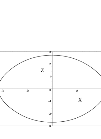
Figure 1: The surface of the rotating polytrope is shown for $\beta=8\times 10^{-2}$ ($X=\xi\sin\theta$ and $Z=\xi\cos\theta$ are Cartesian-like coordinates). The polar and equatorial radii are given by $\xi_{-}\approx 2.7117$ and $\xi_{+}\approx 4.3302$ respectively, in agreement with both James ($\xi_{-}\approx 2.7194$, $\xi_{+}\approx 4.3797$) james and Williams ($\xi_{-}\approx 2.7175$, $\xi_{+}\approx 4.2733$) williams results.

III.2 The effective geometry

The acoustic metric (23) associated with Williams’ solution is given by the line element

$$ds^{2} = \frac{\rho_{0}}{c}[-(c^{2}-v_{0}^{2})dt^{2}-2v_{0}r\sin\theta dtd\phi+dr^{2}+r^{2}(d\theta^{2}+\sin^{2}\theta d\phi^{2})]$$ (38)

$$= \frac{\rho_{0}}{c}[-c^{2}dt^{2}+dr^{2}+r^{2}d\theta^{2}+r^{2}\sin^{2}\theta(\Omega dt-d\phi)^{2}]\,,$$

where $v_{0}=\Omega r\sin\theta$, $c=\sqrt{2K\rho_{0}}$ and the background density $\rho_{0}=\rho_{c}\Theta$. Here the coordinate time-lines have a unit tangent vector ${1}/\sqrt{-g_{tt}}\partial_{t}$ ( with $g_{tt}=-\rho_{0}(c^{2}-v_{0}^{2})/c$) which changes its causality relation when $v_{0}^{2}=c^{2}$, as it happens for instance in the case of Minkowsky flat space-time expressed in uniformly rotating cylindrical coordinates $(t,R,\phi,z)$, i.e.

$$ds^{2}=-(C^{2}-\Omega^{2}R^{2})dt^{2}+2\Omega R^{2}dtd\phi+dR^{2}+R^{2}d\phi^{2}+dz^{2}$$ (39)

at the the so called light cylinder $r=C/\Omega$ where $C$ is the speed of lightLLFIELD . Moreover in relation with metric (38), $\partial_{t}$ is a Killing vector field which is not vorticity-free (i.e. not hyper-surface orthogonal). The form (38) of the metric suggests the introduction of the following coordinate transformation

$$\phi^{\prime}=\phi-\Omega t\ ,\quad t^{\prime}=t$$ (40)

such that we obtain

$$ds^{2}=\frac{\rho_{0}}{c}\left(-c^{2}dt^{\prime 2}+dr^{2}+r^{2}d\theta^{2}+r^{2}\sin^{2}\theta d\phi^{\prime 2}\right)\ .$$ (41)

The new temporal lines have now a unit tangent vector ${1}/\sqrt{-g_{t^{\prime}t^{\prime}}}\partial_{t^{\prime}}$ (with $g_{t^{\prime}t^{\prime}}=-\rho_{0}c$) which never changes its causality condition inside the star. $\partial_{t^{\prime}}$ is still a Killing vector field whose norm is $-\rho_{0}c$ and it is vorticity-free, hence hyper-surface orthogonal . Such a result is not unexpected because it is exactly what happens for the Minkowskian metric (39) in the case of the two Killing vectors $\partial_{t}$ (not vorticity free) and $\partial_{t}+\Omega\partial_{\phi}$ (vorticity free). Since there exists everywhere a time-like Killing vector field which is hyper-surface orthogonal, the space-time of uniformly rotating polytropic stars under exam is staticExact ; Wald . Clearly such a simplification due to the uniform rotation should not apply for differentially rotating configurations which are expected instead to lead to stationary space-times.

Using now the dimensionless variables $\xi$ and $\eta$ defined by

$$r=\alpha\xi\,,\qquad\eta=\sqrt{4\pi G\rho_{c}}\,t^{\prime}\ ,$$ (42)

with $\alpha=\sqrt{K/(2\pi G)}$, leads to the following final form of the metric

$$ds^{2} = \sqrt{\Theta}\left[-\Theta d\eta^{2}+d\xi^{2}+\xi^{2}(d\theta^{2}+\sin^{2}\theta d\phi^{2})\right]\ ,$$ (43)

where we have replaced $\phi^{\prime}$ by $\phi$ for convenience and the ignorable constant multiplicative factor $2\pi G\sqrt{K\rho_{c}/2}$ has been dropped, since it can be re-absorbed in the definitions of $\eta$ and $\xi$ by a simple rescaling of such variables. The metric determinant is given by $g=-\Theta^{3}\xi^{4}\sin^{2}\theta$, so that $\sqrt{-g}=\Theta^{3/2}\xi^{2}\sin\theta$, which implies that the volume element vanishes approaching both the center of the configuration where $\Theta=1$ and the boundary where $\Theta=0$, and it is well behaved otherwise.

It is useful to evaluate the Kretschmann invariantExact ${\cal K}=R_{\alpha\beta\gamma\delta}R^{\alpha\beta\gamma\delta}$. It diverges at the boundary, whereas gets a constant value at the center (see Fig. 2). In fact, its behavior for $\xi\to 0$ is given by

$${\cal K}\simeq\frac{2b_{2}^{2}}{15\pi}+\frac{13}{12}(1-\beta)^{2}+O(\xi^{2})\,.$$ (44)

Other relevant curvature invariants are listed in Appendix A.

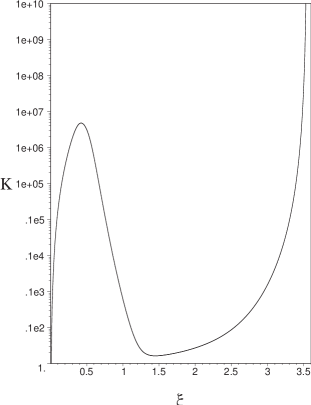
Figure 2: The behavior of the Kretschmann invariant ${\cal K}$ is shown as a function of $\xi$ for $\beta=8\times 10^{-2}$ and fixed $\theta=\pi/3$. The boundary is located at $\xi\approx 3.54$. ${\cal K}$ diverges there, whereas gets a constant value at the center.

It is worth noting that curvature invariants give useful informations about the presence of possible curvature pathologies, whereas the analysis of the metric tensor and its determinant (the latter being a tensor density) do not contain intrinsic information about the spacetime, but only coordinate-dependent informations.

The equations governing geodesic motion are given by

$$\dot{\eta} = \frac{E}{\Theta^{3/2}}\,,$$ (45a)

$$\dot{\phi} = \frac{L}{\sqrt{\Theta}\xi^{2}\sin^{2}\theta}\,,$$ (45b)

$${\dot{\xi}}^{2} = -\xi^{2}{\dot{\theta}}^{2}-\frac{\sigma^{2}}{\sqrt{\Theta}}-\frac{L^{2}}{\xi^{2}\Theta\sin^{2}\theta}+\frac{E^{2}}{\Theta^{2}}\,,$$ (45c)

$$\ddot{\theta} = -\frac{1}{2}\left(\frac{4}{\xi}+\frac{\partial_{\xi}\Theta}{\Theta}\right){\dot{\xi}}{\dot{\theta}}-\frac{1}{2}\left[{\dot{\theta}}^{2}+\frac{\sigma^{2}}{2\xi^{2}\sqrt{\Theta}}+\frac{E^{2}}{\xi^{2}\Theta^{2}}\right]\frac{\partial_{\theta}\Theta}{\Theta}+\frac{\cos\theta}{\sin^{3}\theta}\frac{L^{2}}{\xi^{4}\Theta}\,,$$ (45d)

where Killing symmetries and the normalization condition have been used. Here $E$ and $L$ are constants of motion (representing energy and angular momentum), $\sigma^{2}=1,0,-1$ for timelike, null and spatial geodesics respectively and a dot denotes differentiation with respect to the affine parameter.

Let us consider first the motion on the equatorial plane $\theta=\pi/2$. If $\theta=\pi/2$ and $\dot{\theta}=0$ initially, Eq. (45d) ensures that the motion will be confined on the equatorial plane, since $\partial_{\theta}\Theta$ vanishes at $\theta=\pi/2$, so that $\ddot{\theta}=0$ too. The geodesic equations thus reduce to

$$\dot{\eta} = \frac{E}{\Theta^{3/2}}\,,\qquad\dot{\phi}=\frac{L}{\sqrt{\Theta}\xi^{2}}\,,\qquad{\dot{\xi}}^{2}=-\frac{\sigma^{2}}{\sqrt{\Theta}}-\frac{L^{2}}{\xi^{2}\Theta}+\frac{E^{2}}{\Theta^{2}}\,,$$ (46)

where the function $\Theta$ is meant to be evaluated at $\theta=\pi/2$. The $\xi$–motion turns out to be governed by the effective potential $V_{\xi}$, implicitly defined by

$$-\frac{\sigma^{2}}{\sqrt{\Theta}}-\frac{L^{2}}{\xi^{2}\Theta}+\frac{V_{\xi}^{2}}{\Theta^{2}}=0\,.$$ (47)

In fact, for $E=V_{\xi}$ the right hand side of the last equation of Eq. (46) vanishes.

Similarly, one can introduce the effective potential governing the $\theta$-motion, i.e. with $\xi=\,$const:

$$-\frac{\sigma^{2}}{\sqrt{\Theta}}-\frac{L^{2}}{\xi^{2}\Theta\sin^{2}\theta}+\frac{V_{\theta}^{2}}{\Theta^{2}}=0\,,$$ (48)

as from Eq. (45c) where we set $\dot{\xi}=0$.

III.3 Perturbations

The set of equations governing fluctuations about the unperturbed reference flow are given by Eq. (II.3). This is a system of coupled PDEs which cannot be solved analytically. Even a direct numerical integration in the time domain is a hard task as discussed later.

The problem can be simplified by noting that the contribution of $\vec{\xi}_{1}$ to the first order velocity field is generally a small correction with respect to $\nabla\psi_{1}$, as discussed in Ref. ROTA . The system (II.3) thus becomes

$$\nabla^{\mu}\nabla_{\mu}\psi_{1} = -\frac{c}{\rho_{0}}\left(\frac{D^{(0)}}{dt}\right)\left(\frac{\Phi_{1}}{c^{2}}\right)\,,$$

$$\left[\nabla^{2}+k_{J}^{2}\right]\Phi_{1} = -k_{J}^{2}\frac{D^{(0)}}{dt}\psi_{1}\,,$$ (49)

with $\vec{\xi}_{1}$ neglected. It is worth to stress that the quantity $\vec{\xi}_{1}$ represents the correction to potential flow induced by angular momentum conservation, with a partial hybridization of the sound with other modes. At low frequencies (see Ref. ROTA ) the contribution by $\vec{\xi}_{1}$ ceases to be negligible and the sound waves hybridize with the many other modes available for a fluid whose vorticity can have comparable frequency. In our analysis, however, we shall be far from this scenario.

By neglecting also the gravitational back-reaction, linear perturbations of the velocity potential satisfy the Klein-Gordon equation for a massless scalar field $\nabla^{\mu}\nabla_{\mu}\psi_{1}=0$ on the background metric (43), i.e.

$$\left[-\frac{\partial^{2}}{\partial\eta^{2}}+\Theta\nabla^{2}+\partial_{\xi}\Theta\frac{\partial}{\partial\xi}+\frac{\partial_{\theta}\Theta}{\xi^{2}}\frac{\partial}{\partial\theta}\right]\psi_{1}=0\ ,$$ (50)

where $\nabla^{2}$ is the ordinary Laplacian in spherical coordinates. Unfortunately this equation is not completely separable, so it should be studied numerically.

However, one expects that the analog light cone (or sound cone) structure of our problem resulting from the numerical integration of the wave equation (50) is related to null geodesics (i.e. Eqs. (45a)–(45d) with $\sigma=0$) in a standard way, in the sense that these are the high frequency limit of $\psi_{1}$. Fig. 3 (a) shows the behavior of the effective potential $V_{\xi}$ for radial motion of null rays on the equatorial plane $\theta=\pi/2$ and fixed values of the rotation parameter $\beta$. We see that the center of the configuration is approached only by high energy rays. Fig. (b) shows instead the typical path of a sound ray starting from the equatorial plane at a given distance from the center with fixed energy and angular momentum. The behavior of the effective potential $V_{\theta}$ for polar motion of null rays is shown in Figs. 4 (a) and 5 (a) for fixed values of the radial parameter $\xi<\xi_{-}$ and $\xi>\xi_{-}$, respectively. In the first case the motion is confined between two values of the polar angle for fixed energy, whereas in the latter case the ray can reach the boundary of the configuration. The corresponding spherical orbits of a ray starting from the equatorial plane with fixed energy and angular momentum are shown in Figs. 4 (b)–(d) and 5 (b)–(d), respectively.

The analog light cone structure is obtained by setting $ds^{2}=0$ in Eq. (43). For instance, the equation governing the motion of accelerated null rays moving radially on the equatorial plane turns out to be given by

$$\frac{d\xi}{d\eta}=\pm\sqrt{\Theta}\ ,$$ (51)

where $\Theta$ is evaluated at $\theta=\pi/2$. The sound cone structure arising from the numerical integration of Eq. (51) is shown in Fig. 6. Note that the boundary is reached at a finite time as in the spherical case bcfprd .

$\begin{array}[]{cc}\includegraphics[scale={0.5}]{fig3a.eps}&\includegraphics[scale={0.5}]{fig3b.eps}\\[11.38092pt] \quad\mbox{(a)}&\quad\mbox{(b)}\end{array}$

Figure 3: The effective potential $V_{\xi}$ for radial motion of null rays is shown in Fig. (a) for $\theta=\pi/2$ and fixed values of $\beta=8\times 10^{-2}$ and $L=1$. Fig. (b) shows the path of a sound ray starting from the equatorial plane with energy $E=1$ and angular momentum $L=1$ at $X=3$.

$\begin{array}[]{cc}\includegraphics[scale={0.45}]{fig4a.eps}&\quad\includegraphics[scale={0.5}]{fig4b.eps}\\[11.38092pt] \quad\mbox{(a)}&\quad\mbox{(b)}\\[17.07182pt] \includegraphics[scale={0.45}]{fig4c.eps}&\quad\includegraphics[scale={0.45}]{fig4d.eps}\\[11.38092pt] \quad\mbox{(c)}&\quad\mbox{(d)}\end{array}$

Figure 4: The effective potential $V_{\theta}$ for polar motion of null rays is shown in Fig. (a) for $\xi=2.5<\xi_{-}$ and fixed values of $\beta=8\times 10^{-2}$ and $L=1$ ($X=\xi\sin\theta\cos\phi$, $Y=\xi\sin\theta\sin\phi$ and $Z=\xi\cos\theta$ are Cartesian-like coordinates). The boundary surface has been cut in half for a better view of the interior. The corresponding spherical orbit of a ray starting from the equatorial plane with energy $E=1$ is shown in Fig. (b). The projected path on both planes $X-Y$ and $X-Z$ is shown in Figs. (c) and (d), respectively.

$\begin{array}[]{cc}\includegraphics[scale={0.45}]{fig5a.eps}&\quad\includegraphics[scale={0.5}]{fig5b.eps}\\[11.38092pt] \quad\mbox{(a)}&\quad\mbox{(b)}\\[17.07182pt] \includegraphics[scale={0.45}]{fig5c.eps}&\quad\includegraphics[scale={0.45}]{fig5d.eps}\\[11.38092pt] \quad\mbox{(c)}&\quad\mbox{(d)}\end{array}$

Figure 5: The effective potential $V_{\theta}$ for polar motion of null rays is shown in Fig. (a) for $\xi=3>\xi_{-}$ and fixed values of $\beta=8\times 10^{-2}$ and $L=3$. The corresponding spherical orbit of a ray starting from the equatorial plane with energy $E=1$ is shown in Fig. (b). The projected path on both planes $X-Y$ and $X-Z$ is shown in Figs. (c) and (d), respectively. The numerical integration stops when the boundary of the configuration is reached.

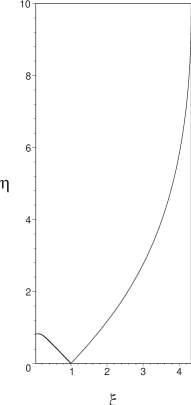
Figure 6: Analog light cone structure for radially accelerated sound rays starting at the point $\xi=1$ for $\eta=0$ from the equatorial plane $\theta=\pi/2$ for $\beta=8\times 10^{-2}$. The boundary $\xi\approx 4.33$ is reached at a finite time.

IV Concluding remarks

In this paper we have derived the field equations for general acoustic perturbations of a perfect rotating and self-gravitating compressible gaseous/fluid mass through an extended analog model based on Clebsch potentials, here generalized to account for gravitational backreaction.

We have then examined in detail the case of the uniformly rotating $n=1$ polytropic configuration as an analytical background mainly focusing on the geometric properties of the associated acoustic metric.

The surface of the star, as in the spherical case bcfprd , corresponds to a zero density condition, so that the sound speed vanishes, while the curvature of the spacetime diverges (the geometry breaks down manifesting a curvature singularity). A simple explanation of the curvature divergence, even in presence of rotation, is that acoustics require a medium on which waves travel. The fluid is the source of the induced metric tensor, but on the surface of the star there is no medium, so there cannot be sound too: geometric analogies fail here.

The presence of rotation leads in general to a stationary problem with an ergosphere where the fluid velocity exceeds the local speed of sound. Stationarity, however, must be associated with a differential rotation of the fluid. In the simplest uniformly rotating case considered here the metric is indeed static, leading to a relatively simple dynamics. On the other hand the case of differential rotation should provide more complicated situations in which such a simplification could not be achievable anymore.

Our study could be useful to better understand the non relativistic theory of stellar and galactic structures via methods typical of General Relativity. In particular, a problem which still remains to be studied is how, for uniformly or differentially rotating polytropes, our perturbative geometrized formulation can describe instabilities leading to bifurcations similar to those already discussed in the literature using different mathematical approaches (see e.g. Ref. Tholine ). In this context in particular it would be important to see if in case of outer fluid layers rotating with supersonic velocities, there could be a superradiant scattering of sound waves, already evidenced in acoustic black holes (see Ref. CHR1 and references therein) as it happens for astrophysical systems as black holes. This possible analysis requires however an important technical clarification. In black hole physics in fact the perturbation analysis in search of instabilities can be performed by analytical techniques due to the complete separability of the perturbation equation in radial and angular variables in the frequency domain, leading to a Schroedinger-like problem Chandra . Unfortunately, in the present context such a simplification does not occur due to the non variables separability of density and speed of sound so the whole analysis then can only be performed numerically including the ordinary differential equations of geodesics discussed in this article. The perturbative equations in particular are partial differential equations leading to an involved study which would require in the time domain the implementation of specific numerical codes in $``3+1"$ or $``2+1"$ (using axisymmetry of the background) dimensions written using modern numerical relativity tools, and therefore is left to future works on the lines of Refs. CHR1 ; CHR2 .

Appendix A Newman-Penrose quantities

The following Newman-Penrose frame (we follow Ref. Frolov for conventions here) allows one to study in detail the curvature structure of the acoustic metric (43):

$$l=\frac{1}{\sqrt{2}}(e_{\hat{\eta}}+e_{\hat{\xi}})\,,\qquad n=\frac{1}{\sqrt{2}}(e_{\hat{\eta}}-e_{\hat{\xi}})\,,\qquad m=\frac{1}{\sqrt{2}}(e_{\hat{\theta}}+ie_{\hat{\phi}})\ ,$$ (52)

where

$$e_{\hat{\eta}}=\frac{1}{\sqrt{-g_{\eta\eta}}}\partial_{\eta}\ ,\quad e_{\hat{\xi}}=\frac{1}{\sqrt{g_{\xi\xi}}}\partial_{\xi}\ ,\quad e_{\hat{\theta}}=\frac{1}{\sqrt{g_{\theta\theta}}}\partial_{\theta}\ ,\quad e_{\hat{\phi}}=\frac{1}{\sqrt{g_{\phi\phi}}}\partial_{\phi}\ .$$ (53)

The nonvanishing spin coefficients are

$$\kappa = \frac{1}{4\sqrt{2}}\frac{\Theta_{\theta}}{\Theta^{5/4}\xi}=\frac{\tau}{2}=\nu=\frac{\pi}{2}\ ,$$

$$\epsilon = -\frac{3}{8\sqrt{2}}\frac{\Theta_{\xi}}{\Theta^{5/4}}=\gamma\ ,$$

$$\alpha = \frac{\kappa}{2}+\frac{1}{2\sqrt{2}}\frac{\cot\theta}{\Theta^{1/4}\xi}=-\beta\ ,$$

$$\rho = -\frac{2}{3}\epsilon+\frac{1}{\sqrt{2}}\frac{1}{\Theta^{1/4}\xi}=-\mu\ .$$ (54)

The Weyl scalar in this frame are

$$\psi_{0} = \psi_{4}=\frac{1}{8\Theta^{3/2}\xi^{2}}\left[\Theta_{\theta\theta}-\Theta_{\theta}\left(\frac{\Theta_{\theta}}{2\Theta}+\cot\theta\right)\right]\ ,$$

$$\psi_{1} = -\psi_{3}=-\frac{1}{8\Theta^{3/2}\xi}\left[\Theta_{\xi\theta}-\Theta_{\theta}\left(\frac{\Theta_{\xi}}{2\Theta}+\frac{1}{\xi}\right)\right]\ ,$$

$$\psi_{2} = \frac{1}{6\Theta^{3/2}}\left[\Theta_{\xi\xi}-\frac{\Theta_{\theta\theta}}{2\xi^{2}}-\Theta_{\xi}\left(\frac{\Theta_{\xi}}{2\Theta}+\frac{1}{\xi}\right)+\frac{\Theta_{\theta}}{2\xi^{2}}\left(\frac{\Theta_{\theta}}{2\Theta}-\cot\theta\right)\right]\ .$$ (55)

Other nonvanishing NP quantities are the curvature scalar

$$R=\frac{5}{2\Theta^{3/2}}\left[\Theta_{\xi\xi}+\frac{\Theta_{\theta\theta}}{\xi^{2}}-2\Theta_{\xi}\left(\frac{7}{40}\frac{\Theta_{\xi}}{\Theta}-\frac{1}{\xi}\right)-\frac{\Theta_{\theta}}{\xi^{2}}\left(\frac{7}{20}\frac{\Theta_{\theta}}{\Theta}-\cot\theta\right)\right]\,,$$ (56)

and the Ricci coefficients

$$\Phi_{00} = \Phi_{22}=\frac{1}{8\Theta^{3/2}}\left[\Theta_{\xi\xi}-\frac{\Theta_{\theta\theta}}{\xi^{2}}-2\Theta_{\xi}\left(\frac{7}{8}\frac{\Theta_{\xi}}{\Theta}+\frac{1}{\xi}\right)-\frac{\Theta_{\theta}}{\xi^{2}}\cot\theta\right]\ ,$$

$$\Phi_{11} = -\Phi_{00}-\frac{R}{40}-\frac{21}{160\Theta^{5/2}}\left(\Theta_{\xi}^{2}+\frac{\Theta_{\theta}^{2}}{\xi^{2}}\right)\ ,$$

$$\Phi_{01} = -\Phi_{12}=\frac{1}{4\Theta^{3/2}\xi}\left[\Theta_{\xi\theta}-\Theta_{\theta}\left(\frac{7}{8}\frac{\Theta_{\xi}}{\Theta}+\frac{1}{\xi}\right)\right]\ ,$$

$$\Phi_{02} = \frac{1}{4\Theta^{3/2}\xi^{2}}\left[\Theta_{\theta\theta}-\Theta_{\theta}\left(\frac{7}{8}\frac{\Theta_{\theta}}{\Theta}+\cot\theta\right)\right]\ .$$ (57)

The behavior of the independent Weyl scalars as well as the Ricci scalar is shown as a function of $\xi$ for fixed $\theta$ in Figs. 7 and 8, respectively. All quantites diverge at the boundary, whereas get a constant value at the center. In fact, for $\xi\to 0$ we have

$$\psi_{0} \simeq \frac{1}{20}\frac{b_{2}}{\sqrt{2\pi}}\sin^{2}\theta+O(\xi^{2})\,,$$

$$\psi_{1} \simeq \frac{1}{20}\frac{b_{2}}{\sqrt{2\pi}}\sin\theta\cos\theta+O(\xi^{2})\,,$$

$$\psi_{2} \simeq \frac{1}{60}\frac{b_{2}}{\sqrt{2\pi}}(3\cos^{2}\theta-1)+O(\xi^{2})\,,$$

$$R \simeq \frac{5}{2}(1-\beta)+O(\xi^{2})\,.$$ (58)

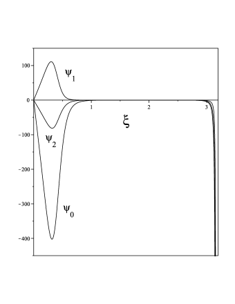
Figure 7: The independent Weyl scalars $\psi_{0}$, $\psi_{1}$ and $\psi_{2}$ are plotted as functions of $\xi$ for $\beta=8\times 10^{-2}$ and fixed $\theta=\pi/4$. The boundary is located at $\xi\approx 3.17$. They all diverge there, whereas get a constant value at the center.

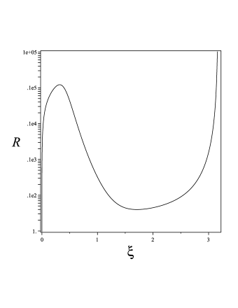
Figure 8: The behavior of the Ricci scalar $R$ is shown as a function of $\xi$ for $\beta=8\times 10^{-2}$ and fixed $\theta=\pi/4$. It diverges at the boundary ($\xi\approx 3.17$), whereas gets a constant value at the center.

References

- (1) W. G. Unruh, Phys. Rev. D 51, 2827 (1995).
- (2) M. Visser, Class. Quantum Grav. 15, 1767 (1998).
- (3) C. Barceló, S. Liberati, and M. Visser, Analogue Gravity, Living Rev. Relativity, 8, (2005), 12. URL (cited on 02/22/2010): http://www.livingreviews.org/lrr-2005-12
- (4) M. Novello, M. Visser, and G. E. Volovik (Editors), Artificial Black Holes (World Scientific, Singapore, 2002).
- (5) W. Unruh and R. Schutzhold, Quantum Analogues: From Phase Transitions to Black Holes and Cosmology, Lect. Notes Phys. 718 (Springer, Berlin, 2007).
- (6) D. Bini, C. Cherubini, and S. Filippi, Phys. Rev. D 78, 064024 (2008).
- (7) J. L. Tassoul, Theory of Rotating Stars (Princeton University Press, Princeton, NJ, 1978).
- (8) J. Binney and S. Tremaine, Galactic Dynamics (Princeton University Press, Princeton, NJ, 1987).
- (9) J. Ostriker, Astrophys. Jour. 140, 1506 (1964).
- (10) P. S. Williams, Astrophys. Space Sci. 143, 349 (1988).
- (11) G. P. Horedt, Polytropes: Applications in Astrophysics and Related Fields (Springer, New York, 2004).
- (12) L. D. Landau and E. M. Lifshitz, The Classical Theory of Fields 4th Edition,(Butterwoth-Heineman, Oxford, (1975).
- (13) H. Stegani, D. Kramer, M. MacCallum, C. Hoenselaers, E. Herlt, Exact Solution to Einstein’s Field Equations 2nd Edition, Cambridge University Press, (2003).
- (14) R.Wald, General Relativity, University of Chicago Press, (1984).
- (15) S. E. P. Bergliaffa, K. Hibberd, M. Stone, and M. Visser, Physica D 191, 121 (2004).
- (16) H. Lamb, Hydrodynamics (Dover Publications, New York, 1993).
- (17) T. Kambe, Elementary Fluid Mechanics (World Scientific, Singapore, 2007).
- (18) W. Greiner, Relativistic Quantum Mechanics: Wave Equations (Springer, New York, 2000).
- (19) W. Greiner, J. Reinhardt, and D. A. Bromley, Field Quantization (Springer, New York, 2008).
- (20) L. D. Landau and E. M. Lifshitz, Fluid Mechanics 2nd Edition,(Butterwoth-Heineman, Oxford, (2004).
- (21) Taniguchi K., Nakamura T., Phys Rev Lett. Jan 84 581-5 (2000).
- (22) F. Weber, Pulsars as Astrophysical Laboratories for Nuclear and Particle Physics (Taylor and Francis, Bristol, 1999).
- (23) J. M. Lattimer and M. Prakash, Astrophys. Jour. 550, 426 (2001).
- (24) N. Stergioulas, ”Rotating Stars in Relativity”, Living Rev. Relativity 6, 3, (2003).
- (25) S. Chandrasekhar, An Introduction to the Study of Stellar Structure (Dover Publications, New York, 1958).
- (26) R. James, Astrophys. Jour. 140, 552 (1964).
- (27) J.M. Imamura, J.L Friedman and R.H. Durisen, APJ 290, p.474-478 (1985).
- (28) S. Chandrasekhar, Ellipsoidal Figures of Equilibrium (Dover Publications, New York, 1969).
- (29) C. Cherubini F. Federici, S. Succi, and M.P. Tosi, Phys. Rev. D 72, 084016 (2005).
- (30) H. A. Williams and J. E. Tohline, Astrophys. Jour. 315, 594 (1987).
- (31) F. Federici, C. Cherubini, S. Succi, and M. P. Tosi, Phys. Rev. A 73, 033604 (2006).
- (32) V. Frolov and I. Novikov, Black Hole Physics: Basic Concepts and New Developments (Springer, New York, 1998).