Sound waves and modulational instabilities on continuous wave solutions in spinor Bose-Einstein condensates

Abstract

We analyze sound waves (phonons, Bogoliubov excitations) propagating on continuous wave (cw) solutions of repulsive $F=1$ spinor Bose-Einstein condensates (BECs), such as ²³Na (which is anti-ferromagnetic or polar) and ⁸⁷Rb (which is ferromagnetic). Zeeman splitting by a uniform magnetic field is included. All cw solutions to ferromagnetic BECs with vanishing $M_{F}=0$ particle density and non-zero components in both $M_{F}=\pm 1$ fields are subject to modulational instability (MI). Modulational instability increases with increasing particle density. Modulational instability also increases with differences in the components’ wave numbers; this effect is larger at lower densities but becomes insignificant at higher particle densities. Continuous wave solutions to anti-ferromagnetic (polar) BECs with vanishing $M_{F}=0$ particle density and non-zero components in both $M_{F}=\pm 1$ fields do not suffer MI if the wave numbers of the components are the same. If there is a wave number difference, MI initially increases with increasing particle density, then peaks before dropping to zero beyond a given particle density. The cw solutions with particles in both $M_{F}=\pm 1$ components and non-vanishing $M_{F}=0$ components do not have MI if the wave numbers of the components are the same, but do exhibit MI when the wave numbers are different. Direct numerical simulations of a cw with weak white noise confirm that weak noise grows fastest at wave numbers with the largest MI, and show some of the results beyond small amplitude perturbations. Phonon dispersion curves are computed numerically; we find analytic solutions for the phonon dispersion in a variety of limiting cases.

I Introduction

Bose-Einstein condensates (BECs) Bose.1924 ; Einstein.1924 ; Einstein.1925 ; Anderson.1995 ; Davis.1995 hold the promise of opening many new vistas in physics, e.g., macroscopic systems that exhibit quantum effects, higher resolution measurements of time, inertia, and other quantities, and a medium with which to carry out quantum computing and to simulate quantum systems Feynman.1986 ; CiracZoller.2012 ; Lahav.2010 ; Gorshkov.2010 ; Lewenstein.2012 . Many interesting phenomena in BECs either occur against simpler backgrounds or are prepared from initially simpler states, which are often plane waves or approximations thereof. For example, vortices Saito.2007 ; Lamacraft.2007 ; UhlmannSchutzholdFischer.2007 ; KawaguchiUeda.2012 and dark solitons Burger.1999 ; Denschlag.2000 ; Li.2005 are typically imbedded on plane waves, and a spin texture Sadler.2006 may be composed of, in part, many regions that are approximately plane waves. When the dynamics of plane waves are understood better, the structures that sit on them may be understood better. It is useful to know—especially if those simpler states are not quite as simple as had been thought—when they can and cannot exhibit more complex dynamics, and what those dynamics are.

Bose-Einstein condensates can be composed of particles with non-zero total angular momentum ($F>0$). For example, there is $H$ Fried.1998 , ⁷Li Bradley.1997 , ²³Na Davis.1995 ; Simkin.1999 , ⁴¹K Modugno.2001 , ⁵²Cr Griesmaier.2005 , ⁸⁴Sr Stellmer.2009 , ⁸⁵Rb Cornish.2000 , ⁸⁷Rb Anderson.1995 , ¹³³Cs Weber.2003 , ¹⁶⁴Dy Lu.2011 , and ¹⁷⁰Yb Fukuhara.2007 . An optical (as opposed to magnetic) trap can hold all the spin components ($M_{F}=-F,-F+1,\ldots,F-1,F$) Barrett.2001 ; Chang.2004 ; Beaufils.2008 ; Leslie.2009 . In this case the BEC field is a spinor with $2F+1$ $M_{F}$ components, and can exhibit phenomena that do not occur in scalar fields. First and foremost, there is magnetism. More complicated phenomena in spinor BECs that do not occur in a scalar BEC are some forms of MI Robins.2001 ; Konotop.2002 ; Li.2005 ; Zhang.MI.2005 ; Kunimi.2014 , oscillatory coherent spin mixing Zhang.spin_mixing.2005 ; MurPetit.2009 ; TasgalBand.2013 , formation of spin textures, i.e., patterns of spatial variation of the magnetization Sadler.2006 , and certain forms of vortices with magnetization Sadler.2006 ; Saito.2007 ; Lamacraft.2007 ; UhlmannSchutzholdFischer.2007 , including fractional vortices and non-Abelian vortices KawaguchiUeda.2012 .

Here we examine sound waves (phonons, acoustic waves, Bogoliubov excitations) that propagate on top of continuous wave (cw) solutions of $F=1$ spinor BECs Mewes.1996 ; Andrews.1997 ; Andrews.1998 ; Steinhauer.2002 ; Ozeri.2005 ; Bogolubov.1947 . When the frequencies of the sound waves have (do not have) imaginary parts, they grow exponentially (do not grow), which implies that the background is unstable (stable). Sound waves with imaginary parts are most often called MI or Benjamin-Feir instabilities BespalovTalanov.1966 ; BenjaminFeir.1967 ; Agrawal.2001 ; there are instances where it has been called self-pulsing instability Agrawal.2001 or dynamical instability KawaguchiUeda.2012 . Section II introduces the equations for the dynamics of an $F=1$ spinor BEC, the general form of the cw solutions, and sets out the formalism for describing small amplitude sound waves. Section III computes the phonon band diagrams, i.e., the way the frequencies (chemical potentials) of the sound waves depend on wave number. Special attention is paid to complex-valued frequencies, since this, MI, causes the sound waves to grow exponentially. Section IV presents direct numerical simulations, which confirm the analytic results for small amplitude phonons, and investigates the evolution of large amplitude (highly nonlinear) noise. Section V summarizes.

II Quantitative model for spinor BECs with magnetic fields

The Hamiltonian density for an $F=1$ spinor BEC with linear and quadratic Zeeman splittings induced by a magnetic field ${\bf B}=B\,\hat{\bf z}$ (and without spin-dipolar coupling) is OhmiMachida.1998 ; Ho.1998 ; StamperKurnUeda.2013

$$\mathcal{H} = \frac{\hbar^{2}}{2m}\mathbf{\nabla}\Phi_{a}^{\dagger}\cdot\mathbf{\nabla}\Phi_{a}+\frac{c_{0}}{2}\Phi_{a}^{\dagger}\Phi_{b}^{\dagger}\Phi_{b}\Phi_{a}+\frac{c_{2}}{2}\Phi_{a}^{\dagger}\Phi_{a^{\prime}}^{\dagger}\mathbf{F}_{ab}\cdot\mathbf{F}_{a^{\prime}b^{\prime}}\Phi_{b^{\prime}}\Phi_{b}-pB\Phi_{a}^{\dagger}F^{z}_{ab}\Phi_{b}+qB^{2}\Phi_{a}^{\dagger}(F^{z}_{ab})^{2}\Phi_{b}\,.$$ (1)

Here $\Phi=(\phi_{1},\phi_{0},\phi_{-1})^{\mathrm{t}}$ is a vector composed of the amplitudes of spin $M_{F}=1$, $M_{F}=0$, and $M_{F}=-1$. $m$ is the mass of the particles, $c_{0}$ and $c_{2}$ are the coefficients of the spin-independent and spin-dependent parts of the mean field, ${\bf F}$ is the total atomic angular momentum vector and each component is a 3$\times$3 spin-1 matrix; $B$ is the magnitude of the (uniform) external magnetic field, which is taken to be in the $z$-direction, and $p$ and $q$ are linear and quadratic Zeeman coefficients Saito.2007 ; Lamacraft.2007 ; Zhang.spin_mixing.2005 . The results here actually apply to any strength Zeeman effect, and are not limited to magnetic fields small enough for the dependence of the particle energies as a function of $B$ to be described by the first two terms of a Taylor expansion. To generalize, substitute relative particle energies as a function of spin state $[E_{m=+1}(B)-E_{m=-1}(B)]/2$ for $pB$ and $[E_{m=+1}(B)+E_{m=-1}(B)-2E_{m=0}(B)]/2$ for $qB^{2}$. Within the limitations of this paper, $[E_{m=+1}(B)+E_{m=0}(B)+E_{m=-1}(B)]/3$ is a global energy shift, and may be neglected.

If the BEC is in a quasi-one-dimensional optical trap with population only in a single transverse bound state, the governing equations are

$$i\hbar\frac{\partial}{\partial t}\phi_{1} = -\frac{\hbar^{2}}{2m}\frac{\partial^{2}}{\partial z^{2}}\phi_{1}+c_{0}\left(|\phi_{1}|^{2}+|\phi_{0}|^{2}+|\phi_{-1}|^{2}\right)\phi_{1}+c_{2}\left[\left(|\phi_{1}|^{2}+|\phi_{0}|^{2}-|\phi_{-1}|^{2}\right)\phi_{1}+\phi_{0}^{2}\phi_{-1}^{*}\right]$$ (2a)

$$\;\;\;\;\;\;\;\;\;\;\;\;\;\;\;\;\;\;\;\;+(-pB+qB^{2})\phi_{1}\,,$$

$$i\hbar\frac{\partial}{\partial t}\phi_{0} = -\frac{\hbar^{2}}{2m}\frac{\partial^{2}}{\partial z^{2}}\phi_{0}+c_{0}\left(|\phi_{1}|^{2}+|\phi_{0}|^{2}+|\phi_{-1}|^{2}\right)\phi_{0}+c_{2}\left[\left(|\phi_{1}|^{2}+|\phi_{-1}|^{2}\right)\phi_{0}+2\phi_{1}\phi_{0}^{*}\phi_{-1}\right]\,,$$ (2b)

$$i\hbar\frac{\partial}{\partial t}\phi_{-1} = -\frac{\hbar^{2}}{2m}\frac{\partial^{2}}{\partial z^{2}}\phi_{-1}+c_{0}\left(|\phi_{1}|^{2}+|\phi_{0}|^{2}+|\phi_{-1}|^{2}\right)\phi_{-1}+c_{2}\left[\left(-|\phi_{1}|^{2}+|\phi_{0}|^{2}+|\phi_{-1}|^{2}\right)\phi_{-1}+\phi_{0}^{2}\phi_{1}^{*}\right]$$ (2c)

$$\;\;\;\;\;\;\;\;\;\;\;\;\;\;\;\;\;\;\;\;\;\;+(pB+qB^{2})\phi_{-1}\,.$$

Time and space are $t$ and $z$, $c_{0}$ is a coefficient of self-phase modulation, and $c_{2}$ is a coefficient of both self-phase modulation and parametric nonlinearity (and is spin-dependent). Materials with negative $c_{2}$ are ferromagnetic, and materials with positive $c_{2}$ are anti-ferromagnetic, or polar. The nonlinear coefficients are functions of the particle mass $m$ and the s-wave scattering lengths $a_{0}$, $a_{2}$ for the $F=0$ and $F=2$ channels, $g_{0}=(4\pi\hbar^{2}/m)a_{0}$, $g_{2}=(4\pi\hbar^{2}/m)a_{2}$, with the nonlinear coefficients in the governing equations above $c_{0}=(g_{0}+2g_{2})/3$, $c_{2}=-(g_{0}-g_{2})/3$. The values of the nonlinear coefficients are modified when the BEC is in a trap Olshanii.1998 ; Bergeman.2003 . The scattering lengths of ⁸⁷Rb are $a_{0}=101.8\,a_{B}$ and $a_{2}=a_{0}-1.45\,a_{B}$, where $a_{B}$ is the Bohr radius Chang.2005 ; KlausenBohnGreene.2001 ; KempenKokkelmansHeinzenVerhaar.2002 , and the scattering lengths of ²³Na have been measured to be $a_{0}=50.0\,a_{B}$, $a_{2}=a_{0}+5.0\,a_{B}$. The ratios $c_{2}/c_{0}$ are $-0.0048$ for ⁸⁷Rb and $0.031$ for ²³Na. Equations (2) are integrable when $c_{2}=0$ (in which case the system is a set of generalized Manakov equations Nakkeeran.1998 ; Manakov.1973 ) or $c_{2}=c_{0}$ IedaMiyakawaWadati.2004 ; WadatiTsuchida.2006 ; IedaWadati.2007 .

Equations (2) can be written in dimensionless form by applying a change of variables

$$t^{\prime} = t/t_{d},$$ (3a)

$$z^{\prime} = z/z_{d}=z/\sqrt{\hbar t_{d}/m},$$ (3b)

$$\phi_{j}^{\prime} = \phi_{j}/\phi_{d}=\phi_{j}/\sqrt{\hbar/(c_{0}t_{d})}.$$ (3c)

The dimensionless equations have $\hbar=1$, $m=1$, $c_{0}=1$, and $c_{2}|_{\mathrm{dimensionless}}=c_{2}/c_{0}$. The dimensionless frequencies and wave numbers go as the dimensional variables times $t_{d}$ and $z_{d}=\sqrt{\hbar t_{d}/m}$, respectively. $t_{d}$ is a free variable, and may be chosen such that the dimensionless time, space, or amplitudes are convenient magnitudes. We will use dimensionless variables in the figures in order to emphasize generality, but retain the dimensions in the body of the text to more closely connect the equations to the physical parameters.

A important observable is the magnetization vector $\mathbf{m}=(m_{x},m_{y},m_{z})$. For a spin $F=1$ BEC, this is the spin-vector density, which is equal to the expectation value of the spin-vector $\mathbf{F}=(F_{x},F_{y},F_{z})$, where

$$F_{x}=\frac{1}{\sqrt{2}}\left(\begin{matrix}0&1&0\\ 1&0&1\\ 0&1&0\end{matrix}\right),\;F_{y}=\frac{1}{\sqrt{2}}\left(\begin{matrix}0&-i&0\\ i&0&-i\\ 0&i&0\end{matrix}\right),\;F_{z}=\left(\begin{matrix}1&0&0\\ 0&0&0\\ 0&0&-1\end{matrix}\right),$$ (4)

multiplied by the maximum magnetic moment of the particles that constitute the BEC. For the dimensionless variables, we take the maximum magnetic moment to be unity. That gives the dimensionless magnetization vector

$$\mathbf{m}=\left(\begin{matrix}m_{x}\\ m_{y}\\ m_{z}\end{matrix}\right)=\left(\begin{matrix}\mathrm{Re}[\sqrt{2}(\phi_{1}+\phi_{-1})^{*}\phi_{0}]\\ \mathrm{Im}[\sqrt{2}(\phi_{1}-\phi_{-1})^{*}\phi_{0}]\\ |\phi_{1}|^{2}-|\phi_{-1}|^{2}\end{matrix}\right).$$ (5)

If any two of the three spin fields are zero, then the remaining field is governed by a simple nonlinear Schrödinger (NLS) equation, called the Gross–Pitaevskii equation, which is completely integrable ZakharovShabat.1971 ; ZakharovShabat.1973 . If the $M_{F}=0$ component spin field vanishes ($\phi_{0}=0$), then the spin $M_{F}=\pm 1$ fields ($\phi_{1}$, $\phi_{-1}$) are governed by a pair of coupled nonlinear Schrödinger (CNLS) equations,

$$i\hbar\frac{\partial}{\partial t}\phi_{1} = -\frac{\hbar^{2}}{2m}\frac{\partial^{2}}{\partial z^{2}}\phi_{1}+\left[(c_{0}+c_{2})|\phi_{1}|^{2}+(c_{0}-c_{2})|\phi_{-1}|^{2}\right]\phi_{1}\,,$$ (6a)

$$i\hbar\frac{\partial}{\partial t}\phi_{-1} = -\frac{\hbar^{2}}{2m}\frac{\partial^{2}}{\partial z^{2}}\phi_{-1}+\left[(c_{0}-c_{2})|\phi_{1}|^{2}+(c_{0}+c_{2})|\phi_{-1}|^{2}\right]\phi_{-1}\,,$$ (6b)

which have been intensely studied (see, e.g., Ref. Yang.2010 ). They describe, among other physical systems, light in optical fibers Agrawal.2001 . In optics, one convention is to describe the ratio of the coefficients of cross- to self-phase modulation as $B=(c_{0}-c_{2})/(c_{0}+c_{2})$. Linear polarization in optics is described by $B=2/3$, which corresponds to a ratio $c_{2}/c_{0}=1/5$; circular polarization in optics has $B=2$, which corresponds to $c_{2}/c_{0}=-1/3$. Because of the positive and negative signs of the corresponding $c_{2}/c_{0}$, the dynamics of linearly polarized light resembles the dynamics of repulsive ferromagnetic BECs, and circularly polarized light resembles anti-ferromagnetic (polar) BECs, provided the BECs do not contain any particles with spin $m=0$. The CNLS equations for light in a fiber often contain group-velocity birefringence terms. These terms may be eliminated by a transformation that changes variables: shifts the frequencies and wave numbers of the component fields [see, e.g., Eq. (7.2.29) in Agrawal.2001 ]. Changing the group-velocity birefringence (e.g., setting it to zero) corresponds to shifting the wave numbers of the spin $m=+1,-1$ up and down, respectively.

II.1 Continuous wave solutions

We begin by considering the solutions of the dynamical equations with the simplest shape, a flat constant field, or cw. The most general cw ansatz is

$$\phi_{1} = A_{1}\exp[i(\theta_{1}+k_{1}z-\omega_{1}t)]\,,$$ (7a)

$$\phi_{0} = A_{0}\exp[i(\theta_{0}+k_{0}z-\omega_{0}t)]\,,$$ (7b)

$$\phi_{-1} = A_{-1}\exp[i(\theta_{-1}+k_{-1}z-\omega_{-1}t)]\,,$$ (7c)

where the parameters are real-valued and, without loss of generality, $A_{j}$ are positive definite. Spin components with different wave numbers have, in general, different velocities. In this model, the domain is infinite. In an experiment (or in numerical simulations), a BEC with different wave numbers in the different spin components would need to be long enough to avoid edge effects, or one could replenish the fields at the boundaries, or arrange the fields in a ring (confined by a toroidal potential) Gupta.2005 ; Olson.2007 ; Lesanovsky.2007 ; Henderson.2009 ; Ryu.2007 . In a ring, the wave numbers would be quantized, but otherwise all the results would hold. Modulation instability of spinor BECs in a ring geometry has been studied theoretically in Ref. Kunimi.2014 .

Let us substitute the cw trial function (7) into the dynamical equations (2). If $c_{2}=0$, there are cw solutions for every value of the amplitude ($A_{j}$), wave number ($k_{j}$), and phase ($\theta_{j}$). The frequencies of the fields are

$$\hbar\omega_{j}=\frac{\hbar^{2}k_{j}^{2}}{2m}+c_{0}(A_{1}^{2}+A_{0}^{2}+A_{-1}^{2})\,.$$ (8)

If $c_{2}\neq 0$, then the parametric term requires a relation between the phases of the three fields,

$$k_{0} = \frac{1}{2}(k_{1}+k_{-1})\,,$$ (9a)

$$\omega_{0} = \frac{1}{2}(\omega_{1}+\omega_{-1})\,,$$ (9b)

$$\theta_{0} = \frac{1}{2}(\theta_{1}+\theta_{-1}+n\pi)\,,$$ (9c)

where $n$ is an integer. The frequencies of the spin components $M_{F}=1,0,-1$ are

$$\hbar\omega_{1} = \frac{\hbar^{2}k_{1}^{2}}{2m}+c_{0}\left(A_{1}^{2}+A_{0}^{2}+A_{-1}^{2}\right)+c_{2}\left[A_{1}^{2}+A_{0}^{2}-A_{-1}^{2}+(-1)^{n}A_{0}^{2}A_{-1}/A_{1}\right]+(-pB+qB^{2})A_{1}\,,$$ (10a)

$$\hbar\omega_{0} = \frac{\hbar^{2}k_{0}^{2}}{2m}+c_{0}\left(A_{1}^{2}+A_{0}^{2}+A_{-1}^{2}\right)+c_{2}\left[A_{1}^{2}+A_{-1}^{2}+2(-1)^{n}A_{1}A_{-1}\right]\,,$$ (10b)

$$\hbar\omega_{-1} = \frac{\hbar^{2}k_{-1}^{2}}{2m}+c_{0}\left(A_{1}^{2}+A_{0}^{2}+A_{-1}^{2}\right)+c_{2}\left[-A_{1}^{2}+A_{0}^{2}+A_{-1}^{2}+(-1)^{n}A_{0}^{2}A_{1}/A_{-1}\right]+(pB+qB^{2})A_{-1}\,.$$ (10c)

For consistency of the frequency $\omega_{0}$ of the $M_{F}=0$ field, [Eqs. (10) and (9b)], the magnitude $A_{0}$ of the $M_{F}=0$ field must be

$$A_{0}^{2}=2(-1)^{n}A_{1}A_{-1}\left(1-\frac{(\hbar^{2}/2m)[(k_{1}-k_{-1})/2]^{2}+qB^{2}}{c_{2}[A_{1}+(-1)^{n}A_{-1}]^{2}}\right).$$ (11)

The left hand side of Eq. (11) is real and non-negative. If $c_{2}<0$ (ferromagnetic), for the right hand side to be positive, the cw solutions must have even $n$ (for conciseness, we write $n=0$ to denote even $n$ and $n=1$ for odd $n$). If $c_{2}>0$ (anti-ferromagnetic), then over certain ranges of the cw spin-components $M_{F}=\pm 1$, there are only $n=0$ solutions, both $n=0$ and $n=1$ solutions, or only $n=1$ solutions; there is always at least one cw solutions with non-vanishing $M_{F}=0$ field, with the exception of $M_{F}=\pm 1$ particle densities exactly equal to each other and below the threshold at which $n=0$ cws exist, $A_{1}^{2}=A_{-1}^{2}<(4c_{2})^{-1}[\hbar^{2}(k_{1}-k_{-1})^{2}/8m+qB^{2}]$. For the $n=0$ and $n=1$ type cw solutions, there is a particle density $A_{\mathrm{ref}}$ which roughly separates the regimes in which linear components of the energy are more important from regimes in which nonlinear polarization-dependent components of the energy are more important. Taking the internal (in the reference frame in which the spin $m=0$ field has wave number zero) kinetic energy plus the quadratic Zeeman energy, i.e., all the linear terms, to be $E_{\mathrm{lin}}=\{\hbar^{2}[(k_{1}-k_{-1})/2]^{2}/(2m)+qB^{2}\}|A_{\mathrm{ref}}|^{2}$ and the energy scale of the nonlinear polarization-dependent terms as $E_{\mathrm{NL}}=c_{2}|A_{\mathrm{ref}}|^{4}$, the particle density at which the absolute values of these linear and nonlinear energies are equal is $A_{\mathrm{ref}}^{2}=|\{\hbar^{2}[(k_{1}-k_{-1})/2]^{2}/(2m)+qB^{2}\}/c_{2}|$. This reference particle density is a rough marker for the blurred boundary between the two regimes. See Ref. TasgalBand.2013 for a more detailed elucidation of the consequences of Eq. (11). The dimensionless magnetization components of this cw are

$$m_{x} = \mathrm{Re}\{(i)^{n}\sqrt{2}A_{0}[A_{1}\exp(i\phi_{\Delta}/2)+A_{-1}\exp(-i\phi_{\Delta}/2)]\},$$ (12a)

$$m_{y} = \mathrm{Im}\{(i)^{n}\sqrt{2}A_{0}[A_{1}\exp(i\phi_{\Delta}/2)-A_{-1}\exp(-i\phi_{\Delta}/2)]\},$$ (12b)

$$m_{z} = |A_{1}|^{2}-|A_{-1}|^{2},$$ (12c)

where the phase difference between the $+1$ and $-1$ components is $\phi_{\Delta}\equiv\phi_{1}-\phi_{-1}+(k_{1}-k_{-1})z-(\omega_{1}-\omega_{-1})t$. The magnetization is flat in the “natural” orientation direction (z) of the cw and sinusoidal in space and time in the transverse directions.

II.2 Sound waves and modulational instabilities

Sound waves in BECs have been studied experimentally in, e.g., Refs. Mewes.1996 ; Andrews.1997 ; Andrews.1998 ; Steinhauer.2002 ; Ozeri.2005 . In the context of mean field theory, sound waves (or by other names, acoustic waves, phonons, or Bogoliubov excitations) and also MI (where sound waves have complex-valued frequencies) may be represented by small perturbations to a cw solution Bogolubov.1947 ; BespalovTalanov.1966 ; BenjaminFeir.1967 ; Menyuk.1987 ; Agrawal.1987 ; Agrawal.2001 ; Berman.2002 ; Robins.2001 ; HuangLiSzeftel.2004 ; Li.2005 ; Zhang.MI.2005 ; Kunimi.2014 ,

$$\phi_{j}=[A_{j}+a_{j}(z,t)]\exp[i(\theta_{j}+k_{j}z-\omega_{j}t)]\,,$$ (13)

where $j=1,0,-1$. It is convenient to define the frequencies and wave numbers of the phonons with respect to the cw solution on which it propagates, rather than $\phi_{j}=A_{j}\exp[i(\theta_{j}+k_{j}z-\omega_{j}t)]+a_{j}(z,t)$.

III Phonon dispersion band diagrams

The dynamics of sound waves on top of the cw solutions are obtained by substituting the ansatz (13) into the governing equations (2). If the sound waves are weak, one may linearize in the perturbations $a_{j}$. The perturbations then have superposition, and the general solution is a sum of sound waves. This allows a spectral approach. Look for solutions one frequency and wave number at a time, i.e., eigenvalues and eigenvectors,

$$a_{j}(z,t)=p_{j}\cos(kz-\omega t)+iq_{j}\sin(kz-\omega t).$$ (14)

The phonons are here represented in terms of sines and cosines, but they could equally well be in terms of exponentials. The former tends to be use more often in looking for MI (frequencies with complex values) Agrawal.2001 , while the latter is more typical when considering stable sound waves (Bogoliubov excitations) or more quantum mechanical problems.

There are six equations in $p_{j}$ and $q_{j}$, each of which are complex-valued,

$$0=Mv=\left\{[-\hbar\omega+\frac{\hbar^{2}}{2m}(k_{1}+k_{-1})k]\mathbf{I}+\mathbf{P}+\mathbf{Q}+\mathbf{R}\right\}v\,,$$ (15)

where $v=(p_{1},q_{1},p_{0},q_{0},p_{-1},q_{-1})^{t}$ and

$$\mathbf{P}=\frac{\hbar^{2}k}{2m}\left(\begin{array}[]{cccccc}\Delta k&k&0&0&0&0\\ k&\Delta k&0&0&0&0\\ 0&0&0&k&0&0\\ 0&0&k&0&0&0\\ 0&0&0&0&-\Delta k&k\\ 0&0&0&0&k&-\Delta k\end{array}\right)$$ (16a)

$$\mathbf{Q}=2\left(\begin{array}[]{cccccc}0&0&0&0&0&0\\ (c_{0}+c_{2})A_{1}^{2}&0&(c_{0}+c_{2})A_{1}A_{0}&0&(c_{0}-c_{2})A_{1}A_{-1}&0\\ 0&0&0&0&0&0\\ (c_{0}+c_{2})A_{1}A_{0}&0&c_{0}A_{0}^{2}&0&(c_{0}+c_{2})A_{0}A_{-1}&0\\ 0&0&0&0&0&0\\ (c_{0}-c_{2})A_{1}A_{-1}&0&(c_{0}+c_{2})A_{0}A_{-1}&0&(c_{0}+c_{2})A_{-1}^{2}&0\end{array}\right),$$ (16b)

$$\mathbf{R}=(-1)^{n}c_{2}\left(\begin{array}[]{cccccc}0&-A_{0}^{2}A_{-1}/A_{1}&0&2A_{0}A_{-1}&0&-A_{0}^{2}\\ -A_{0}^{2}A_{-1}/A_{1}&0&2A_{0}A_{-1}&0&A_{0}^{2}&0\\ 0&2A_{0}A_{-1}&0&-4A_{1}A_{-1}&0&2A_{1}A_{0}\\ 2A_{0}A_{-1}&0&0&0&2A_{1}A_{0}&0\\ 0&-A_{0}^{2}&0&2A_{1}A_{0}&0&-A_{0}^{2}A_{1}/A_{-1}\\ A_{0}^{2}&0&2A_{1}A_{0}&0&-A_{0}^{2}A_{1}/A_{-1}&0\end{array}\right).$$ (16c)

Note that the frequency (chemical potential) $\omega$ of the perturbations (relative to the cw on which it sits) and the average wave number $k_{0}=(k_{1}+k_{-1})/2$ appear only on the diagonal. Off-diagonal terms depend on the parameters of the cw, $A_{1}$, $A_{-1}$, $\Delta k\equiv k_{1}-k_{-1}$, and $n$; note that $A_{0}$ is a function of the other cw parameters [Eq. (11)]. $c_{2}/c_{0}$ cannot be simplified or reduced to more trivial terms. The linear and quadratic Zeeman effects do not appear explicitly. The quadratic Zeeman terms appear implicitly in the magnitude of $A_{0}$. The quadratic Zeeman splitting will affect the perturbations of the cw solutions with non-zero $M_{F}=0$ fields, but will not affect the cases without an $M_{F}=0$ field.

Equations (15)–(16) constitute an eigenvalue–eigenvector problem, with solutions being six eigenvalues $\omega_{j}=\omega_{j}(k)$, with eigenvectors $(p_{j,i}(k),q_{j,i}(k))$, $j=1,\ldots,6$. Some insights into the phonon dispersion curves may be obtained by expanding the characteristic polynomial $|M|$ from Eqs. (15)–(16), in energy $\hbar\omega$ and wave number $k$. We may express the sixth-order polynomial equation for the eigenvalues (frequencies or energies of the sound waves or Bogoliubov excitations), leaving the dependence on the background cw implicit in the coefficients,

$$0 = (\hbar\omega)^{6}+(C_{k^{0}\omega^{4}}^{\mathrm{cw}(n=0,1)}+C_{k^{2}\omega^{4}}^{\mathrm{cw}(n=0,1)}k^{2}+C_{k^{4}\omega^{4}}^{\mathrm{cw}(n=0,1)}k^{4})(\hbar\omega)^{4}+(C_{k^{1}\omega^{3}}^{\mathrm{cw}(n=0,1)}k+C_{k^{3}\omega^{3}}^{\mathrm{cw}(n=0,1)}k^{3})(\hbar\omega)^{3}$$ (17)

$$+ (C_{k^{2}\omega^{2}}^{\mathrm{cw}(n=0,1)}k^{2}+C_{k^{4}\omega^{2}}^{\mathrm{cw}(n=0,1)}k^{4}+C_{k^{6}\omega^{2}}^{\mathrm{cw}(n=0,1)}k^{6}+C_{k^{8}\omega^{2}}^{\mathrm{cw}(n=0,1)}k^{8})(\hbar\omega)^{2}$$

$$+ (C_{k^{3}\omega}^{\mathrm{cw}(n=0,1)}k^{3}+C_{k^{5}\omega}^{\mathrm{cw}(n=0,1)}k^{5}+C_{k^{7}\omega}^{\mathrm{cw}(n=0,1)}k^{7})(\hbar\omega)$$

$$+ C_{k^{4}\omega^{0}}^{\mathrm{cw}(n=0,1)}k^{4}+C_{k^{6}\omega^{0}}^{\mathrm{cw}(n=0,1)}k^{6}+C_{k^{8}\omega^{0}}^{\mathrm{cw}(n=0,1)}k^{8}+C_{k^{10}\omega^{0}}^{\mathrm{cw}(n=0,1)}k^{10}+C_{k^{12}\omega^{0}}^{\mathrm{cw}(n=0,1)}k^{12}.$$

There are six dispersion curves, corresponding, at any given waveumber, to six mutually orthogonal phonon perturbations. The coefficients $C_{k^{i}\omega^{j}}^{\mathrm{cw}(n=0,1)}=(i!j!)^{-1}\partial_{k}^{i}\partial_{\omega}^{j}|M|$ are too lengthy to be included explicitly in full in the body of the text. From the band diagrams, $\omega=\omega_{j}(k)$, come the energies of the phonons, $\hbar\mathrm{Re}[\omega_{j}(k)]$, the MI $\mathrm{Im}[\omega_{j}(k)]$, phase velocities $v_{p}=\mathrm{Re}[\omega_{j}(k)]/k$, group velocities $v_{g}=(d/dk)\{\mathrm{Re}[\omega_{j}(k)]\}$, phonon group velocity dispersion values $(d^{2}/dk^{2})\{\mathrm{Re}[\omega_{j}]\}=(d/dk)v_{g}$, and higher-order dispersion $(d^{n}/dk^{2})\{\mathrm{Re}[\omega_{j}]\}$, where $n>2$. Solving involves finding the roots of a sixth-order polynomial. Numerical solutions may be readily obtained. The general case is not analytically soluble. There are analytic solutions in some limiting and special cases.

In the case with zero particle density of spin $M_{F}=0$, the equation for the phonons in spin states $M_{F}=\pm 1$ is the same as for the CNLS equation,

$$0=(\hbar\omega)^{4}+(C_{k^{2}\omega^{2}}^{\mathrm{CNLS}}k^{2}+C_{k^{4}\omega^{2}}^{\mathrm{CNLS}}k^{4})(\hbar\omega)^{2}+C_{k^{3}\omega}^{\mathrm{CNLS}}k^{3}(\hbar\omega)+C_{k^{4}\omega^{0}}^{\mathrm{CNLS}}k^{4}+C_{k^{6}\omega^{0}}^{\mathrm{CNLS}}k^{6}+C_{k^{8}\omega^{0}}^{\mathrm{CNLS}}k^{8},$$ (18)

which are well-known from optics. This is in principle soluble, though the solutions for a quartic polynomial is long even with simple coefficients, and for spinor BECs the coefficients are not very short.

III.1 Special cases with full analytic phonon bands

There are a few cases for which the whole dispersion band function is available analytically. If two of the three spin fields are zero, the frequency of the cw is $\hbar\omega_{j}=\frac{\hbar k_{j}^{2}}{2m}+2cA_{j}^{2}$, where $c=c_{0}+c_{2}$ for spin $M_{F}=j=\pm 1$, and $c=c_{0}$ for spin $M_{F}=j=0$. Sound waves on top of this cw have frequency

$$\hbar\omega=\frac{\hbar^{2}k_{j}}{m}k\pm\sqrt{\frac{\hbar^{2}k^{2}}{2m}\left(\frac{\hbar^{2}k^{2}}{2m}+2cA_{j}^{2}\right)}.$$ (19)

Equation (19) is the well-known Bogoliubov dispersion relation Bogolubov.1947 . When the nonlinearity is repulsive or zero ($c\geq 0$), the frequencies are real-valued, and all the cw solutions are stable. When the nonlinearity is attractive ($c<0$), there are sound waves with complex-valued frequencies, i.e., MI, for wave numbers $\hbar^{2}k^{2}/(2m)<-2cA_{j}^{2}$. The largest MI is at wave numbers $k=\pm\sqrt{-2mc}A_{j}/\hbar$, and the growth rate is $\mathrm{Im}(\omega)=-cA_{j}^{2}/\hbar$ BespalovTalanov.1966 .

For perturbations on top of cws with nil $M_{F}=0$ fields, the eigenvalues (energies, frequencies, chemical potentials) are roots of fourth-order polynomials, which can be solved in terms of roots. In the limiting case in which the wave numbers are the same ($k_{1}=k_{-1}$), the phonon frequency as a function of wave number, i.e., the band diagram, is

$$\hbar\omega=qB^{2}\pm\left(\frac{\hbar^{2}k^{2}}{2m}\right)^{1/2}\left(\frac{\hbar^{2}k^{2}}{2m}+(c_{0}+c_{2})(A_{1}^{2}+A_{-1}^{2})\pm\left\{\left[(c_{0}+c_{2})(A_{1}^{2}+A_{-1}^{2})\right]^{2}-16c_{0}c_{2}A_{1}^{2}A_{-1}^{2}\right\}^{1/2}\right)^{1/2}.$$ (20)

Two of the four branches of the phonon solutions in Eq. (20) contains frequencies with complex parts, i.e., modulational instabilities, when the BEC is ferromagnetic, $c_{2}<0$, such as is the case for ⁸⁷Rb; the frequencies are real-valued for anti-ferromagnetic BECs, $c_{2}\geq 0$. There are analytic solutions for phonons in the general CNLS case, where the cw contains non-zero wave number differences. However, we found the general formulas for sound waves in the $M_{F}=\pm 1$ fields to be long and complex to the point that computational efficiency but little understanding could be gained from the exact solutions.

For the ferromagnetic CNLS–type phonons, the largest MI (imaginary component of the frequency) and the wave numbers (up to a sign, and offset with respect to the average of the wave numbers) at which they occur, $(k_{1}-k_{-1})/2$, are

$$\omega_{\mathrm{MI}}^{\mathrm{CNLS}}(k_{1}=k_{-1}) \equiv \frac{1}{2\hbar}\left[\sqrt{[(c_{0}+c_{2})(A_{1}^{2}+A_{-1}^{2})]^{2}-16c_{0}c_{2}A_{1}^{2}A_{-1}^{2}}-(c_{0}+c_{2})(A_{1}^{2}+A_{-1}^{2})\right],$$ (21a)

$$k_{\mathrm{MI}}^{\mathrm{CNLS}}(k_{1}=k_{-1}) \equiv \sqrt{\frac{2m}{\hbar}\omega_{\mathrm{MI}}^{\mathrm{CNLS}}(k_{1}=k_{-1})},$$ (21b)

which is similar to Bogoliubov dispersion Bogolubov.1947 and MI in the NLS equation BespalovTalanov.1966 , though with different parameters. The MI range is $|k|<2k_{\mathrm{MI}}^{\mathrm{CNLS}}(k_{1}=k_{-1})$. Since there is no MI above a certain wavelength, the cw should fail to manifest MI if the domain is periodic with length less than or equal to $\pi/k_{\mathrm{MI}}^{\mathrm{CNLS}}(k_{1}=k_{-1})$.

For the CNLS case, the small-amplitude (linearized) $M_{F}=0$ fields decouple from the $M_{F}=\pm 1$ phonons, and have simple analytic solutions,

$$\hbar\omega=\pm\left\{\left[\frac{\hbar^{2}k^{2}}{2m}+c_{2}(A_{1}^{2}+A_{-1}^{2})-qB^{2}-\frac{\hbar^{2}}{2m}\left(\frac{k_{1}-k_{-1}}{2}\right)^{2}\right]^{2}-4c_{2}^{2}A_{1}^{2}A_{-1}^{2}\right\}^{1/2}\,.$$ (22)

The cw will be modulationally stable in the $M_{F}=0$ field if

$$E_{\mathrm{MI}}^{\mathrm{crit}}\equiv c_{2}[A_{1}-\mathrm{sign}(c_{2})A_{-1}]^{2}-qB^{2}-\frac{\hbar^{2}}{2m}\left(\frac{k_{1}-k_{-1}}{2}\right)^{2}\geq 0,$$ (23)

and subject to MI if $E_{\mathrm{MI}}^{\mathrm{crit}}<0$. In the unstable case, the maximum MI values occur at wave number (recall that the system is being analyzed in a reference frame in which $k_{1}+k_{-1}=0$) $k=0$ if

$$c_{2}(A_{1}^{2}+A_{-1}^{2})-qB^{2}-(\hbar^{2}/2m)[(k_{1}-k_{-1})/2]^{2}\geq 0,$$ (24)

yielding peak MI

$$\max[\mathrm{Im}(\omega)]=\hbar^{-1}\sqrt{4c_{2}^{2}A_{1}^{2}A_{-1}^{2}-[c_{2}(A_{1}^{2}+A_{-1}^{2})-qB^{2}-\hbar^{2}(k_{1}-k_{-1})^{2}/(8m)]^{2}}\,;$$ (25)

otherwise, the maximum MI occurs at phonons that are combinations of

$$k=\pm\sqrt{(k_{1}-k_{-1})^{2}/4-(2m/\hbar^{2})[c_{2}(A_{1}^{2}+A_{-1}^{2})-qB^{2}]},$$ (26a)

yielding peak MI

$$\max[\mathrm{Im}(\omega)]=2|c_{2}|A_{1}A_{-1}/\hbar.$$ (26b)

There are analytic solutions for the band diagram of sound waves on $n=0$ type cws in the limiting case in which the wave numbers are all the same ($k_{1}=k_{0}=k_{-1}$) and the quadratic Zeeman splitting is zero,

$$\omega = \pm\frac{\hbar k^{2}}{2m},$$ (27a)

$$\omega = \pm\frac{1}{\hbar}\left[\frac{(\hbar k)^{2}}{2m}-2c_{2}(A_{1}+A_{-1})^{2}\right],$$ (27b)

$$\omega = \pm\frac{1}{\hbar}\sqrt{\frac{(\hbar k)^{2}}{2m}\left[\frac{(\hbar k)^{2}}{2m}+2(c_{0}+c_{2})(A_{1}+A_{-1})^{2}\right]}.$$ (27c)

It follows from Eqs. (27) that the cws have MI if and only if $c_{0}+c_{2}<0$. This is not the case for either ²³Na or ⁸⁷Rb, so for these the $n=0$ cws are stable when the wave numbers are all the same and quadratic Zeeman splitting is absent. Thus, ironically, in ferromagnetic BECs, the ($n=0$)–type cw solutions are modulationally stable and the CNLS–type solutions have MI, even though the former cws have higher energy than the latter. We failed to find analytic formulas for the phonons when there was quadratic Zeeman splitting or non-zero differences in the wave numbers of the spin components $M_{F}$.

III.2 Small and large wave number (k) limiting cases

III.2.1 Continuous wave background solutions of types n=0,1

In the large wave number limit, the equation for the band diagram for sound waves on top of the cw($n=0,1$) solutions approaches (in dimensionless units)

$$0 = (\omega^{2}/k^{4})^{3}+C_{k^{4}\omega^{4}}^{\mathrm{cw}(n=0,1)}(\omega^{2}/k^{4})^{4}+C_{k^{8}\omega^{2}}^{\mathrm{cw}(n=0,1)}(\omega^{2}/k^{4})+C_{k^{12}\omega^{0}}^{\mathrm{cw}(n=0,1)}$$ (28)

$$= (\omega^{2}/k^{4})^{3}-(3/4)(\omega^{2}/k^{4})^{4}+(3/16)(\omega^{2}/k^{4})-1/64$$

$$= (\omega^{2}/k^{4}-1/4)^{3},$$

or, with the dimensions left in, $\omega=\pm\hbar k^{2}/(2m)$. At large wave numbers, the kinetic terms dominate over the nonlinearities, and the dispersion approaches a quadratic dependence on the wave number (i.e., constant dispersion), the same as it would be in the absence of nonlinearities. In the limit of small wave numbers ($k\approx 0$), the dispersion curves can be obtained by substituting a Taylor expansion,

$$\omega(k)=\omega_{0}+\omega_{1}k+\frac{1}{2}\omega_{2}k^{2}+\ldots\,,$$ (29)

into the equation (17) for the complete dispersion curve.

Two of the phonon dispersion curves at low momentum (small $|k|$) have Taylor coefficients

$$\omega_{0} = \pm\sqrt{-C_{k^{0}\omega^{4}}^{\mathrm{cw}(n=0,1)}},$$ (30a)

$$\omega_{1} = C_{k^{1}\omega^{3}}^{\mathrm{cw}(n=0,1)}/(2C_{k^{0}\omega^{4}}^{\mathrm{cw}(n=0,1)}),$$ (30b)

$$\omega_{2} = -\frac{1}{\omega_{0}}\left(C_{k^{2}\omega^{4}}^{\mathrm{cw}(n=0,1)}-\frac{C_{k^{2}\omega^{2}}^{\mathrm{cw}(n=0,1)}}{C_{k^{2}\omega^{4}}^{\mathrm{cw}(n=0,1)}}+\frac{3C_{k^{1}\omega^{3}}^{\mathrm{cw}(n=0,1)}}{4(C_{k^{0}\omega^{4}}^{\mathrm{cw}(n=0,1)})^{2}}\right),$$ (30c)

and four dispersion curves have $\omega_{0}=0$ for the 0th-order in the expansion, and the linear terms in the dispersion curves are the roots of the quartic equation in $\omega_{1}$,

$$0=C_{k^{0}\omega^{4}}^{\mathrm{cw}(n=0,1)}\hbar^{4}\omega_{1}^{4}+C_{k^{1}\omega^{3}}^{\mathrm{cw}(n=0,1)}\hbar^{3}\omega_{1}^{3}+C_{k^{2}\omega^{2}}^{\mathrm{cw}(n=0,1)}\hbar^{2}\omega_{1}^{2}+C_{k^{3}\omega}^{\mathrm{cw}(n=0,1)}\hbar\omega_{1}+C_{k^{4}\omega^{0}}^{\mathrm{cw}(n=0,1)}.$$ (31)

Explicit analytic formulas for higher orders in the expansion of the dispersion curves do not seem very useful, so we stop at this order.

III.2.2 cw background solutions with zero particle density for spin m=0

In the large wave number limit, the band diagram of phonons on top of cw solutions without an $M_{F}=0$ component approaches $\omega=\pm\hbar k^{2}/(2m)$. At large wave numbers, the kinetic terms dominate over the nonlinearities, and the dispersion approaches a quadratic dependence on the wave number (i.e., constant dispersion), the same as it would be in the absence of nonlinearities. In the limit of small wave numbers ($k\approx 0$), the dispersion curves can be obtained by substituting a Taylor expansion

$$\omega(k)=\omega_{0}+\omega_{1}k+\frac{1}{2}\omega_{2}k^{2}+....$$ (32)

into the equation (18) for the CNLS dispersion curve. The 0th-order term is nil ($\omega_{0}$). The first-order terms ($\omega_{1}$)—one for each of the four curves—are the solutions of the quartic polynomial

$$0=\hbar^{4}\omega_{1}^{4}+C_{k^{2}\omega^{2}}^{\mathrm{CNLS}}\hbar^{2}\omega_{1}^{2}+C_{k^{3}\omega}^{\mathrm{CNLS}}\hbar\omega_{1}+C_{k^{4}\omega^{0}}^{\mathrm{CNLS}}.$$ (33)

We stop at the linear expansion terms because general explicit analytic formulas for the higher-order terms in the series are not very helpful. One may carry out the expansion numerically for specific cw solutions.

III.3 Band diagram illustrations

To illustrate the range of different behaviors in the sound waves and the MI, we show the real parts of the frequencies [$\mathrm{Re}(\omega)$] and MI [$\mathrm{Im}(\omega)$] versus the wave number of sound waves propagating on a background of each of the allowed cws in a BEC of (i) ²³Na and (ii) ⁸⁷Rb, in which the wave numbers of the different spin components are (a) all identical and (b) when the wave numbers have different values. Each of the examples in Figs. 1-9 takes the dimensionless amplitudes of the $M_{F}=\pm 1$ fields to be $A_{1}=2$ and $A_{-1}=2.5$, and the quadratic Zeeman splitting is zero.

In the CNLS–type solutions, the $M_{F}=0$ particle density is zero; the (dimensionless) Hamiltonians for ⁸⁷Rb are $52.5191$ when the wave vectors are the same (corresponding to Fig. 1), and $53.8004$ when $k_{1}-k_{-1}=1$ (corresponding to Fig. 2); the Hamiltonians for ²³Na are $52.5877$ when the wave vectors are the same (corresponding to Fig. 3), and $53.8689$ when $k_{1}-k_{-1}=1$ (corresponding to Fig. 4). Of the ($n=0$)–type cw solutions, a ⁸⁷Rb BEC has $A_{0}=3.16228$ and $H=204.288$ when the wave vectors are the same (corresponding to Fig. 5), and $A_{0}=4.78308$ and $H=548.323$ when $k_{1}-k_{-1}=1$ (corresponding to Fig. 6); and the ($n=0$)–type cw in a ²³Na BEC has $A_{0}=3.16228$ and $H=52.5877$ when the wave vectors are the same (corresponding to Fig. 7), and $A_{0}=2.68906$ and $H=156.589$ when $k_{1}-k_{-1}=1$ (corresponding to Fig. 8). For the ($n=1$)–type cw solution for ²³Na with $k_{1}-k_{-1}=1$ (corresponding to Fig. 9), $A_{0}=14.6385$ and $H=25234.6$.

A sense of the effects of non-zero wave number difference can be gained by comparing Fig. 1 with Fig. 2, Fig. 3 with Fig. 4, Fig. 5 with Fig. 6, and Fig. 7 with Fig. 8. wave number differences in the spin components increase the modulational instability, whether the BECs are ferromagnetic or anti-ferromagnetic, with or without a nontrivial $M_{F}=0$ field. Note that the displayed phonon dispersion curve for a CNLS–type cw in a ²³Na BEC with non-zero difference in the wave numbers (Fig. 4) has zero MI, but similar cws but with smaller particle densities are subject to MI. This is consistent with the well-known fact that (in the language of optical fibers) the cw with components of the same wave number in a pair of CNLS equations without birefringence is stable when the ratio of cross- to self-phase modulation $B=(c_{0}-c_{2})/(c_{0}+c_{2})$ is less than zero (similar to an anti-ferromagnetic BEC), and modulationally unstable when the ratio is greater than zero (similar to a ferromagnetic BEC) Menyuk.1987 ; Agrawal.1987 ; Agrawal.2001 . This also confirms the known result that—recall that group-velocity birefringence terms in CNLS equations can be eliminated by a change in variables in which the frequencies and wave numbers of the cw components are shifted [see, e.g., Eq. (7.2.29) in Agrawal.2001 ]—group-velocity birefringence (which maps to a difference in the wave numbers of the cw components here) adds to the MI. Modulational instability in the CNLS limit with wave number differences has been, for BECs, referred to as the “countersuperflow instability.” Law.2001 ; Tsitoura.2013 . A sense of the difference between ferromagnetic and anti-ferromagnetic BEC can be obtained by comparing Fig. 1 with Fig. 3, Fig. 2 with Fig. 4, Fig. 5 with Fig. 7, and Fig. 6 with Fig. 8. Bose-Einstein condensates of ⁸⁷Rb (ferromagnetic) are more subject to MI than ²³Na (anti-ferromagnetic) for CNLS–type cws and ($n=0$)–type cws with non-zero wave number difference. Continuous waves of type $n=0$ with all spin components at the same wave number are stable against MI for both ⁸⁷Rb and ²³Na. One of the differences between ferromagnetic and anti-ferromagnetic BECs is that only the anti-ferromagnetic ones allow ($n=1$)–type cws, such as with the band diagram in Fig. 9. These cws have MI, but it is weak compared to MI on the other comparable cw solutions. A sense of the differences between the different types of cw solutions (different values of the amplitudes of the spin $M_{F}=0$ component for given $M_{F}=\pm 1$ fields) may be obtained by comparing Fig. 1 with Fig. 5, Fig. 2 with Fig. 6, Fig. 3 with Fig. 7, and Figs. 4, 8, and 9. In ⁸⁷Rb, the $n=0$ cws are more stable against MI than the CNLS–type cws. In ²³Na, there is no MI in either type of cw when the wave numbers are all the same; when there is a wave number difference, the $n=1$ cws have the weakest (but not vanishing) MI, the CNLS cws have stronger MI, and the $n=0$ cws have the greatest MI.

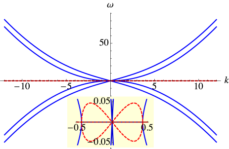
Figure 1: (Color online) Band diagram (frequency as a function of wave vector) for phonons propagating on top of a CNLS–type cw solution (vanishing $M_{F}=0$ field) of a ⁸⁷Rb BEC where the $M_{F}=1$ and $M_{F}=-1$ spin components have the same wave vectors, and amplitudes $2$ and $2.5$. The energies (chemical potentials) come from the real parts of the frequencies ($E=\hbar\mathrm{Re}[\omega]$), which are shown as solid lines; and the MI comes from the imaginary parts of the frequencies, which are dotted lines. All quantities in the figure are dimensionless; see Eqs. (3).

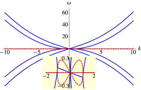
Figure 2: (Color online) Band diagram (frequency as a function of wave vector) for phonons propagating on top of a CNLS–type cw solution (vanishing $M_{F}=0$ field) of a ⁸⁷Rb BEC where the $M_{F}=1$ and $M_{F}=-1$ components have wave vectors that differ by $k_{1}-k_{-1}=1$, and amplitudes $2$ and $2.5$. The energies (chemical potentials) come from the real parts of the frequencies ($E=\hbar\mathrm{Re}[\omega]$), which are shown as solid lines; and the MI comes from the imaginary parts of the frequencies, which are dotted lines. All quantities in the figure are dimensionless; see Eqs. (3).

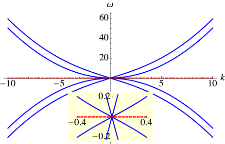
Figure 3: (Color online) Band diagram (frequency as a function of wave vector) for phonons propagating on top of a CNLS–type cw solution (vanishing $M_{F}=0$ field) of a ²³Na BEC where the $M_{F}=1$ and $M_{F}=-1$ spin components have the same wave vectors, and amplitudes $2$ and $2.5$. The energies (chemical potentials) come from the real parts of the frequencies ($E=\hbar\mathrm{Re}[\omega]$), which are shown as solid lines; and the MI comes from the imaginary parts of the frequencies, which are dotted lines. In this case, the frequencies are real-valued, so there is no MI. All quantities in the figure are dimensionless; see Eqs. (3).

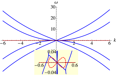
Figure 4: (Color online) Band diagram (frequency as a function of wave vector) for phonons propagating on top of a CNLS–type cw solution (vanishing $M_{F}=0$ field) of a ²³Na BEC where the $M_{F}=1$ and $M_{F}=-1$ components have wave vectors that differ by $k_{1}-k_{-1}=1$, and amplitudes $2$ and $2.5$. The energies (chemical potentials) come from the real parts of the frequencies ($E=\hbar\mathrm{Re}[\omega]$), which are shown as solid lines; and the MI comes from the imaginary parts of the frequencies, which are dotted lines. All quantities in the figure are dimensionless; see Eqs. (3).

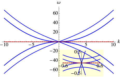
Figure 5: (Color online) Band diagram (frequency as a function of wave vector) for phonons propagating on top of an ($n=0$)–type cw solution of a ⁸⁷Rb BEC where the $M_{F}=1$ and $M_{F}=-1$ spin components have the same wave vectors and amplitudes $2$ and $2.5$. The energies (chemical potentials) come from the real parts of the frequencies ($E=\hbar\mathrm{Re}[\omega]$), which are shown as solid lines. The imaginary parts of the frequencies, shown as dotted lines, are zero, so there is no MI.

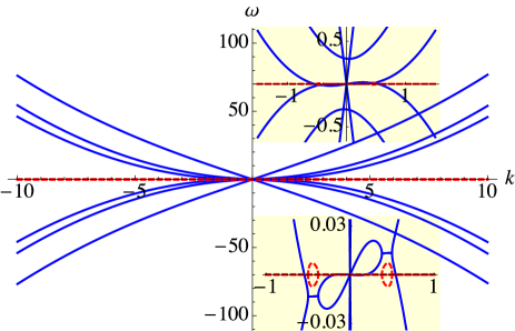
Figure 6: (Color online) Band diagram (frequency as a function of wave vector) for phonons propagating on top of an ($n=0$)–type cw solution of a ⁸⁷Rb BEC where the $M_{F}=1$ and $M_{F}=-1$ components have wave vectors that differ by $k_{1}-k_{-1}=1$, and amplitudes $2$ and $2.5$. The energies (chemical potentials) come from the real parts of the frequencies ($E=\hbar\mathrm{Re}[\omega]$), which are shown as solid lines; and the MI comes from the imaginary parts of the frequencies, which are dotted lines. All quantities in the figure are dimensionless; see Eqs. (3).

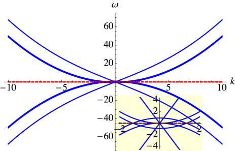
Figure 7: (Color online) Band diagram (frequency as a function of wave vector) for phonons propagating on top of an ($n=0$)–type cw solution of a ²³Na BEC where the $M_{F}=1$ and $M_{F}=-1$ spin components have the same wave vectors and amplitudes $2$ and $2.5$. The energies (chemical potentials) come from the real parts of the frequencies ($E=\hbar\mathrm{Re}[\omega]$), which are shown as solid lines. The imaginary parts of the frequencies, shown as dotted lines, which would create MI, are zero. All quantities in the figure are dimensionless; see Eqs. (3).

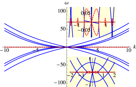
Figure 8: (Color online) Band diagram (frequency as a function of wave vector) for phonons propagating on top of an ($n=0$)–type cw solution of a ²³Na BEC where the $M_{F}=1$ and $M_{F}=-1$ components have wave vectors that differ by $k_{1}-k_{-1}=1$, and amplitudes $2$ and $2.5$. The energies (chemical potentials) come from the real parts of the frequencies ($E=\hbar\mathrm{Re}[\omega]$), which are shown as solid lines; and the MI comes from the imaginary parts of the frequencies, which are dotted lines. All quantities in the figure are dimensionless; see Eqs. (3).

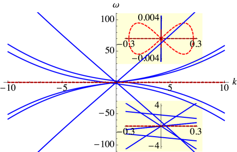
Figure 9: (Color online) Band diagram (frequency as a function of wave vector) for phonons propagating on top of an ($n=1$)–type cw solution of a ²³Na BEC where the $M_{F}=1$ and $M_{F}=-1$ components have wave vectors that differ by $k_{1}-k_{-1}=1$, and amplitudes $2$ and $2.5$. The energies (chemical potentials) come from the real parts of the frequencies ($E=\hbar\mathrm{Re}[\omega]$), which are shown as solid lines; and the MI comes from the imaginary parts of the frequencies, which are dotted lines. All quantities in the figure are dimensionless; see Eqs. (3).

III.4 Peak modulational instabilities

Modulational instabilities are often more consequential than stable sound waves because amplification can make them grow from weak to strong, and the phonons with the largest amplification tend to dominate after sufficient propagation. Let us then look at the maximum MI (the wave number at which the imaginary part of the frequency is largest, or max${}_{j,k}[\omega_{j}(k)]$, as well as the value of the wave number $k$ at which the maximum is found). Since we are now examining maxima rather than the entire band diagrams, we can look at larger sections (more dimensions of) the parameter space. We plot the maximum MI over two-dimensional cross-sections of the cw parameter space (rather than, as above, for one cw at a time). Figures 12–15 show the maximum MI against the amplitudes (square root of the particle density) of the $M_{F}=\pm 1$ and fields, for particular differences in wave numbers ($k_{1}-k_{-1}=0,1$ in dimensionless units), for the different classes of cw solutions (CNLS, $n=0$, or $n=1$), for ²³Na (which is anti-ferromagnetic, with $c_{2}>0$) and ⁸⁷Rb (which is ferromagnetic, with $c_{2}<0$). Quadratic Zeeman splitting is zero in these figures.

Figure 10 shows the peak MI for the cws of a ⁸⁷Rb BEC with identical wave vectors in the spin $M_{F}=\pm 1$ components, $k_{1}=k_{-1}$, and zero quadratic Zeeman splitting. See Fig. 1 for the dispersion curves underlying one point in this plot.

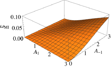
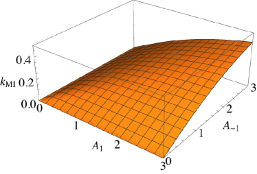
Figure 10: Maximum MI of the CNLS–type cws (zero $M_{F}=0$ particle density) of a ⁸⁷Rb BEC, as a function of the amplitudes of the $M_{F}=\pm 1$ fields, where the spin components have identical wave vectors $k_{1}=k_{-1}$, and quadratic Zeeman splitting is zero. Part (a) shows the peak MI values, and the Part (b) shows the wave vectors at which the maxima occur. All quantities in the figure are dimensionless; see Eqs. (3).

Figure 11 shows the peak modulational instabilities for the cws of a ⁸⁷Rb BEC with wave vectors in the spin $M_{F}=\pm 1$ components with (in dimensionless units) unit difference $k_{1}-k_{-1}=1$, and zero quadratic Zeeman splitting. See Fig. 2 for the dispersion curves underlying one point in this plot.

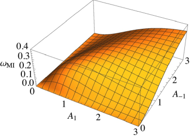
Figure 11: Maximum MI of the CNLS–type cws (zero $M_{F}=0$ particle density) of a ⁸⁷Rb BEC, as a function of the amplitudes of the $M_{F}=\pm 1$ fields, where the spin components have wave vectors that differ by $k_{1}-k_{-1}=1$, and quadratic Zeeman splitting is zero. Part (a) shows the peak MI values, and Part (b) shows the wave vectors at which the maxima occur. All quantities in the figure are dimensionless; see Eqs. (3).

Coupled NLS–type cws for a ²³Na BEC with identical wave numbers $k_{1}=k_{-1}$ and without quadratic Zeeman splitting have zero MI (cf. Fig. 3) for all values of the amplitudes $A_{1}$, $A_{-1}$. Figure 12 shows the peak modulational instabilities for the cws of a ²³Na BEC with spin components with a unit difference between the wave numbers of the spin $M_{F}=\pm 1$ components, $k_{1}-k_{-1}=1$, and zero quadratic Zeeman splitting. See Fig. 4 for the dispersion curves underlying one point in this plot.

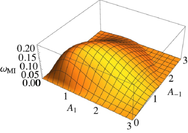
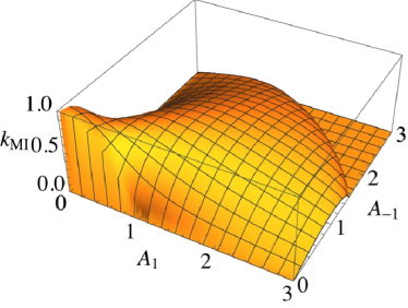
Figure 12: Maximum MI of CNLS–type (zero $M_{F}=0$ particle density) cws of a ²³Na BEC, as a function of the amplitudes of the $M_{F}=\pm 1$ fields, where the spin components have wave vectors that differ by $k_{1}-k_{-1}=1$, and quadratic Zeeman splitting is zero. Part (a) shows the peak MI values, and Part (b) shows the wave vectors at which the maxima occur. All quantities in the figure are dimensionless; see Eqs. (3).

Next, let us show peak MI data for cross-sections of the parameter space for the $n=0$ family of cw solutions, i.e., cws in which $A_{0}$, the square root of the $M_{F}=0$ particle density, is as in Eq. (11), with even-valued $n$. The ($n=0$)–type cws for a ⁸⁷Rb BEC with identical wave vectors in the spin $M_{F}=\pm 1$ components, $k_{1}=k_{-1}$, and zero quadratic Zeeman splitting show vanishing MI at all values of the spin $M_{F}=\pm 1$ amplitudes $A_{\pm 1}$. See Fig. 5 for the dispersion curves underlying one point in the parameter space, and note that the phonon band diagram is real-valued everywhere. In contrast, the corresponding cw but with wave numbers that are not all the same is subject to MI. Figure 13 shows the peak MI for cws of a ⁸⁷Rb BEC with wave vectors in the spin $M_{F}=\pm 1$ components with (in dimensionless units) unit difference $k_{1}-k_{-1}=1$, and zero quadratic Zeeman splitting. See Fig. 6 for the dispersion curves underlying one point in this plot.

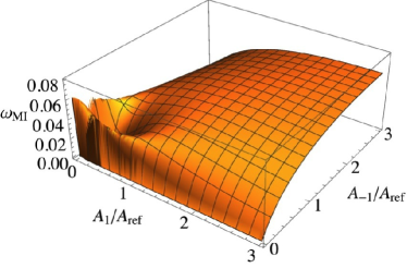
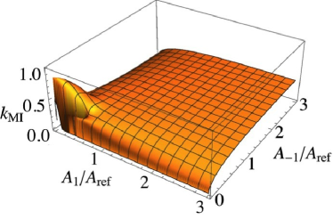
Figure 13: Maximum MI of ($n=0$)–type cws of a ⁸⁷Rb BEC, as a function of the amplitudes of the $M_{F}=\pm 1$ fields, where the spin components have wave vectors that differ by $k_{1}-k_{-1}=1$, and quadratic Zeeman splitting is zero. The (dimensionless) reference amplitude for this plot is $A_{\mathrm{ref}}\equiv\sqrt{|[\hbar^{2}(k_{1}-k_{-1})^{2}/(8m)+qB^{2}]/c_{2}|}=(8|c_{2}|)^{-1/2}\approx 5.103$. Part (a) shows the peak MI values, and Part (b) shows the wave vectors at which the maxima occur. All quantities in the figure are dimensionless; see Eqs. (3).

Next, consider the ($n=0$)–type cw for a ²³Na BEC with identical wave vectors in the spin $M_{F}=\pm 1$ components, $k_{1}=k_{-1}$, and zero quadratic Zeeman splitting. The numerical spectral analysis shows that the MI for all these cws is nil for all values of the spin $M_{F}=\pm 1$ amplitudes $A_{\pm 1}$. See Fig. 7 for the dispersion curves underlying one point in this plot.

Figure 14 shows the peak MI for cws of a ²³Na BEC with a unit difference between the wave numbers of the spin $M_{F}=\pm 1$ components, $k_{1}-k_{-1}=1$, and zero quadratic Zeeman splitting. See Fig. 8 for the dispersion curves underlying one point in this plot.

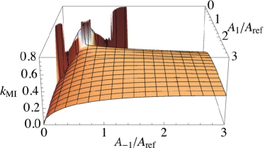
Figure 14: Maximum MI of ($n=0$)–type cws of a ²³Na BEC, as a function of the amplitudes of the $M_{F}=\pm 1$ fields, where the spin components have wave vectors that differ by $k_{1}-k_{-1}=1$, and quadratic Zeeman splitting is zero. The (dimensionless) reference amplitude for this plot is $A_{\mathrm{ref}}\equiv\sqrt{|[\hbar^{2}(k_{1}-k_{-1})^{2}/(8m)+qB^{2}]/c_{2}|}=(8c_{2})^{-1/2}\approx 2.368$. Part (a) the peak MI values, and Part (b) shows the wave vectors at which the maxima occur. All quantities in the figure are dimensionless; see Eqs. (3).

Last in this series, let us show peak MI data for cross-sections of the parameter space for the $n=1$ family of cw solutions, i.e., cws in which $A_{0}$, the square root of the $M_{F}=0$ particle density, is as in Eq. (11), with odd $n$. Figure 15 shows the peak MI for ($n=1$)–type cws of a ²³Na BEC with spin components with a unit difference between the wave numbers of the spin $M_{F}=\pm 1$ components, $k_{1}-k_{-1}=1$, and zero quadratic Zeeman splitting. See Fig. 9 for the dispersion curves underlying one point in this plot.

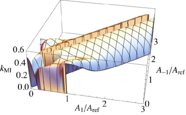
Figure 15: Maximum MI of ($n=1$)–type cws of a ²³Na BEC, as a function of the amplitudes of the $M_{F}=\pm 1$ fields, where the spin components have wave vectors that differ by $k_{1}-k_{-1}=1$, and quadratic Zeeman splitting is zero. The (dimensionless) reference amplitude for this plot is $A_{\mathrm{ref}}\equiv\sqrt{|[\hbar^{2}(k_{1}-k_{-1})^{2}/(8m)+qB^{2}]/c_{2}|}=(8c_{2})^{-1/2}\approx 2.368$. Part (a) shows the peak MI values, and Part (b) shows the wave vectors at which the maxima occur. All quantities in the figure are dimensionless; see Eqs. (3).

The figures are consistent with the well-known fact that there are no modulational instabilities when there is only one spin component in an attractive BEC Bogolubov.1947 ; BespalovTalanov.1966 ; Agrawal.2001 .

Figure 10 confirms that cws in ⁸⁷Rb without $M_{F}=0$ particles are modulationally unstable even for the case in which all the wave numbers of the cws’ spin components are the same. Comparison with Fig. 11 shows that a difference in the wave numbers of the $M_{F}=\pm 1$ fields increases the MI, mostly at low particle densities. Differences in the wave numbers also increase the values of the wave numbers at which the MI is fastest. At higher particle densities, the effects of the wave number differences become less important, and the MI approaches the values of those of the cws with identical wave numbers in all spin components.

CWs in ²³Na without $M_{F}=0$ particles are stable when all the wave numbers of the spin components are the same (no surface plot of the maximum MI is displayed because this is identically zero). Figure 12 shows that cw solutions of ²³Na without $M_{F}=0$ particles and with non-zero difference in the wave vectors of the different spin components, are modulationally unstable at low particle densities, but become stable at larger particle densities For cw solutions with $M_{F}=0$ fields with relative phase corresponding to $n=0$, MI is zero when the wave numbers of the spin components are all the same, MI is non-zero when the difference in the wave numbers is non-zero. The effect of differences in the wave number is larger at low particle densities, and smaller at high particle densities. MI for a $n=1$ cw approaches zero when the densities of the spin $M_{F}=\pm 1$ components are almost the same (when the density of the $M_{F}=0$ particles in the cw is greatest), and also when the densities of the spin $M_{F}=\pm 1$ components are as different as is allowed (when the density of the $M_{F}=0$ particles in the cw is lowest). It may be relevant for for experiments that small amounts of particles with spin $M_{F}=0$ particles may destabilize a cw.

IV Instability growth beyond the linear approximation

We carried out direct numerical simulations, forward in time, for cws with initially small amounts of white noise. The full time evolution shows a great many different phenomena, such as collision of phonons on top of the cws and other effects when the system can no longer be considered a perturbed cw. Phonon collisions will be analyzed in a separate article, since to do so properly would require a great deal of space. The dynamics in a system where a cw cannot be discerned is too large and varied a topic to be contained within this article. To better focus on confirmation of the spectral analyses, we show numerical simulations with a spin-dependent nonlinear coefficient $c_{2}$ that is larger than the physical values in ²³Na and ⁸⁷Rb. The fact that in these materials, $c_{2}$ is smaller than $c_{0}$ by two orders of magnitude causes the MI to be weak. With slow growth rates, once the unstable phonons grow to a certain amplitude, they tend to collide with each other before growing very large, and this obscures the MI-induced amplification. Running simulations with larger values of $c_{2}$ allows us to avoid phonon collisions, and to better focus on one phenomenon at a time: confirmation of the MI.

Figures 16-20 show snapshots of a BEC with $c_{2}=100c_{2}(^{87}\mathrm{Rb})=-.4793c_{0}$ that is initially an ($n=0$)–type cw with dimensionless amplitudes $A_{1}=2.5$, $A_{0}=3.1826$, $A_{-1}=2.0$, wave numbers $k_{1}=0.5$, $k_{0}=0$, $k_{-1}=-0.5$, and frequencies $\omega_{1}=10.6861$, $\omega_{0}=10.6722$, $\omega_{-1}=10.6583$, and initial weak white noise. Figure 16 shows the initial spectral particle densities of the fields with spin $M_{F}=1,0,-1$ and MI as a function of wave number. At dimensionless time $t=176.7$, the noise at the modulationally unstable wavelengths has grown, but not to the point that the BEC cannot still be considered as a perturbed cw. Figure 17 shows the amplitudes in real space—the magnitudes and the real and imaginary parts of the fields $\phi_{1,0,-1}$. Figure 18(a) shows the magnetization vector components and $|\phi_{0}|^{2}$, the density of particles of spin $m=0$. The variation in space of the magnetization may be referred to as spin texture (cf. Sadler.2006 ). Figure 18(b) shows the spectral particle densities of the fields with spin $M_{F}=1,0,-1$. At dimensionless time $t=372.9$, the noise has been amplified so much that the cw has been destroyed, as one can see in Fig. 19, which shows the amplitudes (magnitudes and real and imaginary parts) in real space. Figure 20(a) shows the magnetization density vector (spin texture Sadler.2006 ) and $|\phi_{0}|^{2}$, and Fig. 20(b) shows the spectral particle densities of the spin components $M_{F}=1,0,-1$; compare this with the initial noise and the MI spectrum in Fig. 16. The $t=176.7.$ snapshot looks similar to most of the prior development—a cw with amplified noise at the MI wavelengths—except for the magnitude of the amplified noise. At $t=372.9$, the MI has amplified some of the noise to the point that it has destroyed the cw. The BEC is turbulent. It is no longer meaningful here to talk about phonons. The $t=372.9$ snapshot cannot be said to typify the fields past the point at which the cws have been destroyed; there does not seem to be one typical static or statistical state of the BEC after destruction of the cw. Comparison of Figs. 18 and 20 shows that nontrivial textures (rather than a simple sinusoidal pattern) in the transverse components of the magnetization vector is an indication that the underlying perturbed cw has been destroyed. At lower values of $c_{2}$, phonon collisions can play a dominant role while the cw is still intact, and this can change the development of the noise. Effects of phonon collisions will be examined in another article.

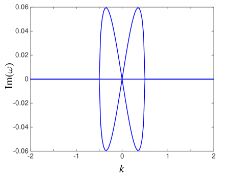
Figure 16: (Color online) Part (a) is the modulational instability band diagram for phonons in a BEC with (dimensionless) parameters $\hbar=1$, $m=1$, $c_{0}=1$, $c_{2}=-.4793$, on top of an ($n=0$)–type cw with amplitudes $A_{1}=2.5$, $A_{0}=3.1826$, $A_{-1}=2.0$, wave numbers $k_{1}=0.5$, $k_{0}=0$, $k_{-1}=-0.5$, and frequencies $\omega_{1}=10.6861$, $\omega_{0}=10.6722$, $\omega_{-1}=10.6583$. Below is the spectral density at the start. The peak in the middle is the cw, and the remainder of the spectrum is statistically flat. All quantities in the figure are dimensionless; see Eqs. (3).

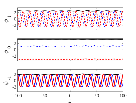
Figure 17: (Color online) Amplitudes of the BEC spin fields $M_{F}=1,0,-1$, in dimensionless variables, at time $t=176.7.$ The magnitudes of the amplitudes are solid lines, the real parts dashed lines, and the imaginary parts dotted. The cw structure is visible, and the amplified noise is also large enough to be visible to the eye. All quantities in the figure are dimensionless; see Eqs. (3).

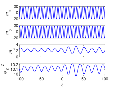
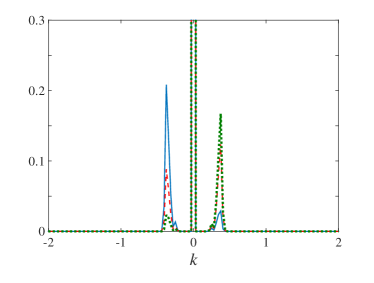
Figure 18: (Color online) Snapshot at dimensionless time $t=176.7$. Part (a) shows the (dimensionless) magnetization components $(m_{x},m_{y},m_{z})$ and the particle density of the $m=0$ spin components, $|\phi_{0}|^{2}$. The pattern is the spin texture. Part (b) shows the squared amplitudes of the fields in momentum-space, i.e., the particle density as a function of wave number, divided by the domain length. The BEC field with spins $M_{F}=1,0,-1$ are represented by solid, dashed, and dotted lined, respectively. All quantities in the figure are dimensionless; see Eqs. (3).

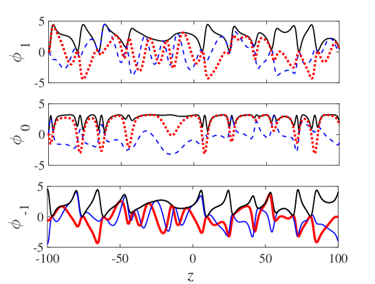
Figure 19: (Color online) Amplitudes of the BEC spin fields $M_{F}=1,0,-1$ at (dimensionless) time $t=372.9$. The magnitudes of the amplitudes are solid lines, the real parts dashed lines, and the imaginary parts dotted. This is a snapshot of dynamical turbulence. The cw has been destroyed by amplified noise, and phonons are no longer helpful in describing the system. All quantities in the figure are dimensionless; see Eqs. (3).

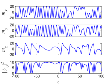
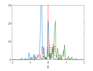
Figure 20: (Color online) Snapshot at dimensionless time $t=372.9$. Part (a) shows the (dimensionless) magnetization components $(m_{x},m_{y},m_{z})$ and the particle density of the $m=0$ spin components, $|\phi_{0}|^{2}$. The pattern is the spin texture. Part (b) shows the squared amplitudes of the fields in momentum-space, i.e., the particle density as a function of wave number, divided by the domain length. The BEC field with spins $M_{F}=1,0,-1$ are represented by solid, dashed, and dotted lines, respectively. All quantities in the figure are dimensionless; see Eqs. (3).

V Summary and Conclusions

We examined the dynamics of sound waves (phonons, acoustic waves, Bogoliubov excitations) in $F=1$ spinor BECs propagating on top of the most general cw solutions. We focused more on cws with non-vanishing $M_{F}=0$ spin components, since this does not have an analog in optics and consequently has not been thoroughly investigated. Emphasis was placed on ²³Na (which is anti-ferromagnetic) and ⁸⁷Rb (which is ferromagnetic), both of which have repulsive nonlinearities.

At any given wave number, the phonons on top of a cw background can take up to six distinct eigenvalues (frequencies or chemical potentials), each with its own eigenvector (i.e., a specific mixture of $M_{F}=1,0,-1$ spin components). We showed the band diagrams (plots of phonon frequencies against wave number) for representative cases of each of the different supported types of cws, for ²³Na and ⁸⁷Rb. Many of the cws are modulationally unstable, i.e., have frequencies with imaginary parts over some range of wave numbers. Perhaps unexpectedly, the cws with non-vanishing $M_{F}=0$ components tend to be less subject to MI than cws with nil particle density for $M_{F}=0$, even though the Hamiltonian densities are higher for the latter. The MIs are in many cases weak and only occur for wave numbers with magnitude up to a given point, beyond which there are no more instabilities (or, equivalently, all phonons with wavelengths smaller than a certain value are stable). Thus, even an “unstable” cw (unstable on an infinite domain), when confined in a toroidal potential, may not support any unstable phonon modes.

Broadly speaking, differences in the wave numbers of the spin components $M_{F}=-1,0,1$ tend to make the cw unstable. All cws without any $M_{F}=0$ particles with nonzero wave number difference are subject to modulational instabilities, even though such a cw in a ²³Na BEC is stable when there is zero difference in the wave numbers. The destabilizing effects of a difference in wave numbers are significant when the particle densities are small, and insignificant when the particle densities are large. All cws with $M_{F}=0$ particles with nonzero wave number difference are subject to modulational instabilities, even though the ($n=0$)–type cws in for both ²³Na and ⁸⁷Rb are stable when there is zero difference in the wave numbers. Note that linear Zeeman splitting may be relevant here, even though it is mathematically trivial. The transformation of variables that eliminates the linear Zeeman terms changes the frequencies and wave numbers of the components with $M_{F}=\pm 1$. Thus a cw in a BEC that feels a linear Zeeman splitting, if it is to have the same frequency (chemical potential) in all original (not transformed) physical components, needs to have different wave numbers for the cw to exist.

Our simulation of the dynamics of BECs confirmed the spectral analyses, i.e., the band diagrams. We observed that MI can lead to exponential growth of noise, and that this can eventually destroy the initial underlying cw and create a spin texture. Nonlinear evolution of the phonons (which includes phonon collisions) is a very large topic, which we will examine in greater detail in subsequent work.

- (1) S. N. Bose, “Plancks Gesetz und Lichtquantenhypothese,” Z. Phys. 26, 178-181 (1924).
- (2) A. Einstein, “Quantentheorie des einatomigen idealen Gases,” Sitzungsber. K. Preuss. Akad. Wiss., Phys. Math. Kl. (1924), 261-267.
- (3) A. Einstein, “Quantentheorie des einatomigen idealen Gases. 2. Abhandlung,” Sitzungsber. K. Preuss. Akad. Wiss., Phys. Math. Kl. (1925), 3-14.
- (4) M. H. Anderson, J. R. Ensher, M. R. Matthews, C. E. Wieman, and E. A. Cornell, “Observation of Bose-Einstein Condensation in a Dilute Atomic Vapor,” Science 269, 198-201 (1995).
- (5) K. B. Davis, M.-O. Mewes, M. R. Andrews, N. J. van Druten, D. S. Durfee, D. M. Kurn, and W. Ketterle, “Bose-Einstein Condensation in a Gas of Sodium Atoms”, Phys. Rev. Lett. 75, 3969 (1995).
- (6) R. P. Feynman, “Quantum Mechanical Computers,” Found. Phys. 16, 507-531 (1986).
- (7) J. I. Cirac and P. Zoller, “Goals and opportunities in quantum simulation,” Nat. Phys. 8, 264 266 (2012).
- (8) O. Lahav, A. Itah, A. Blumkin, C. Gordon, S. Rinott, A. Zayats, and J. Steinhauer, “Realization of a Sonic Black Hole Analog in a Bose-Einstein Condensate,” Phys. Rev. Lett. 105, 240401 (2010).
- (9) A. V. Gorshkov, M. Hermele, V. Gurarie, C. Xu, P. S. Julienne, J. Ye, P. Zoller, E. Demler, M. D. Lukin, and A. M. Rey, “Two-orbital SU(N) magnetism with ultracold alkaline-earth atoms,” Nat. Phys. 6, 289-295 (2010).
- (10) M. Lewenstein, A. Sanpera, and V. Ahufinger, Ultracold Atoms in Optical Lattices: Simulating quantum many-body systems (Oxford University Press, Oxford, 2012).
- (11) H. Saito, Y. Kawaguchi, and M. Ueda, “Topological defect formation in a quenched ferromagnetic Bose-Einstein condensates,” Phys. Rev. A 75, 013621 (2007).
- (12) A. Lamacraft, “Quantum Quenches in a Spinor Condensate,” Phys. Rev. Lett. 98, 160404 (2007).
- (13) M. Uhlmann, R. Schutzhold, and U. R. Fischer, “Vortex Quantum Creation and Winding Number Scaling in a Quenched Spinor Bose Gas,” Phys. Rev. Lett. 99, 120407 (2007).
- (14) Y. Kawaguchi and M. Ueda, “Spinor Bose-Einstein condensates,” Phys. Rep. 520, 253 381 (2012).
- (15) S. Burger, K. Bongs, S. Dettmer, W. Ertmer, K. Sengstock, A. Sanpera, G. V. Shlyapnikov, and M. Lewenstein, “Dark Solitons in Bose-Einstein Condensates,” Phys. Rev. Lett. 83, 5198 (1999).
- (16) J. Denschlag, J. E. Simsarian, D. L. Feder, Charles W. Clark, L. A. Collins, J. Cubizolles, L. Deng, E. W. Hagley, K. Helmerson, W. P. Reinhardt, S. L. Rolston, B. I. Schneider, and W. D. Phillips, “Generating Solitons by Phase Engineering of a Bose-Einstein Condensate,” Science 287, 97-101 (2000).
- (17) L. Li, Z. Li, B. A. Malomed, D. Mihalache, and W. M. Liu, “Exact soliton solutions and nonlinear modulation instability in spinor Bose-Einstein condensates,” Phys. Rev. A 72, 033611 (2005).
- (18) L. E. Sadler, J. M. Higbie, S. R. Leslie, M. Vengalattore, and D. M. Stamper-Kurn, “Spontaneous symmetry breaking in a quenched ferromagnetic spinor Bose-Einstein condensate,” Nature (London) 443, 312-315 (2006).
- (19) D. G. Fried, T. C. Killian, L. Willmann, D. Landhuis, S. C. Moss, D. Kleppner, and T. J. Greytak, “Bose-Einstein Condensation of Atomic Hydrogen,” Phys. Rev. Lett. 81, 3811 (1998).
- (20) C. C. Bradley, C. A. Sackett, and R. G. Hulet, “Bose-Einstein Condensation of Lithium: Observation of Limited Condensate Number,” Phys. Rev. Lett. 78, 985-989 (1997).
- (21) M. V. Simkin and E. G. D. Cohen, “Magnetic properties of a Bose-Einstein condensate,” Phys. Rev. A 59, 1528-1532 (1999).
- (22) G. Modugno, G. Ferrari, G. Roati, R. J. Brecha, A. Simoni, and M. Inguscio, “Bose-Einstein Condensation of Potassium Atoms by Sympathetic Cooling,” Science 294, 1320-1322 (2001).
- (23) A. Griesmaier, J. Werner, S. Hensler, J. Stuhler, and T. Pfau, “Bose-Einstein Condensation of Chromium,” Phys. Rev. Lett. 94, 160401 (2005).
- (24) S. Stellmer, M. K. Tey, B. Huang, R. Grimm, and F. Schreck, “Bose-Einstein Condensation of Strontium,” Phys. Rev. Lett. 103, 200401 (2009).
- (25) S. L. Cornish, N. R. Claussen, J. L. Roberts, E. A. Cornell, and C. E. Wieman, “Stable 85Rb Bose-Einstein Condensates with Widely Tunable Interactions,” Phys. Rev. Lett. 85, 1795 (2000).
- (26) T. Weber, J. Herbig, M. Mark, H.-C. Nagerl, and R. Grimm, “Bose-Einstein Condensation of Cesium,” Science 299, 232-235 (2003).
- (27) M. Lu, N. Q. Burdick, S. H. Youn, and B. L. Lev, “Strongly Dipolar Bose-Einstein Condensate of Dysporium,” Phys. Rev. Lett. 107, 190401 (2011).
- (28) T. Fukuhara, S. Sugawa, and Y. Takahashi, “Bose-Einstein condensation of an ytterbium isotope,” Phys. Rev. A 76, 051604 (2007).
- (29) M. D. Barrett, J. A. Sauer, and M. S. Chapman, “All-Optical Formation of an Atomic Bose-Einstein Condensate,” Phys. Rev. Lett. 87, 010404 (2001).
- (30) M.-S. Chang, C. D. Hamley, M. D. Barrett, J. A. Sauer, K. M. Fortier, W. Zhang, L. You, and M. S. Chapman, “Observation of Spinor Dynamics in Optically Trapped 87Rb Bose-Einstein Condensates,” Phys. Rev. Lett. 92, 140403 (2004).
- (31) Q. Beaufils, R. Chicireanu, T. Zanon, B. Laburthe-Tolra, E. Marechal, L. Vernac, J.-C. Keller, and O. Gorceix, “All-optical production of chromium Bose-Einstein condensates,” Phys. Rev. A 77, 061601R (2008).
- (32) S. R. Leslie, J. Guzman, M. Vengalattore, J. D. Sau, M. L. Cohen, and D. M. Stamper-Kurn, “Amplification of fluctuations in a spinor Bose-Einstein condensate,” Phys. Rev. A 79, 043631 (2009).
- (33) N. P. Robins, W. Zhang, E. A. Ostrovskaya, and Y. S. Kivshar, “Modulational instability of spinor condensates,” Phys. Rev. A 64, 021601(R) (2001).
- (34) V. V. Konotop and M. Salerno, “Modulational instability in Bose-Einstein condensates in optical lattices,” Phys. Rev. A 65, 021602(R) (2002).
- (35) W. Zhang, D. L. Zhou, M. S. Chang, M. S. Chapman, and L. You, “Dynamical Instability and Domain Formation in a Spin-1 Bose-Einstein Condensate,” Phys. Rev. Lett. 95, 180403 (2005).
- (36) M. Kunimi, “Metastable spin textures and Nambu-Goldstone modes of a ferromagnetic spin-1 Bose-Einstein condensate confined in a ring trap,” Phys. Rev. A 90, 063632 (2014).
- (37) W. Zhang, D. L. Zhou, M. S. Chang, M. S. Chapman, and L. You, “Coherent spin mixing dynamics in a spin-1 atomic condensate,” Phys. Rev. A 72, 013602 (2005).
- (38) J. Mur-Petit, “Spin dynamics and structure formation in a spin-1 condensate in a magnetic field,” Phys. Rev. A 79, 063603 (2009).
- (39) R. S. Tasgal and Y. B. Band, “Continuous-wave solutions in spinor Bose-Einstein condensates,” Phys. Rev. A 87, 023626 (2013).
- (40) M.-O. Mewes, M. R. Andrews, N. J. van Druten, D. M. Kurn, D. S. Durfee, C. G. Townsend, and W. Ketterle, “Collective Excitations of a Bose-Einstein Condensate in a Magnetic Trap,” Phys. Rev. Lett. 77, 988 (1996).
- (41) M. R. Andrews, D. M. Kurn, H.-J. Miesner, D. S. Durfee, C. G. Townsend, S. Inouye, and W. Ketterle, “Propagation of Sound in a Bose-Einstein Condensate,” Phys. Rev. Lett. 79, 553-556 (1997).
- (42) M. R. Andrews, D. M. Stamper-Kurn, H.-J. Miesner, D. S. Durfee, C. G. Townsend, S. Inouye, and W. Ketterle, “Erratum: Propagation of Sound in a Bose-Einstein Condensate,” Phys. Rev. Lett. 80, 2967 (1998).
- (43) J. Steinhauer, R. Ozeri, N. Katz, and N. Davidson, “Excitation Spectrum of a Bose-Einstein Condensate,” Phys. Rev. Lett. 88, 120407 (2002).
- (44) R. Ozeri, N. Katz, J. Steinhauer, and N. Davidson, “Colloquium: Bulk Bogoliubov excitations in a Bose-Einstein condensate,” Rev. Mod. Phys. 77, 187-205 (2005).
- (45) N. Bogolubov, “On the Theory of Superfluidity,” Izv. Akad. Nauk. SSSR Ser. Fiz. 11, 77-90 (1947) [J. Phys. (Moscow) 11, 23-32 (1947)].
- (46) V. I. Bespalov and V. I. Talanov, “Filamentary Structure of Light Beams in Nonlinear Media,” Pis’ma Zh. Eksp. Teor. Fiz. 3, 471-476 (1966) [JETP Lett. 3, 307-310 (1966)].
- (47) T. B. Benjamin and J. E. Feir, “The disintegration of wave trains on deep water. Part 1. Theory,” J. Fluid Mech. 27, 417-430 (1967)
- (48) G. P. Agrawal, Applications of Nonlinear Fiber Optics (Academic, New York, 2001).
- (49) T. Ohmi and K. Machida, “Bose-Einstein Condensation with Internal Degrees of Freedom in Alkali Atom Gases,” J. Phys. Soc. Jpn. 67, 1822-1825 (1998).
- (50) T.-L. Ho, “Spinor Bose Condensates in Optical Traps,” Phys. Rev. Lett. 81, 742-745 (1998).
- (51) D. M. Stamper-Kurn and M. Ueda, “Spinor Bose gases: Symmetries, magnetism, and quantum dynamics,” Rev. Mod. Phys. 85, 1191 (2013).
- (52) M. Olshanii, “Atomic Scattering in the Presence of an External Confinement and a Gas of Impenetrable Bosons,” Phys. Rev. Lett. 81, 938-941 (1998).
- (53) T. Bergeman, M. G. Moore, and M. Olshanii, “Atom-Atom Scattering under Cylindrical Harmonic Confinement: Numerical and Analytic Studies of the Confinement Induced Resonance,” Phys. Rev. Lett. 91, 163201 (2003).
- (54) M.-S. Chang, Q. Qin, W. Zhang, L. You, and M. S. Chapman, “Coherent spinor dynamics in a spin-1 Bose condensate,” Nat. Phys. 1, 111-116 (2005).
- (55) N. N. Klausen, J. L. Bohn and C. H. Greene, “Nature of spinor Bose-Einstein condensates in rubidium,” Phys. Rev. A 64, 053602 (2001).
- (56) E. G. M. van Kempen, S. J. J. M. F. Kokkelmans, D. J. Heinzen, and B. J. Verhaar, “Interisotope Determination of Ultracold Rubidium Interactions from Three High-Precision Experiments,” Phys. Rev. Lett. 88, 093201 (2002).
- (57) S. V. Manakov, “On the theory of two-dimensional stationary self-focusing of electromagnetic waves,” Zh. Eksp. Teor. Fiz. 65, 505-516 (1973) [Sov. Phys.-JETP 38, 248-253 (1974)].
- (58) K. Nakkeeran, K. Porsezian, P. Shanmugha Sundaram, and A. Mahalingam, “Optical Solitons in N-Coupled Higher Order Nonlinear Schrödinger Equations,” Phys. Rev. Lett. 80, 1425-1428 (1998).
- (59) J. Ieda, T. Miyakawa, and M. Wadati, “Exact Analysis of Soliton Dynamics in Spinor Bose-Einstein Condensates,” Phys. Rev. Lett. 93, 194102 (2004).
- (60) M. Wadati and N. Tsuchida, “Wave Propagations in the Spinor Bose-Einstein Condensates,” J. Phys. Soc. Japan 75, 014301 (2006).
- (61) J. Ieda and M. Wadati, “Nonlinear Dynamics of Spin Structure in Confined Bose-Einstein Condensates,” J. Low Temp. Phys. 148, 405-410 (2007).
- (62) V. E. Zakharov and A. B. Shabat, “Exact theory of two-dimensional self-focusing and one-dimensional self-modulation of waves in nonlinear media,” Zh. Eksp. Teor. Fiz. 61, 118-134 (1971) [Sov. Phys. JETP 34, 62-69 (1972)].
- (63) V. E. Zakharov and A. B. Shabat, “Interaction between solitons in a stable medium,” Zh. Eksp. Teor. Fiz. 64, 1627-1639 (1973) [Sov. Phys. JETP 37, 823-828 (1973)].
- (64) J. Yang, Nonlinear Waves in Integrable and Nonintegrable Systems, (SIAM, Philadelphia, 2010).
- (65) S. Gupta, K. W. Murch, K. L. Moore, T. P. Purdy, and D. M. Stamper-Kurn, “Bose-Einstein Condensation in a Circular Waveguide,” Phys. Rev. Lett. 95, 143201 (2005).
- (66) S. E. Olson, M. L. Terraciano, M. Bashkansky, and F. K. Fatemi, “Cold-atom confinement in an all-optical dark ring trap,” Phys. Rev. A 76, 061404(R) (2007).
- (67) I. Lesanovsky and W. von Klitzing, “Time-Averaged Adiabatic Potentials: Versatile Matter-Wave Guides and Atom Traps,” Phys. Rev. Lett. 99, 083001 (2007).
- (68) K. Henderson, C. Ryu, C. MacCormick, and M. G. Boshier, “Experimental demonstration of painting arbitrary and dynamic potentials for Bose-Einstein condensates,” New J. Phys. 11, 043030 (2009).
- (69) C. Ryu, M. F. Andersen, P. Clade, V. Natarajan, K. Helmerson, and W. D. Phillips, “Observation of Persistent Flow of a Bose-Einstein Condensate in a Toroidal Trap,” Phys. Rev. Lett. 99, 260401 (2007).
- (70) C. R. Menyuk, “Nonlinear Pulse Propagation in Birefringent Optical Fiber,” IEEE J. Quantum Electron. QE-23, 174-176 (1987).
- (71) G. P. Agrawal, “Modulation Instability Induced by Cross-Phase Modulation,” Phys. Rev. Lett. 59, 880-883 (1987).
- (72) G. P. Berman, A. Smerzi, and A. R. Bishop, “Quantum Instability of a Bose-Einstein Condensate with Attractive Interaction,” Phys. Rev. Lett. 88, 120402 (2002).
- (73) G. Huang, X.-Q. Li, and J. Szeftel, “Second-harmonic generation of Bogoliubov excitations in a two-component Bose-Einstein condensate,” Phys. Rev. A 69, 065601 (2004).
- (74) C. K. Law, C. M. Chan, P. T. Leung, and M.-C. Chu, “Critical velocity in a binary mixture of moving Bose condensates,” Phys. Rev. A 63, 063612 (2001).
- (75) F. Tsitoura, V. Achilleos, B. A. Malomed, D. Yan, P. G. Kevrekidis, and D. J. Frantzeskakis, “Matter-wave solitons in the counterflow of two immiscible superfluids,” Phys. Rev. A 87, 063624 (2013).