Anomalous Behavior of the Magnetization Process of the $S=1/2$ Kagome-Lattice Heisenberg Antiferromagnet at One-Third Height of the Saturation

Abstract

The magnetization process of the $S=1/2$ Heisenberg antiferromagnet on the kagome lattice is studied by the numerical-diagonalization method. We successfully obtain a new result of the magnetization process of a 42-site cluster in the entire range. Our analysis clarifies that the critical behavior around one-third of the height of the saturation is different from the typical behavior of the well-known magnetization plateau in two-dimensional systems. We also examine the effect of the $\sqrt{3}\times\sqrt{3}$-type distortion added to the kagome lattice. We find at one-third of the height of the saturation in the magnetization process that the undistorted kagome point is just the boundary between two phases that show their own properties that are different from each other. Our results suggest a relationship between the anomalous critical behavior at the undistorted point and the fact that the undistorted point is the boundary.

1 Introduction

Various characteristics of a magnetic material are included in its magnetization process. They provide us with useful information to understand the properties of a material well. Among such characteristic behaviors, the phenomenon of magnetization plateaux has long attracted the attention of many experimental and theoretical researchers. A magnetization plateau is the behavior of the appearance of a region of magnetic field in a magnetization process where the magnetization does not increase even with an increase in the magnetic field, in contrast to the fact that a normal magnetization process shows a smooth and significant increase in the magnetization with an increase in the magnetic field. The magnetization plateau originates from the existence of an energy gap between states with different magnetizations; the nonzero gap occurs owing to the formation of an energetically stable quantum spin state. The field dependence of magnetization just outside the plateau generally originates from the nature of the density of states determined from the parabolic dispersion of states next to the energy gap, where the field dependence of magnetization shows a characteristic exponent $\delta$ defined in the form of

$$|m-m_{\rm c}|\sim|h-h_{\rm c}|^{1/\delta}.$$ (1)

Therefore, this exponent is determined by the spatial dimension of the system: for example, $\delta=1$ for the two-dimensional system.

Under these circumstances, it is an interesting case if it has attracted the attention of many physicists studying magnetism, in terms of whether the magnetization plateau is formed and how the magnetization behaves as a function of the magnetic field outside the plateau, that is, the $S=1/2$ Heisenberg antiferromagnet on the kagome lattice. In recent years, the kagome-lattice antiferromagnet has attracted increasing interest not only as a theoretical toy model but also from the viewpoint of discoveries of several realistic materials: herbertsmithite[1, 2], volborthite[3, 4], and vesignieite[5, 6]. Since the kagome-lattice antiferromagnet is a typical two-dimensional frustrated system, most theoretical studies have been carried out mainly by the basis of the numerical-diagonalization method[7, 8, 9, 10, 11, 12, 13, 14, 15, 16, 17, 18, 19, 20]. The brief behavior of the magnetization process of the kagome-lattice antiferromagnet was clarified in Ref. References, which showed the existence of the magnetization plateau at one-third of the height of the saturation. This result was supported by Ref. References. However, these studies did not focus much on the behavior just outside of the plateau. References References and References, on the other hand, pointed out that the behavior outside of the state of this height is different from that of the well-known magnetization plateau explained above, and that the width of the finite-size step at this height possibly vanishes in the thermodynamic limit. In particular, Ref. References showed anomalous critical exponents for the behavior just outside of the one-third magnetization state, which are different from the exponent $\delta=1$ for the typical magnetization plateau of a two-dimensional system. The authors of Ref. References, however, considered that the width of the plateau survives from the studies based on the model with easy-axis exchange anisotropies[10, 13], although the authors did not mention the behavior just outside of the plateau.

Recently, on the other hand, there have been an increasing number of studies where the density matrix renormalization group (DMRG) calculations are applied to the kagome-lattice antiferromagnet[21, 22, 23, 24]. By the grand canonical analysis[25] based on their DMRG calculations applied to the kagome-lattice antiferromagnet, Ref. References reported the existence of the magnetization plateau at the one-third height together with those at the one-ninth, five-ninth, and seven-ninth heights, although the authors did not discuss the behavior just outside of the plateaux; the author of Ref. References also proposed quantum spin states with a nine-site structure as the states characterizing the plateaux. If such a state is stably realized at the one-third height, the above argument of the relationship between the parabolic dispersion and the critical exponent $\delta$ might give a conclusion that the upper and lower-side dispersions give the normal critical behavior in the field dependence of magnetization just outside the plateau.

The purpose of this paper is to study the true behavior of the magnetization process for the $S=1/2$ Heisenberg antiferromagnet on the kagome lattice with as much effort as possible on the basis of numerical-diagonalization data. We tackle this issue from the following two routes. One is to examine our new result of the magnetization process for a 42-site cluster. To the best of our knowledge, this is the first report on the magnetization process of this size in the $S=1/2$ model within the entire range from the zero magnetization to the saturation[26]. Note here that this large-scale calculation has been carried out using the K computer, Kobe, Japan. The other route is to examine the change that occurs by adding a distortion to the ideal undistorted kagome lattice. In this study, we investigate the case of the $\sqrt{3}\times\sqrt{3}$ type. From these results, we try to clarify the reason for the discrepancy between the numerical-diagonalization and DMRG studies concerning the behavior at the one-third height.

This paper is organized as follows. In the next section, the model that we study here is introduced. The method and analysis procedure are also explained. The third section is devoted to the presentation and discussion of our results. Our results including new data for the 42-site cluster clearly indicate anomalous critical exponents for the field dependence of magnetization just outside the plateau. Examining the effect of the distortion in the kagome lattice clarifies that the undistorted point is just at the boundary between two phases, which are different from each other. In the final section, we present our conclusion together with some remarks and discussion.

2 Model Hamiltonians, Method, and Analysis

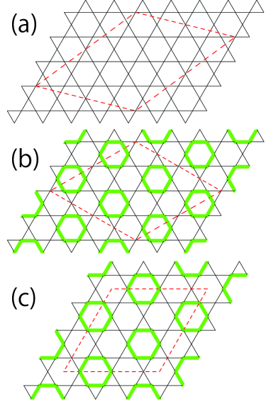
Figure 1: (Color) Finite-size clusters of the kagome-lattice antiferromagnet with and without the $\sqrt{3}\times\sqrt{3}$ distortion. In (a), a cluster with $N_{\rm s}=42$ on the undistorted kagome lattice is illustrated by the parallelogram of red broken lines. The $\sqrt{3}\times\sqrt{3}$ distorted kagome lattice is shown in (b) and (c) by the green thick lines and black thin lines. The finite-size clusters of $N_{\rm s}=36$ and $N_{\rm s}=27$ are presented by the rhombus of red broken lines in (b) and (c), respectively.

The Hamiltonian that we study in this research is given by ${\cal H}={\cal H}_{0}+{\cal H}_{\rm Zeeman}$, where

$${\cal H}_{0}=\sum_{\langle i,j\rangle}J\mbox{\boldmath$S$}_{i}\cdot\mbox{\boldmath$S$}_{j},$$ (2)

for the model on the undistorted kagome lattice. Particularly, we examine a cluster with 42 sites of spins shown in Fig. 1(a). We also study

$${\cal H}_{0}=\sum_{\langle i,j\rangle\in{\rm black\ bonds}}J_{\rm 1}\mbox{\boldmath$S$}_{i}\cdot\mbox{\boldmath$S$}_{j}+\sum_{\langle i,j\rangle\in{\rm green\ bonds}}J_{\rm 2}\mbox{\boldmath$S$}_{i}\cdot\mbox{\boldmath$S$}_{j},$$ (3)

for the model on the distorted kagome lattice shown in Figs. 1(b) and 1(c). Hereafter, vertices of thick green hexagons are denoted by $\alpha$ sites and other vertices are denoted by $\beta$ sites. Here, ${\cal H}_{\rm Zeeman}$ is given by

$${\cal H}_{\rm Zeeman}=-h\sum_{j}S_{j}^{z}.$$ (4)

Here, $\mbox{\boldmath$S$}_{i}$ denotes the $S=1/2$ spin operator at site $i$ illustrated by the vertices of the undistorted and distorted kagome lattices. The sum of ${\cal H}_{0}$ runs over all the pairs of spin sites linked by solid lines in Fig. 1. Energies are measured in units of $J$ for the undistorted kagome lattice and $J_{\rm 1}$ for the distorted kagome lattice; hereafter, we set $J=1$ and $J_{\rm 1}=1$. The number of spin sites is denoted by $N_{\rm s}$. We impose the periodic boundary condition for clusters with site $N_{\rm s}$. Note here that the case of $J_{2}/J_{1}=1$ in the Hamiltonian (3) is reduced to the Hamiltonian (2).

We calculate the lowest energy of ${\cal H}_{0}$ in the subspace characterized by $\sum_{j}S_{j}^{z}=M$ by numerical diagonalizations based on the Lanczos algorithm and/or the Householder algorithm. The energy is denoted by $E(N_{\rm s},M)$, where $M$ takes an integer from zero to the saturation value $M_{\rm s}$ ($=SN_{\rm s}$). We often use the normalized magnetization $m=M/M_{\rm s}$. To achieve calculations of large clusters, particularly the case of $N_{\rm s}=42$, some of Lanczos diagonalizations have been carried out using the MPI-parallelized code, which was originally developed in the study of Haldane gaps[27]. The usefulness of our program was confirmed in large-scale parallelized calculations[18, 28].

The magnetization process for a finite-size system is obtained by the magnetization increase from $M$ to $M+1$ at the field

$$h=E(N_{\rm s},M+1)-E(N_{\rm s},M),$$ (5)

under the condition that the lowest-energy state with the magnetization $M$ and that with $M+1$ become the ground state in specific magnetic fields. However, it often happens that the lowest-energy state with the magnetization $M$ does not become the ground state in any field. In this case, the magnetization process around the magnetization $M$ is determined by the Maxwell construction[29, 30].

The critical exponent $\delta$ is a good index for characterizing the universality class of the field-induced phase transitions. To estimate this $\delta$ just outside a specified $m$ in the magnetization process, we use the finite-size scaling developed in Ref. References. Although this method was originally proposed for one-dimensional cases, the validity for two-dimensional cases has been confirmed, for example, in the triangular-lattice antiferromagnet[17]. We first assume the asymptotic form of the system size dependence of the energy to be

$$\frac{1}{N_{\rm s}}E(N_{\rm s},M)\sim\epsilon(m)+C(m)\frac{1}{N_{\rm s}^{\theta}},\ (N_{\rm s}\rightarrow\infty),$$ (6)

where $\epsilon(m)$ is the energy per site. The second term means the leading correction with respect to $N_{\rm s}$. We also assume that $C(m)$ is an analytic function of $m$. In this paper, we focus our attention on the case of $m=1/3$. Thus, the exponents that we want to know are $\delta_{\pm}$ defined in the form of

$$\left|m-\frac{1}{3}\right|\sim\left|h-h_{\rm c\pm}\right|^{1/\delta_{\pm}},$$ (7)

where the critical fields are defined as

$$h_{\rm c\pm}=\pm\lim_{N_{\rm s}\rightarrow\infty}\left[E\left(N_{\rm s},\frac{M_{\rm s}}{3}\pm 1\right)-E\left(N_{\rm s},\frac{M_{\rm s}}{3}\right)\right].$$ (8)

If we define the quantity $f_{\sigma}(N_{\rm s})$ by

$$f_{\pm}(N_{\rm s}) = E\left(N_{\rm s},\frac{M_{s}}{3}\pm 2\right)+E\left(N_{\rm s},\frac{M_{s}}{3}\right)$$ (9)

$$-2E\left(N_{\rm s},\frac{M_{s}}{3}\pm 1\right),$$

the asymptotic forms of $f_{\sigma}(N_{\rm s})$ are expected to be

$$f_{\pm}(N_{\rm s})\sim\frac{1}{N_{\rm s}^{\delta_{\pm}}}+O\left(\frac{1}{N_{\rm s}^{\theta+1}}\right),$$ (10)

where $N_{\rm s}\rightarrow\infty$ as long as we assume Eq. (8). Therefore, it is possible to estimate the exponents $\delta_{+}$ and $\delta_{-}$ from the gradient of the linear fitting in the $\ln(f_{\sigma})$-$\ln(N_{\rm s})$ plot when the condition $\theta+1>\delta_{\sigma}$ holds. In this study, we carry out our analysis of $\delta_{\sigma}$ assuming this condition because the assumption is reasonable from successful estimates of the exponents in two- and one-dimensional systems[31, 17], which are consistent with the relationship between the parabolic dispersion and the critical exponent depending on the spatial dimension.

3 Results and Discussion

3.1 Case of undistorted kagome lattice

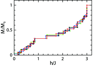
Figure 2: (Color) Magnetization process for the undistorted kagome-lattice antiferromagnet. The results of finite-size clusters for $N_{\rm s}=42$, 39, 36, and 27 are illustrated by red circles, blue triangles, black squares, and green reversed triangles, respectively.

Let us first observe the magnetization process of the $N_{\rm s}=42$ clusters in the undistorted case. The result is shown in Fig. 2 together with the magnetization process for the $N_{\rm s}=39$ cluster, that for the $N_{\rm s}=36$ cluster, and that for the $N_{\rm s}=27$ cluster. Note here that although the clusters for $N_{\rm s}=27$, 36, and 39 are rhombic, the $N_{\rm s}=42$ cluster is not rhombic. Even in such a situation of the anisotropy in a two-dimensional lattice, it is sufficiently worth examining the result of a size that has not been reached in previous studies. In particular, the $N_{\rm s}=42$ cluster suits the investigation of the behavior at approximately $m=1/3$, although it does not suit the study of the behavior at $m=1/9$, $5/9$, and $7/9$ because $N_{\rm s}/9$ is not an integer. The width of the $N_{\rm s}=42$ step at $m=1/3$, namely, $M=\frac{1}{3}M_{\rm s}$, seems large. The width at $M=\frac{1}{3}M_{\rm s}-1$ is quite small. On the other hand, the width at $M=\frac{1}{3}M_{\rm s}+1$ is large even if one compares it with the width at $M=\frac{1}{3}M_{\rm s}$. These features are common with the clusters of $N_{\rm s}=39$, 36, and 27; one finds that the features do not depend on the system size.

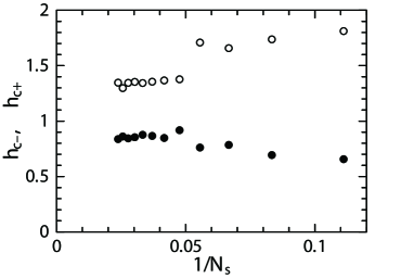
Figure 3: System size dependence of the position of the edges at the height of $m=1/3$ in the magnetization process for the undistorted kagome-lattice antiferromagnet.

To examine the position of the edges of the state at $m=1/3$ in more detail, we plot its system size dependence as a function of $1/N_{\rm s}$; the result is shown in Fig. 3. This figure was originally presented as Fig. 4 in Ref. References; however, the plotted data were limited to cases up to $N_{\rm s}=33$. We additionally plotted the results for larger clusters $N_{\rm s}=36$, 39, and 42. The new datum of $h_{\rm c-}$ for $N_{\rm s}=42$ is quite close to the data for a smaller $N_{\rm s}$. The situation is the same as that for $h_{\rm c+}$. The data for $N_{\rm s}\geq 21$ seem almost independent of $N_{\rm s}$ and seem to converge to different values with each other. In this sense, our new data for $N_{\rm s}=42$ are not the results which suggests that the width $h_{\rm c+}-h_{\rm c-}$ decays and vanishes in the thermodynamic limit. However, there certainly exists a discontinuous size dependence between $N_{\rm s}=18$ and 21. The present new data for $N_{\rm s}=42$ cannot guarantee that a similar discontinuous behavior never happens for $N_{\rm s}>42$. It may be premature to conclude from the numerical-diagonalization data whether the width at $m=1/3$ survives or vanishes in the thermodynamic limit. Another important feature is that, at least for $N_{\rm s}\geq 21$, the size dependence of data in the case when $N_{\rm s}/9$ is an integer is in agreement with that in the case when $N_{\rm s}/9$ is not an integer. If the quantum state at $m=1/3$ forms a nine-site structure, the state becomes stable from the viewpoint of its energy. In the case when $N_{\rm s}/9$ is not an integer, on the other hand, the nine-site structure is partly realized in finite-size clusters; the energies per site may be larger than those in the case when $N_{\rm s}/9$ is an integer. The consequence would lead to the appearance of a difference in data in Fig. 3 between whether $N_{\rm s}/9$ is an integer and is not. However, Fig. 3 does not show such a difference. Thus, it is not reasonable to consider that the state at $m=1/3$ shows the nine-site structure as a long-range order, although a feature of the nine-site structure may survive as a short-range correlation.

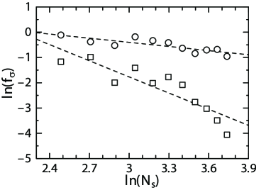
Figure 4: $\ln(f_{\sigma})$ is plotted vs $\ln(N_{\rm s})$ for the undistorted kagome-lattice antiferromagnet. Circles and squares denote the results for $f_{+}$ and $f_{-}$, respectively. The broken lines are the results of the linear fitting in this plot.

Next, let us examine the characteristics of the behaviors just outside $m=1/3$ in the magnetization process. According to the argument explained above, we plot $\ln(f_{\sigma})$ versus $\ln(N_{\rm s})$ for $N_{\rm s}\geq 12$; the result is shown in Fig. 4. We plot not only data of rhombic clusters for $N_{\rm s}=12$, 21, 27, 36, and 39, but also data of parallelogram clusters for $N_{\rm s}=15$, 18, 24, 30, 33, and 42. Parallelogram clusters for $N_{\rm s}=15$, 18, 24, 30, and 33 are the same as those in Ref. References. Figure 4 suggests that the calculated points can be fitted to a line for $\ln(f_{+})$. The standard least-squares fitting for $\ln(f_{+})$ gives

$$\delta_{+}=0.54\pm 0.36.$$ (11)

This result is in agreement with the previous estimate shown in Ref. References, which uses rhombic clusters. The present result of $\delta_{+}$ is clearly in disagreement with that of $\delta=1$ which is observed widely in various two-dimensional systems as a typical behavior, for example, in the triangular-lattice antiferromagnet[17]. Note here that exponent (11) indicates that there is no discontinuity in the gradient between the states of $m=1/3$ and $m>1/3$. For $\ln(f_{-})$, on the other hand, data for small $N_{\rm s}$ show deviations. If we perform the standard least-squares fitting by a linear line for all the data for $N_{\rm s}=12$-42, we obtain

$$\delta_{-}=2.13\pm 1.10,$$ (12)

which is in agreement with the estimate shown in Ref. References. This estimate is also different from the standard value of $\delta=1$ in two-dimensional systems. However, data for large $N_{\rm s}$ seem to show a steeper dependence corresponding to $\delta_{-}$ which is larger than Eq. (12). This large gradient possibly suggests that a first-order transition occurs at $h=h_{\rm c-}$ although a discontinuous behavior is not detected in this study. To confirm the first-order transition, it is necessary to carry out further investigations of the magnetization process based on even larger systems. Our results of exponents (11) and (12) should be compared with other estimates from a different approach. A possible candidate approach is the grand canonical analysis of DMRG results[24] because the authors of Ref. References insist that this method successfully gives bulk-limit quantities free from the boundary effect; the comparison of our results with the results from this method is an urgent issue.

3.2 Case of the $\sqrt{3}\times\sqrt{3}$-distorted kagome kattice

In this subsection, we examine how the behavior changes when the kagome lattice shows a distortion of the $\sqrt{3}\times\sqrt{3}$ type. This distortion in the kagome-lattice antiferromagnet was originally investigated in Ref. References, in which a peculiar backbending behavior in the magnetization process was reported at the higher-field edge of the one-third height of the saturation at approximately $J_{2}/J_{1}\sim 1.25$. Since the system sizes were, unfortunately, limited to being very small at that time, it was unclear whether the behavior is an artifact due the finite-size effect or a truly thermodynamic behavior. Recently, investigations based on the numerical-diagonalization results of a larger system[32] have clarified that the behavior certainly exists in a larger system; Ref. References showed that this behavior is related to the occurrence of the spin-flop phenomenon even when the system is isotropic in spin space.

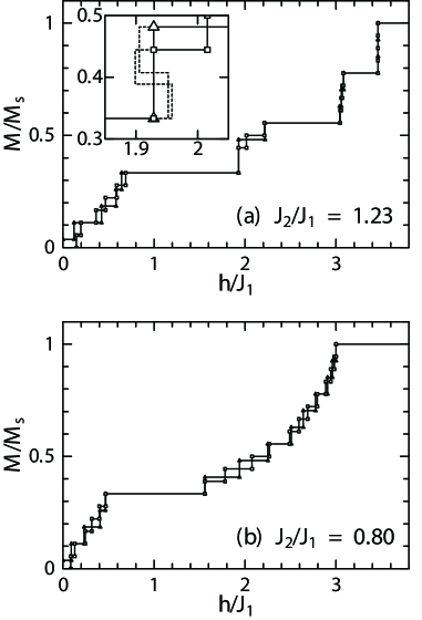
Figure 5: Magnetization process for the $S=1/2$ Heisenberg antiferromagnet on the $\sqrt{3}\times\sqrt{3}$ distorted kagome lattice. Panels (a) and (b) show the cases of $J_{2}/J_{1}$=1.23 and 0.80, respectively. Squares and triangles are the results for $N_{\rm s}=36$ and 27, respectively. The inset in (a) shows a zoomed-in view at the higher-field edge of the one-third height of the saturation, where the broken lines represent the results before the Maxwell construction is carried out.

The same spin-flop phenomenon is reported in the square-kagome lattice[33] and shuriken-bonded honeycomb lattice[32]. Figure 5 (a) shows the same behavior at $J_{2}/J_{1}=1.23$. However, the investigation reported in Ref. References focused on the case of $J_{2}/J_{1}>1$. To study the behavior at around the undistorted point $J_{2}/J_{1}=1$, the present study treats not only the case of $J_{2}/J_{1}>1$ but also the case of $J_{2}/J_{1}<1$.

We show the magnetization process for $J_{2}/J_{1}=0.80$ in Fig. 5 (b). One easily finds that several features are different between the cases of $J_{2}/J_{1}$=1.23 and 0.80. Contrary to the magnetization plateaux at $m=5/9$ and 7/9 observed in the case of $J_{2}/J_{1}$=1.23, the widths at these heights in the case of $J_{2}/J_{1}$=0.80 become markedly smaller, suggesting the disappearance of the plateaux. The magnetization jump between $m=7/9$ and the saturation is observed in the case of $J_{2}/J_{1}$=1.23 owing to the formation of explicit eigenstates with a spatially localized structure at hexagons on the kagome lattice. In the case of $J_{2}/J_{1}$=0.80, the jump also disappears. On the other hand, the behavior at $m=1/3$ is similar between the cases of $J_{2}/J_{1}$=1.23 and 0.80; the state of $m=1/3$ is realized in a wide region of external field, suggesting the existence of the magnetic plateau.

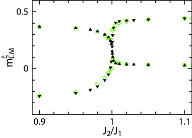
Figure 6: (Color) Dependence of the local magnetization on the ratio of interaction $J_{2}/J_{1}$. For $N_{\rm s}=27$, closed triangles and closed inversed triangles denote the results of $\xi=\alpha$ and $\beta$, respectively. For $N_{\rm s}=36$, green open squares and green open diamonds denote the results for $\xi=\alpha$ and $\beta$, respectively.

To examine whether the properties of the $m=1/3$ states for $J_{2}/J_{1}$=1.23 and 0.80 are the same or different, we evaluate the local magnetization defined as

$$m_{\rm LM}^{\xi}=\frac{1}{N_{\xi}}\sum_{j\in\xi}\langle S_{j}^{z}\rangle,$$ (13)

where $\xi$ takes $\alpha$ and $\beta$. Here, the symbol $\langle{\cal O}\rangle$ denotes the expectation value of the operator ${\cal O}$ with respect to the lowest-energy state within the subspace with a fixed $M$ of interest. Recall here that the case of interest in this paper is $M=M_{\rm s}/3$. Here $N_{\xi}$ denotes the number of $\xi$ sites; averaging over $\xi$ is carried out in the case when the ground-state level is degenerate. Note that, for $M$ with nondegenerate ground states, the results do not change regardless of the presence or absence of this average. Our results of $m_{\rm LM}^{\xi}$ are shown in Fig. 6. One clearly observes a large increase in $m_{\rm LM}^{\beta}$ and a large decrease in $m_{\rm LM}^{\alpha}$ at approximately $J_{2}/J_{1}=1$. In the region of $J_{2}/J_{1}>1$, an $\alpha$-site spin becomes almost vanishing, while a $\beta$-site spin becomes an up-spin. This spin state has already been discussed in Ref. References: the state is composed of a spin-singlet at two neighboring $\alpha$ spins and an up-spin at a $\beta$ site in each local triangle of the lattice. In the region of $J_{2}/J_{1}<1$, on the other hand, an $\alpha$-site spin becomes an up-spin while a $\beta$-site spin becomes a down-spin. This spin state is easily understood if one considers the case of $J_{2}/J_{1}=0$. In this limiting case, the Marshall-Lieb-Mattis theorem[34, 35] holds. Therefore, the ferrimagnetic state with the up-spin at the $\alpha$ site and the down-spin at the $\beta$ site is realized as the ground state with a spontaneous magnetization even in the absence of a magnetic field. The result in Fig. 6 suggests that, in the region of $J_{2}/J_{1}<1$ near $J_{2}/J_{1}=1$, the same ferrimagnetic state appears under some external field. It is an unresolved issue where the phase transition to such a Lieb-Mattis-type ferrimagnetic state as the ground state with a spontaneous magnetization occurs. A related problem was investigated in the spatially anisotropic kagome-lattice antiferromagnet in Refs. References and References, which pointed out the existence of the non-Lieb-Mattis phase in the intermediate region between the Lieb-Mattis-type ferrimagnetic phase and the nonmagnetic phase. Note here that this intermediate ferrimagnetic state is observed in various one-dimensional systems[38, 39, 40, 41]. It is also an unresolved issue whether such an intermediate phase is present or absent in the present distortion of the $\sqrt{3}\times\sqrt{3}$ type. The most important consequence is a marked change in $m_{\rm LM}^{\alpha}$ and $m_{\rm LM}^{\beta}$ at $J_{2}/J_{1}=1$, suggesting the occurrence of a quantum phase transition. In Refs. References and References, a similar observation about the local magnetization was reported in the $S=1/2$ Heisenberg antiferromagnet on the Cairo-pentagon lattice[44, 45]. One difference is that the boundary is independent of $N_{\rm s}$ and is $J_{2}/J_{1}=1$ for both $N_{\rm s}=27$ and 36. Unfortunately, it is difficult to conclude whether the transition is of the second or first order because the change in $m_{\rm LM}^{\xi}$ is continuous for $N_{\rm s}=36$, while it is discontinuous for $N_{\rm s}=27$ from examinations based on the numerical-diagonalization data.

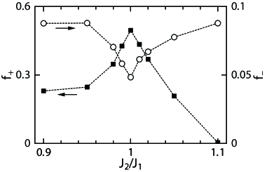
Figure 7: Dependences of $f_{+}(N_{\rm s})$ and $f_{-}(N_{\rm s})$ for $N_{\rm s}=36$ on the ratio of interaction $J_{2}/J_{1}$ around the undistorted point. Closed squares and open circles denote $f_{+}(N_{\rm s})$ and $f_{-}(N_{\rm s})$, respectively.

Finally, let us observe the change at approximately $J_{2}/J_{1}=1$ just outside $m=1/3$ in the magnetization process. To do so, we examine the dependences of $f_{+}(N_{\rm s})$ and $f_{-}(N_{\rm s})$ on the ratio $J_{2}/J_{1}$; the result for $N_{\rm s}=36$ is shown in Fig. 7. One easily observes different dependences on $J_{2}/J_{1}$ between the regions of $J_{2}/J_{1}>1$ and $J_{2}/J_{1}<1$. This difference appears regardless of $f_{+}(N_{\rm s})$ and $f_{-}(N_{\rm s})$. This result strongly suggests the existence of some boundary at $J_{2}/J_{1}=1$. One finds that the behavior of $f_{+}(N_{\rm s})$ at $J_{2}/J_{1}=1$ is maximum, while that of $f_{-}(N_{\rm s})$ at $J_{2}/J_{1}=1$ is minimum. Although the reason for this contrast is currently unresolved, the undistorted point is certainly a boundary.

4 Conclusions

We have studied the Heisenberg antiferromagnet on the kagome lattice without and with a distortion of the $\sqrt{3}\times\sqrt{3}$ type by the numerical-diagonalization method. We present a new result of the magnetization process for this undistorted model for a 42-site cluster for the first time. Our diagonalization results suggest that the critical exponents of the field dependence of the magnetization just outside of the one-third magnetization state are markedly different from the exponent $\delta=1$ for the typical magnetization plateau in a two-dimensional system. On the other hand, we do not obtain positive evidence of the vanishing width at the one-third magnetization state even if we take into account our new result of the 42-site cluster. Our results of the distorted model clearly indicate that the undistorted kagome point is a boundary between two regions: the ferrimagnetic state and the state with the nine-site structure including a hexagonal singlet and three up-spins. The change near the undistorted point as the transition point is very rapid. It is unclear whether the phase transition is continuous or discontinuous at the present stage. At such a transition point, the anomalous critical exponents are not so unnatural.

In Ref. References, the authors proposed that the one-third magnetization state is well described by the state with the nine-site structure including a hexagonal singlet and three up-spins. This picture of the state is in disagreement with the present consequence that the undistorted point is just a boundary. A possible reason for this discrepancy is that the deformation used in Ref. References plays an essential role as a perturbation added to the ideal kagome-lattice antiferromagnet and that the case that the calculation in Ref. References captures may, therefore, not be only the ideal kagome-lattice antiferromagnet but is a case that deviated slightly from the ideal point, which is the transition point. Even though the deviation is taken to be very small, a difficulty is possibly unavoidable in capturing the true behavior only on the transition point. The present study of the kagome-lattice antiferromagnet suggests that a method based on a deformation technique possibly reaches an incorrect conclusion concerning subtle behaviors near the transition point.

Another distortion introduced into the kagome lattice was studied from the viewpoint of continuously linking the kagome and triangular lattices[46, 47]. Concerning the $m=1/3$ state, Refs. References and References showed that the phase transition occurs between the kagome and triangular points and that the kagome point is close to but different from the transition point. Note here that this type of distortion was realized in an experimental study[48]; the direct comparison is difficult at the present time because the spin is larger than $S=1/2$. If an experimental realization of an $S=1/2$ system is successful, the comparison between the experiments and theoretical predictions would be useful for our deeper understanding of quantum spin systems. Studies of other types of distortion would also contribute to the progress of this field.

References

- [1] M. P. Shores, E. A. Nytko, B. M. Barlett, and D. G. Nocera, J. Am. Chem. Soc. 127, 13462 (2005).
- [2] P. Mendels and F. Bert, J. Phys. Soc. Jpn. 79, 011001 (2010).
- [3] H. Yoshida, Y. Okamoto, T. Tayama, T. Sakakibara, M. Tokunaga, A. Matsuo, Y. Narumi, K. Kindo, M. Yoshida, M. Takigawa, and Z. Hiroi, J. Phys. Soc. Jpn. 78, 043704 (2009).
- [4] M. Yoshida, M. Takigawa, H. Yoshida, Y. Okamoto, and Z. Hiroi, Phys. Phys. Lett. 103, 077207 (2009).
- [5] Y. Okamoto, H. Yoshida, and Z. Hiroi, J. Phys. Soc. Jpn. 78, 033701 (2009).
- [6] Y. Okamoto, M. Tokunaga, H. Yoshida, A. Matsuo, K. Kindo, and Z. Hiroi, Phys. Rev. B 83, 180407 (2011).
- [7] P. Lecheminant, B. Bernu, C. Lhuillier, L. Pierre, and P. Sindzingre, Phys. Rev. B 56, 2521 (1997).
- [8] C. Waldtmann, H.-U. Everts, B. Bernu, C. Lhuillier, P. Sindzingre, P. Lecheminant, and L. Pierre, Eur. Phys. J. B 2, 501 (1998).
- [9] K. Hida, J. Phys. Soc. Jpn. 70, 3673 (2001).
- [10] D. C. Cabra, M. D. Grynberg, P. C. W. Holdsworth, and P. Pujol, Phys. Rev. B 65, 094418 (2002).
- [11] J. Schulenburg, A. Honecker, J. Schnack, J. Richter, and H.-J. Schmidt, Phys. Rev. Lett. 88, 167207 (2002).
- [12] A. Honecker, J. Schulenburg, and J. Richter, J. Phys.: Condens. Matter 16, S749 (2004).
- [13] D. C. Cabra, M. D. Grynberg, P. C. W. Holdsworth, A. Honecker, P. Pujol, J. Richter, D. Schmalfß, and J. Schulenburg, Phys. Rev. B 71, 144420 (2005).
- [14] O. Cpas, C. M. Fong, P. W. Leung, and C. Lhuillier, Phys. Rev. B 78, 140405(R) (2008).
- [15] P. Sindzingre and C. Lhuillier, Europhys. Lett. 88, 27009 (2009).
- [16] H. Nakano and T. Sakai, J. Phys. Soc. Jpn. 79, 053707 (2010).
- [17] T. Sakai and H. Nakano, Phys. Rev. B 83, 100405(R) (2011).
- [18] H. Nakano and T. Sakai, J. Phys. Soc. Jpn. 80, 053704 (2011).
- [19] A. Honecker, D. C. Cabra, H.-U. Everts, P. Pujol, and F. Stauffer, Phys. Rev. B 84, 224410 (2011).
- [20] S. Capponi, O. Derzhko, A. Honecker, A. M. Luchli, and J. Richter, Phys. Rev. B 88, 144416 (2013).
- [21] H. C. Jiang, Z. Y. Weng, and D. N. Sheng, Phys. Rev. Lett. 101, 117203 (2008).
- [22] S. Yan, D. A. Huse, and S. R. White, Science 332, 1173 (2011).
- [23] S. Depenbrock, I. P. McCulloch, and U. Schollwock, Phys. Rev. Lett. 109, 067201 (2012).
- [24] S. Nishimoto, N. Shibata, and C. Hotta, Nat. Commun. 4, 2287 (2013).
- [25] C. Hotta and N. Shibata, Phys. Rev. B 86, 041108 (2012).
- [26] Note that there are some reports on partial-range magnetization processes with a large , for example, Ref. References.
- [27] H. Nakano and A. Terai, J. Phys. Soc. Jpn. 78, 014003 (2009).
- [28] H. Nakano, S. Todo, and T. Sakai, J. Phys. Soc. Jpn. 82, 043715 (2013).
- [29] M. Kohno and M. Takahashi, Phys. Rev. B 56, 3212 (1997).
- [30] T. Sakai and M. Takahashi, Phys. Rev. B 60, 7295 (1999).
- [31] T. Sakai and M. Takahashi, Phys. Rev. B 57, R8091 (1998).
- [32] H. Nakano, T. Sakai, and Y. Hasegawa, arXiv:1406.4964.
- [33] H. Nakano and T. Sakai, J. Phys. Soc. Jpn. 82, 083709 (2013).
- [34] W. Marshall, Proc. R. Soc. London, Ser. A 232, 48 (1955).
- [35] E. Lieb and D. Mattis, J. Math. Phys. (N.Y.) 3, 749 (1962).
- [36] H. Nakano, T. Shimokawa, and T. Sakai, J. Phys. Soc. Jpn. 80, 033709 (2011).
- [37] T. Shimokawa and H. Nakano, J. Phys. Soc. Jpn. 81, 084710 (2012).
- [38] K. Hida, J. Phys.: Condens. Matter 19, 145225 (2007).
- [39] K. Hida and K. Takano, Phys. Rev. B 78, 064407 (2008).
- [40] T. Shimokawa and H. Nakano: J. Phys. Soc. Jpn. 80, (2011) 043703.
- [41] T. Shimokawa and H. Nakano: J. Phys. Soc. Jpn. 80, (2011) 125003.
- [42] H. Nakano, M. Isoda, and T. Sakai, J. Phys. Soc. Jpn. 83, 053702 (2014).
- [43] M. Isoda, H. Nakano, and T. Sakai, to be published in J. Phys. Soc. Jpn.
- [44] E. Ressouche, V. Simonet, B. Canals, M. Gospodinov, and V. Skumryev, Phys. Rev. Lett. 103, 267204 (2009).
- [45] I. Rousochatzakis, A. M. Luchli, and R. Moessner, Phys. Rev. B 85, 104415 (2012).
- [46] T. Sakai and H. Nakano, Phys. Status Solidi B 250, 579 (2013).
- [47] H. Nakano and T. Sakai, JPS Conf. Proc. 3, 014003 (2014).
- [48] H. Ishikawa, T. Okubo, Y. Okamoto, and Z. Hiroi, J. Phys. Soc. Jpn. 83, 043703 (2014).