Abstract

Applications of first passage times in stochastic processes arise across a wide range of length and time scales in biological settings. After an initial technical overview, we survey representative applications and their corresponding models. Within models that are effectively Markovian, we discuss canonical examples of first passage problems spanning applications to molecular dissociation and self-assembly, molecular search, transcription and translation, neuronal spiking, cellular mutation and disease, and organismic evolution and population dynamics. In this last application, a simple model for stem-cell aging is presented and some results derived. Various approximation methods and the physical and mathematical subtleties that arise in the chosen applications are also discussed.

Chapter 0 First Passage Problems in Biology

1 Introduction & Mathematical Preliminaries

Although mainly studied in physical systems, first passage problems [1] arise in many biological contexts, including biomolecular kinetics, cellular function, and population dynamics. First passage problems can be most simply described as finding the distribution of times according to which a random process first exceeds a prescribed threshold or reaches a specified configuration, as described in Fig. 1. While expectations of moments of the random variable are often qualitatively captured by using straightforward approximation methods, other observable quantities such as first passage times may not be, and stochastic approaches must be used.

The probability distribution $P(X,t)$ of a stochastic process $X(t)$ may obey a discrete master equation or a Fokker-Planck or Smoluchowski equation for continuous variables. Other approaches such as the direct analysis of stochastic differential equations (SDEs) for the random variable $X(t)$ or analysis of the branching process [2, 3] describing the evolution of the probability generating function is also often employed. If the system does not harbour long-lived metastable configurations, simple mean-field or closure methods that approximate correlations can be used to analytically find expected trajectories $\langle X(t)\rangle=\int XP(X,t)\mbox{d}X$ that are often in qualitative agreement with exact results or trajectories derived from approximate, deterministic models.

Figure 1: Trajectories of a random variable $X(t)$ illustrating typical first passage problems. (a) The deterministic or expected trajectory $\langle X(t)\rangle$ (solid black curve) crosses the specified threshold $X^{*}=0.2$ at a specific time $T\approx 1.6$; however, when fluctuations are explicitly included, the random variable $X(t)$ can cross $X=0.2$ at different times $T\approx 1.45$ and $T\approx 1.7$, as shown by the red and blue trajectories, respectively. (b) The distribution of first passage times to $X=0.2$. (c) Trajectories corresponding to a birth-death process with carrying-capacity (see Eq. 44 in Section 6). In the deterministic model, $X=10$ (the carrying-capacity in this example) is a stable fixed point while $X=0$ is an unstable one. With an initial condition $X(0)>0$, the deterministic model never becomes extinct $(X^{*}=0)$, but in a stochastic model a random (possibly very rare) fluctuation can extinguish the system. The distribution of first extinction times is schematically shown in (d).

For example, consider the trajectories depicted in Fig. 1. Some deterministic trajectories $\langle X(t)\rangle$ cross a threshold value ($X^{*}=0.2$ in Fig. 1(a)) at a unique time $T$, which then can be used as a qualitatively good estimate of the first passage time for the full stochastic process. However, in other cases, the deterministic trajectory may never cross a predefined “absorbing” threshold so that $T=\infty$. This is illustrated in Fig. 1(c) where $X(t)$ never reaches the threshold value $X^{*}=0$. However, in a stochastic model, fluctuations can bring $X(t)$ to the threshold $X^{*}=0$ in finite time. For such cases, there is a clear divergence between the exit times predicted from a deterministic model ($T=\infty$) and that predicted from a stochastic one ($T<\infty$).

To be more concrete, consider a discrete Markov process for a system of $N$ states that can be described by the “forward” master equation

$${\partial P_{ki}\over\partial t}=M_{kj}P_{ji},$$ (1)

where $P_{ki}$ is the $N\times N$ matrix of probabilities that the system is in configuration $k$ at time $t$, given that the system started in state $i$ at $t=0$. The $N\times N$ transition matrix composed of transition rates that take state $j$ to state $k$ is defined by $M_{kj}$. Note that $(k,j)$ indexes all accessible configurations, including absorbing ones ${\cal A}$ from which probability density cannot re-emerge. Transition rates out of configurations ${\cal A}$ are defined to be zero while global probability conservation requires $\sum_{k=1}^{N}M_{kj}=0$. As the dynamics evolve, the flow of probability entering absorbing states ${\cal A}$ cannot exit. Eventually, the survival probability defined as $S_{i}(t)\equiv\sum_{k\notin{\cal A}}P_{ki}(t)$ will vanish as $t\to\infty$. The survival probability $S_{i}(t)$ defines the probability that the system has not reached any absorbing configuration up to time $t$, given that it started in configuration $i$ at $t=0$.

Since the first passage time distribution can be derived from $S_{i}(t)$, it is convenient to consider the adjoint equation that is also obeyed by $P_{ki}(t)$ only if the transition matrix $M_{kj}$ is time-independent:

$${\partial P_{ki}\over\partial t}=P_{kj}M_{ji}.$$ (2)

This “backward” equation does not operate on the final configurations $k$ so one can perform the sum $\sum_{k\notin{\cal A}}$ to find an equation for the survival probability

$${\partial S_{i}(t)\over\partial t}=S_{j}(t)M_{ji},$$ (3)

along with the initial condition $S_{k}(t=0)=1$ for $k\notin{\cal A}$ and “boundary condition” $S_{k}(t)=0$ for $k\in{\cal A}$.

A physical interpretation of Eq. 3 can be easily obtained by considering the lifetime distribution function which is a sum over the absorbed states: $F_{i}(t)\equiv\sum_{k\in{\cal A}}P_{ki}(t)=1-S_{i}(t)$. We can now identify the rate of change of $F_{i}$ as the probability flux into the absorbing state ${\cal A}$, so that $\partial_{t}F_{i}\equiv J^{\cal A}_{i}(t)$. Using $F_{j}\equiv 1-S_{j}$, we can rewrite Eq. 3 as

$${\partial S_{i}(t)\over\partial t}=S_{j}(t)M_{ji}=-J_{i}^{\cal A}(t).$$ (4)

The latter is also a statement that the probability of survival against entering absorbing configurations decreases in time according to the probability flux into the absorbing states.

From the lifetime distribution $F_{i}(t)$, one can find the probability that the system reached any absorbing configuration between time $t$ and $t+\mbox{d}t$ as $F_{i}(t+\mbox{d}t)-F_{i}(t)=S_{i}(t)-S_{i}(t+\mbox{d}t)$. Hence, the first passage time distribution $w_{i}(t)$ can be found from

$$w_{i}(t)\mbox{d}t\equiv{\partial F_{i}(t)\over\partial t}\mbox{d}t=-{\partial S_{i}(t)\over\partial t}\mbox{d}t,$$ (5)

allowing calculation of all moments $n$ of the first passage time

$$\langle T_{i}^{n}\rangle=\int_{0}^{\infty}w_{i}(t)t^{n}\mbox{d}t.$$ (6)

Upon using integration by parts for $n=1$, the mean first passage time is simply $\langle T_{i}\rangle=\int_{0}^{\infty}S_{i}(t)\mbox{d}t$. Integrating Eq. 4 directly, we find an explicit equation for the moments of the first passage time into an absorbing state

$$\langle T_{j}^{n}\rangle M_{ji}=-n\langle T^{n-1}_{i}\rangle,$$ (7)

where $\langle T_{j}^{0}\rangle\equiv 1$. Equations 6 and 7 have been used to study moments of first exit times for a random walker to hit either one or two ends of a discrete one-dimensional lattice [4, 5].

A commonly used approximation to Eq. 4 (see Sections 2 and 4) is to assume

$${\partial S_{i}(t)\over\partial t}\approx-J_{i}^{\cal A}(t)S_{i}(t),$$ (8)

which is motivated by a mass-action argument of the decay of probability of being in the initial surviving state $i$. Here, $J_{i}^{\cal A}(t)$ is the probability current from state $i$ to ${\cal A}$. However, the RHS of the exact relationship in Eq. 4 contains the transition matrix $M_{ji}$ which mixes states $i$ with $j$. Since the approximation in Eq. 8 does not resolve the different surviving states, Eq. 8 is exact only when there is a single surviving state $i$ that directly transitions into ${\cal A}$ without any intermediate states. Another limit where Eq. 8 is accurate is if the system mixes quickly among all surviving states well before being absorbed. In this case, the single surviving state $i$ is a lumped average over all the microscopic states $j$, and first passage can be thought of as slow degradation of a quasi-steady-state configuration. Equation 8 and the associated assumptions have been widely used in practice, particularly to describe bond rupturing in dynamic force spectroscopy of biomolecules (see Section 2).

Another common representation of stochastic processes that is useful for modeling biophysical systems is based on continuous variables. This “Lagrangian” representation is particularly suitable for tracking stochastically-moving, identifiable particles. Starting from Eq. 1, a continuum formulation can be heuristically developed by assuming that each configuration is connected to only a few others. In this case, indices can be chosen such that the transition matrix is banded. For example, a particle at position $i$ on a one-dimensional lattice is allowed to jump only to neighboring positions $i\pm 1$ with probability proportional to an infinitesimal increment of time. If the indices label lattice site positions, the transition matrix will be tridiagonal. Furthermore, if the transition rates vary slowly from site to site, and the system size $N$ is large, we can take a continuum limit where the position of a particle $y=i/N$ and the tridiagonal transition matrix represents a stencil of a differentiation operator.

Upon defining $P(\{{\bf y}_{j}\},t|\{{\bf x}_{j}\},0)$ as the probability that all particles $j$ are located between ${\bf y}_{j}$ and ${\bf y}_{j}+\mbox{d}{\bf y}_{j}$ at time $t$ given that they were at positions $\{{\bf x}_{j}\}$ at $t=0$, one can Taylor-expand a discrete master equation in a “diffusion approximation” to find the governing Fokker-Planck or Smoluchowski equation

$$\begin{array}[]{rl}\displaystyle{\partial P(\{{\bf y}_{j}\},t|\{{\bf x}_{j}\},0)\over\partial t}&=-\sum_{k=1}^{N}\nabla_{k}\cdot({\bf V}_{k}P)+\sum_{k=1}^{N}\nabla_{k}^{2}(D(\{{\bf y}_{k}\})P)\\[13.0pt] &\displaystyle\equiv{\cal L}P(\{{\bf y}_{j}\},t|\{{\bf x}_{j}\},0),\end{array}$$

where here, $N$ is the total number of particles, ${\bf V}_{k}$ is the drift velocity of the $k^{\rm th}$ particle, and the gradient $\nabla_{k}$ is taken with respect to the coordinates of the $k^{\rm th}$ particle. The density $P(\{{\bf y}_{j}\},t|\{{\bf x}_{j}\},0)$ also obeys the Backward Kolmogorov Equation (BKE) which is simply

$$\partial_{t}P(\{{\bf y}_{j}\},t|\{{\bf x}_{j}\},0)={\cal L}^{\dagger}P(\{{\bf y}_{j}\},t|\{{\bf x}_{j}\},0),$$ (9)

where ${\cal L}^{\dagger}=\sum_{k}^{N}{\bf V}_{k}\cdot\nabla_{k}+\sum_{k=1}^{N}D(\{{\bf x}_{j}\})\nabla_{k}^{2}$ is the operator adjoint of ${\cal L}$. Since ${\cal L}^{\dagger}$ operates on the initial positions ${\bf x}_{j}$, Eq. 9 can be integrated over coordinates ${\bf y}_{j}$ within the domain, excluding the absorbing surfaces. The resulting equation for the survival probability analogous to Eq. 4 is $\partial_{t}S(\{{\bf x}_{j}\};t)={\cal L}^{\dagger}S(\{x_{j}\};t)$, with $S(\{x_{j}\};t=0)=1$ for all ${\bf x}_{j}\neq\partial\Omega_{{\cal A}}$, and $S(\forall{\bf x}_{j}=\partial\Omega_{\cal A};t)=0$. From this survival probability, all moments of the first times any particle hits an absorbing boundary $\partial\Omega_{{\cal A}}$ can be derived. Namely, in analogy with Eq. 7, the mean hitting time obeys

$${\cal L}^{\dagger}\langle T^{n}(\{x_{j}\})\rangle=-n\langle T^{n-1}(\{x_{j}\})\rangle.$$ (10)

Both the discrete and continuum stochastic formulations are commonly applied to physical systems; however, care should be exercised in using a continuum description as an approximation for a discrete system where first passage times are sought. Although the continuum diffusion approximation may be accurate in describing probability densities of large discrete systems, it often provides a poor approximation to first passage times of discrete processes. Indeed, using a birth-death process with carrying-capacity (see Section 6), Doering, Sagsyan, and Sander [6] show that the effective potential of a discrete system and its corresponding continuum diffusion approximation differ, leading to different mean first population extinction times. The discrepancy is small only when the convective term in the Fokker-Planck equation is small across all relevant population levels. Thus, depending on the application, continuum diffusion approximations and their numerical discretization should be applied judiciously when first passage times are being analyzed.

The first passage problems defined above assume that one is interested in the distribution of times of the systems arriving at any absorbing configuration. However, there may well be states which are physically absorbing (into which probability flux enters irreversibly) but that are not relevant to the biological process. For example, one may be interested in the times it takes for a diffusing protein to first reach a certain target site (see Section 4 below), but the protein may degrade before reaching it. Since decay is irreversible, the system reaches an “unintended” absorbing state through degradation of the protein. If one defines ${\cal A}$ to be only the biologically-relevant absorbing configurations, the corresponding survival probability $S_{i}(t)$ does not vanish in the $t\to\infty$ limit because there are other “irrelevant” absorbing states that absorb some of the probability. In other words, if there are other physical absorbing states competing for probability, the integrated probability flux $J_{i}^{\cal A}(t)$ into the relevant absorbing states ${\cal A}$ obeys $\int_{0}^{\infty}J^{\cal A}_{i}(t)\mbox{d}t<1$. Also note that since $S_{i}(t\to\infty)>0$, the mean first passage time $\langle T_{i}\rangle=\int_{0}^{\infty}S_{i}(t)\mbox{d}t=\infty$. All moments also diverge. Provided a measurable fraction of trajectories reach the irrelevant absorbing state, the mean time to arrive at the relevant absorbing state diverges because these “wasted” trajectories will never reach the relevant states.

A more appropriate measure in cases with “interfering” absorbing states is the distribution of first arrival times conditioned on arriving at the relevant absorbing configurations ${\cal A}$. In other words, we restrict ourselves to the arrival time statistics of only those trajectories that are not absorbed by the irrelevant states. The conditioning is a simple statement of Bayes rule: $J^{\cal A}_{i}(t)=J_{i}(t|{\cal A})\times\mbox{Prob(exiting through}\,{\cal A})$, where $J^{\cal A}_{i}(t)$ is the overall probability flux from $i$ into ${\cal A}$, and $J_{i}(t|{\cal A})$ is the probability flux of annihilation counting those trajectories that annihilate through the relevant absorbing states ${\cal A}$. Since the probability of exiting through ${\cal A}$ is $\int_{0}^{\infty}J_{i}^{\cal A}(t)\mbox{d}t$, the conditional first passage time distribution is

$$J_{i}(t|{\cal A})\mbox{d}t\equiv w_{i}(t|{\cal A})\mbox{d}t={J_{i}^{\cal A}(t)\mbox{d}t\over\int_{0}^{\infty}J_{i}^{\cal A}(t^{\prime})\mbox{d}t^{\prime}}.$$ (11)

Analogous expressions for the continuum representation (Eq. 1) can be found provided a suitable continuum expression for the probability flux is used. As a simple example, consider a single Brownian particle with diffusivity $D$ in one dimension with absorbing boundaries at $x=\pm 1$. The probability flux through the ends are

$$\mp D{\partial P(y,t|x,0)\over\partial y}\bigg{|}_{y=\pm 1}\equiv J_{x}(t|\pm 1).$$ (12)

The first passage time distributions sampled over only those trajectories that exit, say, $y=+1$ is thus

$$w_{x}(t|+1)\mbox{d}t={J_{x}(t|+1)\mbox{d}t\over\int_{0}^{\infty}J_{x}(t^{\prime}|+1)\mbox{d}t^{\prime}},$$ (13)

which can be explicitly calculated given the solution to the diffusion equation (Eq. 1) for $P(y,t|x,0)$.

The mathematical approaches presented above, along with many extensions, have been used to model a diverse set of first passage problems arising in biological systems. In the following sections, we survey some illustrative examples of such first passage problems that span length scales ranging from the molecular, to the cellular, to that of populations.

2 Molecular rupture

The times over which molecules dissociate play an important role in chemical biology. For example, ligand-receptor complexes have finite lifetimes that are important determinants of whether signalling is initiated. Cell-substrate and cell-cell adhesion are also mediated by molecules such as glycoproteins [7], and knowing the “strength” of these macromolecular bonds can reveal insight into the biological function of macromolecules.

For a simple single-barrier free energy profile, one simple approximation is to assume a quadratic energy profile and compute the first passage time distribution to a particular displacement, reducing the calculation to that of finding the first crossing time of an over-damped Ornstein-Ulhenbeck process [8, 9]. Another more refined approximation concatenates two harmonic potentials (one of positive curvature, one of negative curvature) together to form an approximate potential. Upon using steepest descents, a simple expression for the mean bond rupturing time starting from the energetic minimum $\xi_{0}$ can be found in the high barrier (rare crossing) limit:

$$\langle T(\xi_{0})\rangle\approx{e^{-(U(\xi^{*})-U(\xi_{0}))}\over 2\pi|\kappa_{0}\kappa_{*}|}.$$ (14)

Here, $\kappa_{0}$ and $\kappa_{*}$ are the curvatures of the potential at the local minimum and at the top of the barrier, respectively. Since the barrier is high, and dissociation is a rare event, the distribution of rupturing times can be well-approximated by a single exponential with a dissociation rate $k_{\rm d}\equiv 1/\langle T\rangle$. In addition to the barrier height, Eq. 14 encodes the shape of the bond potential through the curvatures $\kappa_{0}$ and $\kappa^{*}$. However, typical bonds are sufficiently strong such that their rupture times are too large to be experimentally accessible. Therefore, bonds are typically pulled by external forces in “dynamic force spectroscopy” (DFS) experiments.

Ideally, in a DFS experiment, the applied force on the bond that is typically linearly ramped up (in time) until the bond ruptures, and some properties of the bond trajectories or forces sampled [10, 11]. From these data, one may seek to reconstruct properties of the underlying pre-pulled potential. Therefore, under an assumption of no rebinding, analysis of DFS can be reduced to a first passage problem with a time-dependent potential. Nearly all approaches to this problem have included the pulling into a time-dependent free energy barrier $U(\xi,t)$, giving rise to a time-dependent dissociation rate $k_{\rm d}(t)$, which is then used in the mean-field equation (Eq. 8) for the bond survival probability $\dot{S}(t)\approx-k_{\rm d}(t)S(t)$. As it stands, this rate equation does not provide information about the bond other than the effective barrier height. In order to model finer effects of the bond energy profiles, shape properties need to be incorporated into the analysis. The simplest way to do this is to model how $k_{\rm d}(t)$ depends on the shape of the bond energy, while still retaining the mean-field assumption (Eq. 8) for the survival probability [11].

One simple approach is to assume the bond potential contains a barrier at bond coordinate $\xi^{*}$, beyond which the bond is irreversibly dissociated. To approximate the distribution of times for a bond to spontaneously rupture, one calculates the time it takes for a random walker to reach the “absorbing boundary” $\xi^{*}$, given that it started from an initial position $\xi_{0}$. The standard calculation proceeds by solving the Fokker-Planck equation for the probability density $P(\xi,t|\xi_{0},0)$ and constructing the corresponding survival probability $S(\xi_{0};t)=\int_{0}^{\xi_{*}}P(\xi,t|\xi_{0},0)\mbox{d}\xi$, or, alternatively, directly solving the Backward Kolmogorov Equation for $S(\xi_{0};t)$. The probability density, survival probability, and rupture time distribution are all easily solved numerically. In the over-damped limit of diffusive dynamics, the mean bond rupturing time $\langle T\rangle\equiv\int_{0}^{\infty}S(\xi_{0};t)\mbox{d}t$ can be found in exact closed form for any general free energy profile $U(\xi)$ [12].

The simplest way to incorporate a time-varying applied force problem in the one-dimensional continuum limit is to define an auxiliary time variable $\tau$ such that $\partial_{t}\tau=1$. In the backward equation corresponding to Eq. 10, $\tau$ is an independent variable [13]

$$\left({\partial\over\partial\tau}+F(\tau){\partial\over\partial\xi}+{\cal L}^{\dagger}\right)\langle T(\xi,\tau)\rangle=-1,$$ (15)

where $\xi$ is the initial starting coordinate of the bond and $F(\tau)=\gamma\tau$ describes a pulling force that is increased linearly with rate $\gamma$. With suitable boundary conditions $\langle T(\xi_{*},\tau)\rangle=\langle T(\xi,\infty)\rangle=0$, one can find the expected rupture time $\langle T(\xi,0)\rangle$ numerically.

Two analytical approximations can be made by assuming the pulling force $F$ is fixed. In this case, the solution to $\left(F\partial_{\xi}+{\cal L}^{\dagger}\right)\langle T(\xi,F)\rangle=-1$ is [13]

$$\langle T(\xi,F)\rangle=Q[\exp\left(-U(\xi)+F\xi)\right],$$ (16)

where $Q[...]$ is a complicated, but explicit integral functional [13]. In a first approximation Shillcock and Seifert [13] assumed that the typical rupturing force is determined self-consistently from $F^{*}\approx\gamma\langle T(\xi,F^{*})\rangle$.

A self-consistent approach to estimate the rupture force distribution is to solve the mean-field equation $\dot{S}(t;\xi_{0})=-k_{\rm d}(t)S(t;\xi_{0})$ and use Eq. 5 to find

$$w(\xi,t)\mbox{d}t=k_{\rm d}(\xi,t)\exp\left[-\int_{0}^{t}k_{\rm d}(\xi,t^{\prime})\mbox{d}t^{\prime}\right]\mbox{d}t,$$ (17)

where $k_{\rm d}(\xi,t)$ is the time-dependent rate of dissociation. Upon using $F(t)=\gamma t$ to convert this distribution to a rupture force distribution yields

$$\begin{array}[]{rl}w(\xi,F^{*})\mbox{d}F^{*}&\displaystyle={1\over\gamma}k_{\rm d}(\xi,F^{*})\exp\left[-{1\over\gamma}\int_{0}^{F^{*}}k_{\rm d}(\xi,F)\mbox{d}F\right]\mbox{d}F^{*}\\[13.0pt] &\displaystyle={1\over\gamma}k_{\rm d}(\xi,F^{*})\exp\left[-{1\over\gamma}\int_{0}^{F^{*}}{\mbox{d}F\over Q[\exp(-U(\xi)+F\xi)]}\right]\mbox{d}F^{*},\end{array}$$ (18)

where for the last equality, $k_{\rm d}(\xi,F)\approx 1/\langle T(\xi,F)\rangle$ and Eq. 16 were used. These and other mean-field approaches using Eq. 8 typically lead to a most probable rupture force $F^{*}$ that is proportional to $\ln\gamma$, with proportionality factors related to the spatial width and energetic depth of the underlying bond. Therefore, the rupture force distribution measured as a function of loading rate has been widely used as a quick measure of bond strength.

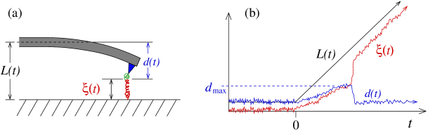
Figure 2: Schematic of an AFM-controlled bond-rupturing experiment. The AFM is lifted from the rigid substrate with prescribed displacement $L(t)$. The deflection $d(t)$ and the bond coordinate $\xi(t)$ sum to the total AFM displacement: $L(t)=d(t)+\xi(t)$. The deflection $d(t)$ is a measure of the bond-separating force through the relation $F(t)=k_{\rm s}d(t)$, where $k_{\rm s}$ is the known spring constant of the AFM cantilever.

While mathematically well-defined, the analyses above neglects a physical constraint encountered in bond pulling experiments. As noted by Qian and others [14, 15, 16], the mechanics of pulling a bond required the introduction of a mechanical spring force, whether manifested through an atomic force microscope (AFM) tip, an optical trap, or a pulled magnetic bead. If these devices are pulled with constant velocity $V$, the actual pulling potential is of the form $k_{\rm s}(\xi-Vt)^{2}/2$, where $k_{\rm s}$ is the spring constant of the AFM cantilever. The experimental setup depicted in Fig. 2 shows how the pulling force, including an estimate of the maximum force, can be measured through the deflection $d(t)$ of the cantilever.

This and related approximations are used in combination with specific bond energy profiles by many authors to derive expressions for rupture force distributions[17, 18, 19, 20, 21, 22, 23, 24]. For example, Dudko et al.[18] treat the ensemble where the pulling velocity $V$ is specified. They use a mean-field approximation for the bond survival probability (described in more detail in Section 4) and assume that the total potential is being shifted at a constant velocity $V$. For rather general potentials, they find a mean rupture force $\langle F^{*}\rangle\sim(\ln V)^{2/3}$, as well as an expression for the rupture force distribution. These results, however, rely on the use of a soft (small $k_{\rm s}$) pulling device. As shown in Fig. 3, a stiff puller (large $k_{\rm s}$) results in a single-well effective potential and a distinct rupture event is precluded [14, 15, 16]. In this case, it is not fruitful to analyze the problem within a first passage time framework, and a more careful analysis of the force distribution measured during the entire pulling protocol should be used.

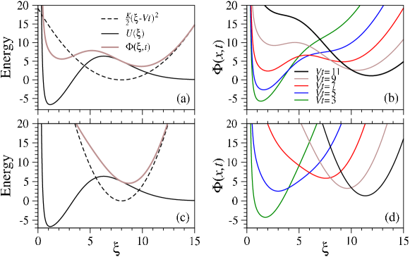
Figure 3: (a) Schematics of free energies as a function of an effective, one-dimensional bond coordinate $\xi$. The intrinsic molecular potential (black), harmonic potential of the pulling device (dashed), and the total potential (brown) are shown. (b) Only if the device potential is soft does the total potential $\Phi(\xi,t)$ form a barrier as the device is pulled. (c) If the pulling device is stiff, then only a single translating minimum arises, (d). Therefore, only for pulling devices with soft springs does a rupture event and corresponding rupture force qualitatively arise.

In general, the problem, as with many inverse problems is ill-posed [25]. The reconstruction of a potential from a single rupture time (or rupture force) distribution starting from a single bond coordinate is not unique [25], however, additional experiments (such as multiple loading forces and multiple starting bond positions) can give rise to multiple rupture time distributions that allow for reconstruction of potentials defined by many more parameters [26]. The extension of these inverse problems to those using rupture force distributions derived from different force loading rates could provide insight into the reconstruction of potentials more complex than simple harmonic, Lennard-Jones, or Morse type potentials.

3 Nucleation and self-assembly

A process complementary to dissociation is self-assembly, which also arises in many biological contexts. The polymerization of actin filaments [27, 28, 29, 30, 31] and amyloid fibrils [32], the assembly of virus capsids [33, 34, 35] and of antimicrobial peptides into transmembrane pores [36, 37], the assembly of ligands and receptors [38, 39], and the self-assembly of clathrin-coated pits [40, 41, 42] are all important processes at the cellular level that can be cast as self-assembly problems. Generally, in biological settings, there exists a maximum cluster size which signals the completion of the assembly process. For example, virus capsids, clathrin coated pits, and antimicrobial peptide pores typically consist of $N\sim 100-1000,N\sim 10-20$, and $N\sim 5-8$ molecular subunits, respectively. Furthermore, in confined spaces such as cellular compartments, the total mass is a conserved quantity. Figure 4 depicts a homogeneous nucleation process where monomers spontaneously bind and detach to clusters one at a time.

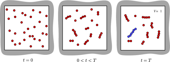
Figure 4: Homogeneous nucleation and growth in the slow detachment $(q\to 0^{+}$) limit in a closed unit volume initiated with $M=30$ monomers. If the constant monomer detachment rate $q$ is small, monomers will be nearly exhausted in the long time limit. In this example, we assume that $N=6$ is the maximum cluster size and that the first maximum cluster is formed at time $T$ (depicted in blue).

The classical description of self-assembly or homogeneous nucleation is a set of mass-action equations (such as the Becker-Döring equations) describing the concentration $c_{k}(t)$ of clusters of each size $k$ at time $t$:

$$\begin{array}[]{rl}\dot{c}_{1}(t)&=-pc_{1}^{2}-pc_{1}\sum_{j=2}^{N-1}c_{j}+2qc_{2}+q\sum_{j=3}^{N}c_{j}\\[13.0pt] \dot{c}_{2}(t)&=-pc_{1}c_{2}+{p\over 2}c_{1}^{2}-qc_{2}+qc_{3}\\[13.0pt] \dot{c}_{k}(t)&=-pc_{1}c_{k}+c_{1}c_{k-1}-qc_{k}+qc_{k+1}\\[13.0pt] \dot{c}_{N}(t)&=pc_{1}c_{N-1}-qc_{N},\end{array}$$ (19)

where for simplicity, we have assumed cluster size-independent attachment and detachment rates $p$ and $q$, respectively. These equations can readily be integrated to provide a mean-field approximation to the numbers of clusters of each possible size $k$ [43].

Given a total number of monomers $M$ one may be interested in the time it takes for the system to first assemble a complete cluster of size $N$. To address such a first passage problem, a stochastic model for the homogeneous nucleation process must be developed. Consider an $N$-dimensional probability density $P(n_{1},n_{2},\ldots,n_{N};t)$ for the system exhibiting at time $t$, $n_{1}$ free monomers, $n_{2}$ dimers, $n_{3}$ trimers…and $n_{N}$ completed clusters. The forward master equation obeyed by $P(n_{1},n_{2},\ldots,n_{N};t)$ is [43]:

$$\dot{P}(\{n\};t) = -\Lambda(\{n\})P(\{n\};t)+{1\over 2}(n_{1}+2)(n_{1}+1)W^{+}_{1}W^{+}_{1}W^{-}_{2}P(\{n\};t)$$

$$\displaystyle+\sum_{i=2}^{N-1}(n_{1}+1)(n_{i}+1)W^{+}_{1}W^{+}_{i}W^{-}_{i+1}P(\{n\};t)$$

$$\displaystyle+q(n_{2}+1)W^{+}_{2}W^{-}_{1}W^{-}_{1}P(\{n\};t)$$

$$\displaystyle+q\sum_{i=3}^{N}(n_{i}+1)W^{-}_{1}W^{-}_{i-1}W^{+}_{i}P(\{n\};t),$$ (20)

where we have rescaled time to $p^{-1}$. Here, $P(\{n\},t)=0$ if any $n_{i}<0$, $\Lambda(\{n\})={1\over 2}n_{1}(n_{1}-1)+\sum_{i=2}^{N-1}\!n_{1}n_{i}+q\sum_{i=2}^{N}n_{i}$ is total rate out of configuration $\{n\}$, and $W^{\pm}_{j}$ are the unit raising/lowering operators on the number of clusters of size $j$. For example,

$$\begin{array}[]{l}W^{+}_{1}W^{+}_{i}W^{-}_{i+1}P(\{n\};t)\equiv P(n_{1}+1,\ldots,n_{i}+1,n_{i+1}-1,\ldots;t).\end{array}$$ (21)

The process associated with this master equation has been analyzed using Kinetic Monte-Carlo simulations as well as asymptotic approximations for the mean cluster numbers in limits of small and large $q$ [43, 44].

The first passage problem is to determine the distribution of times for complete assembly of the largest cluster, $n_{N}=0\Rightarrow n_{N}=1$. For the purpose of illustration, consider a small system with $M=7$ or $8$, and $N=3$. Since state-space is small, we can visualize all possible configurations as shown in Fig. 5. The first passage time to a maximum cluster, starting from the all-monomer state ($P(\{n_{i}\};t=0)=\delta_{n_{1},M}\prod_{i=2}^{N}\delta_{n_{i},0}$) is the time the system takes to reach any of the states highlighted in blue, to the right of the red line.

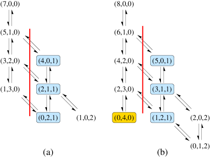
Figure 5: Allowed transitions in stochastic self-assembly starting from an all-monomer initial condition. In this simple example, the maximum cluster size $N=3$. (a) Allowed transitions for a system with $M=7$. Since we are interested in the first maximum cluster assembly time, states with $n_{3}=1$ constitute absorbing states. The process is stopped once the system crosses the vertical red line. (b) Allowable transitions when $M=8$. Note that if monomer detachment is prohibited ($q=0$), the configuration $(0,4,0)$ (yellow) is a trapped state. Since a finite number of trajectories will arrive at this trapped state and never reach a state where $n_{3}=1$, the mean first assembly time $T_{3}(8,0,0)\to\infty$ when $q=0$.

In the strong binding limit, when $0<q\ll 1$ and for $M$ even, one can find the dominant pathways to a largest cluster and surmise the leading order behavior $\langle T(q\ll 1)\rangle\sim 1/q$, with a prefactor that depends nontrivially on $M$ and $N$ [44]. This diverging assembly time arises from trapped states as highlighted in yellow in Fig. 5(b). As $q$ is increased, the likelihood of more paths coming out of the trapped states is higher, thereby decreasing the expected time to cluster completion. Only for the special case of $N=3$ and $M$ odd, where no such traps exist, is $\langle T(q)\rangle$ a nondivergent ratio of polynomials in $q$, as illustrated in Fig. 6(a).

In the weak binding, $q\gg 1$, maximum cluster formation is a rare event and $\langle T(q\gg 1)\rangle\sim q^{N-2}$. Because of these asymptotic relations, we expect at least a single minimum in the mean first assembly time as a function of detachment rate $q$ [44].

Figure 6: Mean first assembly times for $M=7$ and $N=3$ in panel (a) and $M=8$ and $N=3$ in panel (b). The notation $T_{N}(M,0,0)$ denotes the mean first maximum cluster (of size $N$) assembly time $\langle T\rangle$ starting from an initial condition of $M$ monomers. Exact results are plotted as black solid lines, while red circles are obtained by averaging over $10^{5}$ KMC simulation trajectories. The dashed blue lines show the $q\to 0$ and $q\to\infty$ asymptotic approximations.

Figure 6 shows $\langle T(q)\rangle$ as a function of $q$ for $M=7$ and $M=8$, clearly indicating a shortest expected maximum cluster formation time at intermediate detachment rates $q$. As long as $M$ is even or $N\geq 4$, traps states arise and the expected cluster completion time diverges as $q\to 0$. Thus, in this limit, it may be physically more meaningful to define the expected assembly time of a maximum cluster, conditioned on trajectories yielding complete clusters. The above results can also be extended to first assembly times of the stochastic heterogeneous nucleation process [45].

Ideas of self assembly have also been applied to a structurally more specific application of linear filament and microtubule growth [46, 47]. The cell cytoskeleton is a dynamically growing and shrinking assembly of microtubules and filaments that regulate cell migration, internal reorganization such as organelle transport, and mitosis. The assembly and disassembly of microtubules is a key microscopic process for these vital higher order cell functions. The molecular players involved in these processes are numerous and their interaction are biochemically and geometrically complex. However, one basic feature is that the tips of growing filaments can exist in a state that promotes elongation, or one that promotes disassembly. By switching between these two states, the filament can be biased to shrink or grow. A first passage problem that has been studied in this context has been to derive a model for the first disassembly time of a filament starting from a specific length. Using a discrete stochastic model describing the probability density for the number of monomers in a single microtubule, as well as transitions between growing and shrinking states, Rubin calculated its disassembly time distribution in terms of modified Bessel’s functions [46].

In later work, Bicout[47] used a semi-Markov model to describe single filament dynamics. During the growth or shrinking phases, the length of the filament was assumed to be continuous variable that increased or decreased according to deterministic velocities $v_{\pm}$. However, the switching between growing and shrinking states was assumed to be Markovian with exponentially distributed times, with rates $f_{\pm}$. For this “Broadwell” model we introduce $P_{\pm}(x,t|x_{0},0)$ as the probability that the tip of the filament is moving with velocity $v_{\pm}$ and is located between position $x$ and $x+\mbox{d}x$ at time $t$, given that it was at position $x_{0}$ at $t=0$. Conservation of probability yields

$${\partial\over\partial t}\left(\begin{array}[]{c}P_{+}\\[13.0pt] P_{-}\end{array}\right)={\cal L}\left(\begin{array}[]{c}P_{+}\\[13.0pt] P_{-}\end{array}\right),$$ (22)

where

$${\cal L}=\left(\begin{array}[]{cc}-v_{+}{\partial\over\partial x}-f_{+}&f_{-}\\[13.0pt] f_{+}&v_{-}{\partial\over\partial x}-f_{-}\end{array}\right),$$ (23)

which is also known as the “telegraphers” equation. The ballistic intervals of motion introduces an overall memory into the dynamics. This can be seen by combining $P_{+}+P_{-}=P$ to find an equation for the total probability $P(x,t)$ containing terms of the form $\partial^{2}P/\partial t^{2}$.

By using the associated Green’s function, Bicout[47, 48] found explicit solutions for the distribution of lifetimes of a microtubule that started off at a fixed length $x_{0}$:

$$w(t;x_{0})\mbox{d}t\sim t^{3/2}\exp\left[-t/\tau_{\rm c}\right]\mbox{d}t.$$ (24)

The Broadwell model and telegrapher’s equation have been used in many other applications, including gas kinetics[49, 50] and photon transport[51]. In the next section, we present another example of a first passage problem from molecular biophysics that involves electron transport and that is also described by equations similar to Eq. 22.

4 Molecular Transport and Search

A molecular setting in which first passage problems arise in biology is the so called “narrow escape problem”, which is simply a higher dimensional generalization of a high-barrier bond-rupturing problem. In cellular environments, numerous confined spaces arise in which molecules diffuse and react. Typically, a small section of the surface of the confined space is “reactive”, i.e., contains receptors that bind diffusing molecules, or is a hole that allows escape into a much larger volume. Examples include synaptic clefts connecting neurons, nuclear envelopes and their associated nuclear pore complexes.

Mathematically, the problem is described by Fig. 7(a) in which a particle diffuses in the domain $\Omega$, bounded by $\partial\Omega$. The boundary $\partial\Omega$ is made of two regions, a reflecting boundary $\partial\Omega_{\rm r}$, and an absorbing one $\partial\Omega_{\rm a}$, representing a hole or irreversibly binding surface. Asymptotic results for mean first passage times have been derived for $\varepsilon=\partial\Omega_{\rm a}/\partial\Omega\ll 1$. Since escaping is a rare event in this limit, we expect that the escape time will be insensitive to the starting position.

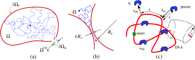
Figure 7: (a) The canonical narrow escape problem. A particle with diffusivity $D$ can escape from an asymptotically small aperture. The mean time $\langle T({\bf x})\rangle$ to escape $\Omega$, as a function of initial position ${\bf x}$ can be calculated in the asymptotic limit $\varepsilon\to 0$. (b) An escape problem where the escape hatch is at a cusp. (c) DNA target site search problem. Search is facilitated by 1D diffusion along the DNA chain.

A number of asymptotic results for the mean escape time of particles in confined geometries have been determined by Singer, Schuss, and Holcman [52], as well as Ward, et al.[53].

Figure 7(a) shows the diffusing particle in a volume $\Omega$ that can escape from a small hole of size $\sim\varepsilon\Omega^{1/d}$, where $d$ is the spatial dimensionality of $\Omega$. If $\varepsilon\ll 1$, estimates of the mean first exit times have been derived using asymptotic analysis of Eq. 10 and conformal mapping. Specifically, in 2D and 3D, for escape from a small hole punched through a smooth boundary as shown in Fig. 7(a), we find

$$\begin{array}[]{rlr}\langle T\rangle&\displaystyle\sim{\Omega\over 4\pi D}\left[\log{1\over\varepsilon}+O(1)\right],&\mbox{2D}\\[13.0pt] \langle T\rangle&\displaystyle\sim{\Omega^{2/3}\over\varepsilon D}\left[1+{\varepsilon\over\pi}\log{1\over\varepsilon}+\ldots\right].&\quad\mbox{3D}\end{array}$$ (25)

Analogous results were obtained for the constriction escape problem, where a narrow bottleneck is formed by circles or spheres of radius $R_{\rm c}$ approaching each other or revolved to form a three-dimensional bottleneck:

$$\begin{array}[]{rlr}\langle T\rangle&\displaystyle\sim{\pi\Omega\over 2D\sqrt{\varepsilon}},&\mbox{2D }\\[13.0pt] \langle T\rangle&\displaystyle\sim{\Omega\over\sqrt{2}R_{\rm c}D}{1\over\varepsilon^{3/2}},&\quad\mbox{3D}.\end{array}$$ (26)

Similar results have been derived for different geometries such as diffusion to the tip of a corner, and first passage to the end of a long neck. Due to the chosen geometries, escape is a rare event, and the particle reaches a quasi-steady-state distribution before any escape has occurred. Since the time to reach the quasi-steady-state distribution starting from a specific position is negligible compared to the mean escape time, all the above results are independent of the particle’s initial position ${\bf x}$.

Another related and biologically important example of first passage is the search of molecules for their target sites, such as the binding of transcription factors (sequence-specific DNA-binding proteins) to their corresponding binding sites along DNA [54, 55, 56, 57, 58] (see Fig. 7(c)). These sites are often proximal to the genes they regulate, although in reality, numerous transcription factors, including basal factors, RNA polymerase, coactivators, and activators must assemble before transcription of a specific gene is initiated. The search problem is of theoretical interest because experimental search times are much shorter than those estimated from simple 3D diffusion alone, leading to the idea of facilitated diffusion, a mechanism whereby more than one transport path is available. Since DNA is a linear, often compacted polymer, sections many bases away from the target may nonetheless be spatially proximal to it. These physical features have been incorporated into transport models to estimate the time it takes for an enzyme to bind its intended target along DNA of arclength $L$. The original phenomenological model assumes an effective absorbing sphere of radius $\lambda$ around the target, where $\lambda$ is the typical contiguous length traveled along the DNA. A simple heuristic expression for this “antennae effect” on the search time was derived: $\langle T\rangle\approx(L/\lambda)(\tau_{1}+\tau_{3})$, where $\tau_{1}$ and $\tau_{3}$ are the typical times spent on the DNA and in the bulk, respectively. To obtain realistic search times using this expression requires that the enzyme spend approximately an equal amount of time on DNA as in the bulk. However, in reality, enzymes spend an overwhelming majority of time associated with DNA. Moreover, this expression breaks down in certain singular limits such as when the one-dimensional diffusivity $D_{1}\to 0$, leading to $\tau_{1}\to\infty$. An improved expression for the mean search time has been recently derived [59],

$$\langle T\rangle\approx{Lr\over 2D_{3}n_{\rm p}}\left({r\over\lambda n_{\rm ad}}+{\lambda D_{3}n_{\rm p}\over D_{1}rn_{\rm ads}}+{2D_{3}k_{\rm off}\over k_{\rm on}D_{1}\sqrt{n_{\rm p}}}\right),$$ (27)

where $L$ is the arclength of the DNA, $r$ is its effective thickness, $n_{\rm p}$ and $n_{\rm ads}$ are the number of bulk and adsorbed proteins, and $k_{\rm on}$ and$k_{\rm off}$ are the attachment and detachment rates of protein. Note that in this treatment, $k_{\rm on}$ was defined using a reference protein concentration of one molecule per search volume. The typical arclength a protein stays within $r$ of the DNA before dissociating is thus estimated to be

$$\lambda\approx{r\sqrt{k_{\rm on}D_{1}}\over\sqrt{k_{\rm off}D_{3}n_{\rm ads}}}.$$ (28)

The result (28) is able to resolve a number of quantitative kinetic issues. In particular, Cherstvy, Kolomeisky, and Korynyshev[59] were able to find optimal binding energies that minimize the search time. Within a realistic parameter regime, the reduction in search time relative to 3D diffusion alone can be obtained even for small $D_{1}/D_{3}$. Additional details and references are found in Kolomeisky[60]. Note that all results on this problem are independent of the initial starting position of the searching enzyme since an initial uniform distribution of enzyme positions is implicitly assumed.

The molecular search problem is also intimately related to the filament growth described in the previous section. During mitosis, the ends of growing and shrinking microtubules emanating from centrosomal bodies form a party in search of kinetochores that hold together chromosomes [61, 62]. Using the Green’s function approach of Bicout [47] for a single microtubule as a starting point, Gopalakrishnan and Govindan [63] found estimates for the search time to one kinetochore

$$\langle T\rangle\approx{e^{\Delta d}\over p}\left(1+{f_{-}(1-e^{-\Delta d})\over v_{-}\Delta}\right)\left({v_{+}+v_{-}\over\Delta v_{-}v_{+}}+{1\over f}\right),$$ (29)

where $\Delta\equiv(v_{-}f_{+}-v_{+}f_{-})/(v_{+}v_{-})$, and $f$ is the frequency of nucleation of new microtubules from the centrosome that is located a distance $d$ from the kinetochore target. The probability that any new microtubule is pointed in the right direction and within the capture cone is $p\ll 1$. The microtubule velocities $v_{\pm}$ and flipping rates $f_{\pm}$ take on the same meaning as in Eq. 22 used by Bicout to study the lifetime of a single microtubule. Equation 29 holds only when the cell radius $R\gg d$. This and related formulae allow for an easy determination of optimal parameters that minimize the mean search time. The topic of capture of multiple kinetochores associated with multiple chromosomes has also been treated by Wollman et al. [62].

Besides the filament growth and search problems described in Section 3 and above, two other examples of cellular transport involving first passage times have been recently discussed: optimal microtubule transport of virus material to a host cell nucleus [64], and localization of DNA damage repair enzymes to DNA lesions [65, 66].

When a virus first enters a mammalian host cell its genetic material needs to be processed and transported into the host cell nucleus before productive infection can occur. The transport is often mediated by molecular motors that carry viral RNA or DNA towards the nucleus. This process was modeled by a unidirectional convection of cargo in multiple stages, while detachment of the motor and degradation of the viral cargo was implemented by a decay term. Nuclear entry probabilities and conditional first arrival times for cargo starting at the cell periphery and ending at the nucleus were calculated [64]. These were found to depend on parameters describing convection, decay, and transformation in nontrivial ways which suggested new strategies for drug intervention of the transport process.

Another biophysical example where finding first passage times is important is the localization of proteins to certain sites on DNA using an electron ejection mechanism [65]. A redox mechanism for certain DNA repair enzymes to localize near DNA damage sites has been proposed [67, 68, 69], as depicted in Fig. 8(a). Here, a recently deposited repair enzyme oxidizes by releasing an electron that can either scatter or absorb at guanine bases and damaged DNA sites. The oxidized repair enzyme has a higher binding affinity to DNA. However, if the electron returns, the reduced enzyme will dissociate from the DNA.

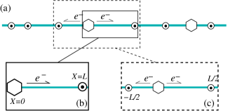
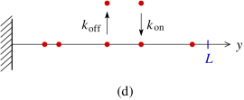
Figure 8: (a) A repair enzyme (hexagon) adsorbs onto a DNA which is initially populated by guanine radicals (circled dots) with a density $\rho$. An electron is emitted to the left or right with equal probability. The emitted electron has flip rates $f_{\pm}$, rightward/leftward velocity $v_{\pm}$ and decay rate $M$. (b) The one-sided Broadwell problem. An electron is emitted from position $X=0$ with probability $1$ toward a guanine radical at $X=L$. (c) The two-sided Broadwell problem. An enzyme is deposited between two guanine radicals which are at a distance $L$ apart. Immediately after landing inside this segment, an electron is emitted to the left or right with equal probability. (d) First passage time to a boundary position $y=L$ in the presence of multiple particles undergoing Langmuir kinetics.

Within this overall mechanism, the problems of the first electron return time, conditioned on its returning arises. The model equation for this subproblem is identical to Eq. 22 except that $x$, $v_{\pm}$, and $f_{\pm}$ are the position, speeds, and flip rates of an electron along the DNA, and decay terms are added to describe the absorption of electrons “off” the DNA. The effective desorption rate was calculated from the probability and time of electron return. For repair enzymes that land far from electron absorbing lesions, and if other electron-absorbing mechanisms are negligible, return of the emitted electron is likely and the enzyme will detach before it can diffuse sufficiently far. However, in a finite cell volume, the detached enzyme reenters the bulk pool and can reattach to the DNA, potentially closer to the lesion. Deposition near a lesion will likely be longer-lived because the ejected electron will be more likely absorbed rather than returning and dissociating the enzyme. In this way, Fok and Chou [65, 66] were able to find conditions under which the repair enzymes statistically localize near electron-absorbing damage sites on DNA.

Finally, search problems can involve multiple diffusing particles. In this case, it is still reasonable to define the state-space in terms of the positions $\{x_{j}\},\,1\leq j\leq N$ for each of, say, $N$ particles. In one-dimension, the first hitting time for any particle to reach an absorbing point of a line segment has been examined by Sokolov et al.[70] who considered noninteracting particles that diffuse and undergo Langmuir kinetics as shown in Fig. 8(b). In their study, the authors employ a mean-field assumption for Eq. 4 where the probability current $J(t)$ is conditioned on no other particle having exited the interval previous to time $t$. The mean-field assumption arises by expressing this conditioning as $J_{\rm conditioned}(t)=J_{\rm unconditioned}S(t)$. The mean-field solution to the probability $S(t)$ that no particle has hit the target site up to time $t$ is

$$S(t)=J(t)\exp\left[-\int_{0}^{t}J(t^{\prime})\mbox{d}t^{\prime}\right],$$ (30)

where $J(t)$ is the unconditioned probability flux. Note that for this approximation to yield physical results, we require

$$\lim_{t\to\infty}tJ(t)>0$$ (31)

in order for $\int_{0}^{t}J(t^{\prime})\mbox{d}t^{\prime}$ to diverge and $S(t)\to 0$ as $t\to\infty$. In this problem, the flux was approximated by $J(t)=-D\partial_{y}n(y,t)|_{y=L}$, where $n(y,t)$ is the particle density at position $y$ that is found from

$${\partial n(x,t)\over\partial t}=D{\partial^{2}n(x,t)\over\partial x^{2}}-k_{\rm off}n+k_{\rm on},$$ (32)

where $D$ is the one-dimensional diffusivity, and $k_{\rm on}$ and $k_{\rm off}$ are the particle adsorption and desorption rates. Because of the implied infinite bulk reservoir (through rate $k_{\rm on}$) the mean-field flux satisfies Eq. 31. Even in the case $k_{\rm off}=k_{\rm on}=0$, if an infinite system size is assumed, the condition in Eq. 31 is also satisfied. In fact, when the system is infinite, the mean-field assumption in Eq. 30 is exact.

A more general approach that does not initially rely on the mean-field assumption, and can be used for finite-sized systems, is to note that if the particles are noninteracting, the survival probability $S(t;\{x_{i}\})=\prod_{i=1}^{N}S_{1}(t;x_{i})$ is a product of the survival probabilities of each particle with initial position $x_{i}$. We assume a finite segment and assume $N$ total of particles, including those in the bulk. In this way, we can compute the single particle probability flux $J_{1}(t)=-D\partial_{y}P_{1}(y,t|x,0)|_{y=L}$, and use the exact relation

$${\partial S_{1}(t;x)\over\partial t}=-J_{1}(t;x)=D\partial_{y}P_{1}(y,t|x,0)|_{y=L}.$$ (33)

Using conservation of probability, $\int_{0}^{\infty}J_{1}(t^{\prime};x)\mbox{d}t^{\prime}=1$ and, assuming the initial positions (including the possibility of being detached from the lattice) of all particles are identical, we find

$$S(t;x)=\left[1-\int_{0}^{t}J_{1}(t^{\prime};x)\mbox{d}t^{\prime}\right]^{N}.$$ (34)

A direct comparison can be made with the mean field result in the case $k_{\rm off}=k_{\rm on}=0$. Upon solving Eq. 32, we can find the the Laplace transform of the single-particle probability flux, assuming a uniformly distributed initial condition

$$\tilde{J}_{1}(s)=-D{\partial\tilde{n}(x,s)\over\partial x}\bigg{|}_{x=L}={\tanh L\sqrt{s/D}\over L\sqrt{s/D}}.$$ (35)

Upon inverse Laplace-transforming, and using the result in Eq. 34, we can find the exact survival probability. Note that this result is different from using $NJ_{1}(t)$ for $J(t)$ in the mean-field approximation Eq. 30. Only in the infinite system size limit of $L,N\to\infty$, but $N/L=n_{0}$ constant do the mean-field and exact result $S(t)=\exp\left[-2n_{0}\sqrt{Dt/\pi}\right]$ coincide. This can be shown mathematically by using $L=N/n_{0}$ in Eq. 35, inverse Laplace transforming, substituting the result in Eq. 34, and taking the $N\to\infty$ limit. The discrepancy can be most easily seen by assuming all particles start at $x$ and

$${\partial S(t;x)\over\partial t}=NS_{1}^{N-1}(t;x){\partial S_{1}(t;x)\over\partial t}=-NJ_{1}(t;x)S_{1}^{N-1}(t;x).$$ (36)

For noninteracting particles, the total annihilation flux $J(t;x)=NJ_{1}(t;x)$, and

$${\partial S(t;x)\over\partial t}=-J(t;x)S_{1}^{N-1}(t;x)=-J(t;x){S(t;x)\over S_{1}(t;x)}.$$ (37)

The relative effect of the extra factor $S_{1}(t;x)<1$ on $S(t;x)$ decreases as $N\to\infty$. It should be stressed that independence of the diffusing particles allow for the exact analysis above. However, certain approximate results for interacting particles have also been obtained [71].

Multiple particle first passage problems also illustrate the concept of order statistics. Although Eq. 34 provides the survival probability of a boundary untouched by any one of the diffusing particles, one might be interested in the statistics of the first, second, third, etc., particle to leave the interval, as well as the complete clearing time distribution. These order statistics and asymptotic expressions for the first two moments of the $j$ exit times have been derived for independent particles diffusing in one-dimension [72] and $d-$dimensions [73].

5 Neuronal Spike Trains

An important first passage problem within a living, functioning nerve cell, or group of nerve cells arises in the study of the timing of electrical spike trains. While modeling the stochastic dynamics of the membrane potential of a neuron requires taking into account a large number of detailed microscopic processes, such as nonlinear ion channel gating and membrane capacitance and leakage, the overall phenomena of spike trains can be effectively described by a stochastic process with a threshold membrane potential $V^{*}$. When the voltage of a neuron reaches $V^{*}$, highly nonlinear processes take over, the voltage quickly spikes, and returns to a reset voltage, as shown in Fig. 9(a). The interspike times are distributed according to the time that the transmembrane potential first reaches $V^{*}$ after the previous resetting.

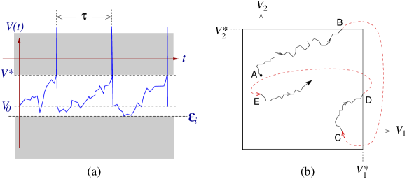
Figure 9: First exit times in simple neuronal firing models. (a) A schematic time trace of the transmembrane potential showing voltage spikes triggered at $V^{*}$ and resetting back to $V_{0}$. The subthreshold voltage dynamics is a stochastic processes with the interspike time distribution measuring the statistics of the first passage time to the threshold voltage. (b) Voltage trajectories for two coupled neurons, with transmembrane voltage $V_{1}$ and $V_{2}$. If neuron 2 spikes first at point (B), $V_{2}$ spikes and quickly resets to point (C). In this example, neuron 1 spikes next at point (D), and $V_{1}$ resets to point (E).

A simple one-dimensional stochastic model for predicting interspike times for a single neuron has been proposed by Stein [74]. Here, the transmembrane voltage is assumed to dissipate through a “leak” current, while other connected neurons impart noise to the neuron of interest. The model implicitly relies on a mean field assumption in the sense that none of the other neurons are affected by the behavior of the neuron in question. The “bath” neurons provide random excitatory and inhibitory signals through unspecified physical connections with the isolated neuron. Starting from a stochastic differential equation (SDE) formulation, increments of the transmembrane voltage $V$ can be expressed as

$$\mbox{d}V=-{V\over\tau}\mbox{d}t+a_{\rm e}\mbox{d}\pi_{\rm e}(r_{\rm e},t)-a_{\rm i}\mbox{d}\pi_{\rm i}(r_{\rm i},t),$$ (38)

where $a_{\rm e}$ and $a_{\rm i}$ are the fixed amplitudes of the excitatory and inhibitory spikes feeding into the neuron, and $\pi_{\rm e}(r_{\rm e},t)$ and $\pi_{\rm i}(r_{\rm i},t)$ are possibly time-varying unit excitatory and inhibitory Poisson processes with rates $r_{\rm e}$ and $r_{\rm i}$, respectively. Suppose the voltage starts at $V(t=0)=X$ and that the threshold for spiking is $V_{*}$. The recursion equations for the moments $M_{n}(X;V_{*})\equiv\langle T^{n}(X;V_{*})\rangle$ of the interspike times are [75]

$${X\over\tau}{\mbox{d}M_{n}\over\mbox{d}X}-r_{\rm e}M_{n}(X+a_{\rm e})-r_{\rm i}M_{n}(X-a_{\rm i})+(r_{\rm e}+r_{\rm i})M_{n}(X)=nM_{n-1}(X),$$ (39)

where $M_{0}(X)\equiv 1$. The mean interspike times $M_{1}(X,V_{*})\equiv\langle T(X)\rangle$ were analyzed by Cope and Tuckwell [76] using asymptotic analysis for large negative reset voltages, and continuing the solutions to the threshold $V_{*}$. Assuming $a_{\rm e}=a_{\rm i}$, their result for the mean first time $T(V)$ to spiking starting from an initial voltage $V$ can be expressed in the form

$$\langle T(X,V_{*})\rangle\approx{1\over r_{\rm e}}\left[{1\over\tau r_{\rm e}}\log\left({V\over a_{\rm e}}\right)+C\left({V_{*}\over a_{\rm e}}\right)+\sum_{n=1}^{\infty}A_{n}\left({a_{\rm e}\over V}\right)\right],$$ (40)

where the function $C(V_{*}/a_{\rm e})$ and the coefficients $A_{n}$ were numerically found from recursion relations of a set of linear equations. However, note that the associated equation for the voltage probability density $P(V,t|V_{0},0)\mbox{d}V$ is

$${\partial P\over\partial t}={1\over\tau}{\partial(VP)\over\partial V}+r_{\rm e}P(V-a_{\rm e},t)+r_{\rm i}P(V+a_{\rm i},t)-(r_{\rm e}+r_{\rm i})P,$$ (41)

where only arguments of $P$ that are different from $(V,t|V_{0},0)$ are explicitly written. A further simplification can be taken by assuming the noise amplitudes $a_{\rm e,i}$ are small and Taylor expanding the probability densities to second order in $a_{\rm e,i}$ (a “diffusion” approximation). The Fokker-Planck or Smoluchowski equation now takes the form

$${\partial P\over\partial t}={\partial\over\partial V}\left[\left({V\over\tau}-r_{\rm e}a_{\rm e}+r_{\rm i}a_{\rm i}\right)P\right]+{1\over 2}\left(r_{\rm e}a_{\rm e}^{2}+r_{\rm i}a_{\rm i}^{2}\right){\partial^{2}P\over\partial V^{2}},$$ (42)

with $P(V,t|V_{0},0)=\delta(t)$ when $V=V_{*}$. This model for subthreshold neuron voltage is simply a first passage problem of the Ornstein-Ulhenbeck process that has been used to describe particle escape from a quadratic potential or rupturing of a harmonic bond. Recasting the problem using a Backward Kolmogorov Equation, the survival probability (the probability that no spike has occurred) as well as the moments of the interspike times can be expressed in terms of special functions [75]. Tuckwell and Cope [75] also provide a careful analysis of the accuracy of the diffusion approximation in approximating the “exact” results from Eq. 39. As expected the diffusion approximation is accurate in the limit of large excitatory and inhibitory spike noise rates $r_{\rm e}$ and $r_{\rm i}$, and when the threshold voltage $V_{*}$ is far from the reset voltage.

Besides simple one-dimensional models, higher dimensional models that include more mechanistic details of a single neuron have also been studied. In particular, stochastic first passage problems for Fitzhugh-Nagumo [77] and Hodgkin-Huxley models [78] have been developed. These more complex models still focus on the voltage dynamics of a single neuron, with the voltage dynamics of other connected neurons subsumed into the “noise” felt by the neuron. Typically, the multiple neuron voltages can be simultaneously measured using multielectrode recordings, allowing for the quantification of the correlations between the spiking times of connected neurons. A first approach for modeling these higher dimensional data is to treat the stochastic dynamics of a small number of interacting neurons. For the two neuron problem illustrated in Fig. 9(b), the dynamics of the subthreshold voltages of neurons 1 and 2, $V_{1}$ and $V_{2}$, respectively, are independent of each other, and the probabilities factorize: $P(V_{1},V_{2})\mbox{d}V_{1}\mbox{d}V_{2}=P_{1}(V_{1})P_{2}(V_{2})\mbox{d}V_{1}\mbox{d}V_{2}$. Interactions between the two neurons occur when either voltage spikes. A neuron connected to one that spikes can suffer a small voltage displacement. Rather than treating each neuron as subject to independent noise, the spiking time statistics of the neurons provide one component of the random noise of the other neuron. The full spiking time statistics must be computed self-consistently. Trajectories in the state space shown in Fig. 9(b) can be described moving along a torus with jumps in the orthogonal direction each time it crosses circumferentially or axially. Mathematically, the probability densities for the two subthreshold voltages obey

$${\partial P_{i}(V_{i},t)\over\partial t}={\partial\over\partial V_{i}}\left[U_{i}(V_{i})P_{i}\right]+D_{i}{\partial^{2}P_{i}\over\partial V_{i}^{2}},$$ (43)

where $D_{i}$ is the voltage diffusivity in neuron $i$. However, as soon as one $V_{i}$ reaches $V_{i}^{*}$, not only does it reset, but $V_{j\neq i}\to V_{j\neq i}+\delta_{j}$ is shifted by $\delta_{j}$.

6 Cellular and organismic population dynamics

The simplest nonspatial deterministic population model, describing growth limitations due to a carrying-capacity, centers on the logistic equation

$${\mbox{d}n(t)\over\mbox{d}t}=rn(t)\left(1-{n(t)\over K}\right),$$ (44)

where $n(t)$ is the population density and $K$ is the carrying-capacity. This deterministic model has stable fixed points at $n=0$ and $n=K$. There are multiple ways to define stochastic birth-death models that in the mean field limit reduce to Eq. 44 [79]. Nonetheless, all of these models requires at least one existing organism for proliferation to take place. Therefore, these models contain an absorbing state at $n=0$, where the population is extinct. Although the deterministic equation predicts, at long times, a permanent population $n=K$, a stochastic model predicts a finite extinction time $T$ after which $n(t\geq T)=0$. Approximations to this extinction time have been analyzed by Kessler and Shnerb [80] using a WKB approximation and Assaf and Meerson [81] using a generating function approach and properties of the associated Sturm-Liouville equation. Both methods use the approximation $K\gg 1$, for which extinction is rare, and a near equilibrium number distribution is first achieved before an extinction event occurs. This approximation is analogous to that of assuming “local thermodynamic equilibrium” (as opposed to kinetic theory) for transport calculations [82]. The probability flux is then constructed from the rate of transport into an absorbing state from this near equilibrium density. The distribution of times for the rare extinction events are nearly exponential

$$w(t)\mbox{d}t\approx\Gamma e^{-\Gamma t}\mbox{d}t,$$ (45)

where to leading order the extinction rate is of the form

$$\Gamma\sim K^{3/2}e^{-K}.$$ (46)

Note that these results, as with those of the narrow escape problem (Section 4), do not depend on the initial number $n_{0}=n(t=0)$ because equilibration to a quasi-stationary state occurs on a time scale much faster than $\Gamma^{-1}$.

Other classic population models, such as models for cell genotype/phenotype populations, Lotka-Volterra type models [83], and disease models (such as SIS and SIR)[84, 85] have also been extended into the stochastic realm, and the corresponding exit times into absorbing configurations analyzed (see Ovaskainen and Meerson[86] for a review). Here, the total organism number is a random variable determined by the dynamical rules of the model, which may include “interacting” effects such as carrying-capacity. The simplest model for heterogeneity in a birth-death process is the Wright-Fisher model or, in continuous-time, the Moran model. The latter is a stochastic model for two-competing species with numbers $n_{1}$ and $n_{2}$, where the total population $n_{1}+n_{2}\equiv N$ is fixed. Since $n_{2}=N-n_{1}$, the problem state-space reduces to one-dimension. The transition rules in the Moran model are defined by randomly selecting an individual for annihilation, but instantaneously replacing it with either one of the same type (so that the system configuration does not change), or one of the opposite type. The transition probability in time interval $\mbox{d}t$ for converting an $n_{1}$ individual to an $n_{2}$ individual is thus $r_{1}n_{1}n_{2}\mbox{d}t=r_{1}n_{1}(N-n_{1})\mbox{d}t$, while conversion of $n_{2}$ to $n_{1}$ occurs with probability $r_{2}n_{2}(N-n_{2})\mbox{d}t$. By defining $P(n,t|m,0)$ as the probability that there are $n=n_{1}$ type 1 individuals at time t, given that there were initially $m$ type 1 individuals, the BKE is simply

$$\begin{array}[]{rl}\displaystyle{\partial P(n,t|m,0)\over\partial t}=&\displaystyle m(N-m)\big{[}r_{1}P(n,t|m+1,0)+r_{2}P(n,t|m-1,0)\\[13.0pt] &\hskip 93.95122pt-(r_{1}+r_{2})P(n,t|m,0)\big{]}.\end{array}$$ (47)

Note that $n=0$ and $n=N$ are absorbing states corresponding to the entire population being fixed to either type 1 or type 2 individuals. Upon summing $\sum_{n=1}^{N-1}P(n,t|m,0)\equiv S(t;m)$, we can find the corresponding BKE for the probability of survival against fixation at either $n=0$ or $n=N$. The mean time to fixation can then be found from inverting the matrix equation

$$m(N-m)\left[r_{1}\langle T(m+1)\rangle+r_{2}\langle T(m-1)\rangle-(r_{1}+r_{2})\langle T(m)\rangle\right]=-1,$$ (48)

with $\langle T(0)\rangle=\langle T(N)\rangle=0$, to give the well-known result

$$\langle T(m)\rangle=N\sum_{k=1}^{m}{N-m\over N-k}+N\sum_{k=m+1}^{N-1}{m\over k}.$$ (49)

If spontaneous mutations are included in the model, there is strictly no fixation since the states $n=0,N$ are no longer absorbing. Many generalizations of the Moran model have been investigated, including extensions to include more species, fluctuating population sizes, and time-dependent parameters such as the rates $r_{1}(t),r_{2}(t)$ [87, 88]. These extended models are not typically amenable to closed form solutions such as Eq. 49. Nonetheless, it is often possible to employ asymptotic analysis in the large $N$ limit and derive a corresponding PDE for either the probability density or its generating function. For example, if one assumes $N\to\infty$ and takes $x=m/N$ one finds the diffusion approximation for the BKE

$${\partial S(t;x)\over\partial t}=D_{\rm eff}x(1-x){\partial^{2}S(t;x)\over\partial x^{2}},\quad 0\leq x\leq 1.$$ (50)

Here, we have introduced $D_{\rm eff}=r_{1}N^{2}=r_{2}N^{2}$. The corresponding PDEs for more complex Moran-type models are often amenable to analysis, making the Moran model one of the paradigmatic theories in population biology and ecology. However, recall from Section 1 the discrepancy between the first passage times derived from discrete and corresponding continuum theories [6]. For Eq. 50, there is no selection or mutation giving rise to a convection term, so the corresponding mean first passage time asymptotically approaches the discrete result in Eq. 49 as $N\to\infty$. However, care should be exercised for more complex models that include effective convection terms.

Higher dimensional generalizations of these types of discrete models can also be readily applied to problems in cell population biology such as cancer modeling and stem-cell proliferation. When the total population size constraint is relaxed, a linear, multiple state model shares many mathematical features with the Zero-Range Process (ZRP) [89], as shown in Fig. 10. The multiple sites in such a ZRP might represent the number of cells in a tissue at a particular mutation stage as the cells progress towards a cancerous state. Of interest is the first time that a certain number of cells arrive at the final, “fully cancerous” state .

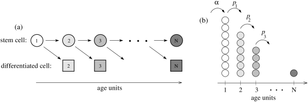
Figure 10: Schematic of a reduced model of stem-cell aging. (a) Asymmetric division of aging stem-cells. The circles represent stem cells, while the squares represent differentiated cells. The numerical index represents the age of the cell and is assumed to be inversely related to the telomere length. (b) A lattice representation of the stem-cell aging model. The rate of asymmetric differentiation are shown as $p_{k}$, while the death rates $\mu_{k}$ at each age $k$ are not indicated.

Besides multi-hit models of cancer and evolution, the Zero-range process can also be adapted to model aging in a stem-cell population. Consider stem-cells that have a limited number of divisions due to shortening telomeres, ends of their DNA that are shortened at each division. Without telomerase to rebuild these ends, cells will generally be programmed for death. As shown in Fig. 10(a), our model assumes that each division leads to one stem-cell and one differentiated cell, both aged by one unit (or both with shortened telomeres). Since all cell divisions are asymmetric, yielding one stem-cell and one differentiated cell, one only needs to keep track of the number of stem-cells. The forward master equation for the process has been derived in Shargel, D’Orsogna, and Chou [90], as well as the associated equation for the generating function:

$$\frac{\partial G}{\partial t}=-\sum_{j=1}^{N-1}(\mu_{j}+p_{j})z_{j}{\partial G\over\partial z_{j}}+\sum_{j=1}^{N}\mu_{j}{\partial G\over\partial z_{j}}+\sum_{j=1}^{N-1}p_{j}z_{j}{\partial G\over\partial z_{j}}-\mu_{N}z_{N}{\partial G\over\partial z_{N}},$$ (51)

where

$$G(z_{1},\cdots,z_{N};t)=\sum_{n_{j}}P(n_{1},\cdots,n_{N};t)z_{1}^{n_{1}}\cdots z_{N}^{n_{N}}$$ (52)

and $P(\{n\};t)$ is the probability that there are exactly $n_{k}$ stem-cells of age $k$ at time $t$. If we do not assume an immigration of new stem-cells defined as having age $k=1$ (as was done in Shargel, D’Orsogna, and Chou[90]), Eq. 51 can be expressed in the form $\mbox{d}G/\mbox{d}t=0$ and solved using the method of characteristics. The vector of characteristic trajectories ${\bf Z}=(z_{1},z_{2},\ldots,z_{N})^{T}$ can be found by solving $\dot{{\bf Z}}={\bf P}{\bf Z}-{\bf M}$, where

$${\bf P}=\left[\begin{array}[]{ccccc}\mu_{1}+p_{1}&-p_{1}&0&\cdots&0\\ 0&\mu_{2}+p_{2}&-p_{2}&\cdots&0\\ 0&\cdots&\mu_{j}+p_{j}&-p_{j}&0\\ 0&\cdots&0&\mu_{N-1}+p_{N-1}&-p_{N-1}\\ \cdots&\cdots&\cdots&\cdots&\cdots\\ 0&\cdots&0&0&\mu_{N}\end{array}\right]$$ (59)

and ${\bf M}=(\mu_{1},\cdots,\mu_{j},\cdots,\mu_{N})^{T}$. For an initial condition of one stem-cell of age $k=1$, these trajectories can be inverted and expressed in terms of the initial values $z_{i}(t=0)$, which form the independent variable in the generating function:

$$G({\bf Z};t) = z_{1}e^{-\Delta_{1}t}+\sum_{i=2}^{N}\left[z_{i}(-1)^{i+1}\left(\prod_{\ell=1}^{i-1}p_{\ell}\right)\sum_{j=1}^{i-1}\frac{e^{-\Delta_{j}t}-e^{-\Delta_{i}t}}{\prod_{k\neq j}^{i}(\Delta_{j}-\Delta_{k})}\right]+$$

$$1-e^{-\Delta_{1}t}+\sum_{i=2}^{N}\left[(-1)^{i}\left(\prod_{\ell=1}^{i}p_{\ell}\right)\sum_{j=1}^{i-1}\frac{e^{-\Delta_{j}t}-e^{-\Delta_{i}t}}{\prod_{k\neq j}^{i}(\Delta_{j}-\Delta_{k})}\right],$$

where $\Delta_{j}\equiv p_{j}+\mu_{j}$, for $1\leq j\leq N-1$ and $\Delta_{N}=\mu_{N}$. From the generating function in Eq. 6 we can derive the probability $P(n_{1}=0,...,n_{j}=1,...,n_{N}=0;t)$ that a certain age by the descendants of single cell can be found at a given age $j$:

$$P(n_{1}=1,n_{2}=0,\cdots,n_{N}=0)=e^{-\Delta_{1}t},$$ (61)

while for all other ages $1<j<N$ we find

$$\begin{array}[]{rl}P(0,\cdots,n_{j}=1,\cdots,0;t)&\displaystyle=(-1)^{j}\left(\prod_{\ell=1}^{j-1}p_{\ell}\right)\sum_{k=1}^{j-1}\frac{e^{-\Delta_{j}t}-e^{-\Delta_{k}t}}{\prod_{i\neq k}^{j}(\Delta_{k}-\Delta_{i})}\\[13.0pt] &=\displaystyle{(pt)^{j-1}\over(j-1)!}e^{-(\mu+p)t},\end{array}$$ (62)

where the last equality holds in the case where all $p_{i}=p$ and $\mu_{i}=\mu$ are age-independent. Finally, the probability for complete extinction of the lineage is given by

$$P(\{n\}=0;t)=1-e^{-\Delta_{1}t}+\!\sum_{i=2}^{N}\left[(-1)^{i}\left(\prod_{\ell=1}^{i-1}p_{\ell}\right)\sum_{j=1}^{i-1}\frac{e^{-\Delta_{j}t}-e^{-\Delta_{i}t}}{\prod_{k\neq j}^{i}(\Delta_{j}-\Delta_{k})}\right].$$ (63)

It can be easily verified that the sum of the probabilities in Eqs. 61, 62 and 63 add to unity, and that $P(n_{1}=0,\cdots,n_{N}=0;t\to\infty)\to 1$, indicating that a single cell will eventually age and that its lineage will go extinct with certainty.

From these probabilities we can construct the probability that the oldest age reached by a lineage is $Q_{k}$:

$$Q_{k}=\int_{0}^{\infty}\!\!\left[p_{k-1}P(0,...,n_{k-1}=1,...,0;t)-p_{k}P(0,...,n_{k}=1,...,0;t)\right]\mbox{d}t.$$ (64)

Equation 64 is derived by considering the difference between the probability flux into age $k$ and the flux out of age $k$ into age $k+1$ (excluding death). The time-integrated result $Q_{k}$ is thus the probability that the lineage died at age $k$. For the constant rate case $p_{i}=p$ and $\mu_{i}=\mu$, we find explicitly

$$Q_{1}={\mu\over\mu+p},\quad Q_{k}={\mu p^{k-1}\over(\mu+p)^{k}},\,\,\,\mbox{and}\,\,\,Q_{N}={p^{N-1}\over(\mu+p)^{N-1}}.$$ (65)

From these probabilities, we can define the first passage time to age $k$ conditioned on the system reaching at least age $k$. Since the decay at all ages preceding $k$ are “interfering” absorbing states, we can use $J_{1}^{k}(t)=pP(0,...,n_{k-1}=1,...,0;t)$ in Eq. 11 to find

$$w_{1}(t|k)\equiv J_{1}(t|k)={(\mu+p)((\mu+p)t)^{k-2}\over(k-2)!}e^{-(\mu+p)t},\quad k\geq 2,$$ (66)

with a corresponding conditional mean arrival time to age $k$: $\langle T_{1}(k)\rangle=(k-1)/(\mu+p)$. Note that if the decay rate $\mu$ is high, the conditional mean arrival time is small because only fast trajectories will survive to state $k$.

Our simple stem-cell aging model assumes all divisions are asymmetric at all ages. Nonetheless, this model serves as an illustrative example of an application of a simple Markov process to cell biology. Indeed, since aging only increases, our model can also be represented by a simple asymmetric, decaying random walk of a single “particle” in one-dimension, with the position of the particle representing the age of the single stem-cell in the system at any given time. The more complicated approach we have illustrated above allows our model to be generalized to include effects of multiple initial stem-cells and symmetric stem-cell division, as well as a more complete analysis of differentiated cell populations.

7 Summary

We have surveyed only a few mathematical and physical models wherein first passage problems play a central role in the quantitative understanding of biological observations and experiments. These applications span all scales from molecular to cellular to populations. Most applications thus far have been concerned with low dimensional models with few degrees of freedom. As measurements improve and more complex systems can be quantitatively studied, first passage time problems should become increasingly important in higher dimensional settings where additional analytic and numerical insights will be desired. Furthermore, first passage problems provide a new framework with which to fit experimental data, model biological processes, and develop inverse problems of model determination.

8 Acknowledgments

The authors are grateful to B. van Koten, J. Newby, and J. J. Dong for incisive discussions and comments. This work was supported by the NSF through grants DMS-1021818 (TC) and DMS-1021850 (MD). TC is supported by the Army Research Office through grant 58386MA. MD was also supported by an Army Research Office MURI grant W911NF-11-1-0332.

References

- 1. S. Redner, A Guide to First-Passage Processes. Cambridge University Press, Cambridge, UK (2001).
- 2. K. B. Athreya and P. E. Ney, Branching Processes. Dover, Mineola, NY (2000).
- 3. T. E. Harris, The Theory of Branching Processes. Dover, Mineola, NY (1989).
- 4. G. H. Weiss, First passage time problems for one-dimensional random walks, Journal of Statistical Physics. 24(4), 587–594 (1981).
- 5. P. A. Pury and M. O. Caceres, Mean first-passage and residence times of random walks on asymmetric disordered chains, Journal of Physics A: Mathematical and General. 36, 2695 (2003).
- 6. C. R. Doering, K. V. Sargsyan, and L. M. Sander, Extinction times for birth-death processes: Exact results, continuum asymptotics, and the failure of the Fokker–Planck approximation, Multiscale Model. Simul. 3, 283–299 (2005).
- 7. G. I. Bell, Models for the specific adhesion of cells to cells, Science. 200, 618–627 (1978).
- 8. A. G. Nobile, L. M. Ricciardi, and L. Sacerdote, Exponential trends of Ornstein-Ulhenbeck first passage-time densities, Journal of Applied Probability. 22, 360–369 (1988).
- 9. L. M. Ricciardi and S. Sato, First-passage-time density and moments of the Ornstein-Uhlenbeck process, Journal of Applied Probability. 25(1), 43–57 (1988).
- 10. E. Evans, Probing the relation between force-lifetime-and chemistry in single molecular bonds, Annual Reviews in Biophysics and Biomolecular Structure. 30, 105–128 (2001).
- 11. E. A. R. Bizzarri and S. Cannistraro, Dynamic Force Spectroscopy and Biomolecular Recognition. CRC Press, Taylor and Francis Grp, LLC, Boca Raton, FL (2012).
- 12. C. W. Gardiner, Handbook of Stochastic Methods: For Physics, Chemistry, and the Natural Sciences. Springer, Berlin (2004).
- 13. J. Shillcock and U. Seifert, Escape from a metastable well under a time-ramped force, Phys. Rev. E. 57, 7301–7304 (1998).
- 14. B. E. Shapiro and H. Qian, A quantitative analysis of sinhle protein-ligand complex separation with the atomic force microscope, Biophysical Chemistry. 67, 211–219 (1997).
- 15. B. E. Shapiro and H. Qian, Hysteresis in force probe measurements: a dynamical systems perspective, J. theor. Biol. 194, 551–559 (1998).
- 16. H. Qian and B. E. Shapiro, Graphical method for force analysis: Macromolecular mechanics with atomic force microscopy, Proteins: Structure, Function, and Genetics. 37, 576–581 (1999).
- 17. G. Hummer and A. Szabo, Kinetics from nonequilibrium single-molecule pulling experiments, Biophysical Journal. 85, 5–15 (2003).
- 18. O. K. Dudko, A. E. Filippov, J. Klafter, and M. Urbach, Beyond the conventional description of dynamics force spectroscopy of adhesion bonds, Proc. Natl. Acad. Sci. USA. 100, 11378–11381 (2003).
- 19. A. Fuhrmann, D. Anselmetti, and R. Ros, Refined procedure of evaluating experimental single-molecule force spectroscopy data, Physical Review E. 77, 031912 (2008).
- 20. S. Getfert, M. Evstigneev, and P. Reimann, Single-molecule force spectroscopy: practical limitations beyond Bell’s model, Physica A. 388, 1120–1132 (2009).
- 21. L. B. Freund, Characterizing the resistance generated by a molecular bond as it is forcibly separated, Proc. Natl. Acad. Sci. USA. 106, 8818–8823 (2009).
- 22. A. Fuhrmann and R. Ros, Single-molecule force spectroscopy: a method for quantitative analysis of ligand-receptor interactions, Nanomedicine. 5, 657–666 (2010).
- 23. V. K. Gupta and C. D. Eggleton, A theoretical method to determine unstressed off-rate from multiple bond force spectroscopy, Colloids and Surfaces B: Biointerfaces. 95, 50–56 (2012).
- 24. V. K. Gupta, Rupture of single receptor-ligand bonds: A new insight into probability distribution function, Colloids and Surfaces B: Biointerfaces. 101, 501–509 (2013).
- 25. G. Bal and T. Chou, On the reconstruction of diffusions using a single first-exit time distribution, Inverse Problems. 20, 1053–1065 (2004).
- 26. P.-W. Fok and T. Chou, Reconstruction of bond energy profiles from multiple first passage time distributions, Proc. Roy. Soc. A. 466, 3479–3499 (2010).
- 27. T. P. J. Knowles, C. A. Waudby, G. L. Devlin, S. I. A. Cohen, A. Aguzzi, M. Vendruscolo, E. M. Terentjev, M. E. Welland, and C. M. Dobson, An analytical solution to the kinetics of breakable filament assembly, Science. 326, 1533–1537 (2009).
- 28. D. Sept and A. J. McCammon, Thermodynamics and kinetics of actin filament nucleation, Biophysical Journal. 81, 667–674 (2001).
- 29. J. Miné, L. Disseau, M. Takahashi, G. Cappello, M. Dutreix, and J.-L. Viovy, Real-time measurements of the nucleation, growth and dissociation of single Rad51-DNA nucleoprotein filaments, Nucleic Acids Res. 35, 7171–7187 (2007).
- 30. L. Edelstein-Keshet and G. Ermentrout, Models for the length distributions of actin filaments: I. simple polymerization and fragmentation, Bulletin of Mathematical Biology. 60, 449–475 (1998).
- 31. M. F. Bishop and F. A. Ferrone, Kinetics of nucleation-controlled polymerization. a perturbation treatment for use with a secondary pathway, Biophysical Journal. 46, 631–644 (1984).
- 32. E. T. Powers and D. L. Powers, The kinetics of nucleated polymerizations at high concentrations: amyloid fibril formation near and above the “supercritical concentration, Biophysical Journal. 91, 122–132 (2006).
- 33. D. Endres and Z. A., Model-based analysis of assembly kinetics for virus capsids or other spherical polymers, Biophysical Journal. 83, 1217–1230 (2002).
- 34. A. Zlotnick, Distinguishing reversible from irreversible virus capsid assembly, Journal of Molecular Biology. 366, 14–18 (2007).
- 35. A. Y. Morozov, R. F. Bruinsma, and R. J., Assembly of viruses and the pseudo-law of mass action, Journal of Chemical Physics. 131, 155101 (2009).
- 36. K. A. Brogden, Antimicrobial peptides: pore formers or metabolic inhibitors in bacteria?, Nature Reviews Microbiology. 3, 238–250 (2005).
- 37. G. L. Ryan and A. D. Rutenberg, Clocking out: Modeling phage-induced lysis of escherichia coli, J. Bacteriology. 189, 4749–4755 (2007).
- 38. M. R. D’Orsogna and T. Chou, First passage and cooperativity of queueing kinetics, Physical Review Letters. 95, 170603 (2005).
- 39. G. Bel, B. Munsky, and I. Nemenman, The simplicity of completion time distributions for common complex biochemical processes, Physical Biology. 7, 016003 (2010).
- 40. M. Ehrlich, W. Boll, A. van Oijen, K. Hariharan R., Chandran, M. L. Nibert, and T. Kirchhausen, Endocytosis by random initiation and stabilization of clathrin-coasted pits, Cell. 118, 591–605 (2004).
- 41. B. I. Shraiman, On the role of assembly kinetics in determining the structure of clathrin cages, Biophysical Journal. 72, 953–957 (1997).
- 42. L. Foret and P. Sens, Kinetic regulation of coated vesicle secretion, Proc. Natl. Acad. Sci. USA. 105, 14763–14768 (2008).
- 43. M. R. D’Orsogna, G. Lakatos, and T. Chou, Stochastic self-assembly of incommensurate clusters, Journal of Chemical Physics. 126, 084110 (2012).
- 44. R. Yvinec, M. R. D’Orsogna, and T. Chou, First passage times in homogeneous nucleation and self-assembly, Journal of Chemical Physics. 137, 244107 (2012).
- 45. M. R. D’Orsogna, B. Zhao, B. Berenji, and C. T., Combinatory analysis of heterogeneous stochastic self-assembly, Journal of Chemical Physics. 139, 121918 (2013).
- 46. R. J. Rubin, Mean lifetime of microtubules attached to nucleating sites, Proc. Natl. Acad. Sci. USA. 85, 446–448 (1988).
- 47. D. J. Bicout, Green’s functions and first passage time distributions for dynamic instability of microtubules, Phys. Rev. E. 56, 6656–6667 (1997).
- 48. D. J. Bicout and R. J. Rubin, Classification of microtubule histories, Phys. Rev. E. 59, 913–920 (1999).
- 49. J. E. Broadwell, Shock structure in a simple discrete velocity gas, Physics of Fluids. 7, 1243–1247 (1964).
- 50. T. Platkowski and R. Illner, Discrete velocity models of the boltzmann equation: A survey on the mathematical aspects of the theory, SIAM Review. 30, 213–255 (1988).
- 51. D. J. Durian and J. Rudnick, Photon migration at short times and distances and in cases of strong adsorption, J. Opt. Soc. Am. A. 14, 235–245 (1997).
- 52. A. Singer, Z. Schuss, and D. Holcman, Narrow escape and leakage of brownian particles, Phys. Rev. E. 78, 051111 (2008).
- 53. M. J. Ward, S. Pillay, A. Peirce, and T. Kolokolnikov, An asymptotic analysis of the mean first passage time for narrow escape problems: Part I: Two-dimensional domains, Multiscale modeling and Simulation. 8, 803–835 (2010).
- 54. S. E. Halford and J. F. Marko, How do site-specific DNA-binding proteins find their targets?, Nucleic Acids Research. 32, 3040–3052 (2004).
- 55. T. Hu, A. Y. Grosberg, and B. I. Shklovskii, How proteins search for their specific sites on DNA: The role of DNA conformation, Biophysical Journal. 90, 2731–2744 (2006).
- 56. L. Mirny, M. Slutsky, Z. Wunderlich, A. Tafvizi, J. Leith, and A. Kosmrlj, How a protein searches for its site on DNA: the mechanism of facilitated diffusion, Journal of Physics A: Mathematical and Theoretical. 42(43), 434013 (2009).
- 57. A. B. Kolomeisky and A. Veksler, How to accelerate protein search on DNA: Location and dissociation, Journal of Chemical Physics. 136, 125101 (2012).
- 58. A. Veksler and A. B. Kolomeisky, Speed-selectivity paradox in the protein search for targets on DNA: Is it real or not?, The Journal of Physical Chemistry B. p. In press (2013).
- 59. A. G. Cherstvy, A. B. Kolomeisky, and A. A. Korynyshev, Protein-DNA interactions: reaching and recognizing the targets, Journal of Physical Chemistry B. 112, 4741–4750 (2008).
- 60. A. B. Kolomeisky, Physics of protein-DNA interactions: mechanisms of facilitated target search, Physical Chemistry and Chemical Physics. 13, 2088–2095 (2011).
- 61. T. E. Holy and S. Leibler, Dynamic instability of microtubules as an efficient way to search in space, Proc. Natl. Acad. Sci. USA. 91, 5682–5685 (1994).
- 62. R. Wollman, E. N. Cytrynbaum, J. T. Jones, T. Meyer, J. M. Scholey, and A. Mogilner, Efficient chromosome capture requires a bias in the ”search-and-capture” process during mitotic spindle assembly, Current Biology. 15, 828–832 (2005).
- 63. M. Gopalakrishnan and B. S. Govindan, A first-passage-time theory for search and capture of chromosomes by microtubules in mitosis, Bulletin of Mathematical Biology. 73, 2483–2506 (2011).
- 64. M. R. D’Orsogna and T. Chou, Optimal cytoplasmic transport in viral infections, PLoS One. 4, e8165 (2009).
- 65. P. W. Fok, C. L. Guo, and T. Chou, Charge-transport-mediated recruitment of DNA repair enzymes, Journal of Chemical Physics. 129, 235101 (2008).
- 66. P. W. Fok and T. Chou, Accelerated search kinetics mediated by redox reactions of DNA repair enzymes, Biophysical Journal. 96, 3949–3958 (2009).
- 67. S. D. Bruner, D. P. G. Norman, and G. L. Verdine, Structural basis for recognition and repair of the endogenous mutagen 8-oxoguanine in DNA, Nature. 403, 859–866 (2000).
- 68. E. M. Boon, A. L. Livingston, M. H. Chmiel, S. S. David, and J. K. Barton, DNA-mediated charge transport for DNA repair, Proceedings of the National Academy of Science. 100, 12543–12547 (2003).
- 69. K. A. Eriksen, Location of DNA damage by charge exchanging repair enzymes: effects of cooperativity on location time, Theoretical Biology and Medical Modelling. 2, 15 (2005).
- 70. I. M. Sokolov, R. Metzler, K. Pant, and M. C. Williams, First passage time of excluded-volume particles on a line, Physical Review E. 72, 041102 (2005).
- 71. A. Zilman and G. Bel, Crowding effects in non-equilibrium transport through nano-channels, Journal of Physics: Condensed Matter. 22, 454130 (2010).
- 72. S. B. Yuste and K. Lindenberg, Order statistics for first passage times in one-dimensional diffusion processes, J. Stat. Phys. 85, 501–512 (1996).
- 73. S. B. Yuste, L. Acedo, and K. Lindenberg, Order statistics for d-dimensional diffusion processes, Physical Review E. 64, 052102 (2001).
- 74. R. B. Stein, Some models of neuronal variability, Biophysical Journal. 7, 38–68 (1967).
- 75. H. C. Tuckwell and D. K. Cope, Accuracy of neuronal interspike times calculated from a diffusion approximation, Journal of Theoretical Biology. 83, 377–387 (1980).
- 76. D. K. Cope and H. C. Tuckwell, Firing rates of neurons with random excitation and inhibition, Journal of Theoretical Biology. 80, 1–14 (1979).
- 77. H. C. Tuckwell, R. Rodriguez, and W. F. Y. M., Determination of firing times for the stochastic Fitzhugh-Nagumo neuronal model, Neural Computation. 15, 143–159 (2003).
- 78. H. C. Tuckwell and F. Y. M. Wan, Time to first spike in stochastic Hodgkin-Huxley systems, Physica A: Statistical Mechanics and its Applications. 351, 427–438 (2005).
- 79. L. J. S. Allen, An Introduction to Stochastic Processes with Applications to Biology, Second Edition. Chapman & Hall/CRC Mathematical & Computational Biology, London, UK (2010).
- 80. D. A. Kessler and N. M. Shnerb, Extinction rates for fluctuation-induced metastabilities: a real-space WKB approach, Journal of Statistical Physics. 127, 861–886 (2007).
- 81. M. Assaf and B. Meerson, Extinction of metastable stochastic populations, Phys. Rev. E. 81, 021116 (2010).
- 82. L. E. Reichl, A Modern Course in Statistical Physics. Wiley-VCH, Berlin (2009).
- 83. A. Dobrinevski and E. Frey, Extinction in neutrally stable stochastic lotka-volterra models, Phys. Rev. E. 85, 051903 (2012).
- 84. M. I. Dykman, I. B. Schwartz, and A. S. Landsman, Disease extinction in the presence of random vaccination, Physical Review Letters. 101, 078101 (2008).
- 85. J. R. Artalejo, A. Economou, and M. J. Lopez-Herrero, On the number of recovered individuals in the SIS and SIR stochastic epidemic models, Mathematical Biosciences. 228, 45–55 (2010).
- 86. O. Ovaskainen and B. Meerson, Stochastic models of population extinction, Trends in Ecology & Evolution. 25, 643–652 (2010).
- 87. S. Hod, Time-dependent random walks and the theory of complex adaptive systems, Physical Review Letters. 90, 128701 (2003).
- 88. K. E. Emmert and L. J. Allen, Population extinction in deterministic and stochastic discrete-time epidemic models with periodic coefficients with applications to amphibian populations, Natural Resource Modeling. 19(2), 117–164 (2006).
- 89. M. R. Evans and T. Hanney, Nonequilibrium statistical mechanics of the zero-range process and related models, Journal of Physics A: Mathematical and General. 38, R195–R240 (2005).
- 90. B. H. Shargel, M. R. D’Orsogna, and T. Chou, Arrival times in a zero-range process with injection and decay, Journal of Physics A: Math. Theor. 43, 305003 (2010).