Generic transport coefficients of a confined electrolyte solution

Abstract

Physical parameters characterizing electrokinetic transport in a confined electrolyte solution are reconstructed from the generic transport coefficients obtained within the classical non-equilibrium statistical thermodynamic framework. The electro-osmotic flow, the diffusio-osmotic flow, the osmotic current, as well as the pressure-driven Poiseuille-type flow, the electric conduction, and the ion diffusion, are described by this set of transport coefficients. The reconstruction is demonstrated for an aqueous NaCl solution between two parallel charged surfaces with a nanoscale gap, by using the molecular dynamic (MD) simulations. A Green–Kubo approach is employed to evaluate the transport coefficients in the linear-response regime, and the fluxes induced by the pressure, electric, and chemical potential fields are compared with the results of non-equilibrium MD simulations. Using this numerical scheme, the influence of the salt concentration on the transport coefficients is investigated. Anomalous reversal of diffusio-osmotic current, as well as that of electro-osmotic flow, is observed at high surface charge densities and high added-salt concentrations.

I Introduction

Controlling and optimizing the mechanical transports of electrolyte solutions in confined geometries have become increasingly important in recent remarkable developments of electrochemical devices. Particularly at the scale of nanometer, novel transport properties in the vicinity of surfaces emerge because of the large surface/volume ratio, which have potential applications in various fields, such as energy conversion van der Heyden et al. (2007); Siria et al. (2013), water desalination Biesheuvel and Bazant (2010), and fluidic transistor Schasfoort et al. (1999). In order to prompt the development of electrochemical devices using the electrokinetic transports, comprehensive understanding of the transport properties is required.

In the context of electrokinetic transports, it is common to focus on the mass flow of the solution $Q$ and the electric current ${J}$ induced by the pressure gradient $P$ and the electric field $E$  Brunet and Ajdari (2004); Xuan and Li (2006); Lorenz et al. (2008), which are related through the linear relations:

$$\left(\begin{array}[]{c}Q\\ J\end{array}\right)=\left(\begin{array}[]{ccc}\widetilde{M}_{11}&\widetilde{M}_{12}\\ \widetilde{M}_{21}&\widetilde{M}_{22}\\ \end{array}\right)\left(\begin{array}[]{c}P\\ E\end{array}\right),$$ (1)

where $\widetilde{M}_{jk}$ denotes the physical transport coefficients. Note that this equation is valid only in the linear-response regime, i.e., the system is close to the thermal equilibrium state such that it responds linearly to the external fields. We have recently studied the $Q$ and $J$ of an electrolyte solution in a nano-channel using molecular dynamics (MD) simulations, showing that a Green–Kubo approach based on the linear-response theory and the non-equilibrium MD (NEMD) simulation method yield consistent results in a wide range of the external field strengths Yoshida et al. (2014). Along with $Q$ and $J$, however, the solute flux is also a very important transport property, and so is the external field of the solute concentration gradient. Indeed, an outstanding energy-conversion method utilizing the diffusio-osmotic current induced by the concentration gradient has recently been proposed Siria et al. (2013). In the present study, to realize a systematic investigation into the electrokinetic transports covering the latter, we formulate the transport phenomena in a more general manner than Eq. (1) starting from the classical theory of non-equilibrium thermodynamics, and apply the scheme to a specific system of a nano-confined electrolyte solution.

II Formulation of the transport coefficients

We consider an electrolyte solution consisting of three components, namely, a solvent, a cation, and an anion. Then the system responses to the external forces due to the chemical potential gradients of each component, in the linear-response regime, are written in the following form:

$$\left(\begin{array}[]{c}{N_{\mathrm{s}}}\\ {N_{\mathrm{c}}}\\ {N_{\mathrm{a}}}\end{array}\right)=\left(\begin{array}[]{ccc}M_{{\mathrm{s}}{\mathrm{s}}}&M_{{\mathrm{s}}{\mathrm{c}}}&M_{{\mathrm{s}}{\mathrm{a}}}\\ M_{{\mathrm{c}}{\mathrm{s}}}&M_{{\mathrm{c}}{\mathrm{c}}}&M_{{\mathrm{c}}{\mathrm{a}}}\\ M_{{\mathrm{a}}{\mathrm{s}}}&M_{{\mathrm{a}}{\mathrm{c}}}&M_{{\mathrm{a}}{\mathrm{a}}}\end{array}\right)\left(\begin{array}[]{c}F_{\mathrm{s}}\\ F_{\mathrm{c}}\\ F_{\mathrm{a}}\end{array}\right),$$ (2)

where $N_{\alpha}$ with $\alpha={\mathrm{s}},{\mathrm{c}},$ and ${\mathrm{a}}$ denotes the molar fluxes of the solvent, cation, and anion, respectively, and $F_{\alpha}$ is the force per mole representing the chemical potential gradient. The transport coefficients are evaluated from the time-correlation function of the fluctuated fluxes $N_{\alpha}$ at thermal equilibrium, through the Green–Kubo formula derived from linear-response theory Bocquet and Barrat (1994); Marry et al. (2003); Hansen and McDonald (2006); Bocquet and Barrat (2013):

$$M_{\alpha\beta}=\dfrac{V}{k_{\mathrm{B}}T}\int_{0}^{\infty}\langle N_{\alpha}(t)N_{\beta}(0)\rangle\mathrm{d}t,$$ (3)

where $V$ is the system volume, $T$ is the temperature, and $k_{\mathrm{B}}$ is the Boltzmann constant. In a system with a microscopic dynamics that is invariant under time reversal, the correlation $\langle N_{\alpha}(t)N_{\beta}(0)\rangle$ is statistically identical to $\langle N_{\beta}(t)N_{\alpha}(0)\rangle$. Hence, the relation $M_{\alpha\beta}=M_{\beta\alpha}$ holds, which is known as Onsager’s reciprocal relation Onsager (1931a); *O1931B; De Groot and Mazur (1962). The matrix in Eq. (2) is thus symmetric, and the number of independent coefficients in Eq. (2) is six.

Once the six coefficients $M_{\alpha\beta}$ have been estimated, all the transports phenomena in the electrolyte solution in response to a weak external force are covered. In experiments, however, one usually measures fluxes that are different from the $N_{\alpha}$ set. Note that since the degree of freedom of the three component system is three, there should be three fluxes characterizing the transport phenomena, which are expressed in terms of linear combination of $N_{\alpha}$. A set of fluxes that is commonly used in experiments consists of the mass flow $Q$, the electric current $J$, and the solute flux $G$. These fluxes are expressed in terms of the component fluxes $N_{\alpha}$ in the following form:

$$\left(\begin{array}[]{c}Q\\ J\\ G\end{array}\right)=\left(\begin{array}[]{ccc}m_{\mathrm{s}}&m_{\mathrm{c}}&m_{\mathrm{a}}\\ 0&z_{{\mathrm{c}}}eN_{\mathrm{A}}&-z_{{\mathrm{a}}}eN_{\mathrm{A}}\\ 0&1&1\end{array}\right)\left(\begin{array}[]{c}{{N}_{\mathrm{s}}}\\ {{N}_{\mathrm{c}}}\\ {{N}_{\mathrm{a}}}\end{array}\right),$$ (4)

where $m_{\alpha}$ is the mass per mole, $e$ is the unit charge, $z_{\alpha}$ is the valence, and $N_{\mathrm{A}}$ is the Avogadro number. The corresponding external fields are then the pressure gradient $P$, the electric field $E$, and the gradient of the solute chemical potential, denoted by $H$. The relation among these external fields and $F_{\alpha}$ is

$$\left(\begin{array}[]{c}{F_{\mathrm{s}}}\\ {F_{\mathrm{c}}}\\ {F_{\mathrm{a}}}\end{array}\right)=\left(\begin{array}[]{ccc}m_{\mathrm{s}}&0&0\\ m_{\mathrm{c}}&z_{{\mathrm{c}}}eN_{\mathrm{A}}&1\\ m_{\mathrm{a}}&-z_{{\mathrm{a}}}eN_{\mathrm{A}}&1\end{array}\right)\left(\begin{array}[]{c}P\\ E\\ H\end{array}\right).$$ (5)

The fluxes $Q$, $J$, and $G$ that linearly respond to the external fields $P$, $E$, and $H$ are then written in the following form:

$$\left(\begin{array}[]{c}Q\\ J\\ G\end{array}\right)=\left(\begin{array}[]{ccc}\widetilde{M}_{11}&\widetilde{M}_{12}&\widetilde{M}_{13}\\ \widetilde{M}_{21}&\widetilde{M}_{22}&\widetilde{M}_{23}\\ \widetilde{M}_{31}&\widetilde{M}_{32}&\widetilde{M}_{33}\end{array}\right)\left(\begin{array}[]{c}P\\ E\\ H\end{array}\right),$$ (6)

where $\widetilde{M}=SMS^{\mathrm{T}}$ with $M$ and $S$ being the matrices in Eqs. (2) and (4), respectively. Note that Onsager’s reciprocal relations are preserved in this transformation ($\widetilde{M}_{jk}=\widetilde{M}_{kj}$.) In addition to the components of $2\times 2$ matrix appearing in Eq. (1), the physical parameters in relation to $G$ and $H$ are included in $\widetilde{M}$; for instance, $\widetilde{M}_{23}$ corresponds to the diffusio-osmotic current, and $\widetilde{M}_{32}$ to the electro-osmotic diffusion. Although one might choose different set of fluxes than $Q$, $J$, and $G$, depending on the experimental setup, once the generic transport coefficients in Eq. (2) are evaluated, all the physical parameters characterizing the transport phenomena are obtained straightforwardly, the mapping $S$ above serving as an example. For instance, one can easily, by an appropriate transformation, define the appropriate transport coefficients in a situation in which one of the ionic currents is blocked while the second one is nonzero.

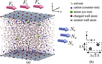
Figure 1: (a) An electrolyte solution between two charged surfaces. (b) A unit cell of the equilateral triangular lattice of the wall atoms in the $x$-$y$ plane.

III Application to aqueous NaCl solution

III.1 Molecular dynamics simulation

We apply the formulation described in the previous section to a system consisting of an aqueous NaCl solution confined between two parallel charged surfaces as shown in Fig. 1. The molecular dynamics simulation method is employed, because it allows an efficient, detailed analysis of the microscopic phenomena at the atomic scale Rotenberg and Pagonabarraga (2013). Each wall consists of a two-dimensional triangular lattice of a model atom, with a lattice spacing $a_{0}=3$ Å. A charged, periodic superstructure with a periodicity $\ell_{c}=3a_{0}$ or $5a_{0}$ is superimposed onto this triangular lattice, so that one atom out of 9 or 25 is negatively charged with one unit charge $-e$. The resulting surface charge density is $\sigma=0.228$ C/m² in the case of $\ell_{c}=3a_{0}$, and $\sigma=0.082$ C/m² in the case of $\ell_{c}=5a_{0}$. The numbers of Na⁺ and Cl^- ions in the electrolyte solution are denoted by $n^{\mathrm{Na}}$ and $n^{\mathrm{Cl}}$, respectively. Then the relation $n^{\mathrm{Na}}=n^{\mathrm{Cl}}+n^{\mathrm{C}}$ holds because of electrical neutrality, where $n^{\mathrm{C}}$ is the number of charged wall atoms. The interactions between water molecules are described by the extended simple point charge (SPC/E) model, and those between ions are described by a sum of electrostatic and Lennard-Jones (LJ) potentials, with parameters taken from Ref. Smith and Dang (1994). The Lorentz–Berthelot mixing rule Allen and Tildesley (1989) is employed for the LJ parameters for water-ion and Na-Cl pairs. For the interaction between a wall atom and a water molecule, a model mimicking a hydrophilic surface at the level of homogeneously distributed hydrogen bond sites is used, where the potential is designed to have orientation dependence reflecting the trend of hydrogen bonds Pertsin and Grunze (2008); Yoshida et al. (2014). The parallel code LAMMPS LAM is used to implement the MD simulation. The number of particles and the volume $V$ are kept constant, and the Nosé–Hoover thermostat is used to maintain the temperature at $T=300$ K (NVT ensemble). Further details of the computational procedure are described in Ref. Yoshida et al. (2014).

Table 1: Transport coefficients in unit $10^{-9}$mol²/Jms; values in parentheses are standard errors for ten simulation runs.

flux\force	$F_{\mathrm{s}}$	$F_{\mathrm{c}}$	$F_{\mathrm{a}}$
$N_{\mathrm{s}}$	$M_{{\mathrm{s}}{\mathrm{s}}}$	$M_{{\mathrm{s}}{\mathrm{c}}}$	$M_{{\mathrm{s}}{\mathrm{a}}}$
	$3754$ ($74$)	$14.51$ ($0.94$)	$10.69$ ($0.40$)
$N_{\mathrm{c}}$	$M_{{\mathrm{c}}{\mathrm{s}}}$	$M_{{\mathrm{c}}{\mathrm{c}}}$	$M_{{\mathrm{c}}{\mathrm{a}}}$
	$14.05$ ($0.99$)	$0.2526$ ($0.0063$)	$0.04447$ ($0.0064$)
$N_{\mathrm{a}}$	$M_{{\mathrm{a}}{\mathrm{s}}}$	$M_{{\mathrm{a}}{\mathrm{c}}}$	$M_{{\mathrm{a}}{\mathrm{a}}}$
	$10.88$ ($0.72$)	$0.04317$ ($0.0069$)	$0.1390$ ($0.0040$)

III.2 Transformation of the generic transport coefficients

We first demonstrate the transformation from the generic transport coefficients $M_{\alpha\beta}$ to the physical parameters $\widetilde{M}_{jk}$. The transport coefficients are evaluated using the Green–Kubo formula (3), for the system of the walls with lateral dimensions of $4.68$ nm $\times 3.6$ nm ($9\times 12$ unit cells, see Fig. 1) and $\sigma=0.228$ C/m² ($\ell_{c}=3a_{0}$), confining $2235$ water molecules, $53$ Na⁺ ions, and $5$ Cl^- ions. The distance between wall atoms determined using the method described in Ref. Yoshida et al. (2014) is $4.12$ nm, and the resulting nominal concentrations of Na⁺ and Cl^- are $1.27$ M and $0.12$ M, respectively. Because of poor statistics in the equilibrium simulations, an extremely long simulation run is required to obtain smooth time-correlation functions in Eq. (3). To circumvent this difficulty, we carry out ten MD simulations with different initial configurations, each of which runs for $5$ ns, and time-integrate the averaged correlation functions.

Table 1 lists the values of $M_{\alpha\beta}$, along with the standard errors for ten simulation runs. Onsager’s reciprocal relations are satisfied reasonably well, which shows the good accuracy of the numerical simulations. Although the bare components of $M_{\alpha\beta}$ are different from the familiar physical parameters, they give some interesting indications. The higher mobility of the excess counter-ions (cations) compensating the negative surfaces charges is indicated by $M_{{\mathrm{c}}{\mathrm{c}}}>M_{{\mathrm{a}}{\mathrm{a}}}$. Regarding cross effects, the clear difference $M_{{\mathrm{s}}{\mathrm{c}}}>M_{{\mathrm{s}}{\mathrm{a}}}$ implies occurrence of the electro-osmotic flow, because the values of $M_{{\mathrm{s}}{\mathrm{c}}}$ and $M_{{\mathrm{s}}{\mathrm{a}}}$ represent the intensity of the solvent flow induced by the force acting on ions.

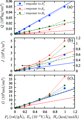
Figure 2: (a) Mass flow density, (b) current density, and (c) diffusion flux density, induced by the pressure gradient, the electric field, and the chemical potential gradient. The linear lines indicate Eq. (6) based on the generic transport coefficients, and the symbols indicate the results of the NEMD simulations with the explicit external fields.

The generic transport coefficients are readily transformed into the physical parameters that are relevant in the situation under which the measurements are performed. Since the most common set of observable quantities for the confined electrolyte solution is $Q$, $J$, and $G$ introduced above, we carry out the NEMD simulations and numerically obtain these fluxes to ensure that the transformation of the transport coefficients works, and to examine the limit of the linear-response assumption. The external forces exerted on $i$th particle in the $x$-direction are $f_{i}^{\mathrm{ext}}=m_{i}P_{x}$ where $P_{x}$ is the mass acceleration simulating the pressure gradient, $f_{i}^{\mathrm{ext}}=q_{i}E_{x}$ where $E_{x}$ is the electric field, and $f_{i}^{\mathrm{ext}}=\psi^{\mathrm{ion}}_{i}H_{x}$ where $H_{x}$ is the force representing the chemical potential gradient of the solute; $m_{i}$ and $q_{i}$ are the mass and charge of $i$th particle, and $\psi^{\mathrm{ion}}_{i}$ is an index of which the value is unity for ions and zero for solvent particles. After an equilibriation for $1$ ns, a production run for $4$ ns is performed at a set of external fields specified, to obtain average values of the mass flow density $Q=(1/V)\sum_{i}m_{i}\dot{x}_{i}$, the electric current density $J=(1/V)\sum_{i}q_{i}\dot{x}_{i}$, and the ion-flux density $G=(1/V)\sum_{i}\psi_{i}^{\mathrm{ion}}\dot{x}_{i}$, which are plotted in Fig. 2. All the fluxes approach asymptotically as $P_{x},E_{x},H_{x}\to 0$, showing that the numerical values of the coefficients in Table 1 correctly reproduce the physical parameters of $\widetilde{M}$ in Eq. (6). The linear-response assumption is valid in the range $P_{x}\leq 0.2$ cal/gÅ, $E_{x}\leq 0.02$ V/Å, and $H_{x}\leq 0.2$ kcal/molÅ. Note that these critical values are extremely large compared with the field strength attainable in laboratories; for instance $P_{x}=0.2$ cal/gÅ along a distance of $1$ $\mu$m results in a pressure difference of $10^{5}$ atm. Figure 2 indicates the linear-response assumption to be valid in quite wide range of the field strengths in the system considered herein.

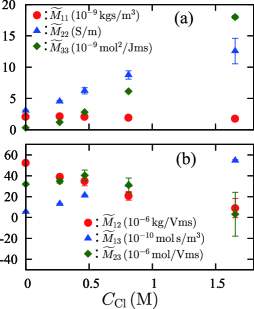
Figure 3: Physical transport coefficients $\widetilde{M}_{jk}$ as functions of the concentration of Cl^- at the midpoint of the channel, in the case of $\sigma=0.082$ C/m². (a) Diagonal components, and (b) off-diagonal components. The error bar indicates the standard errors for ten simulation runs.

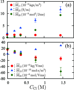
Figure 4: Physical transport coefficients $\widetilde{M}_{jk}$ as functions of the concentration of Cl^-, in the case of $\sigma=0.228$ C/m². See the caption of Fig. 3.

III.3 Influence of salt concentration and flow reversal

At relatively high surface charge densities, the reversal of the electro-osmotic flow, i.e., the negative response of $Q$ to $E_{x}$, can occur as first demonstrated by Qiao and Aluru Qiao and Aluru (2004). Recently we have shown the occurrence of the reversal of the electro-osmotic flow, as well as its reciprocal streaming current, in the linear-response regime Yoshida et al. (2014). In addition to the surface charge density, importance of the concentration of the added salt on the transport properties was also implied in Ref. Yoshida et al. (2014). Here, we examine systematically the influence of the added salt. Specifically, maintaining the surface charge density at $\sigma=0.082$ and $0.228$ C/m², the concentration of the added salt is varied by controlling the number of excess pairs of Na⁺ and Cl^-.

In Figs. 3 and 4, the components of the matrix $\widetilde{M}$ are plotted as functions of the bulk concentration of Cl^-, denoted by $C_{\mathrm{Cl}}$, where $C_{\mathrm{Cl}}$ is measured at the midpoint of the gap. In these parameter ranges, the nominal concentration of Na⁺ ranges from $0.41$ to $1.57$ M in Fig. 3, and it ranges from $1.15$ to $2.30$ M in Fig. 4. The weak dependence of $\widetilde{M}_{11}$ on the salt concentration indicates that the rate of the pressure-driven Poiseuille-type flow is not influenced significantly, implying the weak variation of the kinetic viscosity of the electrolyte solution in this parameter range. The coefficients $\widetilde{M}_{22}$ and $\widetilde{M}_{33}$, corresponding respectively to the electrical conductivity and the salt diffusivity, increase as the salt concentration due to the increase of the carrier, and so does $\widetilde{M}_{13}$. In contrast, $\widetilde{M}_{12}$ and $\widetilde{M}_{23}$ decrease as the salt concentration. Particularly in the case of $\sigma=0.228$ C/m² (Fig. 4(b)), the values of $\widetilde{M}_{12}$ (and $\widetilde{M}_{21}$), and $\widetilde{M}_{23}$ (and $\widetilde{M}_{32}$) become negative for high concentrations ($C_{\mathrm{Cl}}>0.4$ M), meaning that, in addition to the the electro-osmotic flow and the streaming current, the diffusio-osmotic current (response of $J$ to $H_{x}$) and its reciprocal electro-osmotic diffusion (response of $G$ to $E_{x}$) are anomalously reversed. Here, we note that the matrix $\widetilde{M}$ maintains the positive definiteness for all cases. The fluxes obtained via Eq. (6), corresponding to $\widetilde{M}_{12}$, $\widetilde{M}_{21}$, $\widetilde{M}_{23}$, and $\widetilde{M}_{32}$, at $C_{\mathrm{Cl}}=1.44$ M are shown in Fig. 5, along with the results of the NEMD simulations. Although the nonlinear effect at extremely large external fields changes the direction of the fluxes, the results of the NEMD simulations converge to the values predicted by the transport coefficients in the linear-response regime, which confirms the occurrence of the reversed responses.

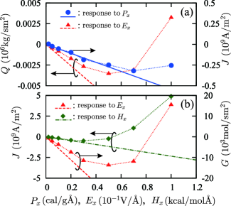
Figure 5: (a) Inverted electro-osmotic flow and the reciprocal streaming current, and (b) inverted electro-osmosis and the reciprocal diffusio-osmotic current, observed at $\sigma=0.228$ C/m² and $C_{\mathrm{Cl}}=1.44$ M. See the caption of Fig. 2.

It was shown in Refs. Qiao and Aluru (2004); Yoshida et al. (2014) that the strong binding or the counter-ion condensation at high surface charge densities makes co-ions gather in the region where the solution can move, which results in the reversed electro-osmotic flow. We show in Fig. 6 the distribution of the net charge across the channel width for several values of the salt concentration in the case of $\sigma=0.228$ C/m². At high salt concentrations, a negatively charged region is observed around $z=9$ Å. The existence of the negative net charge in the mobile region also explains the reversed diffusio-osmotic current and electro-osmotic diffusion. Although the average concentration of the counter-ions compensating the surface charge is large, most of them condense at the charged surface and do not respond to the diffusion force or to the electric field. As a result, the number of co-ions accumulating in the mobile region exceeds that of counter-ions there, which causes diffusio-osmotic current and electro-osmotic diffusion in the direction opposite to the usual ones.

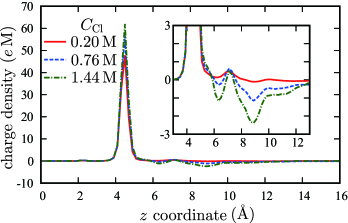
Figure 6: Charge density distributions in the $z$-direction, for the case of $\sigma=0.228$ C/m². The origin of the coordinate is at the position of the wall atoms. The inset is the same data on a smaller scale.

IV Conclusion

We have described the transformation of the generic transport coefficients $M_{\alpha\beta}$ for a confined electrolyte solution into the physical transport coefficients $\widetilde{M}_{jk}$, which preserves Onsager’s reciprocal relation. Applicability of the transformation has been demonstrated by using the equilibrium and NEMD simulations for the system of an aqueous NaCl solution confined in a charged nano-channel. The generic coefficients are obtainable in the standard framework of equilibrium molecular dynamics and Green–Kubo formula, while the physical ones are more naturally obtained using the NEMD simulations in the limit of small external fields. The influence of the salt concentration on the transport coefficients has been investigated at two values of the surface charge densities. Our results are expected to be generic, and provide important information for the design of electrochemical devices using nano-porous media. Furthermore, anomalous reversal of the diffusio-osmotic current, as well as the reversal of the electro-osmotic flow, at high surface charge density and high concentration of added salt, has been shown to occur in the linear-response regime.

The usefulness of the transformation would be more pronounced for complex systems with larger number of chemical components in the solution, because any physical parameters of interest in an experimental setup are immediately obtained via the transformation from the generic transport coefficients, which are evaluated in a straightforward manner simply using the fluxes of each component as shown in Eq. (3). Our future work thus includes application of the presented scheme to different chemical components and to wider parameter ranges, possibly using the coarse-grained molecular simulation (e.g., Ref. Kinjo et al. (2014)), in systems for which the all atom molecular dynamics simulation is not feasible.