Adaptive Augmented Lagrangian Methods:
Algorithms and Practical Numerical Experience—Detailed Version

Abstract

In this paper, we consider augmented Lagrangian (AL) algorithms for solving large-scale nonlinear optimization problems that execute adaptive strategies for updating the penalty parameter. Our work is motivated by the recently proposed adaptive AL trust region method by Curtis, Jiang, and Robinson [Math. Prog., DOI: 10.1007/s10107-014-0784-y, 2013]. The first focal point of this paper is a new variant of the approach that employs a line search rather than a trust region strategy, where a critical algorithmic feature for the line search strategy is the use of convexified piecewise quadratic models of the AL function for computing the search directions. We prove global convergence guarantees for our line search algorithm that are on par with those for the previously proposed trust region method. A second focal point of this paper is the practical performance of the line search and trust region algorithm variants in Matlab software, as well as that of an adaptive penalty parameter updating strategy incorporated into the Lancelot software. We test these methods on problems from the CUTEst and COPS collections, as well as on challenging test problems related to optimal power flow. Our numerical experience suggests that the adaptive algorithms outperform traditional AL methods in terms of efficiency and reliability. As with traditional AL algorithms, the adaptive methods are matrix-free and thus represent a viable option for solving extreme-scale problems.

49M05, 49M15, 49M29, 49M37, 65K05, 65K10, 90C06, 90C30, 93B40

1 Introduction

Augmented Lagrangian (AL) methods [25, 33] have recently regained popularity due to growing interests in solving extreme-scale nonlinear optimization problems. These methods are attractive in such settings as they can be implemented matrix-free [2, 3, 11, 28] and have global and local convergence guarantees under relatively weak assumptions [18, 26]. Furthermore, certain variants of AL methods [20, 21] have proved to be very efficient for solving certain structured problems [6, 34, 36].

A new AL trust region method was recently proposed and analyzed in [15]. The novel feature of that algorithm is an adaptive strategy for updating the penalty parameter inspired by techniques for performing such updates in the context of exact penalty methods [7, 8, 29]. This feature is designed to overcome a potentially serious drawback of traditional AL methods, which is that they may be ineffective during some (early) iterations due to poor choices of the penalty parameter and/or Lagrange multiplier estimates. In such situations, the poor choices of these quantities may lead to little or no improvement in the primal space and, in fact, the iterates may diverge from even a well-chosen initial iterate. The key idea for avoiding this behavior in the algorithm proposed in [15] is to adaptively update the penalty parameter during the step computation in order to ensure that the trial step yields a sufficiently large reduction in linearized constraint violation, thus steering the optimization process steadily toward constraint satisfaction.

The contributions of this paper are two-fold. First, we present an AL line search method based on the same framework employed for the trust region method in [15]. The main difference between our new approach and that in [15], besides the differences inherent in using line searches instead of a trust region strategy, is that we utilize a convexified piecewise quadratic model of the AL function to compute the search direction in each iteration. With this modification, we prove that our line search method achieves global convergence guarantees on par with those proved for the trust region method in [15]. The second contribution of this paper is that we perform extensive numerical experiments with a Matlab implementation of the adaptive algorithms (i.e., both line search and trust region variants) and an implementation of an adaptive penalty parameter updating strategy in the Lancelot software [12]. We test these implementations on problems from the CUTEst [22] and COPS [5] collections, as well as on test problems related to optimal power flow [37]. Our results indicate that our adaptive algorithms outperform traditional AL methods in terms of efficiency and reliability.

The remainder of the paper is organized as follows. In §2, we present our adaptive AL line search method and state convergence results. Details and proofs of these results, which draw from those in [15], can be found in Appendices 5 and 6. We then provide numerical results in §3 to illustrate the effectiveness of our implementations of our adaptive AL algorithms. We give conclusions in §4.

Notation. We often drop function arguments once a function is defined. We also use a subscript on a function name to denote its value corresponding to algorithmic quantities using the same subscript. For example, for a function $f:\mathbb{R}^{n}\to\mathbb{R}$, if $x_{k}$ is the value for the variable $x$ during iteration $k$ of an algorithm, then $f_{k}:=f(x_{k})$. We also often use subscripts for constants to indicate the algorithmic quantity to which they correspond. For example, $\gamma_{\mu}$ denotes a parameter corresponding to the algorithmic quantity $\mu$.

2 An Adaptive Augmented Lagrangian Line Search Algorithm

2.1 Preliminaries

We assume that all problems under our consideration are formulated as

$${\displaystyle\operatorname*{minimize}_{x\in\mathbb{R}^{n}}}\ f(x)\ \operatorname*{subject\;to}\ c(x)=0,\;\;l\leq x\leq u.$$ (1)

Here, we assume that the objective function $f:\mathbb{R}^{n}\to\mathbb{R}$ and constraint function $c:\mathbb{R}^{n}\to\mathbb{R}^{m}$ are twice continuously differentiable, and that the variable lower bound vector $l\in\mathbb{R}^{n}$ and upper bound vector $u\in\mathbb{R}^{n}$ satisfy $l\leq u$. Our goal is to design an algorithm that will compute a first-order primal-dual stationary point for problem (1). However, in order for the algorithm to be suitable as a general-purpose approach, it should have mechanisms for terminating and providing useful information when an instance of (1) is (locally) infeasible. In such cases, we have designed our algorithm so that it transitions to finding an infeasible first-order stationary point for the nonlinear feasibility problem

$${\displaystyle\operatorname*{minimize}_{x\in\mathbb{R}^{n}}}\ v(x)\ \operatorname*{subject\;to}\ l\leq x\leq u,$$ (2)

where $v:\mathbb{R}^{n}\to\mathbb{R}$ is defined as $v(x)={\textstyle\frac{1}{2}}\|c(x)\|_{2}^{2}$.

As implied by the previous paragraph, our algorithm requires first-order stationarity conditions for problems (1) and (2), which can be stated in the following manner. First, introducing a Lagrange multiplier vector $y\in\mathbb{R}^{m}$, we define the Lagrangian for problem (1), call it $\ell:\mathbb{R}^{n}\times\mathbb{R}^{m}\to\mathbb{R}$, by

$$\ell(x,y)=f(x)-c(x)^{T}\!y.$$

Then, defining the gradient of the objective function $g:\mathbb{R}^{n}\to\mathbb{R}^{n}$ by $g(x)=\nabla\!f(x)$, the Jacobian of the constraint functions $J:\mathbb{R}^{n}\to\mathbb{R}^{m\times n}$ by $J(x)=\nabla\!c(x)$, and the projection operator onto the bounds $P:\mathbb{R}^{n}\to\mathbb{R}^{n}$, component-wise for $i\in\{1,\dots,n\}$, by

$$[P(x)]_{i}=\left\{\begin{aligned} &l_{i}&&\text{if }x_{i}\leq l_{i}\\ &u_{i}&&\text{if }x_{i}\geq u_{i}\\ &x_{i}&&\text{otherwise}\end{aligned}\right.$$

we may introduce the primal-dual stationarity measure $F_{\mbox{\tiny L}}:\mathbb{R}^{n}\times\mathbb{R}^{m}\to\mathbb{R}^{n}$ given by

$$F_{\mbox{\tiny L}}(x,y)=P(x-\nabla\!_{x}\ell(x,y))-x=P(x-(g(x)-J(x)^{T}\!y))-x.$$

First-order primal-dual stationary points for (1) can then be characterized as zeros of the primal-dual stationarity measure $F_{\mbox{\tiny OPT}}:\mathbb{R}^{n}\times\mathbb{R}^{m}\to\mathbb{R}^{n+m}$ defined by stacking the stationarity measure $F_{\mbox{\tiny L}}$ and the constraint function $-c$, i.e., a first-order primal-dual stationary point for (1) is any pair $(x,y)$ with $l\leq x\leq u$ satisfying

$$0=F_{\mbox{\tiny OPT}}(x,y)=\begin{pmatrix}F_{\mbox{\tiny L}}(x,y)\\ -c(x)\end{pmatrix}=\begin{pmatrix}P(x-\nabla\!_{x}\ell(x,y))-x\\ \nabla\!_{y}\ell(x,y)\end{pmatrix}.$$ (3)

Similarly, a first-order primal stationary point for (2) is any $x$ with $l\leq x\leq u$ satisfying

$$0=F_{\mbox{\tiny FEAS}}(x),$$ (4)

where $F_{\mbox{\tiny FEAS}}:\mathbb{R}^{n}\to\mathbb{R}^{n}$ is defined by

$$F_{\mbox{\tiny FEAS}}(x)=P(x-\nabla\!_{x}v(x))-x=P(x-J(x)^{T}\!c(x))-x.$$

In particular, if $l\leq x\leq u$, $v(x)>0$, and (4) holds, then $x$ is an infeasible stationary point for problem (1).

Over the past decades, a variety of effective numerical methods have been proposed for solving large-scale bound-constrained optimization problems. Hence, the critical issue in solving problem (1) is how to handle the presence of the equality constraints. As in the wide variety of penalty methods that have been proposed, the strategy adopted by AL methods is to remove these constraints, but push the algorithm to satisfy them through the addition of influential terms in the objective. In this manner, problem (1) (or at least (2)) can be solved via a sequence of bound-constrained subproblems—thus allowing AL methods to exploit the methods that are available for subproblems of this type. Specifically, AL methods consider a sequence of subproblems in which the objective is a weighted sum of the Lagrangian $\ell$ and the constraint violation measure $v$. By scaling $\ell$ by a penalty parameter $\mu\geq 0$, each subproblem involves the minimization of a function ${\mathcal{L}}:\mathbb{R}^{n}\times\mathbb{R}^{m}\times\mathbb{R}\to\mathbb{R}$, called the augmented Lagrangian (AL), defined by

$${\mathcal{L}}(x,y,\mu)=\mu\ell(x,y)+v(x)=\mu(f(x)-c(x)^{T}\!y)+{\textstyle\frac{1}{2}}\|c(x)\|_{2}^{2}.$$

Observe that the gradient of the AL with respect to $x$, evaluated at $(x,y,\mu)$, is given by

$$\nabla\!_{x}{\mathcal{L}}(x,y,\mu)=\mu\big{(}g(x)-J(x)^{T}\!\pi(x,y,\mu)\big{)},$$

where we define the function $\pi:\mathbb{R}^{n}\times\mathbb{R}^{m}\times\mathbb{R}\to\mathbb{R}^{m}$ by

$$\pi(x,y,\mu)=y-\tfrac{1}{\mu}c(x).$$ (5)

Hence, each subproblem to be solved in an AL method has the form

$${\displaystyle\operatorname*{minimize}_{x\in\mathbb{R}^{n}}}\ {\mathcal{L}}(x,y,\mu)\ \operatorname*{subject\;to}\ l\leq x\leq u.$$ (6)

Given a pair $(y,\mu)$, a first-order stationary point for problem (6) is any zero of the primal-dual stationarity measure $F_{\mbox{\tiny AL}}:\mathbb{R}^{n}\times\mathbb{R}^{m}\times\mathbb{R}\to\mathbb{R}^{n}$, defined similarly to $F_{\mbox{\tiny L}}$ but with the Lagrangian replaced by the augmented Lagrangian; i.e., given $(y,\mu)$, a first-order stationary point for (6) is any $x$ satisfying

$$0=F_{\mbox{\tiny AL}}(x,y,\mu)=P(x-\nabla\!_{x}{\mathcal{L}}(x,y,\mu))-x.$$ (7)

Given a pair $(y,\mu)$ with $\mu>0$, a traditional AL method proceeds by (approximately) solving (6), which is to say that it finds a point, call it $x(y,\mu)$, that (approximately) satisfies (7). If the resulting pair $(x(y,\mu),y)$ is not a first-order primal-dual stationary point for (1), then the method would modify the Lagrange multiplier $y$ or penalty parameter $\mu$ so that, hopefully, the solution of the subsequent subproblem (of the form (6)) yields a better primal-dual solution estimate for (1). The function $\pi$ plays a critical role in this procedure. In particular, observe that if $c(x(y,\mu))=0$, then $\pi(x(y,\mu),y,\mu)=y$ and (7) would imply $F_{\mbox{\tiny OPT}}(x(y,\mu),y)=0$, i.e., that $(x(y,\mu),y)$ is a first-order primal-dual stationary point for (1). Hence, if the constraint violation at $x(y,\mu)$ is sufficiently small, then a traditional AL method would set the new value of $y$ as $\pi(x,y,\mu)$. Otherwise, if the constraint violation is not sufficiently small, then the penalty parameter is decreased to place a higher priority on reducing it during subsequent iterations.

2.2 Algorithm Description

Our AL line search algorithm is similar to the AL trust region method proposed in [15], except for two key differences: it executes line searches rather than using a trust region framework, and it employs a convexified piecewise quadratic model of the AL function for computing the search direction in each iteration. The main motivation for utilizing a convexified model is to ensure that each computed search direction is a direction of strict descent for the AL function from the current iterate, which is necessary to ensure the well-posedness of the line search. However, it should be noted that, practically speaking, the convexification of the model does not necessarily add any computational difficulties when computing each direction; see §3.1.1. Similar to the trust region method proposed in [15], a critical component of our algorithm is the adaptive strategy for updating the penalty parameter $\mu$ during the search direction computation. This is used to ensure steady progress—i.e., steer the algorithm—toward solving (1) (or at least (2)) by monitoring predicted improvements in linearized feasibility.

The central component of each iteration of our algorithm is the search direction computation. In our approach, this computation is performed based on local models of the constraint violation measure $v$ and the AL function ${\mathcal{L}}$ at the current iterate, which at iteration $k$ is given by $(x_{k},y_{k},\mu_{k})$. The local models that we employ for these functions are, respectively, $q_{v}:\mathbb{R}^{n}\to\mathbb{R}$ and $\tilde{q}:\mathbb{R}^{n}\to\mathbb{R}$, defined as follows:

$$q_{v}(s;x) ={\textstyle\frac{1}{2}}\|c(x)+J(x)s\|_{2}^{2}$$

$$\tilde{q}(s;x,y,\mu) ={\mathcal{L}}(x,y)+\nabla\!_{x}{\mathcal{L}}(x,y)^{T}\!s+\max\{{\textstyle\frac{1}{2}}s^{T}\!(\mu\nabla\!^{\,2}_{xx}\ell(x,y)+J(x)^{T}\!J(x))s,0\}.$$

We note that $q_{v}$ is a typical Gauss-Newton model of the constraint violation measure $v$, and $\tilde{q}$ is a convexification of a second-order approximation of the augmented Lagrangian. (We use the notation $\tilde{q}$ rather than simply $q$ to distinguish between the model above and the second-order model—without the max—that appears extensively in [15].)

Our algorithm computes two types of steps during each iteration. The purpose of the first step, which we refer to as the steering step, is to gauge the progress towards linearized feasibility that may be achieved (locally) from the current iterate. This is done by (approximately) minimizing our model $q_{v}$ of the constraint violation measure $v$ within the bound constraints and a trust region. Then, a step of the second type is computed by (approximately) minimizing our model $\tilde{q}$ of the AL function ${\mathcal{L}}$ within the bound constraints and a trust region. If the reduction in the model $q_{v}$ yielded by the latter step is sufficiently large—say, compared to that yielded by the steering step—then the algorithm proceeds using this step as the search direction. Otherwise, the penalty parameter may be reduced, in which case a step of the latter type is recomputed. This process repeats iteratively until a search direction is computed that yields a sufficiently large (or at least not too negative) reduction in $q_{v}$. As such, the iterate sequence is intended to make steady progress toward (or at least approximately maintain) constraint satisfaction throughout the optimization process, regardless of the initial penalty parameter value.

We now describe this process in more detail. During iteration $k$, the steering step $r_{k}$ is computed via the optimization subproblem given by

$${\displaystyle\operatorname*{minimize}_{r\in\mathbb{R}^{n}}}\ q_{v}(r;x_{k})\ \operatorname*{subject\;to}\ l\leq x_{k}+r\leq u,\,\|r\|_{2}\leq\theta_{k},$$ (8)

where, for some constant $\delta>0$, the trust region radius is defined to be

$$\theta_{k}:=\delta\|F_{\mbox{\tiny FEAS}}(x_{k})\|_{2}\geq 0.$$ (9)

A consequence of this choice of trust region radius is that it forces the steering step to be smaller in norm as the iterates of the algorithm approach any stationary point of the constraint violation measure [35]. This prevents the steering step from being too large relative to the progress that can be made toward minimizing $v$. While (8) is a convex optimization problem for which there are efficient methods, in order to reduce computational expense our algorithm only requires $r_{k}$ to be an approximate solution of (8). In particular, we merely require that $r_{k}$ yields a reduction in $q_{v}$ that is proportional to that yielded by the associated Cauchy step (see (16a) later on), which is defined to be

$$\overline{r}_{k}:=\overline{r}(x_{k},\theta_{k}):=P(x_{k}-\overline{\beta}_{k}J_{k}^{T}c_{k})-x_{k}$$ (10)

for $\overline{\beta}_{k}:=\overline{\beta}(x_{k},\theta_{k})$ such that, for some $\varepsilon_{r}\in(0,1)$, the step $\overline{r}_{k}$ satisfies

$$\varDelta q_{v}(\overline{r}_{k};x_{k}):=q_{v}(0;x_{k})-q_{v}(\overline{r}_{k};x_{k})\geq-\varepsilon_{r}\overline{r}_{k}^{T}\!J_{k}^{T}\!c_{k}\;\;\text{and}\;\;\|\overline{r}_{k}\|_{2}\leq\theta_{k}.$$ (11)

Appropriate values for $\overline{\beta}_{k}$ and $\overline{r}_{k}$—along with auxiliary nonnegative scalar quantities $\varepsilon_{k}$ and $\Gamma_{k}$ to be used in subsequent calculations in our method—are computed by Algorithm 1. The quantity $\varDelta q_{v}(\overline{r}_{k};x_{k})$ representing the predicted reduction in constraint violation yielded by $\overline{r}_{k}$ is guaranteed to be positive at any $x_{k}$ that is not a first-order stationary point for $v$ subject to the bound constraints; see part (i) of Lemma 5.4. We define a similar reduction $\varDelta q_{v}(r_{k};x_{k})$ for the steering step $r_{k}$.

Algorithm 1 Cauchy step computation for the feasibility subproblem (8)

1:procedure Cauchy_feasibility($x_{k},\theta_{k}$)

2:     restrictions : $\theta_{k}\geq 0$.

3:     available constants : $\{\varepsilon_{r},\gamma\}\subset(0,1)$.

4:     Compute the smallest integer $l_{k}\geq 0$ satisfying $\|P(x_{k}-\gamma^{l_{k}}J_{k}^{T}\!c_{k})-x_{k}\|_{2}\leq\theta_{k}$.

5:     if $l_{k}>0$ then

6:         Set $\Gamma_{k}\leftarrow\min\{2,{\textstyle\frac{1}{2}}(1+\|P(x_{k}-\gamma^{l_{k}-1}J_{k}^{T}\!c_{k})-x_{k}\|_{2}/\theta_{k})\}$.

7:     else

8:         Set $\Gamma_{k}\leftarrow 2$.

9:     end if

10:     Set $\overline{\beta}_{k}\leftarrow\gamma^{l_{k}}$, $\overline{r}_{k}\leftarrow P(x_{k}-\overline{\beta}_{k}J_{k}^{T}\!c_{k})-x_{k}$, and $\varepsilon_{k}\leftarrow 0$.

11:     while $\overline{r}_{k}$ does not satisfy (11) do

12:         Set $\varepsilon_{k}\leftarrow\max(\varepsilon_{k},-\varDelta q_{v}(\overline{r}_{k};x_{k})/\overline{r}_{k}^{T}\!J_{k}^{T}\!c_{k})$.

13:         Set $\overline{\beta}_{k}\leftarrow\gamma\overline{\beta}_{k}$ and $\overline{r}_{k}\leftarrow P(x_{k}-\overline{\beta}_{k}J_{k}^{T}\!c_{k})-x_{k}$.

14:     end while

15:     return : $(\overline{\beta}_{k},\overline{r}_{k},\varepsilon_{k},\Gamma_{k})$

16:end procedure

After computing a steering step $r_{k}$, we proceed to compute a trial step $s_{k}$ via

$${\displaystyle\operatorname*{minimize}_{s\in\mathbb{R}^{n}}}\ \tilde{q}(s;x_{k},y_{k},\mu_{k})\ \operatorname*{subject\;to}\ l\leq x_{k}+s\leq u,\,\|s\|_{2}\leq\Theta_{k},$$ (12)

where, given $\Gamma_{k}>1$ from the output of Algorithm 1, we define the trust region radius

$$\Theta_{k}:=\Theta(x_{k},y_{k},\mu_{k},\Gamma_{k})=\Gamma_{k}\delta\|F_{\mbox{\tiny AL}}(x_{k},y_{k},\mu_{k})\|_{2}\geq 0.$$ (13)

As for the steering step, we allow inexactness in the solution of (12) by only requiring the step $s_{k}$ to satisfy a Cauchy decrease condition (see (16b) later on), where the Cauchy step for problem (12) is

$$\overline{s}_{k}:=\overline{s}(x_{k},y_{k},\mu_{k},\Theta_{k},\varepsilon_{k}):=P(x_{k}-\overline{\alpha}_{k}\nabla\!_{x}{\mathcal{L}}(x_{k},y_{k},\mu_{k}))-x_{k}$$ (14)

for $\overline{\alpha}_{k}=\overline{\alpha}(x_{k},y_{k},\mu_{k},\Theta_{k},\varepsilon_{k})$ such that, for $\varepsilon_{k}\geq 0$ returned from Algorithm 1, $\overline{s}_{k}$ yields

$$\varDelta\tilde{q}(\overline{s}_{k};x_{k},y_{k},\mu_{k}):= \ \tilde{q}(0;x_{k},y_{k},\mu_{k})-\tilde{q}(\overline{s}_{k};x_{k},y_{k},\mu_{k})$$ (15)

$$\geq \ -\frac{(\varepsilon_{k}+\varepsilon_{r})}{2}\overline{s}_{k}^{T}\!\nabla\!_{x}{\mathcal{L}}(x_{k},y_{k},\mu_{k})\;\;\text{and}\;\;\|\overline{s}_{k}\|_{2}\leq\Theta_{k}.$$

Algorithm 2 describes our procedure for computing $\overline{\alpha}_{k}$ and $\overline{s}_{k}$. (The importance of incorporating $\Gamma_{k}$ in (13) and $\varepsilon_{k}$ in (15) is revealed in the proofs of Lemmas 5.2 and 5.3.) The quantity $\varDelta\tilde{q}(\overline{s}_{k};x_{k},y_{k},\mu_{k})$ representing the predicted reduction in ${\mathcal{L}}(\cdot,y_{k},\mu_{k})$ yielded by $\overline{s}_{k}$ is guaranteed to be positive at any $x_{k}$ that is not a first-order stationary point for ${\mathcal{L}}(\cdot,y_{k},\mu_{k})$ subject to the bound constraints; see part (ii) of Lemma 5.4. A similar quantity $\varDelta\tilde{q}(s_{k};x_{k},y_{k},\mu_{k})$ is also used for the search direction $s_{k}$.

Algorithm 2 Cauchy step computation for the Augmented Lagrangian subproblem (12).

1:procedure Cauchy_AL($x_{k},y_{k},\mu_{k},\Theta_{k},\varepsilon_{k}$)

2:     restrictions : $\mu_{k}>0$, $\Theta_{k}>0$, and $\varepsilon_{k}\geq 0$.

3:     available constant : $\gamma\in(0,1)$.

4:     Set $\overline{\alpha}_{k}\leftarrow 1$ and $\overline{s}_{k}\leftarrow P(x_{k}-\overline{\alpha}_{k}\nabla\!_{x}{\mathcal{L}}(x_{k},y_{k},\mu_{k}))-x_{k}$.

5:     while (15) is not satisfied do

6:         Set $\overline{\alpha}_{k}\leftarrow\gamma\overline{\alpha}_{k}$ and $\overline{s}_{k}\leftarrow P(x_{k}-\overline{\alpha}_{k}\nabla\!_{x}{\mathcal{L}}(x_{k},y_{k},\mu_{k}))-x_{k}$.

7:     end while

8:     return : $(\overline{\alpha}_{k},\overline{s}_{k})$

9:end procedure

Our complete algorithm is given as Algorithm 3 on page 3. In particular, the $k$th iteration proceeds as follows. Given the $k$th iterate tuple $(x_{k},y_{k},\mu_{k})$, the algorithm first determines whether the first-order primal-dual stationarity conditions for (1) or the first-order stationarity condition for (2) are satisfied. If either is the case, then the algorithm terminates, but otherwise the method enters the while loop in line 11 to check for stationarity with respect to the AL function. This loop is guaranteed to terminate finitely; see Lemma 5.1. Next, after computing appropriate trust region radii and Cauchy steps, the method enters a block for computing the steering step $r_{k}$ and trial step $s_{k}$. Through the while loop on line 19, the overall goal of this block is to compute (approximate) solutions of subproblems (8) and (12) satisfying

$$\varDelta\tilde{q}(s_{k};x_{k},y_{k},\mu_{k}) \geq\kappa_{1}\varDelta\tilde{q}(\overline{s}_{k};x_{k},y_{k},\mu_{k})>0,\;\;\;l\leq x_{k}+s_{k}\leq u,\;\;\;\|s_{k}\|_{2}\leq\Theta_{k},$$ (16a)

$$\varDelta q_{v}(r_{k};x_{k}) \geq\kappa_{2}\varDelta q_{v}(\overline{r}_{k};x_{k})\geq 0,\;\;\;\qquad\,\hskip 2.84544ptl\leq x_{k}+r_{k}\leq u,\;\;\;\|r_{k}\|_{2}\leq\theta_{k},$$ (16b)

$$\;\;\text{and}\;\;\varDelta q_{v}(s_{k};x_{k}) \geq\min\{\kappa_{3}\varDelta q_{v}(r_{k};x_{k}),v_{k}-{\textstyle\frac{1}{2}}(\kappa_{t}t_{j})^{2}\}.$$ (16c)

In these conditions, the method employs user-provided constants $\{\kappa_{1},\kappa_{2},\kappa_{3},\kappa_{t}\}\subset(0,1)$ and the algorithmic quantity $t_{j}>0$ representing the $j$th constraint violation target. It should be noted that, for sufficiently small $\mu>0$, many approximate solutions to (8) and (12) satisfy (16), but for our purposes (see Theorem 2.2) it is sufficient that, for sufficiently small $\mu>0$, they are at least satisfied by $r_{k}=\overline{r}_{k}$ and $s_{k}=\overline{s}_{k}$. A complete description of the motivations underlying conditions (16) can be found in [15, Section 3]. In short, (16a) and (16b) are Cauchy decrease conditions while (16c) ensures that the trial step predicts progress toward constraint satisfaction, or at least predicts that any increase in constraint violation is limited (when the right-hand side is negative).

Algorithm 3 Adaptive Augmented Lagrangian Line Search Algorithm

1:Choose $\{\gamma,\gamma_{\mu},\gamma_{\alpha},\gamma_{t},\gamma_{T},\kappa_{1},\kappa_{2},\kappa_{3},\varepsilon_{r},\kappa_{t},\eta_{s},\eta_{vs}\}\subset(0,1)$ and $\{\delta,\epsilon,Y\}\subset(0,\infty)$ such that $\eta_{vs}\geq\eta_{s}$.

2:Choose initial primal-dual pair $(x_{0},y_{0})$ and initialize $\{\mu_{0},\delta_{0},t_{0},t_{1},T_{1},Y_{1}\}\subset(0,\infty)$ such that $Y_{1}\geq Y$ and $\|y_{0}\|_{2}\leq Y_{1}$.

3:Set $k\leftarrow 0$, $k_{0}\leftarrow 0$, and $j\leftarrow 1$.

4:loop

5:     if $F_{\mbox{\tiny OPT}}(x_{k},y_{k})=0$, then

6:          return the first-order stationary solution $(x_{k},y_{k})$.

7:     end if

8:     if $\|c_{k}\|_{2}>0$ and $F_{\mbox{\tiny FEAS}}(x_{k})=0$, then

9:          return the infeasible stationary point $x_{k}$.

10:     end if

11:     while $F_{\mbox{\tiny AL}}(x_{k},y_{k},\mu_{k})=0$, do

12:          Set $\mu_{k}\leftarrow\gamma_{\mu}\mu_{k}$.

13:     end while

14:     Define $\theta_{k}$ by (9).

15:     Use Algorithm 1 to compute $(\overline{\beta}_{k},\overline{r}_{k},\varepsilon_{k},\Gamma_{k})=\text{\sc Cauchy\_feasibility}(x_{k},\theta_{k})$.

16:     Define $\Theta_{k}$ by (13).

17:     Use Algorithm 2 to compute $(\overline{\alpha}_{k},\overline{s}_{k})=\text{\sc Cauchy\_AL}(x_{k},y_{k},\mu_{k},\Theta_{k},\varepsilon_{k})$.

18:     Compute approximate solutions $r_{k}$ to (8) and $s_{k}$ to (12) that satisfy (16a)–(16b).

19:     while (16c) is not satisfied or $F_{\mbox{\tiny AL}}(x_{k},y_{k},\mu_{k})=0$, do

20:         Set $\mu_{k}\leftarrow\gamma_{\mu}\mu_{k}$ and define $\Theta_{k}$ by (13).

21:         Use Algorithm 2 to compute $(\overline{\alpha}_{k},\overline{s}_{k})=\text{\sc Cauchy\_AL}(x_{k},y_{k},\mu_{k},\Theta_{k},\varepsilon_{k})$.

22:         Compute an approximate solution $s_{k}$ to (12) satisfying (16a).

23:     end while

24:      Set $\alpha_{k}\leftarrow\gamma_{\alpha}^{l}$ where $l\geq 0$ is the smallest integer satisfying (17).

25:      Set $x_{k+1}\leftarrow x_{k}+\alpha_{k}s_{k}$.

26:     if $\|c_{k+1}\|_{2}\leq t_{j}$, then

27:          Compute any ${\widehat{y\mkern 2.8mu}\mkern-2.8mu}{}_{k+1}$ satisfying (18).

28:         if $\min\{\|F_{\mbox{\tiny L}}(x_{k+1},{\widehat{y\mkern 2.8mu}\mkern-2.8mu}{}_{k+1})\|_{2},\|F_{\mbox{\tiny AL}}(x_{k+1},y_{k},\mu_{k})\|_{2}\}\leq T_{j}$, then

29:               Set $k_{j}\leftarrow k+1$ and $Y_{j+1}\leftarrow\max\{Y,t_{j-1}^{-\epsilon}\}$.

30:               Set $t_{j+1}\leftarrow\min\{\gamma_{t}t_{j},t_{j}^{1+\epsilon}\}$ and $T_{j+1}\leftarrow\gamma_{T}T_{j}$.

31:              Set $y_{k+1}$ from (19) where $\alpha_{y}$ satisfies (20).

32:              Set $j\leftarrow j+1$.

33:         else

34:              Set $y_{k+1}\leftarrow y_{k}$.

35:         end if

36:     else

37:         Set $y_{k+1}\leftarrow y_{k}$.

38:     end if

39:     Set $\mu_{k+1}\leftarrow\mu_{k}$.

40:     Set $k\leftarrow k+1$.

41:end loop

With the search direction $s_{k}$ in hand, the method proceeds to perform a backtracking line search along the strict descent direction $s_{k}$ for ${\mathcal{L}}(\cdot,y_{k},\mu_{k})$ at $x_{k}$. Specifically, for a given $\gamma_{\alpha}\in(0,1)$, the method computes the smallest integer $l\geq 0$ such that

$${\mathcal{L}}(x_{k}+\gamma_{\alpha}^{l}s_{k},y_{k},\mu_{k})\leq{\mathcal{L}}(x_{k},y_{k},\mu_{k})-\eta_{s}\gamma_{\alpha}^{l}\varDelta\widetilde{q}(s_{k};x_{k},y_{k},\mu_{k}),$$ (17)

and then sets $\alpha_{k}\leftarrow\gamma_{\alpha}^{l}$ and $x_{k+1}\leftarrow x_{k}+\alpha_{k}s_{k}$. The remainder of the iteration is then composed of potential modifications of the Lagrange multiplier vector and target values for the accuracies in minimizing the constraint violation measure and AL function subject to the bound constraints. First, the method checks whether the constraint violation at the next primal iterate $x_{k+1}$ is sufficiently small compared to the target $t_{j}>0$. If this requirement is met, then a multiplier vector ${\widehat{y\mkern 2.8mu}\mkern-2.8mu}{}_{k+1}$ that satisfies

$$\|F_{\mbox{\tiny L}}(x_{k+1},{\widehat{y\mkern 2.8mu}\mkern-2.8mu}{}_{k+1})\|_{2}\leq\min\left\{\|F_{\mbox{\tiny L}}(x_{k+1},y_{k})\|_{2},\|F_{\mbox{\tiny L}}(x_{k+1},\pi(x_{k+1},y_{k},\mu_{k}))\|_{2}\right\}$$ (18)

is computed. Two obvious potential choices for ${\widehat{y\mkern 2.8mu}\mkern-2.8mu}{}_{k+1}$ are $y_{k}$ and $\pi(x_{k+1},y_{k},\mu_{k})$, but another viable candidate would be an approximate least-squares multiplier estimate (which may be computed via a linearly constrained optimization subproblem). The method then checks if either $\|F_{\mbox{\tiny L}}(x_{k+1},{\widehat{y\mkern 2.8mu}\mkern-2.8mu}{}_{k+1})\|_{2}$ or $\|F_{\mbox{\tiny AL}}(x_{k+1},y_{k},\mu_{k})\|_{2}$ is sufficiently small with respect to the target value $T_{j}>0$. If so, then new target values $t_{j+1}<t_{j}$ and $T_{j+1}<T_{j}$ are set, $Y_{j+1}\geq Y_{j}$ is chosen, and a new Lagrange multiplier vector is set as

$$y_{k+1}\leftarrow(1-\alpha_{y})y_{k}+\alpha_{y}{\widehat{y\mkern 2.8mu}\mkern-2.8mu}{}_{k+1},$$ (19)

where $\alpha_{y}$ is the largest value in $[0,1]$ such that

$$\|(1-\alpha_{y})y_{k}+\alpha_{y}{\widehat{y\mkern 2.8mu}\mkern-2.8mu}{}_{k+1}\|_{2}\leq Y_{j+1}.$$ (20)

This updating procedure is well-defined since the choice $\alpha_{y}\leftarrow 0$ results in $y_{k+1}\leftarrow y_{k}$, for which (20) is satisfied since $\|y_{k}\|_{2}\leq Y_{j}\leq Y_{j+1}$. If either line 26 or line 28 in Algorithm 3 tests false, then the method simply sets $y_{k+1}\leftarrow y_{k}$. We note that unlike more traditional augmented Lagrangian approaches [2, 11], the penalty parameter is not adjusted on the basis of a test like that on line 26, but instead relies on our steering procedure. Moreover, in our approach we decrease the target values at a linear rate for simplicity, but more sophisticated approaches may be used [11].

2.3 Well-posedness and global convergence

In this section, we state two vital results, namely that Algorithm 3 is well posed, and that limit points of the iterate sequence have desirable properties. Proofs of these results, which are similar to those in [15], are given in Appendices A and B. In order to show well-posedness of the algorithm, we make the following formal assumption.

Assumption 2.1.

At each given $x_{k}$, the objective function $f$ and constraint function $c$ are both twice-continuously differentiable.

Under this assumption, we have the following theorem.

Theorem 2.2.

Suppose that Assumption 2.1 holds. Then the $k$th iteration of Algorithm 3 is well posed. That is, either the algorithm will terminate in line 6 or 9, or it will compute $\mu_{k}>0$ such that $F_{\mbox{\tiny AL}}(x_{k},y_{k},\mu_{k})\neq 0$ and for the steps $s_{k}=\overline{s}_{k}$ and $r_{k}=\overline{r}_{k}$ the conditions in (16) will be satisfied, in which case $(x_{k+1},y_{k+1},\mu_{k+1})$ will be computed.

According to Theorem 2.2, we have that Algorithm 3 will either terminate finitely or produce an infinite sequence of iterates. If it terminates finitely—which can only occur if line 6 or 9 is executed—then the algorithm has computed a first-order stationary solution or an infeasible stationary point and there is nothing else to prove about the algorithm’s performance in such cases. Therefore, it remains to focus on the global convergence properties of Algorithm 3 under the assumption that the sequence $\{(x_{k},y_{k},\mu_{k})\}$ is infinite. For such cases, we make the following additional assumption.

Assumption 2.3.

The primal sequences $\{x_{k}\}$ and $\{x_{k}+s_{k}\}$ are contained in a convex compact set over which the objective function $f$ and constraint function $c$ are both twice-continuously differentiable.

Our main global convergence result for Algorithm 3 is as follows.

Theorem 2.4.

Suppose that Assumptions 2.2 and 2.3 hold. Then one of the following must hold:

• every limit point $x_{*}$ of $\{x_{k}\}$ is an infeasible stationary point;

• $\mu_{k}\nrightarrow 0$ and there exists an infinite ordered set ${\mathcal{K}}\subseteq\mathbb{N}$ such that every limit point of $\{(x_{k},{\widehat{y\mkern 2.8mu}\mkern-2.8mu}{}_{k})\}_{k\in{\mathcal{K}}}$ is first-order stationary for (1); or

• $\mu_{k}\to 0$, every limit point of $\{x_{k}\}$ is feasible, and if there exists a positive integer $p$ such that $\mu_{k_{j}-1}\geq\gamma_{\mu}^{p}\mu_{k_{j-1}-1}$ for all sufficiently large $j$, then there exists an infinite ordered set ${\mathcal{J}}\subseteq\mathbb{N}$ such that any limit point of either $\{(x_{k_{j}},{\widehat{y\mkern 2.8mu}\mkern-2.8mu}{}_{k_{j}})\}_{j\in{\mathcal{J}}}$ or $\{(x_{k_{j}},y_{k_{j}-1})\}_{j\in{\mathcal{J}}}$ is first-order stationary for (1).

Observe that the conclusions are exactly the same as in [15, Theorem 3.14]. We also call the readers attention to the comments following [15, Theorem 3.14], which discuss the consequences of these results. In particular, these comments suggest how Algorithm 3 may be modified to guarantee convergence to first-order stationary points, even in case (iii) of the theorem. However, as mentioned in [15], we do not consider these modifications to the algorithm to have practical benefits. This perspective is supported by the numerical tests presented in the following section.

3 Numerical Experiments

In this section, we provide evidence that steering can have a positive effect on the performance of AL algorithms. To best illustrate the influence of steering, we implemented and tested algorithms in two pieces of software. First, in Matlab, we implemented our adaptive AL line search algorithm, i.e., Algorithm 3, and the adaptive AL trust region method given as [15, Algorithm 4]. Since these methods were implemented from scratch, we had control over every aspect of the code, which allowed us to implement all features described in this paper and in [15]. Second, we implemented a simple modification of the AL trust region algorithm in the Lancelot software package [12]. Our only modification to Lancelot was to incorporate a basic form of steering; i.e., we did not change other aspects of Lancelot, such as the mechanisms for triggering a multiplier update. In this manner, we were also able to isolate the effect that steering had on numerical performance, though it should be noted that there were differences between Algorithm 3 and our implemented algorithm in Lancelot in terms of, e.g., the multiplier updates.

While we provide an extensive amount of information about the results of our experiments in this section, further information can be found in Appendix 7.

3.1 Matlab implementation

3.1.1 Implementation details

Our Matlab software was comprised of six algorithm variants. The algorithms were implemented as part of the same package so that most of the algorithmic components were exactly the same; the primary differences related to the step acceptance mechanisms and the manner in which the Lagrange multiplier estimates and penalty parameter were updated. First, for comparison against algorithms that utilized our steering mechanism, we implemented line search and trust region variants of a basic augmented Lagrangian method, given as [15, Algorithm 1]. We refer to these algorithms as BAL-LS (basic augmented Lagrangian, line search) and BAL-TR (trust region), respectively. These algorithms clearly differed in that one used a line search and the other used a trust region strategy for step acceptance, but the other difference was that, like Algorithm 3 in this paper, BAL-LS employed a convexified model of the AL function. (We discuss more details about the use of this convexified model below.) The other algorithms implemented in our software included two variants of Algorithm 3 and two variants of [15, Algorithm 4]. The first variants of each, which we refer to as AAL-LS and AAL-TR (adaptive, as opposed to basic), were straightforward implementations of these algorithms, whereas the latter variants, which we refer to as AAL-LS-safe and AAL-TR-safe, included an implementation of a safeguarding procedure for the steering mechanism. The safeguarding procedure will be described in detail shortly.

The main per-iteration computational expense for each algorithm variant can be attributed to the search direction computations. For computing a search direction via an approximate solve of (12) or [15, Prob. (3.8)], all algorithms essentially used the same procedure. For simplicity, all algorithms considered variants of these subproblems in which the $\ell_{2}$-norm trust region was replaced by an $\ell_{\infty}$-norm trust region so that the subproblems were bound-constrained. (The same modification was used in the Cauchy step calculations.) Then, starting with the Cauchy step as the initial solution estimate and defining the initial working set by the bounds identified as active by the Cauchy step, a projected conjugate gradient (PCG) method was used to compute an improved solution. During the PCG routine, if a new trial solution violated a bound constraint that was not already part of the working set, then this bound was added to the working set and the PCG routine was reinitialized. By contrast, if the reduced subproblem (corresponding to the current working set) was solved sufficiently accurately, then a check for termination was performed. In particular, multiplier estimates were computed for the working set elements. If these multiplier estimates were all nonnegative (or at least larger than a small negative number), then the subproblem was deemed to be solved and the routine terminated. Otherwise, an element corresponding to the most negative multiplier estimate was removed from the working set and the PCG routine was reinitialized. We do not claim that the precise manner in which we implemented this approach guaranteed convergence to an exact solution of the subproblem. However, the approach just described was based on well-established methods for solving bound-constrained quadratic optimization problems (QPs), and we found that it worked very well in our experiments. It should be noted that if, at any time, negative curvature was encountered in the PCG routine, then the solver terminated with the current PCG iterate. In this manner, the solutions were generally less accurate when negative curvature was encountered, but we claim that this did not have too adverse an effect on the performance of any of the algorithms.

A few additional comments are necessary to describe our search direction computation procedures. First, it should be noted that for the line search algorithms, the Cauchy step calculation in Algorithm 2 was performed with (15) as stated (i.e., with $\tilde{q}$), but the above PCG routine to compute the search direction was applied to (12) without the convexification for the quadratic term. However, we claim that this choice remains consistent with the stated algorithms since, for all algorithm variants, we performed a sanity check after the computation of the search direction. In particular, the reduction in the model of the AL function yielded by the search direction was compared against that yielded by the corresponding Cauchy step. If the Cauchy step actually provided a better reduction in the model, then the computed search direction was replaced by the Cauchy step. In this sanity check for the line search algorithms, we computed the model reductions with the convexification of the quadratic term (i.e., with $\tilde{q}$), which implies that, overall, our implemented algorithm guaranteed Cauchy decrease in the appropriate model for all algorithms. Second, we remark that for the algorithms that employed a steering mechanism, we did not employ the same procedure to approximately solve (8) or [15, Prob. (3.4)]. Instead, we simply used the Cauchy steps as approximate solutions of these subproblems. Finally, we note that in the steering mechanism, we checked condition (16c) with the Cauchy steps for each subproblem, despite the fact that the search direction was computed as a more accurate solution of (12) or [15, Prob. (3.8)]. This had the effect that the algorithms were able to modify the penalty parameter via the steering mechanism prior to computing the search direction; only Cauchy steps for the subproblems were needed for steering.

Most of the other algorithmic components were implemented similarly to the algorithm in [15]. As an example, for the computation of the estimates $\{\widehat{y}_{k+1}\}$ (which are required to satisfy (18)), we checked whether $\|F_{\mbox{\tiny L}}(x_{k+1},\pi(x_{k+1},y_{k},\mu_{k}))\|_{2}\leq\|F_{\mbox{\tiny L}}(x_{k+1},y_{k})\|_{2}$; if so, then we set $\widehat{y}_{k+1}\leftarrow\pi(x_{k+1},y_{k},\mu_{k})$, and otherwise we set $\widehat{y}_{k+1}\leftarrow y_{k}$. Furthermore, for prescribed tolerances $\{\kappa_{\mbox{\tiny opt}},\kappa_{\mbox{\tiny feas}},\mu_{\mbox{\tiny min}}\}\subset(0,\infty)$, we terminated an algorithm with a declaration that a stationary point was found if

$$\|F_{\mbox{\tiny L}}(x_{k},y_{k})\|_{\infty}\leq\kappa_{\mbox{\tiny opt}}\ \ \text{and}\ \ \|c_{k}\|_{\infty}\leq\kappa_{\mbox{\tiny feas}},$$ (21)

and terminated with a declaration that an infeasible stationary point was found if

$$\|F_{\mbox{\tiny FEAS}}(x_{k})\|_{\infty}\leq\kappa_{\mbox{\tiny opt}},\ \ \|c_{k}\|_{\infty}>\kappa_{\mbox{\tiny feas}},\ \ \text{and}\ \ \mu_{k}\leq\mu_{\mbox{\tiny min}}.$$ (22)

As in [15], this latter set of conditions shows that we did not declare that an infeasible stationary point was found unless the penalty parameter had already been reduced below a prescribed tolerance. This helps in avoiding premature termination when the algorithm could otherwise continue and potentially find a point satisfying (21), which was always the preferred outcome. Each algorithm terminated with a message of failure if neither (21) nor (22) was satisfied within $k_{\mbox{\tiny max}}$ iterations. It should also be noted that the problems were pre-scaled so that the $\ell_{\infty}$-norms of the gradients of the problem functions at the initial point would be less than or equal to a prescribed constant $G>0$. The values for all of these parameters, as well as other input parameter required in the code, are summarized in Table 1. (Values for parameters related to updating the trust region radii required by [15, Algorithm 4] were set as in [15].)

Table 1: Input parameter values used in our Matlab software.

Parameter	Value	Parameter	Value	Parameter	Value	Parameter	Value
$\gamma$	$0.5$	$\kappa_{2}$	$1$	$\eta_{vs}$	$0.9$	$\mu_{\mbox{\tiny min}}$	$10^{-8}$
$\gamma_{\mu}$	$0.1$	$\kappa_{3}$	$10^{-4}$	$\epsilon$	$0.5$	$k_{\mbox{\tiny max}}$	$10^{4}$
$\gamma_{t}$	$0.1$	$\varepsilon_{r}$	$10^{-4}$	$\mu_{0}$	$1$	$G$	$10^{2}$
$\gamma_{T}$	$0.1$	$\kappa_{t}$	$0.9$	$\kappa_{\mbox{\tiny opt}}$	$10^{-5}$
$\kappa_{1}$	$1$	$\eta_{s}$	$10^{-4}$	$\kappa_{\mbox{\tiny feas}}$	$10^{-5}$

We close this subsection with a discussion of some additional differences between the algorithms as stated in this paper and in [15] and those implemented in our software. We claim that none of these differences represents a significant departure from the stated algorithms; we merely made some adjustments to simplify the implementation and to incorporate features that we found to work well in our experiments. First, while all algorithms use the input parameter $\gamma_{\mu}$ given in Table 1 for decreasing the penalty parameter, we decrease the penalty parameter less significantly in the steering mechanism. In particular, in line 20 of Algorithm 3 and line 20 of [15, Algorithm 4], we replace $\gamma_{\mu}$ with $0.7$. Second, in the line search algorithms, rather than set the trust region radii as in (9) and (13) where $\delta$ appears as a constant value, we defined a dynamic sequence, call it $\{\delta_{k}\}$, that depended on the step-size sequence $\{\alpha_{k}\}$. In this manner, $\delta_{k}$ replaced $\delta$ in (9) and (13) for all $k$. We initialized $\delta_{0}\leftarrow 1$. Then, for all $k$, if $\alpha_{k}=1$, then we set $\delta_{k+1}\leftarrow\tfrac{5}{3}\delta_{k}$, and if $\alpha_{k}<1$, then we set $\delta_{k+1}\leftarrow\tfrac{1}{2}\delta_{k}$. Third, to simplify our implementation, we effectively ignored the imposed bounds on the multiplier estimates by setting $Y\leftarrow\infty$ and $Y_{1}\leftarrow\infty$. This choice implies that we always chose $\alpha_{y}\leftarrow 1$ in (19). Fourth, we initialized the target values as

$$t_{1} \leftarrow\max\{10^{2},\min\{10^{4},\|c_{k}\|_{\infty}\}\}$$ (23)

$$\;\;\text{and}\;\;T_{1} \leftarrow\max\{10^{0},\min\{10^{2},\|F_{\mbox{\tiny L}}(x_{k},y_{k})\|_{\infty}\}\}.$$ (24)

Finally, in AAL-LS-safe and AAL-TR-safe, we safeguard the steering procedure by shutting it off whenever the penalty parameter was smaller than a prescribed tolerance. Specifically, we considered the while condition in line 19 of Algorithm 3 and line 19 of [15, Algorithm 4] to be satisfied whenever $\mu_{k}\leq 10^{-4}$.

3.1.2 Results on CUTEst test problems

We tested our Matlab algorithms on the subset of problems from the CUTEst [24] collection that have at least one general constraint and at most $1000$ variables and $1000$ constraints. This set contains $383$ test problems. However, the results that we present in this section are only for those problems for which at least one of our six solvers obtained a successful result, i.e., where (21) or (22) was satisfied. This led to a set of $323$ problems that are represented in the numerical results in this section.

To illustrate the performance of our Matlab software, we use performance profiles as introduced by Dolan and Moré [17] to provide a visual comparison of different measures of performance. Consider a performance profile that measures performance in terms of required iterations until termination. For such a profile, if the graph associated with an algorithm passes through the point $(\alpha,0.\beta)$, then, on $\beta\%$ of the problems, the number of iterations required by the algorithm was less than $2^{\alpha}$ times the number of iterations required by the algorithm that required the fewest number of iterations. At the extremes of the graph, an algorithm with a higher value on the vertical axis may be considered a more efficient algorithm, whereas an algorithm on top at the far right of the graph may be considered more reliable. Since, for most problems, comparing values in the performance profiles for large values of $\alpha$ is not enlightening, we truncated the horizontal axis at 16 and simply remark on the numbers of failures for each algorithm.

Figures 2 and 2 show the results for the three line search variants, namely BAL-LS, AAL-LS, and AAL-LS-safe. The numbers of failures for these algorithms were 25, 3, and 16, respectively. The same conclusion may be drawn from both profiles: the steering variants (with and without safeguarding) were both more efficient and more reliable than the basic algorithm, where efficiency is measured by either the number of iterations (Figure 2) or the number of function evaluations (Figure 2) required. We display the profile for the number of function evaluations required since, for a line search algorithm, this value is always at least as large as the number of iterations, and will be strictly greater whenever backtracking is required to satisfy (17) (yielding $\alpha_{k}<1$). From these profiles, one may observe that unrestricted steering (in AAL-LS) yielded superior performance to restricted steering (in AAL-LS-safe) in terms of both efficiency and reliability; this suggests that safeguarding the steering mechanism may diminish its potential benefits.

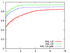
Figure 1: Performance profile for iterations: line search algorithms on the CUTEst set.

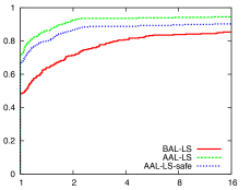
Figure 2: Performance profile for function evaluations: line search algorithms on the CUTEst set.

Figures 4 and 4 show the results for the three trust region variants, namely BAL-TR, AAL-TR, and AAL-TR-safe, the numbers of failures for which were 30, 12, and 20, respectively. Again, as for the line search algorithms, the same conclusion may be drawn from both profiles: the steering variants (with and without safeguarding) are both more efficient and more reliable than the basic algorithm, where now we measure efficiency by either the number of iterations (Figure 4) or the number of gradient evaluations (Figure 4) required before termination. We observe the number of gradient evaluations here (as opposed to the number of function evaluations) since, for a trust region algorithm, this value is never larger than the number of iterations, and will be strictly smaller whenever a step is rejected and the trust-region radius is decreased because of insufficient decrease in the AL function. These profiles also support the other observation that was made by the results for our line search algorithms, i.e., that unrestricted steering may be superior to restricted steering in terms of efficiency and reliability.

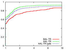
Figure 3: Performance profile for iterations: trust region algorithms on the CUTEst set.

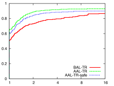
Figure 4: Performance profile for gradient evaluations: trust region algorithms on the CUTEst set.

The performance profiles in Figures 2–4 suggest that steering has practical benefits, and that safeguarding the procedure may limit its potential benefits. However, to be more confident in these claims, one should observe the final penalty parameter values typically produced by the algorithms. These observations are important since one may be concerned whether the algorithms that employ steering yield final penalty parameter values that are often significantly smaller than those yielded by basic AL algorithms. To investigate this possibility in our experiments, we collected the final penalty parameter values produced by all six algorithms; the results are in Table 2. The column titled $\mu_{\mbox{\tiny final}}$ gives a range for the final value of the penalty parameter. (For example, the value 27 in the BAL-LS column indicates that the final penalty parameter value computed by our basic line search AL algorithm fell in the range $[10^{-2},10^{-1})$ for 27 of the problems.)

Table 2: Numbers of CUTEst problems for which the final penalty parameter values were in the given ranges.

$\mu_{\mbox{\tiny final}}$	BAL-LS	AAL-LS	AAL-LS-safe	BAL-TR	AAL-TR	AAL-TR-safe
$1$	139	87	87	156	90	90
$[10^{-1},1)$	43	33	33	35	46	46
$[10^{-2},10^{-1})$	27	37	37	28	29	29
$[10^{-3},10^{-2})$	17	42	42	19	49	49
$[10^{-4},10^{-3})$	22	36	36	18	29	29
$[10^{-5},10^{-4})$	19	28	42	19	25	39
$[10^{-6},10^{-5})$	15	19	11	9	11	9
$(0,10^{-6})$	46	46	40	44	49	37

We remark on two observations about the data in Table 2. First, as may be expected, the algorithms that employ steering typically reduce the penalty parameter below its initial value on some problems on which the other algorithms do not reduce it at all. This, in itself, is not a major concern, since a reasonable reduction in the penalty parameter may cause an algorithm to locate a stationary point more quickly. Second, we remark that the number of problems for which the final penalty parameter was very small (say, less than $10^{-4}$) was similar for all algorithms, even those that employed steering. This suggests that while steering was able to aid in guiding the algorithms toward constraint satisfaction, the algorithms did not reduce the value to such a small value that feasibility became the only priority. Overall, our conclusion from Table 2 is that steering typically decreases the penalty parameter more than does a traditonal updating scheme, but one should not expect that the final penalty parameter value will be reduced unnecessarily small due to steering; rather, steering can have the intended benefit of improving efficiency and reliability by guiding a method toward constraint satisfaction more quickly.

3.1.3 Results on COPS test problems

We also tested our Matlab software on the large-scale constrained problems available in the COPS [5] collection. This test set was designed to provide difficult test cases for nonlinear optimization software; the problems include examples from fluid dynamics, population dynamics, optimal design, mesh smoothing, and optimal control. For our purposes, we solved the smallest versions of the AMPL models [1, 19] provided in the collection. All of our solvers failed to solve the problems named chain, dirichlet, henon, lane_emden, and robot1, so these problems were excluded. The remaining set consisted of the following 17 problems: bearing, camshape, catmix, channel, elec, gasoil, glider, marine, methanol, minsurf, pinene, polygon, rocket, steering, tetra, torsion, and triangle. Since the size of this test set is relatively small, we have decided to display pair-wise comparisons of algorithms in the manner suggested in [30]. That is, for a performance measure of interest (e.g., number of iterations required until termination), we compare solvers, call them $A$ and $B$, on problem $j$ with the logarithmic outperforming factor

$$r^{j}_{AB}:=-\log_{2}({\textrm{m}_{A}^{j}}/{\textrm{m}_{B}^{j}}),\ \ \text{where}\ \ \begin{cases}\textrm{m}_{A}^{j}&\text{is the measure for $A$ on problem $j$}\\ \textrm{m}_{B}^{j}&\text{is the measure for $B$ on problem $j$.}\end{cases}$$ (25)

Therefore, if the measure of interest is iterations required, then $r^{j}_{AB}=p$ would indicate that solver $A$ required $2^{-p}$ the iterations required by solver $B$. For all plots, we focus our attention on the range $p\in[-2,2]$.

The results of our experiments are given in Figures 6–8. For the same reasons as discussed in §3.1.2, we display results for iterations and function evaluations for the line search algorithms, and display results for iterations and gradient evaluations for the trust region algorithms. In addition, here we ignore the results for AAL-LS-safe and AAL-TR-safe since, as in the results in §3.1.2, we did not see benefits in safeguarding the steering mechanism. In each figure, a positive (negative) bar indicates that the algorithm whose name appears above (below) the horizontal axis yielded a better value for the measure on a particular problem. The results are displayed according to the order of the problems listed in the previous paragraph. In Figures 6 and 6 for the line search algorithms, the red bars for problems catmix and polygon indicate that AAL-LS failed on the former and BAL-LS failed on the latter; similarly, in Figures 8 and 8 for the trust region algorithms, the red bar for catmix indicates that AAL-TR failed on it.

The results in Figures 6 and 6 indicate that AAL-LS more often outperforms BAL-LS in terms of iterations and functions evaluations, though the advantage is not overwhelming. On the other hand, it is clear from Figures 8 and 8 that, despite the one failure, AAL-TR is generally superior to BAL-TR. We conclude from these results that steering was beneficial on this test set, especially in terms of the trust region methods.

Figure 5: Outperforming factors for iterations: line search algorithms on the COPS set.

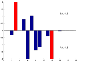
Figure 6: Outperforming factors for function evaluations: line search algorithms on the COPS set.

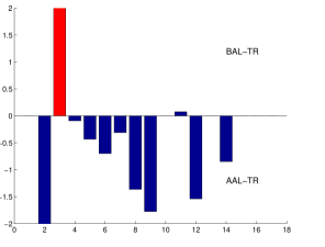
Figure 7: Outperforming factors for iterations: trust region algorithms on the COPS set.

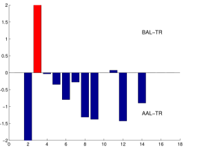
Figure 8: Outperforming factors for gradient evaluations: trust region algorithms on the COPS set.

3.1.4 Results on optimal power flow (OPF) test problems

As a third and final set of experiments for our Matlab software, we tested our algorithms on a collection of optimal power flow (OPF) problems modeled in AMPL using data sets obtained from MATPOWER [37]. OPF problems represent a challenging set of nonconvex problems. The active and reactive power flow and the network balance equations give rise to equality constraints involving nonconvex functions while the inequality constraints are linear and result from placing operating limits on quantities such as flows, voltages, and various control variables. The control variables include the voltages at generator buses and the active-power output of the generating units. The state variables consist of the voltage magnitudes and angles at each node as well as reactive and active flows in each link. Our test set was comprised of $28$ problems modeled on systems having 14 to 662 nodes from the IEEE test set. In particular, there are seven IEEE systems, each modeled in four different ways: (i) in Cartesian coordinates; (ii) in polar coordinates; (iii) with basic approximations to the sin and cos functions in the problem functions; and (iv) with linearized constraints based on DC power flow equations (in place of AC power flow). It should be noted that while linearizing the constraints in formulation (iv) led to a set of linear optimization problems, we still find it interesting to investigate the possible effect that steering may have in this context. All of the test problems were solved by all of our algorithm variants.

We provide outperforming factors in the same manner as in §3.1.3. Figures 10 and 10 reveal that AAL-LS typically outperforms BAL-LS in terms of both iterations and function evaluations, and Figures 12 and 12 reveal that AAL-TR more often than not outperforms BAL-TR in terms of iterations and gradient evaluations. Interestingly, these results suggest more benefits for steering in the line search algorithm than in the trust region algorithm, which is the opposite of that suggested by the results in §3.1.3. However, in any case, we believe that we have presented convincing numerical evidence that steering often has an overall beneficial effect on the performance of our Matlab solvers.

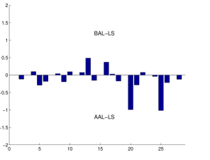
Figure 9: Outperforming factors for iterations: line search algorithms on OPF tests.

Figure 10: Outperforming factors for function evaluations: line search algorithms on OPF tests.

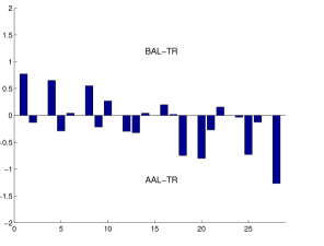
Figure 11: Outperforming factors for iterations: trust region algorithms on OPF tests.

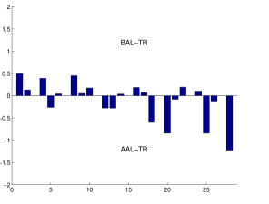
Figure 12: Outperforming factors for gradient evaluations: trust region algorithms on OPF tests.

3.2 An implementation of Lancelot that uses steering

3.2.1 Implementation details

The results for our Matlab software in the previous section illustrate that our adaptive line search AL algorithm and the adaptive trust region AL algorithm from [15] are often more efficient and reliable than basic AL algorithms that employ traditional penalty parameter and Lagrange multiplier updates. Recall, however, that our adaptive methods are different from their basic counterparts in two key ways. First, the steering conditions (16) are used to dynamically decrease the penalty parameter during the optimization process for the AL function. Second, our mechanisms for updating the Lagrange multiplier estimate are different than the basic algorithm outlined in [15, Algorithm 1] since they use optimality measures for both the Lagrangian and the AL functions (see line 28 of Algorithm 3) rather than only that for the AL function. We believe this strategy is more adaptive since it allows for updates to the Lagrange multipliers when the primal estimate is still far from a first-order stationary point for the AL function subject to the bounds.

In this section, we isolate the effect of the first of these differences by incorporating a steering strategy in the Lancelot [12, 13] package that is available in the Galahad library [23]. Specifically, we made three principle enhancements in Lancelot. First, along the lines of the model $q$ in [15] and the convexified model $\tilde{q}$ defined in this paper, we defined the model $\hat{q}:\mathbb{R}^{n}\to\mathbb{R}$ of the AL function given by

$$\hat{q}(s;x,y,\mu)=s^{T}\nabla_{x}\ell\big{(}x,y+c(x)/\mu\big{)}+{\textstyle\frac{1}{2}}s^{T}\big{(}\nabla_{xx}\ell(x,y)+J(x)^{T}\!J(x)/\mu\big{)}s$$

as an alternative to the Newton model $q_{\mbox{\tiny N}}:\mathbb{R}^{n}\to\mathbb{R}$, originally used in Lancelot,

$$q_{\mbox{\tiny N}}(s;x,y,\mu)=s^{T}\nabla_{x}\ell(x,y+c(x)/\mu)+{\textstyle\frac{1}{2}}s^{T}(\nabla_{xx}\ell(x,y+c(x)/\mu)+J(x)^{T}J(x)/\mu)s.$$

As in our adaptive algorithms, the purpose of employing such a model was to ensure that $\hat{q}\to q_{v}$ (pointwise) as $\mu\to 0$, which was required to ensure that our steering procedure was well-defined; see (26a). Second, we added routines to compute generalized Cauchy points [9] for both the constraint violation measure model $q_{v}$ and $\hat{q}$ during the loop in which $\mu$ was decreased until the steering test (16c) was satisfied; recall the while loop starting on line 19 of Algorithm 3. Third, we used the value for $\mu$ determined in the steering procedure to compute a generalized Cauchy point for the Newton model $q_{\mbox{\tiny N}}$, which was the model employed to compute the search direction. For each of the models just discussed, the generalized Cauchy point was computed using either an efficient sequential search along the piece-wise Cauchy arc [10] or via a backtracking Armijo search along the same arc [31]. We remark that this third enhancement would not have been needed if the model $\hat{q}$ were used to compute the search directions. However, in our experiments, it was revealed that using the Newton model typically led to better performance, so the results in this section were obtained using this third enhancement. In our implementation, the user was allowed to control which model was used via control parameters. We also added control parameters that allowed the user to restrict the number of times that the penalty parameter may be reduced in the steering procedure in a given iteration, and that disabled steering once the penalty parameter was reduced below a given tolerance (as in the safeguarding procedure implemented in our Matlab software).

The new package was tested with three different control parameter settings. We refer to algorithm with the first setting, which did not allow any steering to occur, simply as lancelot. The second setting allowed steering to be used initially, but turned it off whenever $\mu\leq 10^{-4}$ (as in our safeguarded Matlab algorithms). We refer to this variant as lancelot-steering-safe. The third setting allowed for steering to be used without any safeguards or restrictions; we refer to this variant as lancelot-steering. As in our Matlab software, the penalty parameter was decreased by a factor of $0.7$ until the steering test (16c) was satisfied. All other control parameters were set to their default lancelot values. The new package will be re-branded as Lancelot in the next official release, Galahad 2.6.

Galahad was compiled with gfortran-4.7 with optimization -O and using Intel MKL BLAS. The code was executed on a single core of an Intel Xeon E5620 (2.4GHz) CPU with 23.5 GiB of RAM.

3.2.2 Results on CUTEst test problems

We tested lancelot, lancelot-steering, and lancelot-steering-safe on the subset of CUTEst problems that have at least one general constraint and at most $10,\!000$ variables and $10,\!000$ constraints. This amounted to $457$ test problems. The results are displayed as performance profiles in Figures 14 and 14, which were created from the 364 of these problems that were solved by at least one of the algorithms. As in the previous sections, since the algorithms are trust region methods, we use the number of iterations and gradient evaluations required as the performance measures of interest.

We can make two important observations from these profiles. First, it is clear that lancelot-steering and lancelot-steering-safe yielded similar performance in terms of iterations and gradient evaluations, which suggests that safeguarding the steering mechanism is not necessary in practice. Second, lancelot-steering and lancelot-steering-safe were both more efficient and reliable than lancelot on these tests, thus showing the positive influence that steering can have on performance.

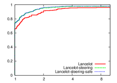
Figure 13: Performance profile for iterations: Lancelot algorithms on the CUTEst set.

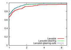
Figure 14: Performance profile for gradient evaluations: Lancelot algorithms on the CUTEst set.

As in §3.1.2, it is important to observe the final penalty parameter values yielded by lancelot-steering and lancelot-steering-safe as opposed to those yielded by lancelot. For these experiments, we collected this information; see Table 3.

Table 3: Numbers of CUTEst problems for which the final penalty parameter values were in the given ranges.

$\mu_{\mbox{\tiny final}}$	lancelot	lancelot-steering	lancelot-steering-safe
$1$	14	1	1
$[10^{-1},1)$	77	1	1
$[10^{-2},10^{-1})$	47	93	93
$[10^{-3},10^{-2})$	27	45	45
$[10^{-4},10^{-3})$	18	28	28
$[10^{-5},10^{-4})$	15	22	22
$[10^{-6},10^{-5})$	12	21	14
$(0,10^{-6})$	19	18	25

We make a few remarks about the results in Table 3. First, as may have been expected, the lancelot-steering and lancelot-steering-safe algorithms typically reduced the penalty parameter below its initial value, even when lancelot did not reduce it at all throughout an entire run. Second, the number of problems for which the final penalty parameter was less than $10^{-4}$ was $171$ for lancelot and $168$ for lancelot-steering. Combining this fact with the previous observation leads us to conclude that steering tended to reduce the penalty parameter from its initial value of $1$, but, overall, it did not decrease it much more aggressively than lancelot. Third, it is interesting to compare the final penalty parameter values for lancelot-steering and lancelot-steering-safe. Of course, these values were equal in any run in which the final penalty parameter was greater than or equal to $10^{-4}$, since this was the threshold value below which safeguarding was activated. Interestingly, however, lancelot-steering-safe actually produced smaller values of the penalty parameter compared to lancelot-steering when the final penalty parameter was smaller than $10^{-4}$. We initially found this observation to be somewhat counterintuitive, but we believe that it can be explained by observing the penalty parameter updating strategy used by lancelot. (Recall that once safeguarding was activated in lancelot-steering-safe, the updating strategy became the same used in lancelot.) In particular, the decrease factor for the penalty parameter used in lancelot is $0.1$, whereas the decrease factor used in steering the penalty parameter was $0.7$. Thus, we believe that lancelot-steering reduced the penalty parameter more gradually once it was reduced below $10^{-4}$ while lancelot-steering-safe could only reduce it in the typical aggressive manner. (We remark that to (potentially) circumvent this inefficiency in lancelot, one could implement a different strategy in which the penalty parameter decrease factor is increased as the penalty parameter decreases, but in a manner that still ensures that the penalty parameter converges to zero when infinitely many decreases occur.) Overall, our conclusion from Table 3 is that steering typically decreases the penalty parameter more than a traditional updating scheme, but the difference is relatively small and we have implemented steering in a way that improves the overall efficiency and reliability of the method.

4 Conclusion

In this paper, we explored the numerical performance of adaptive updates to the Lagrange multiplier vector and penalty parameter in AL methods. Specific to the penalty parameter updating scheme is the use of steering conditions that guide the iterates toward the feasible region and toward dual feasibility in a balanced manner. Similar conditions were first introduced in [8] for exact penalty functions, but have been adapted in [15] and this paper to be appropriate for AL-based methods. Specifically, since AL methods are not exact (in that, in general, the trial steps do not satisfy linearized feasibility for any positive value of the penalty parameter), we allowed for a relaxation of the linearized constraints. This relaxation was based on obtaining a target level of infeasibility that is driven to zero at a modest, but acceptable, rate. This approach is in the spirit of AL algorithms since feasibility and linearized feasibility are only obtained in the limit. It should be noted that, like other AL algorithms, our adaptive methods can be implemented matrix-free, i.e., they only require matrix-vector products. This is of particular importance when solving large problems that have sparse derivative matrices.

As with steering strategies designed for exact penalty functions, our steering conditions proved to yield more efficient and reliable algorithms than a traditional updating strategy. This conclusion was made by performing a variety of numerical tests that involved our own Matlab implementations and a simple modification of the well-known AL software Lancelot. To test the potential for the penalty parameter to be reduced too quickly, we also implemented safeguarded variants of our steering algorithms. Across the board, our results indicate that safeguarding was not necessary and would typically degrade performance when compared to the unrestricted steering approach. We feel confident that these tests clearly show that although our theoretical global convergence guarantee is weaker than some algorithms (i.e., we cannot prove that the penalty parameter will remain bounded under a suitable constraint qualification), this should not be a concern in practice. Finally, we suspect that the steering strategies described in this paper would also likely improve the performance of other AL-based methods such as [4, 27].

Acknowledgments. We would like to thank Sven Leyffer and Victor Zavala from the Argonne National Laboratory for providing us with the AMPL [1, 19] files required to test the optimal power flow problems described in §3.1.4.

5 Well-posedness

Our goal in this appendix is to prove that Algorithm 3 is well-posed under Assumption 2.1. Since this assumption is assumed to hold throughout the remainder of this appendix, we do not refer to it explicitly in the statement of each lemma and proof.

5.1 Preliminary results

Our proof of the well-posedness of Algorithm 3 relies on showing that it will either terminate finitely or will produce an infinite sequence of iterates $\{(x_{k},y_{k},\mu_{k})\}$. In order to show this, we first require that the while loop that begins at line 11 of Algorithm 3 terminates finitely. Since the same loop appears in the AL trust region method in [15] and the proof of the result in the case of that algorithm is the same as that for Algorithm 3, we need only refer to the result in [15] in order to state the following lemma for Algorithm 3.

Lemma 5.1 ([15, Lemma 3.2]).

If line 11 is reached, then $F_{\mbox{\tiny AL}}(x_{k},y_{k},\mu)\neq 0$ for all sufficiently small $\mu>0$.

Next, since the Cauchy steps employed in Algorithm 3 are similar to those employed in the method in [15], we may state the following lemma showing that Algorithms 1 and 2 are well defined when called in lines 15, 17, and 21 of Algorithm 3. It should be noted that a slight difference between Algorithm 2 and the similar procedure in [15] is the use of the convexified model $\tilde{q}$ in (15). However, we claim that this difference does not affect the veracity of the result.

Lemma 5.2 ([15, Lemma 3.3]).

The following hold true:

• The computation of $(\overline{\beta}_{k},\overline{r}_{k},\varepsilon_{k},\Gamma_{k})$ in line 15 is well defined and yields $\Gamma_{k}\in(1,2]$ and $\varepsilon_{k}\in[0,\varepsilon_{r})$.

• The computation of $(\overline{\alpha}_{k},\overline{s}_{k})$ in lines 17 and 21 is well defined.

The next result, similar to [15, Lemma 3.4], highlights critical relationships between $q_{v}$ and $\tilde{q}$ as $\mu\to 0$. Indeed, much of the proof follows exactly the same logic as [15, Lemma 3.4], but we provide a complete proof to account for our present use of the convexified model $\tilde{q}$ and the differences in the trust region radii for the subproblems employed in the algorithms. This result is crucial for showing that the steering condition (16c) is satisfied for all sufficient small $\mu$ (see Lemma 5.5).

Lemma 5.3.

Let $(\overline{\beta}_{k},\overline{r}_{k},\varepsilon_{k},\Gamma_{k})\leftarrow\text{\sc Cauchy\_feasibility}(x_{k},\theta_{k})$ with $\theta_{k}$ defined by (9) and, as quantities dependent on the penalty parameter $\mu>0$, let $(\overline{\alpha}_{k}(\mu),\overline{s}_{k}(\mu))\leftarrow\text{\sc Cauchy\_AL}(x_{k},y_{k},\mu,\Theta_{k}(\mu),\varepsilon_{k})$ with $\Theta_{k}(\mu):=\Gamma_{k}\delta\|F_{\mbox{\tiny AL}}(x_{k},y_{k},\mu)\|_{2}$ (see (13)). Then, the following hold true:

$$\lim_{\mu\to 0}\left(\max_{\|s\|_{2}\leq 2\theta_{k}}|\tilde{q}(s;x_{k},y_{k},\mu)-q_{v}(s;x_{k})|\right) =0,$$ (26a)

$$\lim_{\mu\to 0}\nabla\!_{x}{\mathcal{L}}(x_{k},y_{k},\mu) =J_{k}^{T}c_{k},$$ (26b)

$$\lim_{\mu\to 0}\overline{s}_{k}(\mu) =\overline{r}_{k},$$ (26c)

$$\;\;\text{and}\;\;\lim_{\mu\to 0}\varDelta q_{v}(\overline{s}_{k}(\mu);x_{k}) =\varDelta q_{v}(\overline{r}_{k};x_{k}).$$ (26d)

Proof.

Since $x_{k}$ and $y_{k}$ are fixed during iteration $k$, for ease of exposition we often drop these quantities from function dependencies for the purposes of this proof. From the definitions of $q_{v}$ and $\tilde{q}$, it follows that for some constants $M_{1}>0$ and $M_{2}>0$ independent of $\mu$ we have

$$\max_{\|s\|_{2}\leq 2\theta_{k}}|\tilde{q}(s;\mu)-q_{v}(s)| =\max_{\|s\|_{2}\leq 2\theta_{k}}|\mu\ell_{k}+\mu\nabla\!_{x}\ell_{k}^{T}\!s+\max\{\tfrac{\mu}{2}s^{T}\!\nabla\!_{xx}\ell_{k}s,-{\textstyle\frac{1}{2}}\|J_{k}s\|_{2}^{2}\}|$$

$$\leq\mu M_{1}+\max\{\mu M_{2},-{\textstyle\frac{1}{2}}\|J_{k}s\|_{2}^{2}\}.$$

Since the right-hand side of this expression vanishes as $\mu\to 0$, we have (26a). Further,

$$\nabla\!_{x}{\mathcal{L}}(x_{k},y_{k},\mu)-J_{k}^{T}c_{k}=\mu(g_{k}-J_{k}^{T}y_{k}),$$

which implies that (26b) holds.

We now show that (26c) holds. Our proof considers two cases depending on the value $F_{\mbox{\tiny FEAS}}(x_{k})$. Throughout consideration of these cases, it should be observed that all quantities in Algorithm 1 are unaffected by $\mu$, so they can be considered as fixed quantities.

1. If $F_{\mbox{\tiny FEAS}}(x_{k})=0$, then $\theta_{k}=\delta\|F_{\mbox{\tiny FEAS}}(x_{k})\|_{2}=0$, from which it follows that $\overline{r}_{k}=0$ and $\varDelta q_{v}(\overline{r}_{k})=0$. Furthermore, from (26b), we have $\Theta_{k}(\mu)\to 0$ as $\mu\to 0$, which means $\overline{s}_{k}(\mu)\to 0=\overline{r}_{k}$, as desired.

2. Now suppose that $F_{\mbox{\tiny FEAS}}(x_{k})\neq 0$. In the following arguments, we define the following functions of a nonnegative integer $l$ and positive scalar $\mu$:

   $$r_{k}(l)=P(x_{k}-\gamma^{l}J_{k}^{T}\!c_{k})-x_{k}\quad\text{and}\quad s_{k}(l,\mu)=P(x_{k}-\gamma^{l}\nabla\!_{x}{\mathcal{L}}(\mu))-x_{k}.$$

   We also define $l_{\beta}\geq 0$ to be the integer such that $\overline{\beta}_{k}=\gamma^{l_{\beta}}$ (see Algorithm 1), which implies that

   $$\overline{r}_{k}=r_{k}(l_{\beta}).$$ (27)

   We have as a consequence of (26b) that

   $$\lim_{\mu\to 0}s_{k}(l,\mu)=r_{k}(l)\;\;\text{for any}\;\;l\geq 0.$$

   In particular, this implies with (27) that

   $$\lim_{\mu\to 0}s_{k}(l_{\beta},\mu)=r_{k}(l_{\beta})=\overline{r}_{k}.$$ (28)

   Thus, (26c) follows as long as

   $$\overline{s}_{k}(\mu)=s_{k}(l_{\beta},\mu)\quad\text{for all sufficiently small}\quad\mu>0.$$ (29)

   Since the computation of $\overline{s}_{k}(\mu)$ (via the Cauchy_AL routine stated as Algorithm 2) computes a nonnegative integer $l_{\alpha,\mu}$ such that

   $$\overline{s}_{k}(\mu)=P(x_{k}-\gamma^{l_{\alpha,\mu}}\nabla\!_{x}{\mathcal{L}}(\mu))-x_{k},$$

   it follows that (29) can be proved by showing that $l_{\alpha,\mu}=l_{\beta}$ for all sufficiently small $\mu>0$. As a preliminary result in the proof of this fact, we first show that for $l_{k}$ computed in Algorithm 1 we have

   $$\min\{l_{\beta},l_{\alpha,\mu}\}\geq l_{k}\quad\text{for all sufficiently small}\quad\mu>0.$$ (30)

   Indeed, if $l_{k}=0$, then (30) holds trivially. Thus, let us suppose that $l_{k}>0$. According to the procedures in Algorithm 1, it is clear that $l_{\beta}\geq l_{k}$. Hence, we may turn our attention to $l_{\alpha,\mu}$. From the definition of $\Theta_{k}(\mu)$ (in the statement of this lemma), (26b), the manner in which $\Gamma_{k}$ is set in Algorithm 1, the fact that $\theta_{k}>0$, and since $\|P(x_{k}-\gamma^{l_{k}-1}J_{k}^{T}\!c_{k})-x_{k}\|_{2}>\theta_{k}$ due to the manner in which $l_{k}$ is set in Algorithm 1, we have that

   $$\lim_{\mu\to 0}\Theta_{k}(\mu) =\lim_{\mu\to 0}\Gamma_{k}\delta\|F_{\mbox{\tiny AL}}(x_{k},y_{k},\mu)\|_{2}=\Gamma_{k}\delta\|F_{\mbox{\tiny FEAS}}(x_{k})\|_{2}=\Gamma_{k}\theta_{k}$$

   $$=\min\left\{2,{\textstyle\frac{1}{2}}\left(1+\frac{\|P(x_{k}-\gamma^{l_{k}-1}J_{k}^{T}\!c_{k})-x_{k}\|_{2}}{\theta_{k}}\right)\right\}\theta_{k}$$

   $$=\min\left\{2\theta_{k},{\textstyle\frac{1}{2}}\left(\theta_{k}+\|P(x_{k}-\gamma^{l_{k}-1}J_{k}^{T}\!c_{k})-x_{k}\|_{2}\right)\right\}$$

   $$\in\big{(}\theta_{k},\|P(x_{k}-\gamma^{l_{k}-1}J_{k}^{T}\!c_{k})-x_{k}\|_{2}\big{)}.$$

   Along with (26b), this implies that for all sufficiently small $\mu>0$ we have

   $$\lim_{\mu\to 0}\|P(x_{k}-\gamma^{l_{k}-1}\nabla\!_{x}{\mathcal{L}}(\mu))-x_{k}\|_{2}=\|P(x_{k}-\gamma^{l_{k}-1}J_{k}^{T}\!c_{k})-x_{k}\|_{2}>\Theta_{k}(\mu).$$

   This shows that $l_{\alpha,\mu}\geq l_{k}$ holds for all sufficiently small $\mu>0$. Consequently, we have (30).

   Having ensured that (30) holds, we proceed to prove that $l_{\alpha,\mu}=l_{\beta}$ for all sufficiently small $\mu>0$. It follows from the definition of $l_{\beta}$, (27), the procedures of Algorithm 1 (e.g., the manner in which $\varepsilon_{k}$ is set), and part (i) of Lemma 5.2 that

   $$-\frac{\varDelta q_{v}(\overline{r}_{k})}{\overline{r}_{k}^{T}\!J_{k}^{T}\!c_{k}}=-\frac{\varDelta q_{v}\big{(}r_{k}(l_{\beta})\big{)}}{r_{k}(l_{\beta})^{T}\!J_{k}^{T}\!c_{k}} \geq\epsilon_{r}$$ (31)

   $$\quad\text{and}\quad-\frac{\varDelta q_{v}\big{(}r_{k}(l)\big{)}}{r_{k}(l)^{T}\!J_{k}^{T}\!c_{k}}\leq\epsilon_{k} <\epsilon_{r}\;\;\text{for all integers $l_{k}\leq l<l_{\beta}$.}\;\;$$

   (Here, it is important to note that [14, Theorem 12.1.4] can be invoked to ensure that all denominators in (31) are negative.) It follows from (26b), (28), (26a), (31), and part (i) of Lemma 5.2 that

   $$\lim_{\mu\to 0}-\frac{\varDelta\tilde{q}\big{(}s_{k}(l_{\beta},\mu)\big{)}}{s_{k}(l_{\beta},\mu)^{T}\nabla\!_{x}{\mathcal{L}}(\mu)}=-\frac{\varDelta q_{v}(\overline{r}_{k})}{\overline{r}_{k}^{T}\!J_{k}^{T}\!c_{k}}\geq\varepsilon_{r}>\frac{\varepsilon_{k}+\varepsilon_{r}}{2}$$ (32)

   and

   $$\lim_{\mu\to 0}-\frac{\varDelta\tilde{q}\big{(}s_{k}(l,\mu)\big{)}}{s_{k}(l,\mu)^{T}\nabla\!_{x}{\mathcal{L}}(\mu)}=-\frac{\varDelta q_{v}\big{(}r_{k}(l)\big{)}}{r_{k}(l)^{T}\!J_{k}^{T}\!c_{k}}\leq\varepsilon_{k}<\frac{\varepsilon_{k}+\varepsilon_{r}}{2}\quad\text{for all integers $l_{k}\leq l<l_{\beta}$.}\quad$$ (33)

   It now follows from (30), (32), (33), and (15) that $l_{\alpha,\mu}=l_{\beta}$ for all sufficiently small $\mu>0$. As previously mentioned, this proves (26c).

Finally, we notice that (26d) follows from (26c) and continuity of the model $q_{v}$. ∎

We also need the following lemma related to Cauchy decreases in the models $q_{v}$ and $\tilde{q}$. The conclusions of the lemma are similar to [15, Lemma 3.5], but here we account for the convexified model $\tilde{q}$ and other differences in the subproblems employed here as opposed to those in [15].

Lemma 5.4.

Let $\Omega$ be any scalar value such that

$$\Omega\geq\max\{\|\mu_{k}\nabla\!^{\,2}_{xx}\ell(x_{k},y_{k})+J_{k}^{T}\!J_{k}\|_{2},\|J_{k}^{T}\!J_{k}\|_{2}\}.$$ (34)

Then, the following hold true:

• For some $\kappa_{4}\in(0,1)$, the Cauchy step for subproblem (8) yields

  $$\varDelta q_{v}(\overline{r}_{k};x_{k})\geq\kappa_{4}\|F_{\mbox{\tiny FEAS}}(x_{k})\|_{2}^{2}\min\left\{\delta,\frac{1}{1+\Omega}\right\}.$$ (35)

• For some $\kappa_{5}\in(0,1)$, the Cauchy step for subproblem (12) yields

  $$\varDelta\tilde{q}(\overline{s}_{k};x_{k},y_{k},\mu_{k})\geq\kappa_{5}\|F_{\mbox{\tiny AL}}(x_{k},y_{k},\mu_{k})\|_{2}^{2}\min\left\{\delta,\frac{1}{1+\Omega}\right\}.$$ (36)

Proof.

Let $\Sigma_{k}:=1+\sup\{|\omega_{k}(r)|:0<\|r\|_{2}\leq\theta_{k}\}$, where

$$\omega_{k}(r)=\frac{-\varDelta q_{v}(r;x_{k})-r^{T}\!J_{k}^{T}\!c_{k}}{\|r\|_{2}^{2}}\;\;\text{for all}\;\;r\in\mathbb{R}^{n}.$$

In fact, using (34), the Cauchy-Schwartz inequality, and standard norm inequalities, we have that

$$\omega_{k}(r)=\frac{r^{T}\!J_{k}^{T}\!J_{k}r}{2\|r\|_{2}^{2}}\leq\Omega\;\;\text{for all}\;\;r\in\mathbb{R}^{n}.$$

Hence, $\Sigma_{k}\leq 1+\Omega$. The requirement (11) and [32, Theorem 4.4] then yield, for some $\bar{\kappa}_{4}\in(0,1)$, that

$$\varDelta q_{v}(\overline{r}_{k};x_{k})\geq\epsilon_{r}\bar{\kappa}_{4}\|F_{\mbox{\tiny FEAS}}(x_{k})\|_{2}\min\left\{\theta_{k},\frac{1}{\Sigma_{k}}\|F_{\mbox{\tiny FEAS}}(x_{k})\|_{2}\right\}.$$

which, with (9), implies that (35) follows with $\kappa_{4}:=\epsilon_{r}\bar{\kappa}_{4}$.

We now show (36) in a similar manner. Let $\bar{\Sigma}_{k}:=1+\sup\{|\bar{\omega}_{k}(s)|:0<\|s\|_{2}\leq\Theta_{k}\}$ where

$$\bar{\omega}_{k}(s):=\frac{-\varDelta\tilde{q}(s;x_{k},y_{k},\mu_{k})-s^{T}\!\nabla\!_{x}{\mathcal{L}}(x_{k},y_{k},\mu_{k})}{\|s\|_{2}^{2}}\;\;\text{for all}\;\;s\in\mathbb{R}^{n}.$$

Using (34), we have in a similar manner as above that

$$\bar{\omega}_{k}(s) =\frac{\max\{\mu_{k}s^{T}\!\nabla\!^{\,2}_{xx}\ell(x_{k},y_{k},\mu_{k})s+s^{T}\!J_{k}^{T}\!J_{k}s,0\}}{2\|s\|_{2}^{2}}$$

$$\leq\frac{\|\mu_{k}\nabla\!^{\,2}_{xx}\ell(x_{k},y_{k},\mu_{k})+J_{k}^{T}\!J_{k}\|_{2}\|s\|_{2}^{2}}{2\|s\|_{2}^{2}}\leq\Omega.$$

Thus, $\bar{\Sigma}_{k}\leq 1+\Omega$. The requirement (15) and [32, Theorem 4.4] then yield, for some $\bar{\kappa}_{5}\in(0,1)$, that

$$\varDelta\tilde{q}(\overline{s}_{k};x_{k},y_{k},\mu_{k})\geq\frac{\epsilon_{k}+\epsilon_{r}}{2}\bar{\kappa}_{5}\|F_{\mbox{\tiny AL}}(x_{k},y_{k},\mu_{k})\|_{2}\min\left\{\Theta_{k},\frac{1}{\bar{\Sigma}_{k}}\|F_{\mbox{\tiny AL}}(x_{k},y_{k},\mu_{k})\|_{2}\right\},$$

which, with (13) and Lemma 5.2(i), implies that (36) follows with $\kappa_{5}:=\tfrac{1}{2}\epsilon_{r}\bar{\kappa}_{5}$. ∎

The next lemma shows that the while loop at line 19, which is responsible for ensuring that our adaptive steering conditions in (16) are satisfied, terminates finitely. The proof of this is similar to the second part of [15, Theorem 3.6]

Lemma 5.5.

The while loop that begins at line 19 of Algorithm 3 terminates finitely.

Proof.

Since Lemma 5.1 ensures that the latter condition in the while loop is satisfied for all sufficiently small $\mu_{k}>0$, it suffices to show that $s_{k}=\overline{s}_{k}$ and $r_{k}=\overline{r}_{k}$ satisfy (16c) for all sufficiently small $\mu_{k}>0$. To see this, we may borrow notation from Lemma 5.3—i.e., to consider $s_{k}=\overline{s}_{k}$ as a quantity dependent on a parameter $\mu>0$—and observe that (26d) implies

$$\lim_{\mu\to 0}\varDelta q_{v}(s_{k}(\mu);x_{k})=\lim_{\mu\to 0}\varDelta q_{v}(\overline{s}_{k}(\mu);x_{k})=\varDelta q_{v}(\overline{r}_{k};x_{k})=\varDelta q_{v}(r_{k};x_{k}).$$ (37)

If $\varDelta q_{v}(r_{k};x_{k})>0$, then (37) implies that (16c) is satisfied for sufficiently small $\mu_{k}>0$. Otherwise,

$$\varDelta q_{v}(r_{k};x_{k})=\varDelta q_{v}(\overline{r}_{k};x_{k})=0,$$ (38)

which along with (35) implies that $F_{\mbox{\tiny FEAS}}(x_{k})=0$. We may now consider two cases depending on whether $x_{k}$ is feasible for (1). If $c_{k}\neq 0$, then Algorithm 3 would have terminated in line 9, meaning that the while loop at line 19 would not have been reached. On the other hand, if $c_{k}=0$, then (38) implies

$$\min\{\kappa_{3}\varDelta q_{v}(r_{k};x_{k}),v_{k}-{\textstyle\frac{1}{2}}(\kappa_{t}t_{j})^{2}\}=-{\textstyle\frac{1}{2}}(\kappa_{t}t_{j})^{2}<0.$$ (39)

This last strict inequality follows since $t_{j}>0$ by construction and $\kappa_{t}\in(0,1)$ by choice. Therefore, we can deduce that (16c) will be satisfied for sufficiently small $\mu_{k}>0$ by observing (37), (38) and (39). ∎

The final lemma of this section shows that $s_{k}$ is a strict descent direction for the AL function. The conclusion of this lemma is the primary motivation for our use of the convexified model $\tilde{q}$.

Lemma 5.6.

At line 24 of Algorithm 3, the search direction $s_{k}$ is a strict descent direction for ${\mathcal{L}}(\cdot,y_{k},\mu_{k})$ from $x_{k}$. In particular,

$$\nabla\!_{x}{\mathcal{L}}(x_{k},y_{k},\mu_{k})^{T}s_{k}\leq-\varDelta\tilde{q}(s_{k};x_{k},y_{k},\mu_{k})\leq-\kappa_{1}\varDelta\tilde{q}(\overline{s}_{k};x_{k},y_{k},\mu_{k})<0.$$ (40)

Proof.

From the definition of $\tilde{q}$, we find

$$\varDelta\tilde{q}(s_{k};x_{k},y_{k},\mu_{k}) =\tilde{q}(0;x_{k},y_{k},\mu_{k})-\tilde{q}(s_{k};x_{k},y_{k},\mu_{k})$$

$$=-\nabla\!_{x}{\mathcal{L}}(x_{k},y_{k},\mu_{k})^{T}\!s_{k}-\max\{{\textstyle\frac{1}{2}}s_{k}^{T}\!(\mu_{k}\nabla\!^{\,2}_{xx}\ell(x_{k},y_{k})+J_{k}^{T}J_{k})s_{k},0\}$$

$$\leq-\nabla\!_{x}{\mathcal{L}}(x_{k},y_{k},\mu_{k})^{T}\!s_{k}.$$

It follows from this inequality and (16a) that

$$\nabla\!_{x}{\mathcal{L}}(x_{k},y_{k},\mu_{k})^{T}\!s_{k}\leq-\varDelta\tilde{q}(s_{k};x_{k},y_{k},\mu_{k})\leq-\kappa_{1}\varDelta\tilde{q}(\overline{s}_{k};x_{k},y_{k},\mu_{k})<0,$$

as desired. ∎

5.2 Proof of well-posedness result

Proof of Theorem 2.2.

If, during the $k$th iteration, Algorithm 3 terminates in line 6 or 9, then there is nothing to prove. Thus, to proceed in the proof, we may assume that line 11 is reached. Lemma 5.1 then ensures that

$$F_{\mbox{\tiny AL}}(x_{k},y_{k},\mu)\neq 0\;\;\text{for all sufficiently small}\;\;\mu>0.$$ (41)

Consequently, the while loop in line 11 will terminate for a sufficiently small $\mu_{k}>0$. Next, by construction, conditions (16a) and (16b) are satisfied for any $\mu_{k}>0$ by $s_{k}=\overline{s}_{k}$ and $r_{k}=\overline{r}_{k}$. Lemma 5.5 then shows that for a sufficiently small $\mu_{k}>0$, (16c) is also satisfied by $s_{k}=\overline{s}_{k}$ and $r_{k}=\overline{r}_{k}$. Therefore, line 24 will be reached. Finally, Lemma 5.6 ensures that $\alpha_{k}$ in line 24 is well-defined. This completes the proof as all remaining lines in the $k$th iteration are explicit. ∎

6 Global Convergence

We shall tacitly presume that Assumption 2.3 holds throughout this section, and not state it explicitly. This assumption and the bound on the multipliers enforced in line 31 of Algorithm 3 imply that there exists a positive monotonically increasing sequence $\{\Omega_{j}\}_{j\geq 1}$ such that for all $k_{j}\leq k<k_{j+1}$ we have

$$\|\nabla\!^{\,2}_{xx}{\mathcal{L}}(\sigma,y_{k},\mu_{k})\|_{2} \leq\Omega_{j}\;\;\text{for all $\sigma$ on the segment $[x_{k},x_{k}+s_{k}]$,}\;\;$$ (42a)

$$\|\mu_{k}\nabla\!^{\,2}_{xx}\ell(x_{k},y_{k})+J_{k}^{T}J_{k}\|_{2} \leq\Omega_{j},$$ (42b)

$$\;\;\text{and}\;\;\|J_{k}^{T}J_{k}\|_{2} \leq\Omega_{j}.$$ (42c)

In the subsequent analysis, we make use of the subset of iterations for which line 29 of Algorithm 3 is reached. For this purpose, we define the iteration index set

$${\mathcal{Y}}:=\left\{k_{j}:\|c_{k_{j}}\|_{2}\leq t_{j},\ \min\{\|F_{\mbox{\tiny L}}(x_{k_{j}},{\widehat{y\mkern 2.8mu}\mkern-2.8mu}{}_{k_{j}})\|_{2},\|F_{\mbox{\tiny AL}}(x_{k_{j}},y_{k_{j}-1},\mu_{k_{j}-1})\|_{2}\}\leq T_{j}\right\}.$$ (43)

6.1 Preliminary results

The following result provides critical bounds on differences in (components of) the augmented Lagrangian summed over sequences of iterations. We remark that the proof in [15] essentially relies on Assumption 2.3 and Dirichlet’s Test [16, §3.4.10].

Lemma 6.1 ([15, Lemma 3.7].).

The following hold true.

• If $\mu_{k}=\mu$ for some $\mu>0$ and all sufficiently large $k$, then there exist positive constants $M_{f}$, $M_{c}$, and $M_{\mathcal{L}}$ such that for all integers $p\geq 1$ we have

  $$\sum_{k=0}^{p-1}\mu_{k}(f_{k}-f_{k+1})<M_{f},$$ (44)

  $$\sum_{k=0}^{p-1}\mu_{k}y_{k}^{T}\!(c_{k+1}-c_{k})<M_{c},$$ (45)

  and $$\sum_{k=0}^{p-1}({\mathcal{L}}(x_{k},y_{k},\mu_{k})-{\mathcal{L}}(x_{k+1},y_{k},\mu_{k}))<M_{\mathcal{L}}.$$ (46)

• If $\mu_{k}\to 0$, then the sums

  $$\sum_{k=0}^{\infty}\mu_{k}(f_{k}-f_{k+1}),$$ (47)

  $$\sum_{k=0}^{\infty}\mu_{k}y_{k}^{T}\!(c_{k+1}-c_{k}),$$ (48)

  and $$\sum_{k=0}^{\infty}({\mathcal{L}}(x_{k},y_{k},\mu_{k})-{\mathcal{L}}(x_{k+1},y_{k},\mu_{k}))$$ (49)

  converge and are finite, and

  $$\lim_{k\to\infty}\|c_{k}\|_{2}=\bar{c}\;\;\text{for some $\bar{c}\geq 0$.}\;\;$$ (50)

We also need the following lemma that bounds the step-size sequence $\{\alpha_{k}\}$ below.

Lemma 6.2.

There exists a positive monotonically decreasing sequence $\{C_{j}\}_{j\geq 1}$ such that, with the sequence $\{k_{j}\}$ computed in Algorithm 3, the step-size sequence $\{\alpha_{k}\}$ satisfies

$$\alpha_{k}\geq C_{j}>0\;\;\text{for all}\;\;k_{j}\leq k<k_{j+1}.$$

Proof.

By Taylor’s Theorem and Lemma 5.6, it follows under Assumption 2.3 that there exists $\tau>0$ such that for all sufficiently small $\alpha>0$ we have

$${\mathcal{L}}(x_{k}+\alpha s_{k},y_{k},\mu_{k})-{\mathcal{L}}(x_{k},y_{k},\mu_{k})\leq-\alpha\varDelta\tilde{q}(s_{k};x_{k},y_{k},\mu_{k})+\tau\alpha^{2}\|s_{k}\|^{2}.$$ (51)

On the other hand, during the line search implicit in line 24 of Algorithm 3, a step-size $\alpha$ is rejected if

$${\mathcal{L}}(x_{k}+\alpha s_{k},y_{k},\mu_{k})-{\mathcal{L}}(x_{k},y_{k},\mu_{k})>-\eta_{s}\alpha\varDelta\tilde{q}(s_{k};x_{k},y_{k},\mu_{k}).$$ (52)

Combining (51), (52), and (16a) we have that a rejected step-size $\alpha$ satisfies

$$\alpha>\frac{(1-\eta_{s})\varDelta\tilde{q}(s_{k};x_{k},y_{k},\mu_{k})}{\tau\|s_{k}\|_{2}^{2}}\geq\frac{(1-\eta_{s})\varDelta\tilde{q}(s_{k};x_{k},y_{k},\mu_{k})}{\tau\Theta_{k}^{2}}.$$

From this bound, the fact that if the line search rejects a step-size it multiplies it by $\gamma_{\alpha}\in(0,1)$, (16a), (36), (42b), (13), and $\Gamma_{k}\in(1,2]$ (see Lemma 5.2) it follows that, for all $k\in[k_{j},k_{j+1})$,

$$\alpha_{k} \geq\frac{\gamma_{\alpha}(1-\eta_{s})\varDelta\tilde{q}(s_{k};x_{k},y_{k},\mu_{k})}{\tau\Theta_{k}^{2}}$$

$$\geq\frac{\gamma_{\alpha}(1-\eta_{s})\kappa_{1}\kappa_{5}\|F_{\mbox{\tiny AL}}(x_{k},y_{k},\mu_{k})\|_{2}^{2}}{\tau\Gamma_{k}^{2}\delta^{2}\|F_{\mbox{\tiny AL}}(x_{k},y_{k},\mu_{k})\|_{2}^{2}}\min\left\{\delta,\frac{1}{1+\Omega_{j}}\right\}$$

$$\geq\frac{\gamma_{\alpha}(1-\eta_{s})\kappa_{1}\kappa_{5}}{4\tau\delta^{2}}\min\left\{\delta,\frac{1}{1+\Omega_{j}}\right\}=:C_{j}>0,$$

as desired. ∎

We break the remainder of the analysis into two cases depending on whether there are a finite or an infinite number of modifications of the Lagrange multiplier estimate.

6.2 A finite number of multiplier updates

In this section, we suppose that the set ${\mathcal{Y}}$ in (43) is finite in that the counter $j$ in Algorithm 3 satisfies

$$j\in\{1,2,\dots\bar{j\mkern 2.8mu}\mkern-2.8mu{}\}\;\;\text{for some finite ${\bar{j\mkern 2.8mu}\mkern-2.8mu}{}$.}\;\;$$ (53)

This allows us to define, and consequently use in our analysis, the quantities

$$t:=t_{\bar{j\mkern 2.8mu}\mkern-2.8mu}{}>0\;\;\text{and}\;\;T:=T_{\bar{j\mkern 2.8mu}\mkern-2.8mu}{}>0.$$ (54)

We provide two lemmas in this subsection. The first considers cases when the penalty parameter converges to zero, and the second considers cases when the penalty parameter remains bounded away from zero. This first case—in which the multiplier estimate is only modified a finite number of times and the penalty parameter vanishes—may be expected to occur when (1) is infeasible. Indeed, in this case, we show that every limit point of the primal iterate sequence is an infeasible stationary point.

Lemma 6.3.

If $|{\mathcal{Y}}|<\infty$ and $\mu_{k}\to 0$, then there exist a vector $y$ and integer $\overline{k}\geq 0$ such that

$$y_{k}=y\;\;\text{for all}\;\;k\geq\overline{k},$$ (55)

and for some constant $\bar{c}>0$, we have the limits

$$\lim_{k\to\infty}\|c_{k}\|_{2}=\bar{c}>0\;\;\text{and}\;\;\lim_{k\to\infty}F_{\mbox{\tiny FEAS}}(x_{k})=0.$$ (56)

Therefore, every limit point of $\{x_{k}\}_{k\geq 0}$ is an infeasible stationary point.

Proof.

It follows from (53), (54), and the manner in which the multiplier estimates are updated in Algorithm 3 that there exists $y$ and a scalar $\overline{k}\geq k_{\bar{j\mkern 2.8mu}\mkern-2.8mu}{}$ such that (55) holds. Thus, all that remains is to prove that (56) holds for some $\bar{c}>0$.

From (50) and the supposition that $\mu_{k}\to 0$, it follows that $\|c_{k}\|_{2}\to\bar{c}$ for some $\bar{c}\geq 0$. If $\bar{c}=0$, then by Assumption 2.3, (55), and the fact that $\mu_{k}\to 0$ it follows that $\lim_{k\to\infty}\nabla\!_{x}{\mathcal{L}}(x_{k},y,\mu_{k})=\lim_{k\to\infty}J_{k}^{T}\!c_{k}=0$, which implies that $\lim_{k\to\infty}F_{\mbox{\tiny AL}}(x_{k},y,\mu_{k})=\lim_{k\to\infty}F_{\mbox{\tiny FEAS}}(x_{k})=0$. This would imply that for some $k\geq\overline{k}$ the algorithm would set $j\leftarrow{\bar{j\mkern 2.8mu}\mkern-2.8mu}{}+1$, thus violating (53). Consequently, we may conclude that $\bar{c}>0$, which proves the first limit in (56). Now, to reach a contradiction to the second limit in (56), suppose that $F_{\mbox{\tiny FEAS}}(x_{k})\nrightarrow 0$. This, together with Assumption 2.3, (55), and the supposition that $\mu_{k}\to 0$, implies that there exist a positive constant $\epsilon$ and an infinite index set $\mathcal{K}$ such that

$$\|F_{\mbox{\tiny AL}}(x_{k},y_{k},\mu_{k})\|_{2}\geq\epsilon\text{ for all }k\in\mathcal{K}.$$ (57)

It follows from (17), (16a), (36), (57), and Lemma 6.2 that for all $k\in\mathcal{K}$ we have

$${\mathcal{L}}(x_{k+1},y_{k},\mu_{k}) ={\mathcal{L}}(x_{k}+\alpha_{k}s_{k},y_{k},\mu_{k})$$

$$\leq{\mathcal{L}}(x_{k},y_{k},\mu_{k})-\eta_{s}\alpha_{k}\varDelta\tilde{q}(s_{k};x_{k},y_{k},\mu_{k})$$

$$\leq{\mathcal{L}}(x_{k},y_{k},\mu_{k})-\eta_{s}\alpha_{k}\kappa_{1}\varDelta\tilde{q}(\overline{s}_{k};x_{k},y_{k},\mu_{k})$$

$$\leq{\mathcal{L}}(x_{k},y_{k},\mu_{k})-\eta_{s}\alpha_{k}\kappa_{1}\kappa_{5}\|F_{\mbox{\tiny AL}}(x_{k},y_{k},\mu_{k})\|_{2}^{2}\min\left\{\delta,\frac{1}{1+\Omega_{\bar{j\mkern 2.8mu}\mkern-2.8mu}{}}\right\}$$

$$\leq{\mathcal{L}}(x_{k},y_{k},\mu_{k})-\eta_{s}C_{{\bar{j\mkern 2.8mu}\mkern-2.8mu}{}}\kappa_{1}\kappa_{5}\epsilon^{2}\min\left\{\delta,\frac{1}{1+\Omega_{\bar{j\mkern 2.8mu}\mkern-2.8mu}{}}\right\}.$$

This implies that, for all $k\in\mathcal{K}$, the reduction ${\mathcal{L}}(x_{k},y_{k},\mu_{k})-{\mathcal{L}}(x_{k+1},y_{k},\mu_{k})$ is greater than or equal to a positive constant. In the meantime, we know from Lemma 5.6 and the way we update $x_{k}$ at each iteration that ${\mathcal{L}}(x_{k},y_{k},\mu_{k})-{\mathcal{L}}(x_{k+1},y_{k},\mu_{k})\geq 0$ for all $k$. Therefore, we have reached a contradiction to (49). This implies that our supposition that $F_{\mbox{\tiny FEAS}}(x_{k})\nrightarrow 0$ cannot be true, so we have (56). ∎

The next lemma considers the case when $\mu$ stays bounded away from zero. This is possible, for example, if the algorithm converges to an infeasible stationary point that is stationary for the AL function for the final Lagrange multiplier estimate and penalty parameter computed in the algorithm.

Lemma 6.4.

If $|{\mathcal{Y}}|<\infty$ and $\mu_{k}=\mu$ for some $\mu>0$ for all sufficiently large $k$, then with $t$ defined in (54) there exist a vector $y$ and integer $\overline{k}\geq 0$ such that

$$y_{k}=y\;\;\text{and}\;\;\|c_{k}\|_{2}\geq t\;\;\text{for all}\;\;k\geq\overline{k},$$ (58)

and we have the limit

$$\lim_{k\to\infty}F_{\mbox{\tiny FEAS}}(x_{k})=0.$$ (59)

Therefore, every limit point of $\{x_{k}\}_{k\geq 0}$ is an infeasible stationary point.

Proof.

Since $|{\mathcal{Y}}|<\infty$, we know that (53) and (54) hold for some ${\bar{j\mkern 2.8mu}\mkern-2.8mu}{}\geq 0$, and since we suppose that $\mu_{k}=\mu>0$ for all sufficiently large $k$, it follows by the mechanisms for updating the Lagrange multiplier estimates in Algorithm 3 that there exists $y$ and a scalar $k^{\prime}\geq k_{\bar{j\mkern 2.8mu}\mkern-2.8mu}{}$ such that

$$\mu_{k}=\mu\;\;\text{and}\;\;y_{k}=y\;\;\text{for all}\;\;k\geq k^{\prime}.$$ (60)

Our next goal is to prove that

$$\lim_{k\to\infty}\|F_{\mbox{\tiny AL}}(x_{k},y,\mu)\|_{2}=0.$$ (61)

Indeed, to reach a contradiction, suppose that (61) does not hold. It then follows that there exist a positive number $\zeta$ and an infinite index set $\mathcal{K}^{\prime}$ with all elements greater than or equal to $k^{\prime}$ such that

$$\|F_{\mbox{\tiny AL}}(x_{k},y,\mu)\|_{2}\geq\zeta\text{ for all }k\in\mathcal{K}^{\prime}.$$ (62)

Similar to the proof of Lemma 6.3, it then follows from (62), (17), (16a), (36), and Lemma 6.2 that for all $k\in\mathcal{K}^{\prime}$ we have

$${\mathcal{L}}(x_{k+1},y,\mu) ={\mathcal{L}}(x_{k}+\alpha_{k}s_{k},y,\mu)$$

$$\leq{\mathcal{L}}(x_{k},y,\mu)-\eta_{s}\alpha_{k}\varDelta\tilde{q}(s_{k};x_{k},y,\mu)$$

$$\leq{\mathcal{L}}(x_{k},y,\mu)-\eta_{s}\alpha_{k}\kappa_{1}\varDelta\tilde{q}(\overline{s}_{k};x_{k},y,\mu)$$

$$\leq{\mathcal{L}}(x_{k},y,\mu)-\eta_{s}\alpha_{k}\kappa_{1}\kappa_{5}\|F_{\mbox{\tiny AL}}(x_{k},y,\mu)\|_{2}^{2}\min\left\{\delta,\frac{1}{1+\Omega_{\bar{j\mkern 2.8mu}\mkern-2.8mu}{}}\right\}$$

$$\leq{\mathcal{L}}(x_{k},y,\mu)-\eta_{s}C_{{\bar{j\mkern 2.8mu}\mkern-2.8mu}{}}\kappa_{1}\kappa_{5}\zeta^{2}\min\left\{\delta,\frac{1}{1+\Omega_{\bar{j\mkern 2.8mu}\mkern-2.8mu}{}}\right\}.$$

This implies that, for all $k\in\mathcal{K}^{\prime}$, the reduction ${\mathcal{L}}(x_{k},y,\mu)-{\mathcal{L}}(x_{k+1},y,\mu)$ is greater than or equal to a positive constant. However, we know from Assumption 2.3 that ${\mathcal{L}}(x_{k},y,\mu)$ is bounded below. Therefore, we have reached a contradiction, so (61) must hold.

The first consequence of (61) is that it allows us to prove (58). Indeed, it follows that there exists $\overline{k}\geq k^{\prime}$ such that $\|c_{k}\|_{2}\geq t$ for all $k\geq\overline{k}$, since otherwise (61) would imply that, for some $k\geq\overline{k}$, Algorithm 3 would set $j\leftarrow{\bar{j\mkern 2.8mu}\mkern-2.8mu}{}+1$, which violates (53). Thus, along with (60), we have proved (58).

The second consequence of (61) is that it allows us to prove (59), which is all that remains to complete the proof of the lemma. It follows from (16a), (61), and part (i) of Lemma 5.2 that

$$\lim_{k\to\infty}\|s_{k}\|_{2}\leq\lim_{k\to\infty}\Theta_{k}=\lim_{k\to\infty}\Gamma_{k}\delta\|F_{\mbox{\tiny AL}}(x_{k},y,\mu)\|_{2}=0.$$ (63)

Furthermore, from (63) and Assumption 2.3, we have

$$\lim_{k\to\infty}\varDelta q_{v}(s_{k};x_{k})=0,$$ (64)

and, along with (54) and (58), we have

$$v_{k}-{\textstyle\frac{1}{2}}(\kappa_{t}t_{\bar{j\mkern 2.8mu}\mkern-2.8mu}{})^{2}\geq{\textstyle\frac{1}{2}}t^{2}-{\textstyle\frac{1}{2}}(\kappa_{t}t)^{2}={\textstyle\frac{1}{2}}(1-\kappa_{t}^{2})t^{2}>0\;\;\text{for all}\;\;k\geq\overline{k}.$$ (65)

We may use these facts to prove $F_{\mbox{\tiny FEAS}}(x_{k})\to 0$. In particular, in order to derive a contradiction, suppose that $F_{\mbox{\tiny FEAS}}(x_{k})\nrightarrow 0$. Then, there exist a positive number $\xi$ and an infinite index set $\mathcal{K}^{\prime\prime}$ such that

$$\|F_{\mbox{\tiny FEAS}}(x_{k})\|_{2}\geq\xi\;\;\text{for all}\;\;k\in\mathcal{K}^{\prime\prime}.$$ (66)

Using (16b), (35), (42c), and (53), we then find for $k\in\mathcal{K}^{\prime\prime}$ that

$$\varDelta q_{v}(r_{k};x_{k})\geq\kappa_{2}\varDelta q_{v}(\overline{r}_{k};x_{k})\geq\kappa_{2}\kappa_{4}\xi^{2}\min\left\{\frac{1}{1+\Omega_{\bar{j\mkern 2.8mu}\mkern-2.8mu}{}},\delta\right\}=:\zeta^{\prime}>0.$$ (67)

We may now combine (67), (65), and (64) to state that (16c) must be violated for sufficiently large $k\in\mathcal{K}^{\prime\prime}$ and, consequently, the penalty parameter will be decreased. However, this is a contradiction to (60), so we conclude that $F_{\mbox{\tiny FEAS}}(x_{k})\to 0$. The fact that every limit point of $\{x_{k}\}_{k\geq 0}$ is an infeasible stationary point follows since $\|c_{k}\|_{2}\geq t$ for all $k\geq\overline{k}$ from (58) and $F_{\mbox{\tiny FEAS}}(x_{k})\to 0$. ∎

This completes the analysis for the case that the set ${\mathcal{Y}}$ is finite.

6.3 An infinite number of multiplier updates

We now suppose that $|{\mathcal{Y}}|=\infty$. In this case, it follows from the procedures for updating the Lagrange multiplier estimate and target values in Algorithm 3 that

$$\lim_{j\to\infty}t_{j}=\lim_{j\to\infty}T_{j}=0.$$ (68)

As in the previous subsection, we split the analysis in this subsection into two results. This time, we begin by considering the case when the penalty parameter remains bounded below and away from zero. In this scenario, we state the following result that a subsequence of the iterates converges to a first-order stationary point. The proof of the corresponding result in [15] applies for Algorithm 3, so we do not provide it here for the sake of brevity; the proof is relatively straightforward, essentially relying on the fact that (68) squeezes the constraint violation and stationarity measure error to zero to yield (69).

Lemma 6.5 ([15, Lemma 3.10].).

If $|{\mathcal{Y}}|=\infty$ and $\mu_{k}=\mu$ for some $\mu>0$ for all sufficiently large $k$, then

$$\lim_{j\to\infty}c_{k_{j}} =0$$ (69a)

$$\;\;\text{and}\;\;\lim_{j\to\infty}F_{\mbox{\tiny L}}(x_{k_{j}},{\widehat{y\mkern 2.8mu}\mkern-2.8mu}{}_{k_{j}}) =0.$$ (69b)

Thus, any limit point $(x_{*},y_{*})$ of $\{(x_{k_{j}},{\widehat{y\mkern 2.8mu}\mkern-2.8mu}{}_{k_{j}})\}_{j\geq 0}$ is first-order stationary for (1).

Finally, we consider the case when the penalty parameter converges to zero. Again, we do not provide a proof of the following lemma since that of the corresponding proof in [15] suffices here as well.

Lemma 6.6 ([15, Lemma 3.13]).

If $|{\mathcal{Y}}|=\infty$ and $\mu_{k}\to 0$, then

$$\lim_{k\to\infty}c_{k}=0.$$ (70)

If, in addition, there exists a positive integer $p$ such that $\mu_{k_{j}-1}\geq\gamma_{\mu}^{p}\mu_{k_{j-1}-1}$ for all sufficiently large $j$, then there exists an infinite ordered set ${\mathcal{J}}\subseteq\mathbb{N}$ such that

$$\lim_{j\in{\mathcal{J}},j\to\infty}\|F_{\mbox{\tiny L}}(x_{k_{j}},{\widehat{y\mkern 2.8mu}\mkern-2.8mu}{}_{k_{j}})\|_{2}=0\;\;\text{or}\;\;\lim_{j\in{\mathcal{J}},j\to\infty}\|F_{\mbox{\tiny L}}(x_{k_{j}},\pi(x_{k_{j}},y_{k_{j}-1},\mu_{k_{j}-1}))\|_{2}=0.$$ (71)

In such cases, if the first (respectively, second) limit in (71) holds, then along with (70) it follows that any limit point of $\{(x_{k_{j}},{\widehat{y\mkern 2.8mu}\mkern-2.8mu}{}_{k_{j}})\}_{j\in{\mathcal{J}}}$ (respectively, $\{(x_{k_{j}},y_{k_{j}-1})\}_{j\in{\mathcal{J}}}$) is a first-order stationary point for (1).

6.4 Proof of global convergence result

Proof of Theorem 2.4.

Lemmas 6.3, 6.4, 6.5 and 6.6 cover the only four possible outcomes of Algorithm 3; the result follows from those described in these lemmas. ∎

7 Numerical Results

In this appendix, we provide detailed results of our experiments described in §3. The problems listed in the tables in this appendix are only those that were used in the performance data provided in §3. Also, note that we provide problem size information for the reformulated model, i.e., that resulting after transformations were employed to create a model of the form (1). For example, a general inequality constraint with lower and upper bounds would have been augmented with two auxiliary variables to form two equality constraints with lower bounds on the auxiliary variables.

In Tables LABEL:tab.matlab_first–LABEL:tab.matlab_last for our Matlab software, we indicate the name (Name) along with the numbers of variables ($n$), equality constraints ($m_{e}$), and bound constraints ($m_{b}$) of each problem solved. Then, for each algorithm, we indicate the termination flag (Flag) along with the numbers of iterations (Iter.), function evaluations (Func.), and gradient evaluations (Grad.) required before termination. The flags indicate whether a first-order stationary point was found (Opt.), an infeasible stationary point was found (Inf.), the iteration limit was reached (Itr.), or the time limit was reached (Time).

Table 4: Matlab line search algorithms, results on CUTEst problems

				BAL-LS				AAL-LS				AAL-LS-safe
Name	$n$	$m_{e}$	$m_{b}$	Flag	Iter.	Func.	Grad.	Flag	Iter.	Func.	Grad.	Flag	Iter.	Func.	Grad.
ACOPP30	154	142	166	Itr.	10000	10032	10002	Itr.	10000	10011	10002	Itr.	10000	10009	10002
ACOPR14	106	96	88	Opt.	5976	5998	5978	Opt.	72	78	74	Opt.	67	74	69
AIRCRFTA	5	5	0	Opt.	151	152	153	Opt.	151	152	153	Opt.	151	152	153
AIRPORT	126	42	210	Opt.	176	226	178	Opt.	64	80	66	Opt.	113	129	115
ALSOTAME	2	1	4	Opt.	10	11	12	Opt.	9	10	11	Opt.	9	10	11
ANTWERP	29	10	53	Opt.	215	216	217	Opt.	54	55	56	Opt.	54	55	56
ARGAUSS	3	15	0	Inf.	158	159	160	Inf.	158	159	160	Inf.	158	159	160
AVGASA	18	10	26	Opt.	190	191	192	Opt.	163	164	165	Opt.	163	164	165
AVGASB	18	10	26	Opt.	104	105	106	Opt.	189	190	191	Opt.	189	190	191
BATCH	109	73	155	Opt.	116	138	118	Opt.	101	111	103	Opt.	101	111	103
BIGGSC4	17	13	21	Opt.	136	137	138	Opt.	32	33	34	Opt.	32	33	34
BOOTH	2	2	0	Opt.	1	2	3	Opt.	1	2	3	Opt.	1	2	3
BT1	2	1	0	Opt.	689	690	691	Opt.	29	30	31	Opt.	29	30	31
BT10	2	2	0	Opt.	140	142	142	Opt.	49	50	51	Opt.	49	50	51
BT11	5	3	0	Opt.	103	104	105	Opt.	37	38	39	Opt.	37	38	39
BT12	5	3	0	Opt.	11	12	13	Opt.	8	9	10	Opt.	8	9	10
BT13	5	1	1	Opt.	9	10	11	Opt.	774	1758	776	Itr.	10000	10984	10002
BT2	3	1	0	Opt.	96	97	98	Opt.	10	11	12	Opt.	10	11	12
BT3	5	3	0	Opt.	19	20	21	Opt.	20	21	22	Opt.	20	21	22
BT4	3	2	0	Opt.	26	27	28	Opt.	12	13	14	Opt.	12	13	14
BT5	3	2	0	Opt.	6	10	8	Opt.	5	9	7	Opt.	5	9	7
BT6	5	2	0	Opt.	11	13	13	Opt.	19	21	21	Opt.	19	21	21
BT7	5	3	0	Opt.	138	157	140	Opt.	53	71	55	Opt.	56	74	58
BT8	5	2	0	Itr.	10000	10002	10002	Opt.	23	27	25	Opt.	23	27	25
BT9	4	2	0	Opt.	62	85	64	Opt.	63	86	65	Opt.	63	86	65
BURKEHAN	2	1	2	Inf.	0	1	2	Inf.	0	1	2	Inf.	0	1	2
BYRDSPHR	3	2	0	Opt.	28	78	30	Opt.	34	84	36	Opt.	34	84	36
C-RELOAD	426	284	684	Opt.	110	111	112	Opt.	40	41	42	Opt.	40	41	42
CANTILVR	6	1	6	Opt.	201	207	203	Opt.	372	379	374	Opt.	372	379	374
CB2	6	3	3	Opt.	30	42	32	Opt.	20	32	22	Opt.	20	32	22
CB3	6	3	3	Opt.	26	27	28	Opt.	24	25	26	Opt.	24	25	26
CHACONN1	6	3	3	Opt.	22	27	24	Opt.	22	27	24	Opt.	22	27	24
CHACONN2	6	3	3	Opt.	33	34	35	Opt.	24	25	26	Opt.	24	25	26
CLUSTER	2	2	0	Opt.	3125	3126	3127	Opt.	3125	3126	3127	Opt.	3125	3126	3127
CONGIGMZ	8	5	5	Opt.	5330	5342	5332	Opt.	133	146	135	Opt.	133	146	135
COOLHANS	9	9	0	Itr.	10000	10001	10002	Itr.	10000	10001	10002	Itr.	10000	10001	10002
CRESC100	206	200	205	Inf.	36	56	38	Inf.	24	25	26	Inf.	24	25	26
CRESC4	14	8	13	Opt.	88	96	90	Opt.	20	23	22	Opt.	8186	8193	8188
CRESC50	106	100	105	Inf.	41	57	43	Inf.	31	32	33	Inf.	31	32	33
CSFI1	8	5	9	Opt.	1173	1233	1175	Opt.	59	94	61	Opt.	59	94	61
CSFI2	8	5	8	Opt.	1165	1216	1167	Opt.	9179	9234	9181	Itr.	10000	10055	10002
CUBENE	2	2	0	Opt.	8	14	10	Opt.	8	14	10	Opt.	8	14	10
DALLASL	906	667	1812	Opt.	30	31	32	Opt.	30	31	32	Opt.	35	36	37
DALLASM	196	151	392	Opt.	28	29	30	Opt.	55	56	57	Opt.	50	51	52
DALLASS	46	31	92	Opt.	1540	1541	1542	Opt.	9	10	11	Itr.	10000	10001	10002
DECONVC	51	1	51	Opt.	15	22	17	Opt.	14	23	16	Opt.	14	23	16
DEMYMALO	6	3	3	Opt.	16	24	18	Opt.	17	25	19	Opt.	17	25	19
DIPIGRI	11	4	4	Opt.	30	59	32	Opt.	31	65	33	Opt.	31	65	33
DISC2	35	23	20	Inf.	54	77	56	Inf.	58	81	60	Inf.	58	81	60
DISCS	81	66	60	Opt.	339	473	341	Opt.	47	91	49	Opt.	47	91	49
DIXCHLNG	10	5	0	Opt.	84	89	86	Opt.	130	139	132	Opt.	130	139	132
DNIEPER	57	24	112	Opt.	66	67	68	Opt.	36	37	38	Opt.	36	37	38
DUAL1	85	1	170	Opt.	7	8	9	Opt.	7	8	9	Opt.	7	8	9
DUAL2	96	1	192	Opt.	6	7	8	Opt.	6	7	8	Opt.	6	7	8
DUAL3	111	1	222	Opt.	6	7	8	Opt.	6	7	8	Opt.	6	7	8
DUAL4	75	1	150	Opt.	12	13	14	Opt.	12	13	14	Opt.	12	13	14
ELATTAR	109	102	102	Time	6223	9136	6225	Inf.	150	209	152	Inf.	3309	3657	3311
EQC	10	3	17	Opt.	2	3	4	Opt.	2	3	4	Opt.	2	3	4
EXPFITA	27	22	22	Itr.	10000	10016	10002	Opt.	39	63	41	Opt.	39	63	41
EXPFITB	107	102	102	Opt.	27	28	29	Opt.	24	25	26	Opt.	24	25	26
EXPFITC	507	502	502	Opt.	21	22	23	Opt.	12	13	14	Opt.	12	13	14
EXTRASIM	2	1	1	Opt.	1	2	3	Opt.	1	2	3	Opt.	1	2	3
FCCU	19	8	19	Opt.	22	23	24	Opt.	27	28	29	Opt.	27	28	29
FLETCHER	7	4	4	Opt.	89	94	91	Opt.	144	153	146	Opt.	144	153	146
GENHS28	10	8	0	Opt.	27	28	29	Opt.	9	10	11	Opt.	9	10	11
GIGOMEZ1	6	3	3	Opt.	18	31	20	Opt.	13	26	15	Opt.	13	26	15
GIGOMEZ2	6	3	3	Opt.	21	36	23	Opt.	21	36	23	Opt.	21	36	23
GIGOMEZ3	6	3	3	Opt.	8	9	10	Opt.	17	18	19	Opt.	17	18	19
GMNCASE1	475	300	300	Opt.	37	38	39	Opt.	51	52	53	Opt.	46	47	48
GMNCASE4	525	350	350	Opt.	36	37	38	Opt.	43	44	45	Opt.	43	44	45
GOFFIN	101	50	50	Opt.	3	4	5	Opt.	3	4	5	Opt.	3	4	5
GOTTFR	2	2	0	Opt.	19	28	21	Opt.	19	28	21	Opt.	19	28	21
GOULDQP1	32	17	64	Opt.	47	48	49	Opt.	35	36	37	Opt.	35	36	37
GROUPING	100	125	200	Opt.	41	42	43	Opt.	53	54	55	Opt.	53	54	55
GROWTH	3	12	0	Inf.	119	237	121	Inf.	122	240	124	Inf.	122	240	124
HAIFAM	249	150	150	Opt.	78	189	80	Opt.	134	298	136	Opt.	134	298	136
HAIFAS	22	9	9	Opt.	51	58	53	Opt.	58	67	60	Opt.	58	67	60
HALDMADS	48	42	42	Opt.	2448	2451	2450	Opt.	120	123	122	Opt.	120	123	122
HATFLDFL	3	0	0	Opt.	5	6	7	Opt.	5	6	7	Opt.	5	6	7
HATFLDG	25	25	0	Opt.	12	13	14	Opt.	12	13	14	Opt.	12	13	14
HATFLDH	17	13	21	Opt.	36	37	38	Opt.	16	17	18	Opt.	16	17	18
HEART8	8	8	0	Opt.	34	90	36	Opt.	34	90	36	Opt.	34	90	36
HIE1372D	637	525	1156	Opt.	37	38	39	Opt.	31	32	33	Opt.	31	32	33
HIMMELBA	2	2	0	Opt.	1	2	3	Opt.	1	2	3	Opt.	1	2	3
HIMMELBC	2	2	0	Opt.	5	7	7	Opt.	5	7	7	Opt.	5	7	7
HIMMELBD	2	2	0	Inf.	28	121	30	Inf.	32	257	34	Inf.	32	257	34
HIMMELBE	3	3	0	Opt.	4	5	6	Opt.	4	5	6	Opt.	4	5	6
HIMMELBI	112	12	212	Opt.	15	16	17	Opt.	8	9	10	Opt.	8	9	10
HIMMELBJ	43	14	43	Itr.	10000	333513	10002	Opt.	9	10	11	Opt.	84	85	86
HIMMELBK	24	14	24	Opt.	40	65	42	Opt.	40	65	42	Opt.	40	65	42
HIMMELP2	3	1	5	Opt.	1195	1428	1197	Itr.	10000	10275	10002	Itr.	10000	10275	10002
HIMMELP3	4	2	6	Opt.	11	12	13	Opt.	10	11	12	Opt.	10	11	12
HIMMELP4	5	3	7	Opt.	893	895	895	Opt.	16	18	18	Opt.	16	18	18
HIMMELP5	5	3	7	Itr.	10000	10001	10002	Opt.	20	21	22	Opt.	20	21	22
HIMMELP6	7	5	9	Opt.	1903	2230	1905	Opt.	41	60	43	Opt.	41	60	43
HONG	4	1	8	Opt.	34	35	36	Opt.	48	49	50	Opt.	48	49	50
HS10	3	1	1	Opt.	40	52	42	Opt.	30	245	32	Opt.	30	245	32
HS100	11	4	4	Opt.	30	59	32	Opt.	28	62	30	Opt.	28	62	30
HS100LNP	7	2	0	Opt.	12	28	14	Opt.	27	53	29	Opt.	27	53	29
HS100MOD	11	4	4	Opt.	70	122	72	Opt.	28	76	30	Opt.	28	76	30
HS102	13	6	20	Itr.	10000	17537	10002	Opt.	1959	2586	1961	Opt.	1959	2586	1961
HS103	13	6	20	Itr.	10000	10119	10002	Itr.	10000	15155	10002	Itr.	10000	15703	10002
HS104	14	6	22	Opt.	1893	1913	1895	Opt.	106	142	108	Itr.	10000	10036	10002
HS105	9	1	17	Opt.	13	14	15	Opt.	380	381	382	Opt.	380	381	382
HS107	9	6	8	Opt.	83	91	85	Opt.	37	38	39	Opt.	37	38	39
HS108	22	13	14	Opt.	29	32	31	Opt.	29	32	31	Opt.	29	32	31
HS11	3	1	1	Opt.	13	14	15	Opt.	20	21	22	Opt.	20	21	22
HS111	10	3	20	Itr.	10000	10037	10002	Opt.	192	200	194	Opt.	192	200	194
HS111LNP	10	3	0	Itr.	10000	10037	10002	Opt.	192	200	194	Opt.	192	200	194
HS112	10	3	10	Opt.	54	55	56	Opt.	29	30	31	Opt.	29	30	31
HS113	18	8	8	Opt.	8	9	10	Opt.	13	14	15	Opt.	13	14	15
HS114	18	11	28	Itr.	10000	10365	10002	Itr.	10000	10006	10002	Itr.	10000	10006	10002
HS117	20	5	20	Opt.	11	12	13	Opt.	13	14	15	Opt.	13	14	15
HS118	44	29	59	Opt.	13	14	15	Opt.	11	12	13	Opt.	11	12	13
HS119	16	8	32	Opt.	107	108	109	Opt.	32	33	34	Opt.	32	33	34
HS12	3	1	1	Opt.	9	13	11	Opt.	9	13	11	Opt.	9	13	11
HS14	3	2	1	Opt.	41	43	43	Opt.	19	20	21	Opt.	19	20	21
HS15	4	2	3	Opt.	246	248	248	Opt.	48	49	50	Opt.	48	49	50
HS16	4	2	5	Opt.	14	17	16	Opt.	13	15	15	Opt.	13	15	15
HS17	4	2	5	Opt.	22	27	24	Opt.	22	25	24	Opt.	22	25	24
HS18	4	2	6	Opt.	41	51	43	Opt.	47	59	49	Opt.	47	59	49
HS19	4	2	6	Opt.	46	48	48	Opt.	32	34	34	Opt.	32	34	34
HS20	5	3	5	Opt.	53	54	55	Opt.	91	92	93	Opt.	91	92	93
HS21	3	1	5	Opt.	1	2	3	Opt.	1	2	3	Opt.	1	2	3
HS21MOD	8	1	9	Opt.	1	2	3	Opt.	1	2	3	Opt.	1	2	3
HS22	4	2	2	Opt.	23	24	25	Opt.	10	11	12	Opt.	10	11	12
HS23	7	5	9	Opt.	48	49	50	Opt.	1035	1036	1037	Opt.	1035	1036	1037
HS24	5	3	5	Itr.	10000	10003	10002	Opt.	53	54	55	Opt.	53	54	55
HS26	3	1	0	Opt.	14	15	16	Opt.	12	13	14	Opt.	12	13	14
HS268	10	5	5	Opt.	19	20	21	Opt.	10	11	12	Opt.	10	11	12
HS27	3	1	0	Opt.	34	46	36	Opt.	21	33	23	Opt.	21	33	23
HS28	3	1	0	Opt.	1	2	3	Opt.	1	2	3	Opt.	1	2	3
HS29	4	1	1	Opt.	13	19	15	Opt.	14	28	16	Opt.	14	28	16
HS30	4	1	7	Opt.	5	6	7	Opt.	5	6	7	Opt.	5	6	7
HS31	4	1	7	Opt.	52	53	54	Opt.	31	32	33	Opt.	31	32	33
HS32	4	2	4	Opt.	338	339	340	Opt.	335	336	337	Opt.	335	336	337
HS33	5	2	6	Opt.	114	115	116	Opt.	7	8	9	Opt.	7	8	9
HS34	5	2	8	Opt.	18	21	20	Opt.	18	21	20	Opt.	18	21	20
HS35	4	1	4	Opt.	13	14	15	Opt.	9	10	11	Opt.	9	10	11
HS35I	4	1	7	Opt.	13	14	15	Opt.	9	10	11	Opt.	9	10	11
HS35MOD	3	1	3	Opt.	1	2	3	Opt.	1	2	3	Opt.	1	2	3
HS36	4	1	7	Opt.	5	6	7	Opt.	5	6	7	Opt.	5	6	7
HS37	5	2	8	Opt.	100	101	102	Opt.	60	61	62	Opt.	60	61	62
HS39	4	2	0	Opt.	62	85	64	Opt.	63	86	65	Opt.	63	86	65
HS40	4	3	0	Opt.	46	67	48	Opt.	54	75	56	Opt.	54	75	56
HS41	4	1	8	Opt.	33	34	35	Opt.	33	34	35	Opt.	33	34	35
HS42	4	2	0	Opt.	19	21	21	Opt.	21	24	23	Opt.	21	24	23
HS43	7	3	3	Opt.	95	102	97	Opt.	27	33	29	Opt.	27	33	29
HS44	10	6	10	Opt.	10	11	12	Opt.	11	12	13	Opt.	11	12	13
HS44NEW	10	6	10	Opt.	17	18	19	Opt.	18	19	20	Opt.	18	19	20
HS46	5	2	0	Opt.	36	37	38	Opt.	22	23	24	Opt.	22	23	24
HS47	5	3	0	Opt.	14	15	16	Opt.	13	14	15	Opt.	13	14	15
HS48	5	2	0	Opt.	1	2	3	Opt.	1	2	3	Opt.	1	2	3
HS49	5	2	0	Opt.	10	11	12	Opt.	9	10	11	Opt.	9	10	11
HS50	5	3	0	Opt.	8	9	10	Opt.	13	14	15	Opt.	13	14	15
HS51	5	3	0	Opt.	4	5	6	Opt.	4	5	6	Opt.	4	5	6
HS52	5	3	0	Opt.	22	23	24	Opt.	24	25	26	Opt.	24	25	26
HS53	5	3	10	Opt.	43	44	45	Opt.	48	49	50	Opt.	48	49	50
HS55	6	6	8	Opt.	2	3	4	Opt.	2	3	4	Opt.	2	3	4
HS56	7	4	0	Opt.	63	77	65	Opt.	36	50	38	Opt.	36	50	38
HS57	3	1	3	Opt.	39	40	41	Opt.	39	40	41	Opt.	39	40	41
HS59	5	3	7	Itr.	10000	10012	10002	Itr.	10000	10006	10002	Itr.	10000	10006	10002
HS6	2	1	0	Opt.	18	35	20	Opt.	18	35	20	Opt.	18	35	20
HS60	3	1	6	Opt.	7	8	9	Opt.	7	8	9	Opt.	7	8	9
HS61	3	2	0	Opt.	10	12	12	Opt.	7	9	9	Opt.	7	9	9
HS62	3	1	6	Opt.	313	314	315	Opt.	41	42	43	Opt.	41	42	43
HS63	3	2	3	Opt.	9	11	11	Opt.	9	11	11	Opt.	9	11	11
HS65	4	1	7	Opt.	16	20	18	Opt.	13	15	15	Opt.	13	15	15
HS66	5	2	8	Opt.	34	36	36	Opt.	19	21	21	Opt.	19	21	21
HS69	4	2	8	Opt.	473	481	475	Opt.	71	84	73	Opt.	71	84	73
HS7	2	1	0	Opt.	16	36	18	Opt.	14	34	16	Opt.	14	34	16
HS70	5	1	9	Opt.	31	35	33	Opt.	437	441	439	Opt.	437	441	439
HS71	5	2	9	Opt.	8	9	10	Opt.	7	8	9	Opt.	7	8	9
HS73	6	3	6	Opt.	44	45	46	Opt.	28	29	30	Opt.	28	29	30
HS74	6	5	10	Itr.	10000	10001	10002	Opt.	145	146	147	Opt.	145	146	147
HS76	7	3	7	Opt.	14	15	16	Opt.	16	17	18	Opt.	16	17	18
HS76I	7	3	11	Opt.	14	15	16	Opt.	16	17	18	Opt.	16	17	18
HS77	5	2	0	Opt.	11	13	13	Opt.	25	27	27	Opt.	25	27	27
HS78	5	3	0	Opt.	16	18	18	Opt.	9	10	11	Opt.	9	10	11
HS79	5	3	0	Opt.	16	17	18	Opt.	12	13	14	Opt.	12	13	14
HS8	2	2	0	Opt.	4	6	6	Opt.	4	6	6	Opt.	4	6	6
HS80	5	3	10	Opt.	9	11	11	Opt.	9	11	11	Opt.	9	11	11
HS81	5	3	10	Opt.	1192	1197	1194	Opt.	23	27	25	Opt.	23	27	25
HS83	11	6	16	Opt.	122	123	124	Opt.	33	34	35	Opt.	33	34	35
HS84	11	6	16	Itr.	10000	10006	10002	Itr.	10000	10010	10002	Itr.	10000	10005	10002
HS86	15	10	15	Opt.	779	780	781	Opt.	19	20	21	Opt.	19	20	21
HS88	3	1	1	Inf.	8	114	10	Inf.	12	249	14	Inf.	12	249	14
HS89	4	1	1	Inf.	8	109	10	Inf.	11	212	13	Inf.	11	212	13
HS9	2	1	0	Opt.	8	9	10	Opt.	8	9	10	Opt.	8	9	10
HS90	5	1	1	Inf.	8	141	10	Inf.	12	277	14	Inf.	12	277	14
HS91	6	1	1	Inf.	8	141	10	Inf.	12	145	14	Inf.	12	145	14
HS92	7	1	1	Inf.	8	141	10	Inf.	12	245	14	Inf.	12	245	14
HS93	8	2	8	Inf.	2	3	4	Inf.	2	3	4	Inf.	2	3	4
HS95	10	4	16	Opt.	31	32	33	Opt.	31	32	33	Opt.	31	32	33
HS96	10	4	16	Opt.	17	18	19	Opt.	17	18	19	Opt.	17	18	19
HS97	10	4	16	Opt.	678	679	680	Opt.	461	462	463	Opt.	461	462	463
HS98	10	4	16	Itr.	10000	10001	10002	Opt.	565	566	567	Opt.	565	566	567
HS99	7	2	14	Opt.	13	14	15	Itr.	10000	339217	10002	Itr.	10000	339217	10002
HUBFIT	3	1	2	Opt.	32	33	34	Opt.	20	21	22	Opt.	20	21	22
HYDCAR20	99	99	0	Inf.	4182	4191	4184	Inf.	4325	4334	4327	Inf.	4325	4334	4327
HYPCIR	2	2	0	Opt.	5	7	7	Opt.	5	7	7	Opt.	5	7	7
KIWCRESC	5	2	2	Opt.	25	37	27	Opt.	19	31	21	Opt.	19	31	21
LAKES	90	78	18	Opt.	115	164	117	Itr.	10000	24777	10002	Itr.	10000	26212	10002
LEUVEN7	1306	946	1605	Opt.	35	36	37	Opt.	46	47	48	Opt.	46	47	48
LEWISPOL	6	9	12	Opt.	11	12	13	Opt.	14	15	16	Opt.	14	15	16
LIN	4	2	8	Opt.	41	42	43	Opt.	33	34	35	Opt.	33	34	35
LINSPANH	81	33	162	Opt.	89	90	91	Opt.	34	35	36	Opt.	34	35	36
LOADBAL	51	31	62	Opt.	62	63	64	Opt.	30	31	32	Opt.	30	31	32
LOOTSMA	5	2	6	Inf.	0	1	2	Inf.	0	1	2	Inf.	0	1	2
LOTSCHD	12	7	12	Opt.	53	54	55	Opt.	24	25	26	Opt.	24	25	26
LSNNODOC	5	4	6	Opt.	14	15	16	Opt.	17	18	19	Opt.	17	18	19
LSQFIT	3	1	2	Opt.	20	21	22	Opt.	19	20	21	Opt.	19	20	21
MADSEN	9	6	6	Opt.	20	22	22	Opt.	17	19	19	Opt.	17	19	19
MAKELA1	5	2	2	Opt.	28	30	30	Opt.	30	32	32	Opt.	30	32	32
MAKELA2	6	3	3	Opt.	11	12	13	Opt.	17	18	19	Opt.	17	18	19
MAKELA3	41	20	20	Opt.	38	81	40	Opt.	25	68	27	Opt.	25	68	27
MAKELA4	61	40	40	Opt.	2	3	4	Opt.	2	3	4	Opt.	2	3	4
MARATOS	2	1	0	Opt.	12	14	14	Opt.	10	12	12	Opt.	10	12	12
MIFFLIN1	5	2	2	Opt.	14	17	16	Opt.	13	16	15	Opt.	13	16	15
MIFFLIN2	5	2	2	Opt.	19	51	21	Opt.	19	51	21	Opt.	19	51	21
MINMAXBD	25	20	20	Opt.	796	1552	798	Opt.	354	751	356	Itr.	10000	10799	10002
MINMAXRB	7	4	4	Opt.	34	56	36	Opt.	29	51	31	Opt.	29	51	31
MISTAKE	22	13	14	Opt.	41	49	43	Opt.	41	49	43	Opt.	41	49	43
MRIBASIS	70	55	94	Opt.	20	21	22	Opt.	20	21	22	Opt.	20	21	22
MSS1	90	73	0	Inf.	59	65	61	Inf.	56	57	58	Inf.	56	57	58
MSS2	756	703	0	Opt.	24	25	26	Opt.	10	11	12	Opt.	10	11	12
MWRIGHT	5	3	0	Opt.	37	40	39	Opt.	36	38	38	Opt.	36	38	38
NASH	18	24	6	Inf.	17	18	19	Inf.	22	23	24	Inf.	22	23	24
ODFITS	10	6	10	Opt.	267	268	269	Opt.	24	25	26	Itr.	10000	10001	10002
OPTCNTRL	29	20	30	Opt.	31	32	33	Opt.	41	42	43	Opt.	47	48	49
ORTHREGB	27	6	0	Opt.	4	5	6	Opt.	4	5	6	Opt.	4	5	6
PENTAGON	21	15	15	Opt.	497	498	499	Opt.	497	498	499	Opt.	497	498	499
PFIT2	3	3	1	Itr.	10000	10074	10002	Itr.	10000	10074	10002	Itr.	10000	10074	10002
PFIT3	3	3	1	Itr.	10000	10101	10002	Itr.	10000	10101	10002	Itr.	10000	10101	10002
PFIT4	3	3	1	Itr.	10000	336197	10002	Itr.	10000	336197	10002	Itr.	10000	336197	10002
POLAK1	5	2	2	Opt.	44	46	46	Opt.	18	20	20	Opt.	18	20	20
POLAK3	22	10	10	Opt.	161	298	163	Opt.	92	230	94	Opt.	92	230	94
POLAK4	6	3	3	Opt.	8	21	10	Opt.	8	21	10	Opt.	8	21	10
POLAK5	5	2	2	Opt.	6	7	8	Opt.	6	7	8	Opt.	6	7	8
POLAK6	9	4	4	Opt.	8754	8817	8756	Opt.	111	241	113	Opt.	111	241	113
PORTFL1	12	1	24	Opt.	54	55	56	Opt.	54	55	56	Opt.	54	55	56
PORTFL2	12	1	24	Opt.	126	127	128	Opt.	126	127	128	Opt.	126	127	128
PORTFL3	12	1	24	Opt.	27	28	29	Opt.	27	28	29	Opt.	27	28	29
PORTFL4	12	1	24	Opt.	22	23	24	Opt.	22	23	24	Opt.	22	23	24
PORTFL6	12	1	24	Opt.	186	187	188	Opt.	186	187	188	Opt.	186	187	188
POWELLSQ	2	2	0	Opt.	12	25	14	Opt.	12	25	14	Opt.	12	25	14
PRIMAL1	410	85	86	Opt.	14	15	16	Opt.	15	16	17	Opt.	15	16	17
PRIMAL2	745	96	97	Opt.	10	11	12	Opt.	10	11	12	Opt.	10	11	12
PRIMAL3	856	111	112	Opt.	11	12	13	Opt.	11	12	13	Opt.	11	12	13
PRIMALC1	239	9	224	Itr.	10000	336952	10002	Opt.	179	180	181	Itr.	10000	10001	10002
PRIMALC5	295	8	286	Itr.	10000	10003	10002	Opt.	43	44	45	Opt.	43	44	45
PRIMALC8	528	8	511	Time	9731	329055	9733	Opt.	36	37	38	Itr.	10000	10001	10002
PRODPL0	69	29	69	Opt.	81	82	83	Opt.	69	70	71	Opt.	66	67	68
PRODPL1	69	29	69	Opt.	51	54	53	Opt.	41	42	43	Opt.	41	42	43
QC	11	4	18	Opt.	7	8	9	Opt.	7	8	9	Opt.	7	8	9
QCNEW	10	3	17	Opt.	2	3	4	Opt.	2	3	4	Opt.	2	3	4
QPCBLEND	114	74	114	Opt.	36	37	38	Opt.	54	55	56	Opt.	54	55	56
QPCBOEI2	324	185	378	Itr.	10000	285852	10002	Opt.	543	544	545	Opt.	4052	4053	4054
QPCSTAIR	532	356	532	Opt.	43	44	45	Opt.	57	58	59	Itr.	10000	10001	10002
QPNBLEND	114	74	114	Opt.	103	104	105	Opt.	52	53	54	Opt.	52	53	54
QPNBOEI1	815	440	971	Time	1303	1304	1305	Time	313	314	315	Time	446	447	448
QPNBOEI2	324	185	378	Time	5358	5359	5360	Opt.	559	560	561	Itr.	10000	309218	10002
QPNSTAIR	532	356	532	Opt.	62	63	64	Opt.	83	84	85	Opt.	50	51	52
READING6	101	50	102	Opt.	2190	2215	2192	Opt.	46	50	48	Opt.	46	50	48
RECIPE	3	3	0	Opt.	790	791	792	Opt.	790	791	792	Opt.	790	791	792
RES	22	14	42	Opt.	1	2	3	Opt.	1	2	3	Opt.	1	2	3
RK23	17	11	6	Opt.	3005	3012	3007	Opt.	2549	2558	2551	Opt.	2394	2403	2396
ROBOT	7	2	14	Opt.	40	41	42	Opt.	30	31	32	Opt.	30	31	32
ROSENMMX	9	4	4	Opt.	222	344	224	Opt.	94	191	96	Opt.	94	191	96
RSNBRNE	2	2	0	Opt.	18	38	20	Opt.	18	38	20	Opt.	18	38	20
S268	10	5	5	Opt.	19	20	21	Opt.	10	11	12	Opt.	10	11	12
S316-322	2	1	0	Inf.	0	1	2	Inf.	0	1	2	Inf.	0	1	2
SIMPLLPA	4	2	4	Opt.	6	7	8	Opt.	6	7	8	Opt.	6	7	8
SIMPLLPB	5	3	5	Opt.	6	7	8	Opt.	6	7	8	Opt.	6	7	8
SINVALNE	2	2	0	Opt.	24	44	26	Opt.	24	44	26	Opt.	24	44	26
SMBANK	117	64	234	Opt.	47	48	49	Opt.	42	43	44	Opt.	50	51	52
SMMPSF	743	263	743	Opt.	1068	1571	1070	Opt.	1909	2809	1911	Time	2099	3022	2101
SPANHYD	81	33	162	Opt.	31	32	33	Opt.	16	17	18	Opt.	41	42	43
SPIRAL	5	2	2	Opt.	617	645	619	Opt.	92	119	94	Opt.	92	119	94
SSEBLIN	216	72	384	Opt.	22	23	24	Opt.	28	29	30	Opt.	37	38	39
SSEBNLN	216	96	384	Opt.	23	24	25	Opt.	32	33	34	Opt.	32	33	34
STATIC3	434	96	144	Opt.	63	64	65	Opt.	20	21	22	Opt.	96	97	98
STEENBRA	432	108	432	Opt.	20	21	22	Opt.	24	25	26	Opt.	23	24	25
STEENBRB	468	108	468	Opt.	65	126	67	Opt.	29	80	31	Opt.	29	80	31
STEENBRC	540	126	540	Opt.	79	218	81	Opt.	21	77	23	Opt.	21	77	23
STEENBRD	468	108	468	Opt.	61	142	63	Opt.	16	30	18	Opt.	16	30	18
STEENBRE	540	126	540	Opt.	62	154	64	Opt.	21	45	23	Opt.	21	45	23
STEENBRF	468	108	468	Opt.	73	168	75	Opt.	21	50	23	Opt.	21	50	23
STEENBRG	540	126	540	Opt.	61	143	63	Opt.	19	56	21	Opt.	19	56	21
SUPERSIM	2	2	1	Opt.	2	3	4	Opt.	2	3	4	Opt.	2	3	4
SWOPF	97	92	34	Opt.	316	426	318	Opt.	99	132	101	Opt.	99	132	101
SYNTHES1	12	6	18	Opt.	54	55	56	Opt.	36	37	38	Opt.	36	37	38
SYNTHES2	25	15	34	Opt.	374	375	376	Opt.	252	253	254	Opt.	252	253	254
SYNTHES3	38	23	55	Opt.	6686	6687	6688	Opt.	5848	5849	5850	Opt.	5848	5849	5850
TABLE7	624	230	1108	Opt.	60	61	62	Opt.	16	17	18	Opt.	38	39	40
TAME	2	1	2	Opt.	1	2	3	Opt.	1	2	3	Opt.	1	2	3
TARGUS	162	63	277	Opt.	42	43	44	Opt.	13	14	15	Opt.	13	14	15
TENBARS1	19	9	15	Itr.	10000	329913	10002	Opt.	199	350	201	Opt.	199	350	201
TENBARS3	18	8	12	Itr.	10000	336191	10002	Opt.	251	690	253	Opt.	251	690	253
TENBARS4	19	9	11	Itr.	10000	330767	10002	Opt.	432	1262	434	Opt.	432	1262	434
TRIGGER	6	6	0	Itr.	10000	10002	10002	Itr.	10000	10002	10002	Itr.	10000	10002	10002
TRIMLOSS	197	75	319	Itr.	10000	10026	10002	Opt.	83	126	85	Opt.	83	126	85
TRO6X2	46	21	26	Itr.	10000	333426	10002	Itr.	10000	338881	10002	Itr.	10000	10009	10002
TRUSPYR1	12	4	9	Itr.	10000	10265	10002	Opt.	241	510	243	Itr.	10000	10270	10002
TRY-B	2	1	2	Opt.	11	12	13	Opt.	15	16	17	Opt.	15	16	17
TWOBARS	4	2	6	Opt.	64	66	66	Opt.	42	44	44	Opt.	42	44	44
WACHBIEG	3	2	2	Opt.	24	25	26	Opt.	25	27	27	Opt.	25	27	27
WATER	31	10	62	Opt.	12	15	14	Opt.	14	15	16	Itr.	10000	10001	10002
WOMFLET	6	3	3	Opt.	38	77	40	Opt.	37	77	39	Opt.	37	77	39
YFITNE	3	17	0	Opt.	58	81	60	Opt.	58	81	60	Opt.	58	81	60
YORKNET	312	256	288	Opt.	110	125	112	Opt.	91	102	93	Opt.	86	97	88
ZAMB2-10	264	96	528	Opt.	34	37	36	Opt.	36	39	38	Opt.	36	39	38
ZAMB2-11	264	96	528	Opt.	28	29	30	Opt.	28	29	30	Opt.	28	29	30
ZAMB2-8	132	48	264	Opt.	27	28	29	Opt.	24	25	26	Opt.	24	25	26
ZAMB2-9	132	48	264	Opt.	39	40	41	Opt.	35	36	37	Opt.	35	36	37
ZANGWIL3	3	3	0	Opt.	1	2	3	Opt.	1	2	3	Opt.	1	2	3
ZECEVIC2	4	2	6	Opt.	4	5	6	Opt.	4	5	6	Opt.	4	5	6
ZECEVIC3	4	2	6	Opt.	55	59	57	Opt.	22	24	24	Opt.	22	24	24
ZECEVIC4	4	2	6	Opt.	13	15	15	Opt.	17	19	19	Opt.	17	19	19
ZY2	5	2	6	Opt.	45	46	47	Opt.	10	11	12	Opt.	10	11	12

Table 5: Matlab trust region algorithms, results on CUTEst problems

				BAL-TR				AAL-TR				AAL-TR-safe
Name	$n$	$m_{e}$	$m_{b}$	Flag	Iter.	Func.	Grad.	Flag	Iter.	Func.	Grad.	Flag	Iter.	Func.	Grad.
ACOPP30	154	142	166	Itr.	10000	10001	9978	Itr.	10000	10001	9992	Opt.	96	97	90
ACOPR14	106	96	88	Opt.	8211	8212	7954	Itr.	10000	10001	9641	Itr.	10000	10001	9625
AIRCRFTA	5	5	0	Opt.	5	6	7	Opt.	5	6	7	Opt.	5	6	7
AIRPORT	126	42	210	Opt.	275	276	221	Opt.	71	72	59	Opt.	150	151	138
ALSOTAME	2	1	4	Opt.	10	11	12	Opt.	14	15	16	Opt.	14	15	16
ANTWERP	29	10	53	Opt.	79	80	81	Opt.	44	45	46	Opt.	44	45	46
ARGAUSS	3	15	0	Inf.	158	159	160	Inf.	158	159	160	Inf.	158	159	160
AVGASA	18	10	26	Opt.	190	191	192	Opt.	163	164	165	Opt.	163	164	165
AVGASB	18	10	26	Opt.	104	105	106	Opt.	189	190	191	Opt.	189	190	191
BATCH	109	73	155	Opt.	209	210	166	Opt.	142	143	120	Opt.	141	142	119
BIGGSC4	17	13	21	Opt.	39	40	41	Opt.	30	31	32	Opt.	30	31	32
BOOTH	2	2	0	Opt.	2	3	4	Opt.	2	3	4	Opt.	2	3	4
BT1	2	1	0	Opt.	689	690	691	Opt.	29	30	31	Opt.	29	30	31
BT10	2	2	0	Opt.	137	138	137	Opt.	49	50	51	Opt.	49	50	51
BT11	5	3	0	Opt.	129	130	131	Opt.	26	27	27	Opt.	26	27	27
BT12	5	3	0	Opt.	8	9	10	Opt.	9	10	11	Opt.	9	10	11
BT13	5	1	1	Opt.	468	469	451	Opt.	2023	2024	1517	Opt.	2023	2024	1517
BT2	3	1	0	Opt.	93	94	95	Opt.	12	13	14	Opt.	12	13	14
BT3	5	3	0	Opt.	21	22	23	Opt.	25	26	27	Opt.	25	26	27
BT4	3	2	0	Opt.	23	24	23	Opt.	23	24	23	Opt.	23	24	23
BT5	3	2	0	Opt.	6	7	8	Opt.	5	6	7	Opt.	5	6	7
BT6	5	2	0	Opt.	13	14	13	Opt.	15	16	15	Opt.	15	16	15
BT7	5	3	0	Opt.	135	136	127	Opt.	59	60	51	Opt.	62	63	54
BT8	5	2	0	Itr.	10000	10001	10000	Opt.	33	34	28	Opt.	33	34	28
BT9	4	2	0	Opt.	63	64	62	Opt.	89	90	86	Opt.	88	89	85
BURKEHAN	2	1	2	Inf.	0	1	2	Inf.	0	1	2	Inf.	0	1	2
BYRDSPHR	3	2	0	Opt.	10	11	12	Opt.	29	30	26	Opt.	29	30	26
C-RELOAD	426	284	684	Opt.	49	50	51	Opt.	48	49	50	Opt.	48	49	50
CANTILVR	6	1	6	Opt.	159	160	160	Opt.	437	438	436	Opt.	437	438	436
CB2	6	3	3	Opt.	16	17	14	Opt.	13	14	12	Opt.	13	14	12
CB3	6	3	3	Opt.	26	27	28	Opt.	26	27	28	Opt.	26	27	28
CHACONN1	6	3	3	Opt.	20	21	19	Opt.	17	18	15	Opt.	17	18	15
CHACONN2	6	3	3	Opt.	33	34	35	Opt.	21	22	23	Opt.	21	22	23
CLUSTER	2	2	0	Opt.	3099	3100	3101	Opt.	3099	3100	3101	Opt.	3099	3100	3101
CONGIGMZ	8	5	5	Itr.	10000	10001	9996	Opt.	67	68	63	Opt.	3304	3305	3300
COOLHANS	9	9	0	Inf.	27	28	29	Itr.	10000	10001	10002	Itr.	10000	10001	10002
CRESC100	206	200	205	Inf.	35	36	35	Opt.	115	116	100	Opt.	115	116	100
CRESC4	14	8	13	Inf.	33	34	35	Inf.	26	27	28	Opt.	85	86	69
CRESC50	106	100	105	Itr.	10000	10001	3605	Opt.	158	159	145	Opt.	158	159	145
CSFI1	8	5	9	Opt.	3412	3413	3391	Opt.	159	160	133	Opt.	109	110	83
CSFI2	8	5	8	Opt.	1454	1455	1443	Opt.	6179	6180	6165	Itr.	10000	10001	9986
CUBENE	2	2	0	Opt.	9	10	10	Opt.	12	13	12	Opt.	12	13	12
DALLASL	906	667	1812	Opt.	17	18	19	Opt.	14	15	16	Opt.	11	12	13
DALLASM	196	151	392	Itr.	10000	10001	10002	Opt.	15	16	17	Opt.	22	23	24
DALLASS	46	31	92	Opt.	60	61	62	Opt.	11	12	13	Opt.	11	12	13
DECONVC	51	1	51	Opt.	29	30	22	Opt.	26	27	13	Opt.	26	27	13
DEMYMALO	6	3	3	Opt.	17	18	16	Opt.	16	17	15	Opt.	16	17	15
DIPIGRI	11	4	4	Opt.	150	151	129	Opt.	71	72	55	Opt.	71	72	55
DISC2	35	23	20	Inf.	58	59	42	Inf.	63	64	46	Inf.	63	64	46
DISCS	81	66	60	Inf.	659	660	562	Opt.	82	83	42	Opt.	82	83	42
DIXCHLNG	10	5	0	Opt.	90	91	89	Opt.	53	54	45	Opt.	53	54	45
DNIEPER	57	24	112	Itr.	10000	10001	10002	Opt.	36	37	38	Opt.	36	37	38
DUAL1	85	1	170	Opt.	7	8	9	Opt.	7	8	9	Opt.	7	8	9
DUAL2	96	1	192	Opt.	6	7	8	Opt.	6	7	8	Opt.	6	7	8
DUAL3	111	1	222	Opt.	6	7	8	Opt.	6	7	8	Opt.	6	7	8
DUAL4	75	1	150	Opt.	12	13	14	Opt.	12	13	14	Opt.	12	13	14
ELATTAR	109	102	102	Inf.	731	732	613	Inf.	861	862	659	Inf.	899	900	695
EQC	10	3	17	Opt.	2	3	4	Opt.	2	3	4	Opt.	2	3	4
EXPFITA	27	22	22	Opt.	13	14	15	Opt.	16	17	18	Opt.	16	17	18
EXPFITB	107	102	102	Opt.	7	8	9	Opt.	7	8	9	Opt.	7	8	9
EXPFITC	507	502	502	Opt.	69	70	71	Opt.	25	26	27	Opt.	25	26	27
EXTRASIM	2	1	1	Opt.	1	2	3	Opt.	1	2	3	Opt.	1	2	3
FCCU	19	8	19	Opt.	24	25	26	Opt.	7	8	9	Opt.	7	8	9
FLETCHER	7	4	4	Opt.	1101	1102	1093	Opt.	280	281	281	Itr.	10000	10001	9998
GENHS28	10	8	0	Opt.	16	17	18	Opt.	15	16	17	Opt.	15	16	17
GIGOMEZ1	6	3	3	Opt.	16	17	14	Opt.	14	15	13	Opt.	14	15	13
GIGOMEZ2	6	3	3	Opt.	16	17	14	Opt.	15	16	14	Opt.	15	16	14
GIGOMEZ3	6	3	3	Opt.	8	9	10	Opt.	8	9	10	Opt.	8	9	10
GMNCASE1	475	300	300	Opt.	37	38	39	Opt.	51	52	53	Opt.	46	47	48
GMNCASE4	525	350	350	Opt.	27	28	29	Opt.	45	46	47	Opt.	46	47	48
GOFFIN	101	50	50	Opt.	3	4	5	Opt.	3	4	5	Opt.	3	4	5
GOTTFR	2	2	0	Opt.	49	50	44	Opt.	20	21	15	Opt.	20	21	15
GOULDQP1	32	17	64	Opt.	37	38	39	Opt.	46	47	48	Opt.	46	47	48
GROUPING	100	125	200	Opt.	41	42	43	Opt.	53	54	55	Opt.	53	54	55
GROWTH	3	12	0	Inf.	144	145	132	Inf.	134	135	128	Inf.	134	135	128
HAIFAM	249	150	150	Opt.	108	109	62	Opt.	129	130	99	Opt.	129	130	99
HAIFAS	22	9	9	Opt.	40	41	38	Opt.	62	63	58	Opt.	62	63	58
HALDMADS	48	42	42	Opt.	1852	1853	1851	Opt.	58	59	57	Opt.	58	59	57
HATFLDFL	3	0	0	Opt.	5	6	7	Opt.	5	6	7	Opt.	5	6	7
HATFLDG	25	25	0	Opt.	9	10	9	Opt.	2550	2551	2550	Opt.	2550	2551	2550
HATFLDH	17	13	21	Opt.	19	20	21	Opt.	29	30	31	Opt.	29	30	31
HEART8	8	8	0	Opt.	61	62	50	Opt.	51	52	36	Opt.	51	52	36
HIE1372D	637	525	1156	Opt.	24	25	26	Opt.	29	30	31	Opt.	29	30	31
HIMMELBA	2	2	0	Opt.	2	3	4	Opt.	2	3	4	Opt.	2	3	4
HIMMELBC	2	2	0	Opt.	4	5	6	Opt.	4	5	6	Opt.	4	5	6
HIMMELBD	2	2	0	Inf.	98	99	81	Inf.	49	50	35	Inf.	49	50	35
HIMMELBE	3	3	0	Opt.	3	4	5	Opt.	3	4	5	Opt.	3	4	5
HIMMELBI	112	12	212	Opt.	10	11	12	Opt.	7	8	9	Opt.	7	8	9
HIMMELBJ	43	14	43	Itr.	10000	10001	85	Opt.	10	11	12	Opt.	43	44	45
HIMMELBK	24	14	24	Opt.	36	37	29	Opt.	44	45	35	Opt.	44	45	35
HIMMELP2	3	1	5	Opt.	1525	1526	1522	Opt.	2582	2583	2577	Opt.	2582	2583	2577
HIMMELP3	4	2	6	Opt.	38	39	33	Opt.	33	34	32	Opt.	33	34	32
HIMMELP4	5	3	7	Opt.	1277	1278	1266	Opt.	188	189	178	Opt.	188	189	178
HIMMELP5	5	3	7	Itr.	10000	10001	10000	Opt.	26	27	28	Opt.	26	27	28
HIMMELP6	7	5	9	Opt.	123	124	115	Opt.	192	193	185	Opt.	192	193	185
HONG	4	1	8	Opt.	34	35	36	Opt.	48	49	50	Opt.	48	49	50
HS10	3	1	1	Opt.	21	22	15	Opt.	33	34	30	Opt.	33	34	30
HS100	11	4	4	Opt.	154	155	133	Opt.	83	84	61	Opt.	83	84	61
HS100LNP	7	2	0	Opt.	15	16	12	Opt.	15	16	13	Opt.	15	16	13
HS100MOD	11	4	4	Opt.	1052	1053	1030	Opt.	60	61	46	Opt.	60	61	46
HS102	13	6	20	Itr.	10000	10001	9972	Opt.	550	551	340	Opt.	550	551	340
HS103	13	6	20	Itr.	10000	10001	9974	Opt.	995	996	738	Opt.	5064	5065	4799
HS104	14	6	22	Itr.	10000	10001	9958	Opt.	1195	1196	1169	Opt.	1195	1196	1169
HS105	9	1	17	Opt.	17	18	19	Opt.	31	32	29	Opt.	31	32	29
HS107	9	6	8	Opt.	99	100	88	Opt.	44	45	43	Opt.	44	45	43
HS108	22	13	14	Opt.	32	33	28	Opt.	34	35	26	Opt.	34	35	26
HS11	3	1	1	Opt.	47	48	49	Opt.	18	19	20	Opt.	18	19	20
HS111	10	3	20	Opt.	506	507	506	Opt.	109	110	102	Opt.	109	110	102
HS111LNP	10	3	0	Opt.	506	507	506	Opt.	109	110	102	Opt.	109	110	102
HS112	10	3	10	Opt.	54	55	56	Opt.	33	34	35	Opt.	33	34	35
HS113	18	8	8	Opt.	11	12	13	Opt.	28	29	28	Opt.	28	29	28
HS114	18	11	28	Itr.	10000	10001	9981	Opt.	5072	5073	5068	Itr.	10000	10001	9996
HS117	20	5	20	Opt.	15	16	16	Opt.	36	37	38	Opt.	36	37	38
HS118	44	29	59	Opt.	13	14	15	Opt.	13	14	15	Opt.	13	14	15
HS119	16	8	32	Opt.	105	106	107	Opt.	44	45	46	Opt.	44	45	46
HS12	3	1	1	Opt.	8	9	10	Opt.	8	9	10	Opt.	8	9	10
HS14	3	2	1	Opt.	46	47	46	Opt.	19	20	21	Opt.	19	20	21
HS15	4	2	3	Opt.	226	227	226	Opt.	48	49	50	Opt.	48	49	50
HS16	4	2	5	Opt.	17	18	16	Opt.	24	25	22	Opt.	24	25	22
HS17	4	2	5	Opt.	29	30	24	Opt.	20	21	19	Opt.	20	21	19
HS18	4	2	6	Opt.	116	117	107	Itr.	10000	10001	9994	Itr.	10000	10001	9994
HS19	4	2	6	Opt.	46	47	46	Opt.	85	86	83	Opt.	85	86	83
HS20	5	3	5	Opt.	53	54	55	Opt.	91	92	93	Opt.	91	92	93
HS21	3	1	5	Opt.	2	3	4	Opt.	3	4	5	Opt.	3	4	5
HS21MOD	8	1	9	Opt.	2	3	4	Opt.	3	4	5	Opt.	3	4	5
HS22	4	2	2	Opt.	23	24	25	Opt.	10	11	12	Opt.	10	11	12
HS23	7	5	9	Opt.	48	49	50	Opt.	1019	1020	1021	Opt.	1019	1020	1021
HS24	5	3	5	Opt.	51	52	47	Opt.	59	60	61	Opt.	59	60	61
HS26	3	1	0	Opt.	14	15	16	Opt.	12	13	14	Opt.	12	13	14
HS268	10	5	5	Opt.	6	7	8	Opt.	6	7	8	Opt.	6	7	8
HS27	3	1	0	Opt.	29	30	25	Opt.	28	29	27	Opt.	28	29	27
HS28	3	1	0	Opt.	2	3	4	Opt.	3	4	5	Opt.	3	4	5
HS29	4	1	1	Opt.	26	27	22	Opt.	24	25	21	Opt.	24	25	21
HS30	4	1	7	Opt.	5	6	7	Opt.	5	6	7	Opt.	5	6	7
HS31	4	1	7	Opt.	52	53	54	Opt.	31	32	33	Opt.	31	32	33
HS32	4	2	4	Opt.	338	339	340	Opt.	335	336	337	Opt.	335	336	337
HS33	5	2	6	Opt.	6	7	8	Opt.	6	7	8	Opt.	6	7	8
HS34	5	2	8	Opt.	21	22	22	Opt.	15	16	16	Opt.	15	16	16
HS35	4	1	4	Opt.	13	14	15	Opt.	9	10	11	Opt.	9	10	11
HS35I	4	1	7	Opt.	13	14	15	Opt.	9	10	11	Opt.	9	10	11
HS35MOD	3	1	3	Opt.	1	2	3	Opt.	1	2	3	Opt.	1	2	3
HS36	4	1	7	Opt.	8	9	10	Opt.	5	6	7	Opt.	5	6	7
HS37	5	2	8	Opt.	7	8	9	Opt.	16	17	18	Opt.	16	17	18
HS39	4	2	0	Opt.	63	64	62	Opt.	89	90	86	Opt.	88	89	85
HS40	4	3	0	Opt.	62	63	56	Opt.	107	108	101	Opt.	107	108	101
HS41	4	1	8	Opt.	31	32	33	Opt.	31	32	33	Opt.	31	32	33
HS42	4	2	0	Opt.	21	22	21	Opt.	21	22	21	Opt.	21	22	21
HS43	7	3	3	Opt.	92	93	91	Opt.	28	29	26	Opt.	28	29	26
HS44	10	6	10	Opt.	24	25	26	Opt.	15	16	17	Opt.	15	16	17
HS44NEW	10	6	10	Opt.	17	18	19	Opt.	17	18	19	Opt.	17	18	19
HS46	5	2	0	Opt.	36	37	38	Opt.	22	23	24	Opt.	22	23	24
HS47	5	3	0	Opt.	14	15	16	Opt.	13	14	15	Opt.	13	14	15
HS48	5	2	0	Opt.	2	3	4	Opt.	2	3	4	Opt.	2	3	4
HS49	5	2	0	Opt.	12	13	14	Opt.	15	16	17	Opt.	15	16	17
HS50	5	3	0	Opt.	8	9	10	Opt.	10	11	12	Opt.	10	11	12
HS51	5	3	0	Opt.	1	2	3	Opt.	1	2	3	Opt.	1	2	3
HS52	5	3	0	Opt.	22	23	24	Opt.	31	32	33	Opt.	31	32	33
HS53	5	3	10	Opt.	43	44	45	Opt.	57	58	59	Opt.	57	58	59
HS55	6	6	8	Opt.	2	3	4	Opt.	2	3	4	Opt.	2	3	4
HS56	7	4	0	Opt.	54	55	52	Opt.	37	38	35	Opt.	37	38	35
HS57	3	1	3	Opt.	39	40	41	Opt.	39	40	41	Opt.	39	40	41
HS59	5	3	7	Opt.	1675	1676	1666	Opt.	188	189	179	Opt.	188	189	179
HS6	2	1	0	Opt.	12	13	12	Opt.	16	17	14	Opt.	16	17	14
HS60	3	1	6	Opt.	7	8	9	Opt.	7	8	9	Opt.	7	8	9
HS61	3	2	0	Opt.	10	11	12	Opt.	9	10	11	Opt.	9	10	11
HS62	3	1	6	Opt.	313	314	315	Opt.	41	42	43	Opt.	41	42	43
HS63	3	2	3	Opt.	10	11	12	Opt.	8	9	10	Opt.	8	9	10
HS65	4	1	7	Opt.	12	13	12	Opt.	31	32	30	Opt.	31	32	30
HS66	5	2	8	Opt.	305	306	304	Opt.	31	32	31	Opt.	31	32	31
HS69	4	2	8	Opt.	427	428	414	Opt.	74	75	66	Opt.	74	75	66
HS7	2	1	0	Opt.	15	16	15	Opt.	15	16	16	Opt.	15	16	16
HS70	5	1	9	Opt.	8	9	10	Opt.	1662	1663	1657	Opt.	1662	1663	1657
HS71	5	2	9	Opt.	8	9	10	Opt.	7	8	9	Opt.	7	8	9
HS73	6	3	6	Opt.	44	45	46	Opt.	28	29	30	Opt.	28	29	30
HS74	6	5	10	Itr.	10000	10001	10002	Opt.	146	147	148	Opt.	146	147	148
HS76	7	3	7	Opt.	14	15	16	Opt.	29	30	31	Opt.	29	30	31
HS76I	7	3	11	Opt.	14	15	16	Opt.	29	30	31	Opt.	29	30	31
HS77	5	2	0	Opt.	15	16	15	Opt.	13	14	13	Opt.	13	14	13
HS78	5	3	0	Opt.	19	20	19	Opt.	9	10	11	Opt.	9	10	11
HS79	5	3	0	Opt.	16	17	18	Opt.	12	13	14	Opt.	12	13	14
HS8	2	2	0	Opt.	6	7	6	Opt.	5	6	7	Opt.	5	6	7
HS80	5	3	10	Opt.	70	71	68	Opt.	13	14	12	Opt.	13	14	12
HS81	5	3	10	Opt.	315	316	286	Opt.	31	32	29	Opt.	31	32	29
HS83	11	6	16	Opt.	129	130	130	Opt.	15	16	17	Opt.	15	16	17
HS84	11	6	16	Opt.	372	373	370	Itr.	10000	10001	9976	Itr.	10000	10001	9999
HS86	15	10	15	Opt.	618	619	620	Opt.	61	62	63	Opt.	61	62	63
HS88	3	1	1	Inf.	8	9	6	Inf.	12	13	6	Inf.	12	13	6
HS89	4	1	1	Inf.	8	9	8	Inf.	11	12	6	Inf.	11	12	6
HS9	2	1	0	Opt.	6	7	8	Opt.	6	7	8	Opt.	6	7	8
HS90	5	1	1	Inf.	8	9	6	Inf.	12	13	6	Inf.	12	13	6
HS91	6	1	1	Inf.	8	9	6	Inf.	12	13	10	Inf.	12	13	10
HS92	7	1	1	Inf.	8	9	6	Inf.	12	13	6	Inf.	12	13	6
HS93	8	2	8	Inf.	2	3	4	Inf.	4	5	6	Inf.	4	5	6
HS95	10	4	16	Opt.	6	7	8	Opt.	6	7	8	Opt.	6	7	8
HS96	10	4	16	Opt.	7	8	9	Opt.	6	7	8	Opt.	6	7	8
HS97	10	4	16	Itr.	10000	10001	10002	Opt.	451	452	453	Opt.	451	452	453
HS98	10	4	16	Opt.	108	109	110	Itr.	10000	10001	10002	Opt.	7139	7140	7141
HS99	7	2	14	Opt.	13	14	15	Itr.	10000	10001	25	Itr.	10000	10001	25
HUBFIT	3	1	2	Opt.	32	33	34	Opt.	20	21	22	Opt.	20	21	22
HYDCAR20	99	99	0	Inf.	4494	4495	4485	Inf.	4496	4497	4487	Inf.	4496	4497	4487
HYPCIR	2	2	0	Opt.	5	6	6	Opt.	7	8	9	Opt.	7	8	9
KIWCRESC	5	2	2	Opt.	19	20	19	Opt.	21	22	19	Opt.	21	22	19
LAKES	90	78	18	Opt.	111	112	98	Itr.	10000	10001	9365	Itr.	10000	10001	9506
LEUVEN7	1306	946	1605	Opt.	33	34	35	Opt.	64	65	66	Opt.	64	65	66
LEWISPOL	6	9	12	Opt.	11	12	13	Opt.	13	14	15	Opt.	13	14	15
LIN	4	2	8	Opt.	41	42	43	Opt.	33	34	35	Opt.	33	34	35
LINSPANH	81	33	162	Opt.	80	81	82	Opt.	30	31	32	Opt.	30	31	32
LOADBAL	51	31	62	Itr.	10000	10001	10002	Opt.	19	20	21	Opt.	19	20	21
LOOTSMA	5	2	6	Inf.	0	1	2	Inf.	0	1	2	Inf.	0	1	2
LOTSCHD	12	7	12	Opt.	54	55	56	Opt.	27	28	29	Opt.	27	28	29
LSNNODOC	5	4	6	Opt.	14	15	16	Opt.	17	18	19	Opt.	17	18	19
LSQFIT	3	1	2	Opt.	20	21	22	Opt.	19	20	21	Opt.	19	20	21
MADSEN	9	6	6	Opt.	40	41	36	Opt.	17	18	16	Opt.	17	18	16
MAKELA1	5	2	2	Opt.	18	19	18	Opt.	31	32	29	Opt.	31	32	29
MAKELA2	6	3	3	Opt.	14	15	16	Opt.	27	28	29	Opt.	27	28	29
MAKELA3	41	20	20	Opt.	27	28	21	Opt.	27	28	19	Opt.	27	28	19
MAKELA4	61	40	40	Opt.	3	4	5	Opt.	3	4	5	Opt.	3	4	5
MARATOS	2	1	0	Opt.	14	15	14	Opt.	11	12	11	Opt.	11	12	11
MIFFLIN1	5	2	2	Opt.	19	20	16	Opt.	18	19	16	Opt.	18	19	16
MIFFLIN2	5	2	2	Opt.	15	16	16	Opt.	25	26	24	Opt.	25	26	24
MINMAXBD	25	20	20	Opt.	199	200	123	Opt.	727	728	673	Opt.	727	728	673
MINMAXRB	7	4	4	Opt.	19	20	19	Opt.	30	31	27	Opt.	30	31	27
MISTAKE	22	13	14	Opt.	58	59	51	Opt.	40	41	35	Opt.	40	41	35
MRIBASIS	70	55	94	Opt.	26	27	14	Opt.	10	11	8	Opt.	10	11	8
MSS1	90	73	0	Opt.	178	179	166	Inf.	56	57	58	Inf.	56	57	58
MSS2	756	703	0	Opt.	24	25	26	Opt.	10	11	12	Opt.	10	11	12
MWRIGHT	5	3	0	Opt.	63	64	57	Opt.	47	48	49	Opt.	47	48	49
NASH	18	24	6	Inf.	9	10	8	Inf.	37	38	36	Inf.	37	38	36
ODFITS	10	6	10	Opt.	79	80	81	Opt.	11	12	13	Opt.	11	12	13
OPTCNTRL	29	20	30	Opt.	31	32	33	Opt.	39	40	41	Opt.	45	46	47
ORTHREGB	27	6	0	Opt.	4	5	6	Opt.	4	5	6	Opt.	4	5	6
PENTAGON	21	15	15	Opt.	518	519	520	Opt.	518	519	520	Opt.	518	519	520
PFIT2	3	3	1	Opt.	699	700	698	Opt.	6542	6543	6536	Opt.	6542	6543	6536
PFIT3	3	3	1	Opt.	226	227	217	Opt.	144	145	137	Opt.	144	145	137
PFIT4	3	3	1	Opt.	301	302	292	Opt.	284	285	274	Opt.	284	285	274
POLAK1	5	2	2	Opt.	27	28	27	Opt.	23	24	23	Opt.	23	24	23
POLAK3	22	10	10	Opt.	230	231	224	Opt.	79	80	74	Opt.	79	80	74
POLAK4	6	3	3	Opt.	10	11	9	Opt.	12	13	12	Opt.	12	13	12
POLAK5	5	2	2	Opt.	10	11	12	Opt.	11	12	13	Opt.	11	12	13
POLAK6	9	4	4	Opt.	2300	2301	2224	Opt.	306	307	231	Opt.	306	307	231
PORTFL1	12	1	24	Opt.	35	36	37	Opt.	35	36	37	Opt.	35	36	37
PORTFL2	12	1	24	Opt.	29	30	31	Opt.	29	30	31	Opt.	29	30	31
PORTFL3	12	1	24	Opt.	42	43	44	Opt.	42	43	44	Opt.	42	43	44
PORTFL4	12	1	24	Opt.	19	20	21	Opt.	19	20	21	Opt.	19	20	21
PORTFL6	12	1	24	Opt.	23	24	25	Opt.	23	24	25	Opt.	23	24	25
POWELLSQ	2	2	0	Opt.	11	12	9	Opt.	8	9	8	Opt.	8	9	8
PRIMAL1	410	85	86	Opt.	16	17	18	Opt.	15	16	17	Opt.	15	16	17
PRIMAL2	745	96	97	Opt.	8	9	10	Opt.	8	9	10	Opt.	8	9	10
PRIMAL3	856	111	112	Opt.	6	7	8	Opt.	6	7	8	Opt.	6	7	8
PRIMALC1	239	9	224	Itr.	10000	10001	10002	Opt.	87	88	89	Itr.	10000	10001	10002
PRIMALC5	295	8	286	Itr.	10000	10001	10002	Opt.	21	22	23	Opt.	21	22	23
PRIMALC8	528	8	511	Itr.	10000	10001	29	Opt.	24	25	26	Opt.	24	25	26
PRODPL0	69	29	69	Opt.	77	78	70	Opt.	60	61	53	Opt.	60	61	53
PRODPL1	69	29	69	Opt.	115	116	100	Opt.	66	67	56	Opt.	66	67	56
QC	11	4	18	Opt.	7	8	9	Opt.	7	8	9	Opt.	7	8	9
QCNEW	10	3	17	Opt.	2	3	4	Opt.	2	3	4	Opt.	2	3	4
QPCBLEND	114	74	114	Opt.	45	46	47	Opt.	53	54	55	Opt.	53	54	55
QPCBOEI2	324	185	378	Itr.	10000	10001	103	Opt.	577	578	579	Opt.	3696	3697	3698
QPCSTAIR	532	356	532	Opt.	46	47	48	Opt.	68	69	70	Opt.	56	57	58
QPNBLEND	114	74	114	Opt.	56	57	58	Opt.	49	50	51	Opt.	49	50	51
QPNBOEI1	815	440	971	Time	932	933	934	Opt.	275	276	277	Time	391	392	393
QPNBOEI2	324	185	378	Time	5293	5294	5263	Opt.	401	402	403	Time	4619	4620	4621
QPNSTAIR	532	356	532	Itr.	10000	10001	10002	Opt.	73	74	75	Opt.	62	63	62
READING6	101	50	102	Opt.	287	288	275	Itr.	10000	10001	9998	Itr.	10000	10001	9998
RECIPE	3	3	0	Opt.	554	555	556	Opt.	811	812	813	Opt.	811	812	813
RES	22	14	42	Opt.	3	4	5	Opt.	4	5	6	Opt.	4	5	6
RK23	17	11	6	Opt.	3362	3363	3350	Opt.	4624	4625	4614	Opt.	4878	4879	4868
ROBOT	7	2	14	Opt.	40	41	42	Opt.	30	31	32	Opt.	30	31	32
ROSENMMX	9	4	4	Opt.	6261	6262	6202	Opt.	338	339	290	Opt.	338	339	290
RSNBRNE	2	2	0	Opt.	11	12	11	Opt.	16	17	14	Opt.	16	17	14
S268	10	5	5	Opt.	6	7	8	Opt.	6	7	8	Opt.	6	7	8
S316-322	2	1	0	Inf.	0	1	2	Inf.	0	1	2	Inf.	0	1	2
SIMPLLPA	4	2	4	Opt.	4	5	6	Opt.	4	5	6	Opt.	4	5	6
SIMPLLPB	5	3	5	Opt.	3	4	5	Opt.	3	4	5	Opt.	3	4	5
SINVALNE	2	2	0	Opt.	21	22	18	Opt.	20	21	18	Opt.	20	21	18
SMBANK	117	64	234	Itr.	10000	10001	44	Opt.	1541	1542	1543	Itr.	10000	10001	10002
SMMPSF	743	263	743	Opt.	190	191	151	Opt.	360	361	316	Opt.	360	361	316
SPANHYD	81	33	162	Opt.	22	23	24	Opt.	16	17	18	Opt.	16	17	18
SPIRAL	5	2	2	Opt.	103	104	77	Opt.	119	120	85	Opt.	119	120	85
SSEBLIN	216	72	384	Opt.	12	13	14	Opt.	13	14	15	Opt.	13	14	15
SSEBNLN	216	96	384	Opt.	12	13	14	Opt.	13	14	15	Opt.	13	14	15
STATIC3	434	96	144	Itr.	10000	10001	10002	Opt.	21	22	23	Itr.	10000	10001	10002
STEENBRA	432	108	432	Opt.	14	15	16	Opt.	11	12	13	Opt.	11	12	13
STEENBRB	468	108	468	Opt.	160	161	63	Opt.	18	19	14	Opt.	18	19	14
STEENBRC	540	126	540	Opt.	284	285	164	Opt.	32	33	17	Opt.	32	33	17
STEENBRD	468	108	468	Opt.	297	298	148	Opt.	33	34	20	Opt.	33	34	20
STEENBRE	540	126	540	Opt.	270	271	186	Opt.	67	68	19	Opt.	67	68	19
STEENBRF	468	108	468	Opt.	163	164	97	Opt.	15	16	11	Opt.	15	16	11
STEENBRG	540	126	540	Opt.	329	330	261	Opt.	20	21	16	Opt.	20	21	16
SUPERSIM	2	2	1	Opt.	2	3	4	Opt.	2	3	4	Opt.	2	3	4
SWOPF	97	92	34	Opt.	440	441	406	Opt.	292	293	228	Opt.	292	293	228
SYNTHES1	12	6	18	Opt.	54	55	56	Opt.	36	37	38	Opt.	36	37	38
SYNTHES2	25	15	34	Opt.	371	372	373	Opt.	416	417	418	Opt.	432	433	434
SYNTHES3	38	23	55	Opt.	6669	6670	6671	Opt.	7314	7315	7316	Opt.	7314	7315	7316
TABLE7	624	230	1108	Itr.	10000	10001	1028	Opt.	33	34	35	Opt.	33	34	35
TAME	2	1	2	Opt.	1	2	3	Opt.	1	2	3	Opt.	1	2	3
TARGUS	162	63	277	Itr.	10000	10001	10002	Opt.	35	36	37	Opt.	35	36	37
TENBARS1	19	9	15	Itr.	10000	10001	9937	Opt.	186	187	143	Opt.	186	187	143
TENBARS3	18	8	12	Opt.	107	108	73	Itr.	10000	10001	76	Itr.	10000	10001	76
TENBARS4	19	9	11	Itr.	10000	10001	961	Opt.	642	643	494	Itr.	10000	10001	9852
TRIGGER	6	6	0	Opt.	9	10	9	Opt.	8	9	8	Opt.	8	9	8
TRIMLOSS	197	75	319	Opt.	151	152	112	Opt.	89	90	75	Opt.	89	90	75
TRO6X2	46	21	26	Itr.	10000	10001	9751	Inf.	147	148	92	Itr.	10000	10001	9945
TRUSPYR1	12	4	9	Itr.	10000	10001	9961	Opt.	1005	1006	934	Opt.	1013	1014	942
TRY-B	2	1	2	Opt.	10	11	12	Opt.	18	19	17	Opt.	18	19	17
TWOBARS	4	2	6	Opt.	54	55	50	Opt.	50	51	47	Opt.	50	51	47
WACHBIEG	3	2	2	Opt.	24	25	26	Opt.	22	23	22	Opt.	22	23	22
WATER	31	10	62	Opt.	9	10	11	Opt.	8	9	10	Opt.	8	9	10
WOMFLET	6	3	3	Opt.	8	9	9	Opt.	41	42	29	Opt.	41	42	29
YFITNE	3	17	0	Opt.	58	59	56	Itr.	10000	10001	9996	Itr.	10000	10001	9996
YORKNET	312	256	288	Opt.	149	150	123	Opt.	135	136	106	Inf.	305	306	276
ZAMB2-10	264	96	528	Opt.	47	48	44	Opt.	43	44	45	Opt.	43	44	45
ZAMB2-11	264	96	528	Opt.	17	18	19	Opt.	17	18	19	Opt.	17	18	19
ZAMB2-8	132	48	264	Opt.	17	18	19	Opt.	26	27	28	Opt.	26	27	28
ZAMB2-9	132	48	264	Opt.	2297	2298	2299	Itr.	10000	10001	10002	Itr.	10000	10001	10002
ZANGWIL3	3	3	0	Opt.	4	5	6	Opt.	5	6	7	Opt.	5	6	7
ZECEVIC2	4	2	6	Opt.	5	6	7	Opt.	5	6	7	Opt.	5	6	7
ZECEVIC3	4	2	6	Opt.	69	70	64	Opt.	47	48	44	Opt.	47	48	44
ZECEVIC4	4	2	6	Opt.	12	13	14	Opt.	15	16	17	Opt.	15	16	17
ZY2	5	2	6	Opt.	8	9	10	Opt.	8	9	10	Opt.	8	9	10

Table 6: Matlab line search algorithms, results on COPS problems

				BAL-LS				AAL-LS
Name	$n$	$m_{e}$	$m_{b}$	Flag	Iter.	Func.	Grad.	Flag	Iter.	Func.	Grad.
bearing1	2500	0	2500	Opt.	4	5	6	Opt.	4	5	6
camshape1	3198	2398	3998	Opt.	30	31	32	Opt.	24	25	26
catmix1	1098	798	600	Opt.	366	672	368	Itr.	10000	10201	10002
channel1	1598	1598	0	Opt.	357	690	359	Opt.	357	690	359
elec1	150	50	0	Opt.	65	119	67	Opt.	200	205	202
gasoil1	1001	998	3	Opt.	223	441	225	Opt.	66	86	68
glider1	499	400	402	Opt.	75	107	77	Opt.	138	221	140
marine1	1615	1592	15	Opt.	124	126	126	Opt.	47	48	49
methanol1	1202	1197	5	Opt.	123	226	125	Opt.	57	101	59
minsurf1	2500	0	2500	Opt.	7	8	9	Opt.	7	8	9
pinene1	2000	1995	5	Inf.	45	46	47	Inf.	34	35	36
polygon1	1371	1273	1469	Time	627	691	629	Opt.	54	83	56
rocket1	1601	1200	2401	Opt.	37	39	39	Opt.	37	39	39
steering1	999	800	403	Opt.	28	29	30	Opt.	27	28	29
tetra1	3693	2826	2927	Opt.	5	6	7	Opt.	5	6	7
torsion1	2500	0	5000	Opt.	4	5	6	Opt.	4	5	6
triangle1	3317	1797	1802	Opt.	5	6	7	Opt.	5	6	7

Table 7: Matlab trust region algorithms, results on COPS problems

				BAL-TR				AAL-TR
Name	$n$	$m_{e}$	$m_{b}$	Flag	Iter.	Func.	Grad.	Flag	Iter.	Func.	Grad.
bearing1	2500	0	2500	Opt.	3	4	5	Opt.	3	4	5
camshape1	3198	2398	3998	Inf.	4726	4727	4728	Opt.	16	17	18
catmix1	1098	798	600	Inf.	745	746	496	Time	8021	8022	7908
channel1	1598	1598	0	Opt.	610	611	402	Opt.	573	574	393
elec1	150	50	0	Opt.	108	109	75	Opt.	80	81	59
gasoil1	1001	998	3	Opt.	193	194	163	Opt.	119	120	94
glider1	499	400	402	Opt.	140	141	103	Opt.	113	114	85
marine1	1615	1592	15	Opt.	144	145	144	Opt.	56	57	58
methanol1	1202	1197	5	Opt.	366	367	174	Opt.	107	108	67
minsurf1	2500	0	2500	Opt.	14	15	11	Opt.	14	15	11
pinene1	2000	1995	5	Inf.	37	38	39	Inf.	39	40	41
polygon1	1371	1273	1469	Opt.	125	126	86	Opt.	43	44	32
rocket1	1601	1200	2401	Opt.	49	50	45	Opt.	49	50	45
steering1	999	800	403	Opt.	99	100	80	Opt.	55	56	43
tetra1	3693	2826	2927	Opt.	5	6	7	Opt.	5	6	7
torsion1	2500	0	5000	Opt.	2	3	4	Opt.	2	3	4
triangle1	3317	1797	1802	Opt.	5	6	7	Opt.	5	6	7

Table 8: Matlab line search algorithms, results on OPF problems

				BAL-LS				AAL-LS
Name	$n$	$m_{e}$	$m_{b}$	Flag	Iter.	Func.	Grad.	Flag	Iter.	Func.	Grad.
OPFapproxIEEE014	76	68	84	Opt.	16	19	18	Opt.	16	19	18
OPFcartIEEE014	108	100	98	Opt.	13	14	15	Opt.	12	13	14
OPFdcIEEE014	49	49	40	Opt.	2	3	4	Opt.	2	3	4
OPFpolarIEEE014	76	68	84	Opt.	14	15	16	Opt.	15	16	17
OPFapproxIEEE030	151	142	160	Opt.	22	23	24	Opt.	18	19	20
OPFcartIEEE030	215	206	190	Opt.	34	36	36	Opt.	30	32	32
OPFdcIEEE030	107	107	82	Opt.	4	5	6	Opt.	4	5	6
OPFpolarIEEE030	151	142	160	Opt.	35	37	37	Opt.	36	38	38
OPFapproxIEEE057	288	267	312	Opt.	24	29	26	Opt.	21	25	23
OPFcartIEEE057	410	389	369	Opt.	29	32	31	Opt.	31	34	33
OPFdcIEEE057	204	204	156	Opt.	6	7	8	Opt.	6	7	8
OPFpolarIEEE057	288	267	312	Opt.	38	55	40	Opt.	40	46	42
OPFapproxIEEE118	696	634	718	Opt.	15	16	17	Opt.	21	22	23
OPFcartIEEE118	944	882	836	Opt.	30	31	32	Opt.	27	28	29
OPFdcIEEE118	463	463	358	Opt.	3	4	5	Opt.	3	4	5
OPFpolarIEEE118	696	634	718	Opt.	24	25	26	Opt.	31	32	33
OPFapproxIEEE162	959	901	1008	Opt.	50	85	52	Opt.	51	86	53
OPFcartIEEE162	1285	1227	1170	Opt.	99	116	101	Opt.	88	94	90
OPFdcIEEE162	727	727	568	Opt.	4	5	6	Opt.	4	5	6
OPFpolarIEEE162	959	901	1008	Opt.	143	201	145	Opt.	72	90	74
OPFapproxIEEE300	1661	1487	1770	Opt.	73	94	75	Opt.	60	79	62
OPFcartIEEE300	2263	2089	2070	Opt.	91	125	93	Opt.	96	138	98
OPFdcIEEE300	1119	1119	822	Opt.	19	20	21	Opt.	19	20	21
OPFpolarIEEE300	1661	1487	1770	Opt.	78	101	80	Opt.	76	91	78
OPFapproxIEEE662	3665	3427	3834	Opt.	105	134	107	Opt.	52	80	54
OPFcartIEEE662	4991	4753	4496	Opt.	72	76	74	Opt.	62	66	64
OPFdcIEEE662	2691	2691	2032	Opt.	10	11	12	Opt.	10	11	12
OPFpolarIEEE662	3665	3427	3834	Opt.	37	39	39	Opt.	34	36	36

Table 9: Matlab trust region algorithms, results on OPF problems

				BAL-TR				AAL-TR
Name	$n$	$m_{e}$	$m_{b}$	Flag	Iter.	Func.	Grad.	Flag	Iter.	Func.	Grad.
OPFapproxIEEE014	76	68	84	Opt.	24	25	22	Opt.	41	42	31
OPFcartIEEE014	108	100	98	Opt.	23	24	21	Opt.	21	22	23
OPFdcIEEE014	49	49	40	Opt.	2	3	4	Opt.	2	3	4
OPFpolarIEEE014	76	68	84	Opt.	14	15	16	Opt.	22	23	21
OPFapproxIEEE030	151	142	160	Opt.	22	23	24	Opt.	18	19	20
OPFcartIEEE030	215	206	190	Opt.	34	35	33	Opt.	35	36	34
OPFdcIEEE030	107	107	82	Opt.	3	4	5	Opt.	3	4	5
OPFpolarIEEE030	151	142	160	Opt.	30	31	30	Opt.	44	45	41
OPFapproxIEEE057	288	267	312	Opt.	36	37	28	Opt.	31	32	29
OPFcartIEEE057	410	389	369	Opt.	34	35	31	Opt.	41	42	35
OPFdcIEEE057	204	204	156	Opt.	2	3	4	Opt.	2	3	4
OPFpolarIEEE057	288	267	312	Opt.	43	44	40	Opt.	35	36	33
OPFapproxIEEE118	696	634	718	Opt.	15	16	17	Opt.	12	13	14
OPFcartIEEE118	944	882	836	Opt.	34	35	36	Opt.	35	36	37
OPFdcIEEE118	463	463	358	Opt.	2	3	4	Opt.	2	3	4
OPFpolarIEEE118	696	634	718	Opt.	27	28	29	Opt.	31	32	33
OPFapproxIEEE162	959	901	1008	Opt.	75	76	58	Opt.	76	77	61
OPFcartIEEE162	1285	1227	1170	Opt.	183	184	144	Opt.	109	110	95
OPFdcIEEE162	727	727	568	Opt.	2	3	4	Opt.	2	3	4
OPFpolarIEEE162	959	901	1008	Opt.	162	163	120	Opt.	93	94	67
OPFapproxIEEE300	1661	1487	1770	Opt.	94	95	74	Opt.	78	79	70
OPFcartIEEE300	2263	2089	2070	Opt.	131	132	91	Opt.	146	147	104
OPFdcIEEE300	1119	1119	822	Opt.	14	15	16	Opt.	14	15	16
OPFpolarIEEE300	1661	1487	1770	Opt.	87	88	68	Opt.	85	86	73
OPFapproxIEEE662	3665	3427	3834	Opt.	106	107	95	Opt.	64	65	53
OPFcartIEEE662	4991	4753	4496	Opt.	60	61	62	Opt.	55	56	57
OPFdcIEEE662	2691	2691	2032	Opt.	5	6	7	Opt.	5	6	7
OPFpolarIEEE662	3665	3427	3834	Opt.	113	114	98	Opt.	47	48	42

In Table LABEL:tab.lancelot for our Lancelot software, we indicate the name (Name) along with the numbers of variables ($n$), equality constraints ($m_{e}$), and bound constraints ($m_{b}$) of each problem solved. Then, for each algorithm, we indicate the termination flag (Flag) along with the numbers of iterations (Iter.), gradient evaluations (Grad.), and time (Time) required before termination. The flags indicate whether a first-order stationary point was found (Opt.), the problem was suspected to be infeasible (Inf.), the iteration limit was reached (Itr.), or the algorithm determined that no more progress could be made. In this last situation, we verified whether the final point was approximately stationary based on a loosened threshold criteria (Thr.) or not (Ter.).

Table 10: Lancelot algorithms, results on CUTEst problems

				lancelot				lancelot-steering				lancelot-steering-safe
Name	$n$	$m_{e}$	$m_{b}$	Flag	Iter.	Grad.	Time	Flag	Iter.	Grad.	Time	Flag	Iter.	Grad.	Time
A0NSDSDS	6012	2004	1000	Opt.	15	19	27.03	Opt.	19	23	33.04	Opt.	19	23	33.04
A4X12	514	385	384	Thr.	1849	1790	445.10	Opt.	1307	1265	200.37	Opt.	2647	2597	713.78
A5NSDSDM	6012	2004	1000	Opt.	15	19	26.95	Opt.	19	23	33.05	Opt.	19	23	33.02
A5NSSNSM	6012	2004	1000	Opt.	15	19	27.03	Opt.	19	23	33.03	Opt.	19	23	32.94
ACOPP30	154	142	166	Thr.	92	91	0.53	Opt.	99	93	0.59	Thr.	106	100	0.57
ACOPR30	184	172	136	Thr.	105	104	0.52	Opt.	3105	3077	19.11	Thr.	1048	1020	6.19
AIRCRFTA	8	5	0	Opt.	4	5	0.00	Opt.	4	5	0.00	Opt.	4	5	0.00
AIRPORT	126	42	210	Opt.	43	44	0.06	Opt.	47	48	0.07	Opt.	43	44	0.07
ALLINITA	6	4	5	Opt.	67	68	0.01	Opt.	161	162	0.02	Opt.	86	87	0.01
ALLINITC	4	1	3	Opt.	70	71	0.01	Opt.	62	63	0.01	Opt.	64	65	0.01
ARGAUSS	3	15	0	Opt.	1	2	0.00	Opt.	1	2	0.00	Opt.	1	2	0.00
AVGASA	18	10	26	Opt.	8	9	0.00	Opt.	8	9	0.00	Opt.	8	9	0.00
AVGASB	18	10	26	Opt.	9	10	0.00	Opt.	9	10	0.00	Opt.	9	10	0.00
BIGGSC4	11	7	15	Opt.	11	12	0.00	Opt.	11	12	0.00	Opt.	11	12	0.00
BOOTH	2	2	0	Opt.	2	3	0.00	Opt.	2	3	0.00	Opt.	2	3	0.00
BRAINPC0	6907	6900	6905	Opt.	101	68	157.30	Opt.	101	68	158.22	Opt.	101	68	157.75
BRAINPC1	6907	6900	6905	Opt.	54	47	61.97	Opt.	91	91	26.26	Opt.	91	91	26.18
BRAINPC3	6907	6900	6905	Opt.	368	250	587.63	Opt.	434	289	600.06	Opt.	434	289	596.14
BRAINPC4	6907	6900	6905	Opt.	1406	1357	284.73	Opt.	1406	1357	287.96	Opt.	1406	1357	286.15
BRAINPC5	6907	6900	6905	Opt.	608	389	422.36	Opt.	301	171	330.89	Opt.	301	171	330.49
BRAINPC6	6907	6900	6905	Opt.	106	89	236.23	Opt.	106	89	237.28	Opt.	106	89	235.44
BRAINPC7	6907	6900	6905	Opt.	188	101	248.67	Opt.	188	101	246.84	Opt.	188	101	246.83
BRAINPC8	6907	6900	6905	Opt.	103	82	65.04	Opt.	103	82	64.94	Opt.	103	82	65.27
BRAINPC9	6907	6900	6905	Opt.	55	46	53.48	Opt.	55	46	53.65	Opt.	55	46	54.42
BT1	2	1	0	Opt.	24	21	0.00	Opt.	31	29	0.00	Opt.	31	29	0.00
BT10	2	2	0	Opt.	20	21	0.00	Opt.	20	21	0.00	Opt.	20	21	0.00
BT11	5	3	0	Opt.	20	20	0.00	Opt.	20	20	0.00	Opt.	20	20	0.00
BT12	5	3	0	Opt.	10	11	0.00	Opt.	10	11	0.00	Opt.	10	11	0.00
BT13	5	1	1	Opt.	16	16	0.00	Opt.	16	16	0.00	Opt.	16	16	0.00
BT2	3	1	0	Opt.	43	42	0.00	Opt.	45	44	0.01	Opt.	45	44	0.01
BT3	5	3	0	Opt.	6	7	0.00	Opt.	6	7	0.00	Opt.	6	7	0.00
BT4	3	2	0	Opt.	26	26	0.00	Opt.	43	39	0.01	Opt.	43	39	0.01
BT5	3	2	0	Opt.	14	14	0.00	Opt.	14	14	0.00	Opt.	14	14	0.00
BT6	5	2	0	Opt.	25	24	0.00	Opt.	26	25	0.00	Opt.	26	25	0.00
BT7	5	3	0	Opt.	47	46	0.01	Opt.	39	37	0.01	Opt.	39	37	0.01
BT8	5	2	0	Opt.	28	26	0.00	Opt.	26	24	0.00	Opt.	26	24	0.00
BT9	4	2	0	Opt.	21	22	0.00	Opt.	21	22	0.00	Opt.	21	22	0.00
BYRDSPHR	3	2	0	Opt.	16	17	0.00	Opt.	16	17	0.00	Opt.	16	17	0.00
C-RELOAD	426	284	684	Opt.	119	113	3.24	Opt.	132	126	3.47	Opt.	132	126	3.47
CANTILVR	6	1	5	Opt.	26	26	0.00	Opt.	22	23	0.00	Opt.	22	23	0.00
CB2	6	3	3	Opt.	13	14	0.00	Opt.	13	14	0.00	Opt.	13	14	0.00
CB3	6	3	3	Opt.	13	14	0.00	Opt.	13	14	0.00	Opt.	13	14	0.00
CHACONN1	6	3	3	Opt.	9	10	0.00	Opt.	9	10	0.00	Opt.	9	10	0.00
CHACONN2	6	3	3	Opt.	13	14	0.00	Opt.	13	14	0.00	Opt.	13	14	0.00
CLUSTER	2	2	0	Opt.	12	11	0.00	Opt.	12	11	0.00	Opt.	12	11	0.00
CONGIGMZ	8	5	5	Opt.	28	28	0.00	Opt.	28	28	0.00	Opt.	28	28	0.00
COOLHANS	9	9	0	Opt.	114	108	0.02	Opt.	114	108	0.02	Opt.	114	108	0.02
CRESC4	14	8	13	Opt.	8209	8191	1.38	Opt.	8232	8220	1.60	Opt.	8232	8220	1.59
CSFI2	7	4	7	Opt.	89	84	0.01	Opt.	89	84	0.01	Opt.	89	84	0.01
CUBENE	2	2	0	Opt.	10	10	0.00	Opt.	10	10	0.00	Opt.	10	10	0.00
DALLASL	906	667	1812	Opt.	64	65	1.35	Opt.	34	35	2.34	Opt.	39	40	1.95
DALLASM	196	151	392	Opt.	808	809	1.02	Opt.	27	28	0.14	Opt.	33	34	0.14
DALLASS	46	31	92	Opt.	57	58	0.03	Opt.	22	23	0.02	Opt.	28	29	0.02
DECONVC	63	1	51	Opt.	30	27	0.05	Opt.	25	23	0.03	Opt.	25	23	0.03
DEGENLPA	20	15	40	Opt.	25	28	0.01	Inf.	12	14	0.00	Inf.	12	14	0.00
DEGENLPB	20	15	40	Opt.	20	21	0.00	Opt.	20	21	0.01	Opt.	20	21	0.01
DEMBO7	36	20	52	Thr.	1209	1090	0.31	Opt.	2217	2032	0.53	Opt.	2111	1935	0.50
DEMYMALO	6	3	3	Opt.	13	13	0.00	Opt.	13	13	0.00	Opt.	13	13	0.00
DIPIGRI	11	4	4	Opt.	1184	1183	0.11	Opt.	641	640	0.08	Opt.	641	640	0.08
DISC2	35	23	20	Opt.	52	47	0.03	Opt.	59	54	0.03	Opt.	59	54	0.03
DIXCHLNG	10	5	0	Opt.	31	29	0.01	Opt.	121	110	0.02	Opt.	48	45	0.01
DNIEPER	61	24	112	Opt.	38	39	0.01	Opt.	38	39	0.01	Opt.	40	41	0.01
DUAL1	85	1	170	Opt.	6	8	0.05	Opt.	6	8	0.05	Opt.	6	8	0.05
DUAL2	96	1	192	Opt.	3	4	0.02	Opt.	3	4	0.02	Opt.	3	4	0.02
DUAL3	111	1	222	Opt.	6	9	0.08	Opt.	6	9	0.08	Opt.	6	9	0.08
DUAL4	75	1	150	Opt.	7	8	0.02	Opt.	7	8	0.03	Opt.	7	8	0.03
DUALC5	285	278	293	Ter.	42	38	0.16	Ter.	43	40	0.18	Thr.	40	38	0.17
EQC	12	3	17	Opt.	0	2	0.00	Opt.	0	2	0.00	Opt.	0	2	0.00
ERRINBAR	19	9	14	Opt.	667	616	0.17	Opt.	1052	966	0.28	Opt.	1052	966	0.28
EXPFITA	27	22	22	Opt.	108	108	0.04	Opt.	15	16	0.01	Opt.	15	16	0.01
EXPFITB	107	102	102	Opt.	35	36	0.05	Opt.	55	56	0.09	Opt.	55	56	0.09
EXPFITC	507	502	502	Opt.	51	52	0.38	Opt.	150	151	1.36	Opt.	150	151	1.35
EXTRASIM	2	1	1	Opt.	2	3	0.00	Opt.	2	3	0.00	Opt.	2	3	0.00
FCCU	19	8	19	Opt.	6	7	0.00	Opt.	4	5	0.00	Opt.	4	5	0.00
FLETCHER	7	4	4	Itr.	10000	184	0.85	Opt.	36	33	0.01	Opt.	36	33	0.01
FLT	2	2	0	Opt.	10	11	0.00	Opt.	10	11	0.00	Opt.	10	11	0.00
GENHS28	10	8	0	Opt.	5	6	0.00	Opt.	5	6	0.00	Opt.	5	6	0.00
GIGOMEZ1	6	3	3	Opt.	14	14	0.00	Opt.	14	14	0.00	Opt.	14	14	0.00
GIGOMEZ2	6	3	3	Opt.	13	14	0.00	Opt.	13	14	0.00	Opt.	13	14	0.00
GIGOMEZ3	6	3	3	Opt.	13	14	0.00	Opt.	13	14	0.00	Opt.	13	14	0.00
GMNCASE1	475	300	300	Opt.	22	23	5.84	Opt.	18	20	5.02	Opt.	18	20	5.04
GMNCASE2	1225	1050	1050	Opt.	23	24	9.15	Opt.	18	19	8.09	Opt.	18	19	8.10
GMNCASE3	1225	1050	1050	Opt.	23	24	8.67	Opt.	20	21	7.95	Opt.	20	21	7.94
GMNCASE4	525	350	350	Opt.	31	33	3.67	Opt.	27	29	3.24	Opt.	29	31	3.45
GOFFIN	101	50	50	Opt.	53	54	0.23	Opt.	53	54	0.24	Opt.	53	54	0.23
GOTTFR	2	2	0	Opt.	19	17	0.00	Opt.	19	17	0.00	Opt.	19	17	0.00
GOULDQP1	32	17	64	Opt.	14	15	0.00	Opt.	8	9	0.01	Opt.	9	10	0.01
GROUPING	100	125	200	Opt.	28	31	0.04	Opt.	31	34	0.06	Opt.	31	34	0.06
GROWTH	3	12	0	Opt.	132	121	0.01	Opt.	132	121	0.01	Opt.	132	121	0.01
HAIFAM	249	150	150	Opt.	5229	5220	29.37	Itr.	10000	10001	34.29	Itr.	10000	10001	34.03
HAIFAS	22	9	9	Opt.	33	29	0.01	Opt.	27	26	0.01	Opt.	27	26	0.01
HALDMADS	48	42	42	Opt.	90	81	0.04	Opt.	92	82	0.05	Opt.	92	82	0.05
HATFLDF	3	3	0	Opt.	15	13	0.00	Opt.	15	13	0.00	Opt.	15	13	0.00
HATFLDFL	0	0	0	Opt.	407	403	0.04	Opt.	407	403	0.04	Opt.	407	403	0.04
HATFLDG	25	25	0	Opt.	18	17	0.00	Opt.	18	17	0.00	Opt.	18	17	0.00
HATFLDH	11	7	15	Opt.	8	9	0.00	Opt.	8	9	0.00	Opt.	8	9	0.00
HEART6	6	6	0	Opt.	833	827	0.09	Opt.	833	827	0.09	Opt.	833	827	0.09
HEART8	8	8	0	Opt.	101	98	0.01	Opt.	101	98	0.01	Opt.	101	98	0.01
HELSBY	1408	1399	685	Thr.	261	253	14.00	Opt.	306	296	14.58	Opt.	306	296	14.59
HIE1327D	1183	1443	2223	Opt.	30	35	1.83	Opt.	30	34	1.76	Opt.	30	34	1.76
HIE1372D	637	525	1156	Opt.	23	24	0.61	Opt.	23	26	0.60	Opt.	23	26	0.60
HIER13	2020	3313	4040	Opt.	17	18	0.40	Opt.	17	18	0.41	Opt.	17	18	0.41
HIER133A	2197	3549	4217	Opt.	25	29	1.69	Opt.	28	33	2.36	Opt.	28	33	2.36
HIER133B	2197	3549	4217	Opt.	25	29	1.69	Opt.	28	33	2.36	Opt.	28	33	2.36
HIER133C	2197	3549	4217	Opt.	25	29	1.71	Opt.	28	33	2.36	Opt.	28	33	2.36
HIER133D	2197	3549	4217	Opt.	26	30	1.72	Opt.	37	40	2.83	Opt.	37	40	2.83
HIER133E	2197	3549	4217	Opt.	27	30	1.72	Opt.	30	37	1.64	Opt.	30	37	1.64
HIER16	3564	5484	7128	Opt.	16	17	1.13	Opt.	16	17	1.15	Opt.	16	17	1.15
HIER163A	4096	5376	7660	Opt.	30	33	10.00	Opt.	26	33	8.73	Opt.	26	33	8.73
HIER163B	4096	5376	7660	Opt.	30	33	10.05	Opt.	26	33	8.73	Opt.	26	33	8.74
HIER163C	4096	5376	7660	Opt.	30	33	9.98	Opt.	26	33	8.73	Opt.	26	33	8.72
HIER163D	4096	5376	7660	Opt.	35	38	16.25	Opt.	35	41	15.28	Opt.	35	41	15.27
HIER163E	4096	5376	7660	Opt.	35	38	16.24	Opt.	35	41	15.28	Opt.	35	41	15.28
HIMMELBA	2	2	0	Opt.	1	2	0.00	Opt.	1	2	0.00	Opt.	1	2	0.00
HIMMELBC	2	2	0	Opt.	8	8	0.00	Opt.	8	8	0.00	Opt.	8	8	0.00
HIMMELBD	2	2	0	Opt.	10	11	0.00	Opt.	10	11	0.00	Opt.	10	11	0.00
HIMMELBE	3	3	0	Opt.	4	5	0.00	Opt.	4	5	0.00	Opt.	4	5	0.00
HIMMELBI	112	12	212	Opt.	14	15	0.04	Opt.	12	13	0.04	Opt.	12	13	0.04
HIMMELBJ	45	14	43	Opt.	134	139	0.09	Ter.	45	46	0.04	Opt.	49	52	0.04
HIMMELBK	24	14	24	Opt.	99	88	0.05	Opt.	99	88	0.06	Opt.	99	88	0.06
HIMMELP3	4	2	6	Opt.	1897	1897	0.16	Opt.	2107	2107	0.21	Opt.	2107	2107	0.21
HIMMELP4	5	3	7	Opt.	2120	2120	0.19	Opt.	2121	2121	0.23	Opt.	2121	2121	0.23
HIMMELP5	5	3	7	Opt.	1539	1539	0.13	Opt.	1430	1430	0.15	Opt.	1430	1430	0.15
HIMMELP6	7	5	9	Opt.	1396	1396	0.13	Opt.	1274	1274	0.14	Opt.	1274	1274	0.14
HONG	4	1	8	Opt.	21	21	0.00	Opt.	10	11	0.00	Opt.	10	11	0.00
HS10	3	1	0	Opt.	17	18	0.00	Opt.	17	18	0.00	Opt.	17	18	0.00
HS100	11	4	4	Opt.	1186	1185	0.11	Opt.	640	639	0.08	Opt.	640	639	0.08
HS100LNP	7	2	0	Opt.	24	23	0.00	Opt.	24	23	0.00	Opt.	24	23	0.00
HS104	13	5	21	Opt.	59	50	0.01	Opt.	34	32	0.01	Opt.	34	32	0.01
HS105	9	1	16	Opt.	11	12	0.02	Opt.	14	15	0.03	Opt.	13	14	0.03
HS107	9	6	8	Opt.	33	34	0.01	Opt.	31	32	0.01	Opt.	30	31	0.01
HS108	22	13	14	Opt.	25	21	0.01	Opt.	18	17	0.00	Opt.	18	17	0.00
HS11	3	1	0	Opt.	15	16	0.00	Opt.	15	16	0.00	Opt.	15	16	0.00
HS111	10	3	20	Opt.	57	54	0.01	Opt.	30	29	0.01	Opt.	30	29	0.01
HS111LNP	10	3	0	Opt.	57	54	0.01	Opt.	30	29	0.01	Opt.	30	29	0.01
HS112	10	3	10	Opt.	46	47	0.01	Opt.	27	28	0.01	Opt.	27	28	0.01
HS113	18	8	8	Opt.	24	25	0.01	Opt.	2564	2563	0.47	Opt.	2564	2563	0.47
HS114	18	11	28	Opt.	180	170	0.02	Opt.	95	91	0.01	Opt.	95	91	0.01
HS116	27	14	40	Ter.	2528	2261	0.53	Itr.	10000	8988	2.30	Thr.	1732	1543	0.42
HS117	20	5	20	Opt.	40	38	0.01	Opt.	12	12	0.01	Opt.	12	12	0.01
HS118	32	17	47	Opt.	15	16	0.00	Opt.	10	11	0.00	Opt.	10	11	0.00
HS119	16	8	32	Opt.	23	24	0.01	Opt.	22	23	0.01	Opt.	22	23	0.01
HS12	3	1	0	Opt.	77	76	0.01	Opt.	54	53	0.01	Opt.	54	53	0.01
HS13	3	1	2	Opt.	56	57	0.01	Opt.	53	54	0.01	Opt.	53	54	0.01
HS14	3	2	0	Opt.	13	14	0.00	Opt.	13	14	0.00	Opt.	13	14	0.00
HS15	4	2	3	Opt.	52	50	0.01	Opt.	29	29	0.00	Opt.	29	29	0.00
HS16	4	2	5	Opt.	9	10	0.00	Opt.	11	12	0.00	Opt.	11	12	0.00
HS17	4	2	5	Opt.	28	26	0.00	Opt.	10	11	0.00	Opt.	10	11	0.00
HS18	4	2	6	Opt.	47	44	0.01	Opt.	55	53	0.01	Opt.	55	53	0.01
HS19	4	2	6	Opt.	30	30	0.00	Opt.	30	31	0.00	Opt.	31	32	0.00
HS20	5	3	5	Opt.	34	33	0.00	Opt.	9	10	0.00	Opt.	9	10	0.00
HS21	3	1	4	Opt.	1	2	0.00	Opt.	1	2	0.00	Opt.	1	2	0.00
HS21MOD	8	1	8	Opt.	1	2	0.00	Opt.	1	2	0.00	Opt.	1	2	0.00
HS22	4	2	2	Opt.	10	11	0.00	Opt.	10	11	0.00	Opt.	10	11	0.00
HS23	7	5	9	Opt.	79	77	0.01	Opt.	67	67	0.01	Opt.	67	67	0.01
HS24	5	3	5	Opt.	5	6	0.00	Opt.	5	6	0.00	Opt.	5	6	0.00
HS26	3	1	0	Opt.	25	24	0.00	Opt.	32	31	0.00	Opt.	32	31	0.00
HS268	10	5	5	Opt.	3	4	0.00	Opt.	2	3	0.00	Opt.	2	3	0.00
HS27	3	1	0	Opt.	17	16	0.00	Opt.	19	18	0.00	Opt.	19	18	0.00
HS28	3	1	0	Opt.	1	2	0.00	Opt.	1	2	0.00	Opt.	1	2	0.00
HS29	4	1	0	Opt.	37	37	0.00	Opt.	35	35	0.00	Opt.	35	35	0.00
HS30	4	1	6	Opt.	4	6	0.00	Opt.	9	10	0.00	Opt.	9	10	0.00
HS31	4	1	6	Opt.	18	17	0.00	Opt.	9	10	0.00	Opt.	9	10	0.00
HS32	4	2	3	Opt.	7	8	0.00	Opt.	5	6	0.00	Opt.	5	6	0.00
HS33	5	2	6	Opt.	8	9	0.00	Opt.	9	10	0.00	Opt.	9	10	0.00
HS34	5	2	8	Opt.	19	18	0.00	Opt.	20	19	0.00	Opt.	20	19	0.00
HS35	4	1	3	Opt.	6	7	0.00	Opt.	3	4	0.00	Opt.	3	4	0.00
HS35I	4	1	6	Opt.	6	7	0.00	Opt.	3	4	0.00	Opt.	3	4	0.00
HS35MOD	4	1	2	Opt.	1	2	0.00	Opt.	1	2	0.00	Opt.	1	2	0.00
HS36	4	1	6	Opt.	6	7	0.00	Opt.	4	5	0.00	Opt.	4	5	0.00
HS37	5	2	8	Opt.	14	15	0.00	Opt.	6	7	0.00	Opt.	6	7	0.00
HS39	4	2	0	Opt.	21	22	0.00	Opt.	21	22	0.00	Opt.	21	22	0.00
HS40	4	3	0	Itr.	10000	10001	1.24	Opt.	14	13	0.00	Opt.	14	13	0.00
HS41	4	1	8	Opt.	6	7	0.00	Opt.	6	7	0.00	Opt.	6	7	0.00
HS42	4	2	0	Opt.	12	13	0.00	Opt.	11	12	0.00	Opt.	11	12	0.00
HS43	7	3	3	Opt.	24	24	0.00	Opt.	64	63	0.01	Opt.	64	63	0.01
HS44	10	6	10	Opt.	9	10	0.00	Opt.	6	7	0.00	Opt.	6	7	0.00
HS44NEW	10	6	10	Opt.	8	9	0.00	Opt.	6	7	0.00	Opt.	6	7	0.00
HS46	5	2	0	Opt.	23	24	0.00	Opt.	45	38	0.01	Opt.	45	38	0.01
HS47	5	3	0	Opt.	15	16	0.00	Opt.	36	35	0.01	Opt.	36	35	0.01
HS48	5	2	0	Opt.	1	2	0.00	Opt.	1	2	0.00	Opt.	1	2	0.00
HS49	5	2	0	Opt.	15	16	0.00	Opt.	15	16	0.00	Opt.	15	16	0.00
HS50	5	3	0	Opt.	10	11	0.00	Opt.	8	9	0.00	Opt.	8	9	0.00
HS51	5	3	0	Opt.	1	2	0.00	Opt.	1	2	0.00	Opt.	1	2	0.00
HS52	5	3	0	Opt.	6	7	0.00	Opt.	6	7	0.00	Opt.	6	7	0.00
HS53	5	3	10	Opt.	6	7	0.00	Opt.	6	7	0.00	Opt.	6	7	0.00
HS54	6	1	12	Opt.	100	96	0.01	Opt.	96	93	0.01	Opt.	96	93	0.01
HS55	6	6	8	Opt.	6	7	0.00	Opt.	11	12	0.00	Opt.	11	12	0.00
HS56	7	4	0	Inf.	119	107	0.01	Opt.	16	15	0.00	Opt.	16	15	0.00
HS57	3	1	2	Opt.	21	20	0.00	Opt.	21	20	0.00	Opt.	21	20	0.00
HS59	5	3	7	Opt.	622	622	0.06	Opt.	622	622	0.07	Opt.	622	622	0.07
HS6	2	1	0	Opt.	21	21	0.00	Opt.	20	20	0.00	Opt.	20	20	0.00
HS60	3	1	6	Opt.	14	14	0.00	Opt.	15	15	0.00	Opt.	15	15	0.00
HS61	3	2	0	Opt.	14	14	0.00	Opt.	13	13	0.00	Opt.	13	13	0.00
HS62	3	1	6	Opt.	34	35	0.00	Opt.	11	11	0.00	Opt.	19	19	0.00
HS63	3	2	3	Opt.	14	14	0.00	Opt.	14	14	0.00	Opt.	14	14	0.00
HS64	4	1	3	Opt.	37	38	0.00	Opt.	37	38	0.01	Opt.	37	38	0.01
HS65	4	1	6	Opt.	27	27	0.00	Opt.	85	84	0.01	Opt.	85	84	0.01
HS66	5	2	8	Opt.	13	12	0.00	Opt.	11	10	0.00	Opt.	11	10	0.00
HS68	4	2	8	Opt.	79	75	0.01	Opt.	92	85	0.01	Opt.	94	87	0.01
HS69	4	2	8	Opt.	46	42	0.01	Opt.	27	25	0.00	Opt.	27	25	0.00
HS7	2	1	0	Opt.	15	16	0.00	Opt.	15	16	0.00	Opt.	15	16	0.00
HS70	5	1	8	Opt.	34	29	0.01	Opt.	25	23	0.01	Opt.	25	23	0.01
HS71	5	2	8	Opt.	14	15	0.00	Opt.	14	15	0.00	Opt.	14	15	0.00
HS72	6	2	10	Opt.	66	67	0.01	Opt.	66	67	0.01	Opt.	66	67	0.01
HS73	6	3	6	Opt.	17	18	0.00	Opt.	16	17	0.00	Opt.	16	17	0.00
HS74	6	5	10	Opt.	14	15	0.00	Opt.	15	16	0.00	Opt.	15	16	0.00
HS75	6	5	10	Thr.	87	78	0.01	Thr.	126	114	0.02	Thr.	96	89	0.01
HS76	7	3	7	Opt.	5	6	0.00	Opt.	4	5	0.00	Opt.	4	5	0.00
HS76I	7	3	11	Opt.	5	6	0.00	Opt.	4	5	0.00	Opt.	4	5	0.00
HS77	5	2	0	Opt.	15	16	0.00	Opt.	15	16	0.00	Opt.	15	16	0.00
HS78	5	3	0	Opt.	15	14	0.00	Opt.	15	14	0.00	Opt.	15	14	0.00
HS79	5	3	0	Opt.	10	10	0.00	Opt.	10	10	0.00	Opt.	10	10	0.00
HS8	2	2	0	Opt.	10	10	0.00	Opt.	10	10	0.00	Opt.	10	10	0.00
HS80	5	3	10	Opt.	9	10	0.00	Opt.	9	10	0.00	Opt.	9	10	0.00
HS81	5	3	10	Opt.	13	13	0.00	Opt.	15	16	0.00	Opt.	15	16	0.00
HS83	8	3	13	Opt.	19	20	0.00	Opt.	17	18	0.00	Opt.	18	19	0.00
HS84	8	3	13	Ter.	1850	1849	0.20	Thr.	1857	1857	0.22	Thr.	1857	1857	0.22
HS86	15	10	15	Opt.	15	16	0.00	Opt.	8	9	0.00	Opt.	8	9	0.00
HS88	3	1	0	Opt.	49	48	0.01	Opt.	49	48	0.01	Opt.	49	48	0.01
HS89	4	1	0	Opt.	53	52	0.02	Opt.	59	56	0.02	Opt.	59	56	0.02
HS9	2	1	0	Opt.	5	5	0.00	Opt.	5	5	0.00	Opt.	5	5	0.00
HS90	5	1	0	Opt.	87	67	0.05	Opt.	61	54	0.03	Opt.	61	54	0.03
HS91	6	1	0	Opt.	65	57	0.04	Opt.	66	56	0.05	Opt.	66	56	0.05
HS92	7	1	0	Opt.	80	61	0.06	Opt.	67	55	0.06	Opt.	67	55	0.06
HS93	8	2	8	Inf.	2	3	0.00	Opt.	29	28	0.01	Opt.	29	28	0.01
HS95	10	4	16	Thr.	9	8	0.00	Thr.	9	8	0.00	Thr.	9	8	0.00
HS96	10	4	16	Opt.	9	12	0.00	Opt.	9	12	0.00	Opt.	9	12	0.00
HS97	10	4	16	Opt.	6	8	0.00	Opt.	5	7	0.00	Opt.	5	7	0.00
HS98	10	4	16	Opt.	6	8	0.00	Opt.	5	7	0.00	Opt.	5	7	0.00
HUBFIT	3	1	1	Opt.	6	7	0.00	Opt.	3	4	0.00	Opt.	3	4	0.00
HYDCAR6	29	29	0	Thr.	6080	5572	2.73	Thr.	6080	5572	2.72	Thr.	6080	5572	2.72
HYPCIR	2	2	0	Opt.	7	7	0.00	Opt.	7	7	0.00	Opt.	7	7	0.00
JJTABEL3	3025	1650	5038	Opt.	87	91	89.97	Opt.	87	91	186.81	Opt.	87	91	186.88
KIWCRESC	5	2	2	Opt.	14	15	0.00	Opt.	14	15	0.00	Opt.	14	15	0.00
KSIP	1021	1001	1001	Thr.	46	47	4.27	Opt.	61	62	4.75	Opt.	61	62	4.76
LAKES	90	78	18	Ter.	467	422	0.32	Thr.	1480	1346	0.99	Ter.	2418	2163	1.60
LEAKNET	156	153	82	Opt.	88	88	0.20	Opt.	113	112	0.21	Opt.	113	112	0.21
LEUVEN7	1306	946	1605	Opt.	45	48	14.10	Opt.	45	49	9.72	Opt.	45	49	9.62
LIN	4	2	8	Opt.	16	17	0.00	Opt.	16	17	0.00	Opt.	16	17	0.00
LINSPANH	97	33	162	Opt.	7	10	0.01	Opt.	9	13	0.01	Opt.	9	13	0.01
LOADBAL	51	31	62	Opt.	39	41	0.02	Opt.	38	39	0.02	Opt.	38	39	0.02
LOTSCHD	12	7	12	Opt.	6	7	0.00	Opt.	6	7	0.00	Opt.	6	7	0.00
LSNNODOC	5	4	6	Opt.	10	12	0.00	Opt.	7	8	0.00	Opt.	7	8	0.00
LSQFIT	3	1	1	Opt.	6	7	0.00	Opt.	3	4	0.00	Opt.	3	4	0.00
MADSEN	9	6	6	Opt.	14	15	0.00	Opt.	14	15	0.00	Opt.	14	15	0.00
MAKELA1	5	2	2	Opt.	11	11	0.00	Opt.	11	11	0.00	Opt.	11	11	0.00
MAKELA2	6	3	3	Opt.	10	11	0.00	Opt.	10	11	0.00	Opt.	10	11	0.00
MAKELA3	41	20	20	Opt.	42	38	0.01	Opt.	52	47	0.01	Opt.	52	47	0.01
MAKELA4	61	40	40	Opt.	6	7	0.00	Opt.	6	7	0.00	Opt.	6	7	0.00
MARATOS	2	1	0	Opt.	8	9	0.00	Opt.	7	8	0.00	Opt.	7	8	0.00
MATRIX2	8	2	6	Opt.	9	10	0.00	Opt.	12	13	0.00	Opt.	12	13	0.00
METHANB8	31	31	0	Thr.	1269	1233	0.64	Thr.	1269	1233	0.64	Thr.	1269	1233	0.64
METHANL8	31	31	0	Thr.	5593	5303	2.52	Thr.	5593	5303	2.51	Thr.	5593	5303	2.50
MIFFLIN1	5	2	2	Opt.	10	10	0.00	Opt.	15	14	0.00	Opt.	15	14	0.00
MIFFLIN2	5	2	2	Opt.	17	18	0.00	Opt.	17	18	0.00	Opt.	17	18	0.00
MINMAXBD	25	20	20	Opt.	250	250	0.09	Opt.	354	353	0.12	Opt.	354	353	0.12
MINMAXRB	7	4	4	Opt.	54	52	0.01	Opt.	54	52	0.01	Opt.	54	52	0.01
MISTAKE	22	13	14	Opt.	20	17	0.01	Opt.	20	17	0.01	Opt.	20	17	0.01
MRIBASIS	82	55	94	Opt.	120	114	0.16	Inf.	116	110	0.16	Inf.	116	110	0.16
MSS1	90	73	0	Opt.	502	473	1.83	Opt.	901	870	3.65	Itr.	10000	3550	35.76
MWRIGHT	5	3	0	Opt.	60	57	0.01	Opt.	24	22	0.00	Opt.	24	22	0.00
NINENEW	6546	7340	13092	Opt.	17	18	6.27	Opt.	17	18	6.32	Opt.	17	18	6.32
NYSTROM5	18	20	0	Opt.	40	35	0.01	Opt.	40	35	0.01	Opt.	40	35	0.01
ODFITS	10	6	10	Opt.	8	9	0.00	Opt.	8	9	0.00	Opt.	8	9	0.00
OPTCNTRL	32	20	30	Opt.	23	24	0.01	Opt.	22	23	0.01	Opt.	22	23	0.01
ORTHREGB	27	6	0	Opt.	47	35	0.02	Opt.	47	35	0.02	Opt.	47	35	0.02
PENTAGON	21	15	15	Opt.	7	8	0.00	Opt.	7	8	0.00	Opt.	7	8	0.00
PFIT1	3	3	1	Opt.	235	230	0.02	Opt.	235	230	0.02	Opt.	235	230	0.03
PFIT2	3	3	1	Opt.	250	244	0.02	Opt.	250	244	0.02	Opt.	250	244	0.02
PFIT3	3	3	1	Opt.	71	64	0.01	Opt.	71	64	0.01	Opt.	71	64	0.01
PFIT4	3	3	1	Opt.	823	799	0.07	Opt.	823	799	0.07	Opt.	823	799	0.07
POLAK1	5	2	2	Opt.	21	21	0.00	Opt.	21	21	0.00	Opt.	21	21	0.00
POLAK2	13	2	2	Opt.	9	10	0.00	Opt.	9	10	0.00	Opt.	9	10	0.00
POLAK3	22	10	10	Opt.	50	48	0.01	Opt.	50	48	0.02	Opt.	50	48	0.02
POLAK4	6	3	3	Ter.	17	13	0.00	Thr.	15	13	0.00	Thr.	15	13	0.00
POLAK5	5	2	2	Opt.	6	7	0.00	Opt.	6	7	0.00	Opt.	6	7	0.00
POLAK6	9	4	4	Opt.	304	303	0.03	Opt.	290	289	0.04	Opt.	290	289	0.04
PORTFL1	12	1	24	Opt.	2	3	0.00	Opt.	2	3	0.00	Opt.	2	3	0.00
PORTFL2	12	1	24	Opt.	3	4	0.00	Opt.	3	4	0.00	Opt.	3	4	0.00
PORTFL3	12	1	24	Opt.	2	3	0.00	Opt.	2	3	0.00	Opt.	2	3	0.00
PORTFL4	12	1	24	Opt.	4	5	0.00	Opt.	4	5	0.00	Opt.	4	5	0.00
PORTFL6	12	1	24	Opt.	4	5	0.00	Opt.	4	5	0.00	Opt.	4	5	0.00
POWELLBS	2	2	0	Opt.	23	24	0.00	Opt.	23	24	0.00	Opt.	23	24	0.00
POWELLSQ	2	2	0	Opt.	11	11	0.00	Opt.	11	11	0.00	Opt.	11	11	0.00
PRIMAL1	410	85	86	Opt.	9	10	0.39	Opt.	8	9	0.38	Opt.	8	9	0.38
PRIMAL2	745	96	97	Opt.	8	9	0.99	Opt.	8	10	0.99	Opt.	8	10	1.00
PRIMAL3	856	111	112	Opt.	8	9	5.59	Opt.	9	11	6.44	Opt.	9	11	6.49
PRIMAL4	1564	75	76	Opt.	9	10	12.52	Opt.	8	9	11.45	Opt.	8	9	11.57
PRIMALC2	238	7	236	Opt.	267	268	0.07	Thr.	268	267	0.08	Thr.	268	267	0.08
PRIMALC5	295	8	286	Opt.	21	22	0.01	Opt.	21	22	0.01	Opt.	21	22	0.01
PRIMALC8	528	8	511	Opt.	512	513	0.65	Thr.	439	439	0.61	Thr.	439	439	0.61
PRODPL0	69	29	69	Thr.	31	30	0.01	Opt.	36	34	0.01	Opt.	36	34	0.01
PRODPL1	69	29	69	Opt.	80	76	0.03	Opt.	74	69	0.03	Opt.	74	69	0.03
QC	13	4	18	Opt.	1	2	0.00	Opt.	2	3	0.00	Opt.	2	3	0.00
QCNEW	12	3	17	Opt.	0	2	0.00	Opt.	0	2	0.00	Opt.	0	2	0.00
QPCBLEND	114	74	114	Thr.	46	46	0.08	Opt.	74	78	0.12	Opt.	74	78	0.12
QPCSTAIR	614	356	532	Opt.	83	88	2.74	Opt.	100	103	2.82	Opt.	98	103	3.19
QPNBLEND	114	74	114	Opt.	38	39	0.07	Opt.	56	58	0.09	Opt.	56	58	0.11
QPNSTAIR	614	356	532	Itr.	10000	10001	16.87	Opt.	103	106	2.84	Opt.	110	113	4.07
READING6	102	50	102	Opt.	6127	6021	7.10	Opt.	53	52	0.22	Opt.	53	52	0.23
READING7	1002	500	1002	Itr.	10000	10001	122.20	Opt.	29	30	61.31	Opt.	26	27	56.69
READING8	2002	1000	2002	Itr.	10000	10001	767.49	Opt.	23	24	496.70	Opt.	42	43	887.68
RECIPE	3	3	0	Opt.	22	23	0.00	Opt.	22	23	0.00	Opt.	22	23	0.00
RES	22	14	42	Opt.	2	3	0.00	Opt.	2	3	0.00	Opt.	2	3	0.00
RK23	17	11	6	Opt.	82	70	0.01	Opt.	79	69	0.01	Opt.	79	69	0.01
ROBOT	14	2	14	Opt.	52	49	0.01	Opt.	43	40	0.01	Opt.	43	40	0.01
ROSENMMX	9	4	4	Opt.	30	30	0.00	Opt.	37	37	0.01	Opt.	37	37	0.01
RSNBRNE	2	2	0	Opt.	6	7	0.00	Opt.	6	7	0.00	Opt.	6	7	0.00
S268	10	5	5	Opt.	3	4	0.00	Opt.	2	3	0.00	Opt.	2	3	0.00
S316-322	2	1	0	Opt.	21	22	0.00	Opt.	21	22	0.00	Opt.	21	22	0.00
SIMPLLPA	4	2	4	Opt.	11	10	0.00	Opt.	11	10	0.00	Opt.	11	10	0.00
SIMPLLPB	5	3	5	Opt.	4	5	0.00	Opt.	4	5	0.00	Opt.	4	5	0.00
SINVALNE	2	2	0	Opt.	2	3	0.00	Opt.	2	3	0.00	Opt.	2	3	0.00
SMBANK	117	64	234	Opt.	50	51	0.12	Opt.	93	94	0.39	Opt.	93	94	0.39
SPANHYD	97	33	162	Opt.	23	28	0.05	Opt.	8	9	0.02	Opt.	15	17	0.02
SPIRAL	5	2	2	Opt.	89	83	0.01	Opt.	84	83	0.01	Opt.	84	83	0.01
SSEBLIN	218	72	384	Opt.	29	30	0.03	Opt.	29	30	0.04	Opt.	26	27	0.03
SSEBNLN	218	96	384	Opt.	29	30	0.03	Opt.	28	29	0.05	Opt.	26	27	0.04
STEENBRA	432	108	432	Opt.	17	18	0.07	Opt.	17	18	0.07	Opt.	17	18	0.07
STEENBRB	468	108	468	Opt.	131	127	0.29	Opt.	74	73	0.42	Opt.	47	47	0.31
STEENBRC	540	126	540	Opt.	123	120	0.34	Opt.	45	42	0.48	Opt.	74	70	0.45
STEENBRD	468	108	468	Opt.	149	144	0.30	Opt.	46	46	0.43	Opt.	41	42	0.23
STEENBRE	540	126	540	Opt.	250	234	0.46	Opt.	99	93	0.81	Opt.	78	76	0.55
STEENBRF	468	108	468	Opt.	151	145	0.29	Opt.	62	60	0.28	Opt.	54	53	0.27
STEENBRG	540	126	540	Opt.	138	134	0.40	Opt.	123	115	0.64	Opt.	77	76	0.44
SUPERSIM	2	2	1	Opt.	3	4	0.00	Opt.	3	4	0.00	Opt.	3	4	0.00
SWOPF	97	92	34	Opt.	56	55	0.09	Opt.	56	55	0.09	Opt.	56	55	0.09
SYNTHES1	12	6	18	Opt.	14	15	0.00	Opt.	11	12	0.00	Opt.	11	12	0.00
SYNTHES2	24	14	33	Opt.	23	24	0.00	Opt.	23	24	0.01	Opt.	23	24	0.01
SYNTHES3	38	23	55	Opt.	21	22	0.01	Opt.	17	17	0.01	Opt.	17	17	0.01
TABLE1	1584	510	2546	Opt.	1677	1680	453.85	Opt.	370	375	100.95	Opt.	370	375	103.01
TABLE3	4992	2464	7389	Opt.	56	61	157.23	Opt.	56	61	157.08	Opt.	56	61	157.27
TABLE4	4992	2464	7389	Opt.	56	61	156.99	Opt.	56	61	157.31	Opt.	56	61	157.50
TABLE5	4992	2464	7389	Opt.	56	61	157.05	Opt.	56	61	157.18	Opt.	56	61	158.43
TABLE6	1584	510	2546	Opt.	1451	1456	405.72	Opt.	2305	2309	869.56	Opt.	2305	2309	871.01
TABLE7	624	230	1108	Opt.	57	60	3.99	Opt.	78	80	5.26	Opt.	78	80	5.28
TABLE8	1271	72	2542	Opt.	8	9	0.45	Opt.	8	9	0.45	Opt.	8	9	0.45
TAME	2	1	2	Opt.	1	2	0.00	Opt.	1	2	0.00	Opt.	1	2	0.00
TARGUS	162	63	277	Opt.	38	40	0.12	Opt.	32	36	0.10	Opt.	32	36	0.10
TENBARS1	19	9	14	Opt.	330	298	0.07	Opt.	261	239	0.07	Opt.	261	239	0.07
TENBARS2	18	8	14	Opt.	132	120	0.03	Opt.	238	217	0.06	Opt.	238	217	0.06
TENBARS3	18	8	12	Opt.	89	83	0.02	Opt.	89	83	0.02	Opt.	89	83	0.02
TENBARS4	19	9	10	Opt.	604	547	0.14	Opt.	1159	1054	0.31	Opt.	1159	1054	0.31
TRIGGER	7	6	0	Opt.	25	24	0.00	Opt.	25	24	0.00	Opt.	25	24	0.00
TRIMLOSS	197	75	319	Opt.	320	310	3.26	Opt.	266	258	3.01	Opt.	266	258	3.01
TRUSPYR1	12	4	8	Opt.	688	612	0.14	Opt.	612	546	0.14	Opt.	612	546	0.14
TRUSPYR2	19	11	16	Opt.	651	581	0.14	Opt.	620	555	0.15	Opt.	620	555	0.15
TRY-B	2	1	2	Opt.	21	20	0.00	Opt.	12	13	0.00	Opt.	12	13	0.00
TWO5IN6	5681	9629	11362	Opt.	22	23	6.62	Opt.	24	27	6.90	Opt.	24	27	6.90
TWOBARS	4	2	6	Opt.	19	19	0.00	Opt.	17	17	0.00	Opt.	17	17	0.00
WACHBIEG	3	2	2	Opt.	20	19	0.00	Opt.	20	19	0.00	Opt.	20	19	0.00
WATER	31	10	62	Opt.	26	27	0.01	Opt.	36	37	0.01	Opt.	36	37	0.01
WOMFLET	6	3	3	Opt.	57	53	0.01	Opt.	55	54	0.01	Opt.	55	54	0.01
YFITNE	3	17	0	Opt.	49	46	0.01	Opt.	49	46	0.01	Opt.	49	46	0.01
ZAMB2-10	270	96	528	Opt.	103	100	0.74	Opt.	99	95	0.74	Opt.	99	95	0.74
ZAMB2-11	270	96	528	Opt.	23	24	0.16	Opt.	35	39	0.22	Opt.	35	39	0.22
ZAMB2-8	138	48	264	Opt.	24	25	0.04	Opt.	39	38	0.06	Opt.	39	38	0.06
ZAMB2-9	138	48	264	Opt.	28	30	0.08	Opt.	29	33	0.09	Opt.	29	33	0.09
ZANGWIL3	3	3	0	Opt.	2	3	0.00	Opt.	2	3	0.00	Opt.	2	3	0.00
ZECEVIC2	4	2	6	Opt.	6	7	0.00	Opt.	3	4	0.00	Opt.	3	4	0.00
ZECEVIC3	4	2	6	Opt.	19	19	0.00	Opt.	65	64	0.01	Opt.	65	64	0.01
ZECEVIC4	4	2	6	Opt.	14	15	0.00	Opt.	8	9	0.00	Opt.	8	9	0.00
ZY2	5	2	6	Opt.	9	10	0.00	Opt.	14	14	0.00	Opt.	14	14	0.00

References

- [1] AMPL Home Page, http://www.ampl.com.
- [2] R. Andreani, E.G. Birgin, J.M. Martínez, and M.L. Schuverdt, Augmented Lagrangian methods under the constant positive linear dependence constraint qualification, Mathematical Programming 111 (2008), pp. 5–32, Available at http://dx.doi.org/10.1007/s10107-006-0077-1.
- [3] E.G. Birgin and J.M. Martínez, Augmented Lagrangian method with nonmonotone penalty parameters for constrained optimization, Computational Optimization and Applications 51 (2012), pp. 941–965, Available at http://dx.doi.org/10.1007/s10589-011-9396-0.
- [4] E.G. Birgin and J.M. Martínez, Practical Augmented Lagrangian Methods for Constrained Optimization, Fundamentals of Algorithms, SIAM, Philadelphia, PA, USA, 2014.
- [5] A. Bondarenko, D. Bortz, and J.J. Moré, COPS: Large-scale nonlinearly constrained optimization problems, Technical Report ANL/MCS-TM-237, Mathematics and Computer Science division, Argonne National Laboratory, Argonne, IL, 1998, revised October 1999.
- [6] S. Boyd, N. Parikh, E. Chu, B. Peleato, and J. Eckstein, Distributed optimization and statistical learning via the alternating direction method of multipliers, Foundations and Trends in Machine Learning 3 (2011), pp. 1–122.
- [7] R.H. Byrd, G. Lopez-Calva, and J. Nocedal, A line search exact penalty method using steering rules, Mathematical Programming 133 (2012), pp. 39–73.
- [8] R.H. Byrd, J. Nocedal, and R.A. Waltz, Steering exact penalty methods for nonlinear programming, Optimization Methods and Software 23 (2008), pp. 197–213, Available at http://dx.doi.org/10.1080/10556780701394169.
- [9] A.R. Conn, N.I.M. Gould, and Ph.L. Toint, Global convergence of a class of trust region algorithms for optimization with simple bounds, SIAM Journal on Numerical Analysis 25 (1988), pp. 433–460.
- [10] A.R. Conn, N.I.M. Gould, and Ph.L. Toint, Testing a class of methods for solving minimization problems with simple bounds on the variables, Mathematics of Computation 50 (1988), pp. 399–430.
- [11] A.R. Conn, N.I.M. Gould, and Ph.L. Toint, A globally convergent augmented Lagrangian algorithm for optimization with general constraints and simple bounds, SIAM Journal on Numerical Analysis 28 (1991), pp. 545–572.
- [12] A.R. Conn, N.I.M. Gould, and Ph.L. Toint, Lancelot: A Fortran package for large-scale nonlinear optimization (Release A), Lecture Notes in Computation Mathematics 17, Springer Verlag, Berlin, Heidelberg, New York, London, Paris and Tokyo, 1992.
- [13] A.R. Conn, N.I.M. Gould, and Ph.L. Toint, Numerical experiments with the LANCELOT package (Release A) for large-scale nonlinear optimization, Mathematical Programming 73 (1996), pp. 73–110.
- [14] A.R. Conn, N.I.M. Gould, and Ph.L. Toint, Trust-Region Methods, Society for Industrial and Applied Mathematics (SIAM), Philadelphia, PA, 2000.
- [15] F.E. Curtis, H. Jiang, and D.P. Robinson, An adaptive augmented Lagrangian method for large-scale constrained optimization, Mathematical Programming (2014), Available at http://dx.doi.org/10.1007/s10107-014-0784-y.
- [16] K.R. Davidson and A.P. Donsig, Real Analysis and Applications, Undergraduate Texts in Mathematics, Springer, New York, 2010, Available at http://dx.doi.org/10.1007/978-0-387-98098-0.
- [17] E.D. Dolan and J.J. Moré, Benchmarking optimization software with performance profiles, Mathematical Programming 91 (2002), pp. 201–213.
- [18] D. Fernández and M.V. Solodov, Local convergence of exact and inexact augmented Lagrangian methods under the second-order sufficiency condition, SIAM Journal on Optimization 22 (2012), pp. 384–407.
- [19] R. Fourer, D.M. Gay, and B.W. Kernighan, AMPL: A Modeling Language for Mathematical Programming, Brooks/Cole—Thomson Learning, Pacific Grove, USA, 2003.
- [20] D. Gabay and B. Mercier, A dual algorithm for the solution of nonlinear variational problems via finite element approximations, Computers and Mathematics with Applications 2 (1976), pp. 17–40.
- [21] R. Glowinski and A. Marroco, Sur l’Approximation, par Elements Finis d’Ordre Un, el la Resolution, par Penalisation-Dualité, d’une Classe de Problèmes de Dirichlet Nonlineares, Revue Française d’Automatique, Informatique et Recherche Opérationelle 9 (1975), pp. 41–76.
- [22] N.I.M. Gould, D. Orban, and Ph.L. Toint, CUTEr and sifdec: A constrained and unconstrained testing environment, revisited, ACM Transactions on Mathematical Software 29 (2003), pp. 373–394.
- [23] N.I.M. Gould, D. Orban, and Ph.L. Toint, Galahad—a library of thread-safe fortran 90 packages for large-scale nonlinear optimization, ACM Transactions on Mathematical Software 29 (2003), pp. 353–372.
- [24] N.I.M. Gould, D. Orban, and Ph.L. Toint, CUTEst: A constrained and unconstrained testing environment with safe threads, Tech. Rep. RAL-TR-2013-005, Rutherford Appleton Laboratory, 2013.
- [25] M.R. Hestenes, Multiplier and gradient methods, Journal of Optimization Theory and Applications 4 (1969), pp. 303–320.
- [26] A.F. Izmailov and M.V. Solodov, On attraction of linearly constrained Lagrangian methods and of stabilized and quasi-Newton SQP methods to critical multipliers, Mathematical Programming 126 (2011), pp. 231–257, Available at http://dx.doi.org/10.1007/s10107-009-0279-4.
- [27] M. Kočvara and M. Stingl, PENNON: A code for convex nonlinear and semidefinite programming, Optimization Methods and Software 18 (2003), pp. 317–333.
- [28] M. Kočvara and M. Stingl, PENNON: A generalized augmented Lagrangian method for semidefinite programming, in High Performance Algorithms and Software for Nonlinear Optimization (Erice, 2001), Applied Optimization, Vol. 82, Kluwer Academic Publishing, Norwell, MA, 2003, pp. 303–321, Available at http://dx.doi.org/10.1007/978-1-4613-0241-4_14.
- [29] M. Mongeau and A. Sartenaer, Automatic decrease of the penalty parameter in exact penalty function methods, European Journal of Operational Research 83 (1995), pp. 686–699.
- [30] J.L. Morales, A numerical study of limited memory BFGS methods, Applied Mathematics Letters 15 (2002), pp. 481–487.
- [31] J.J. Moré, Trust regions and projected gradients, in System Modelling and Optimization, Vol. 113, lecture Notes in Control and Information Sciences, Springer Verlag, Heidelberg, Berlin, New York, 1988, pp. 1–13.
- [32] J.J. Moré, Trust regions and projected gradients, in System Modelling and Optimization, M. Iri and K. Yajima, eds., Lecture Notes in Control and Information Sciences, Vol. 113, Springer Berlin Heidelberg, 1988, pp. 1–13, Available at http://dx.doi.org/10.1007/BFb0042769.
- [33] M.J.D. Powell, A method for nonlinear constraints in minimization problems, in Optimization, Academic Press, London and New York, 1969, pp. 283–298.
- [34] Z. Qin, D. Goldfarb, and S. Ma, An alternating direction method for total variation denoising, arXiv preprint arXiv:1108.1587 (2011).
- [35] Ph.L. Toint, Nonlinear stepsize control, trust regions and regularizations for unconstrained optimization, Optimization Methods and Software 28 (2013), pp. 82–95, Available at http://www.tandfonline.com/doi/abs/10.1080/10556788.2011.6104%58.
- [36] J. Yang, Y. Zhang, and W. Yin, A fast alternating direction method for TVL1-L2 signal reconstruction from partial Fourier data, IEEE Journal of Selected Topics in Signal Processing 4 (2010), pp. 288–297.
- [37] R.D. Zimmerman, C.E. Murillo-Sánchez, and R.J. Thomas, Matpower: Steady-state operations, planning, and analysis tools for power systems research and education, Power Systems, IEEE Transactions on 26 (2011), pp. 12–19.