High pressure induced phase transition and superdiffusion in anomalous fluid confined in flexible nanopores

Abstract

The behavior of a confined spherical symmetric anomalous fluid under high external pressure was studied with Molecular Dynamics simulations. The fluid is modeled by a core-softened potential with two characteristic length scales, which in bulk reproduces the dynamical, thermodynamical and structural anomalous behavior observed for water and other anomalous fluids. Our findings show that this system has a superdiffusion regime for sufficient high pressure and low temperature. As well, our results indicate that this superdiffusive regime is strongly related with the fluid structural properties and the superdiffusion to diffusion transition is a first order phase transition. We show how the simulation time and statistics are important to obtain the correct dynamical behavior of the confined fluid. Our results are discussed in the basis of the two length scales.

I Introduction

The dynamical behavior of fluids at nanoscale has been attracting attention recently. The reason behind this attention is that the liquids under nano confinement exhibit hydrodynamic, dynamic and structural properties different from the mesoscopic confined and bulk systems Tabeling14 . For instance, the fast flow of the liquids confined in nano structures can not be described by the classical hydrodynamic Majumder05 ; Holt06 ; Wh08 . This inconsistence between the experiments and the classical theories become even more significative in anomalous liquids, such as water Qin11 ; Lee12 , where the enhancement flow is higher than the enhancement observed in other fluids  Majumder05 ; Holt06 ; Wh08 . In the particular case of water, this unusual dynamics might lead to important technological applications in desalinization Tabeling14 ; Holt06 ; Wh08 .

For anomalous liquids, as water, the confinement produces additional properties such as: the presence of a well defined layered structure Nanok09 , crystallization of the contact layers at high temperatures Cu01 ; JCP06 ; Alabarse12 , the increase of the diffusion coefficient with the increase of the confinement Farimani11 ; St06 and the oscilatory behavior in the superflow  Jakobtorweihen05 ; Chen06b ; Qin11 .

What are the bulk properties in anomalous fluids that under confinement might lead to the appearance of unusual dynamics effects? Most liquids contract upon cooling. This is not the case of the anomalous liquids. For them the specific volume at ambient pressure starts to increase when cooled below a certain temperature. In addition, while most liquids diffuse faster as pressure and density decreases and contract on cooling, anomalous liquids exhibits a maximum density at constant pressure, and the diffusion coefficient increases under compression URL . The most well know anomalous fluid is water Ke75 ; An76 ; Pr87 , but Te Th76 , Ga, Bi Handbook , Si Sa67 ; Ke83 , $Ge_{15}Te_{85}$ Ts91 , liquid metals Cu81 , graphite To97 , silica An00 ; Sh02 ; Sh06 , silicon Sa03 , $BeF_{2}$ An00 also show the presence of thermodynamic anomalies Pr87 . In addition to water Ne01 ; Ne02a , silica Sa03 ; Sh02 ; Sh06 ; Ch06 and silicon Mo05 exhibit a maximum in the diffusion coefficient at constant temperature. As well, colloidal systems and globular proteins can also exhibit anomalous properties Vilaseca11 .

The diffusion coefficient, in bulk, is obtained from the scaling factor between the mean square displacement and the exponent of the time, namely $<r(0)r(t)>=2Dt^{\alpha}$. For the anomalous liquids in the bulk this scale factor follows the Fick diffusion. That means that the mean square displacement is linear with time, $\alpha=1$. As the system becomes confined in addition to the fickian dynamics two anomalous no-fickian behaviors are observed. The first, the superdiffusive regime, complies all the $\alpha>1$ cases with a fast dynamics. The limit is an ideal system where the molecules can move with constant velocity and, therefore, ballistic diffusion, $\alpha=2$. The second, the subdiffusive regime, includes dense systems in which the dynamics is slower and the particles move in a chain-like structure and cannot pass each other forming a single-file diffusion with $\alpha=0.5$. The transition between these regimes was observed in fluids confined inside nanotubes, and depends on the radius and length of the nanotube as well as on the time of observation of the moviment Zheng12 ; Farimani11 . It is not clear, however, how the dynamics is related with the structure.

In this paper we explore the connection between the dynamic and structural anomalous behavior in nanoconfined systems suggesting that the layering structure governs the dynamic transition. We propose that for very high pressures the transition between fickian to superdiffusive is related with the structural transition between two to three layers.

The fluid is modeled using a two length scale potential. Coarse graining potentials are a suitable tool to investigate the properties of a general confined anomalous fluids. Recently we have shown that this effective potential is capable to reproduce the enhancent flow and the high diffusion coefficient of nanoconfined anomalous fluids Zheng12 ; Farimani11 . For small pressures the structure is related to thermodynamic phase transitions in the wall Bordin14a ; Krott13b . Our model in the bulk exhibits the thermodynamic, dynamic and structural anomalous behavior observed in anomalous fluids in bulk Oliveira06a ; Oliveira06b and in confinement Krott13a ; Krott13b ; Krott14a ; Bordin12b ; Bordin13a ; Bordin14b . The paper is organized as follows: in Sec. II we introduce the model and describe the methods and simulation details; the results are given in Sec. III; and in Sec. IV we present our conclusions.

II The Model and the Simulation details

II.1 The Model

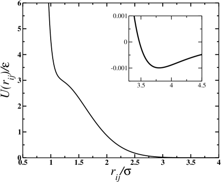
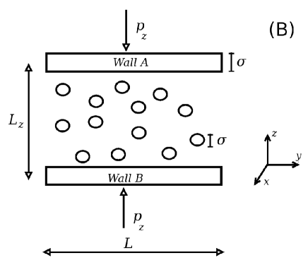
Figure 1: (A) Interaction potential as function of the particles separation. (B) Schematic depiction of the simulation cell with the fluid and walls. The walls are separated by a distance $L_{z}$, have thickness $\sigma$ and an external pressure $p_{z}$ is applied in the $z$ direction.

The anomalous fluid was modeled as spherical core-softened particles with mass $m$ and effective diameter $\sigma$. The interaction is obtained by the potential Oliveira06a

$$\frac{U(r_{ij})}{\varepsilon}=4\left[\left(\frac{\sigma}{r_{ij}}\right)^{12}-\left(\frac{\sigma}{r_{ij}}\right)^{6}\right]+u_{0}{\rm{exp}}\left[-\frac{1}{c_{0}^{2}}\left(\frac{r_{ij}-r_{0}}{\sigma}\right)^{2}\right]$$ (1)

where $r_{ij}=|\vec{r}_{i}-\vec{r}_{j}|$ is the distance between the two fluid particles $i$ and $j$. This equation has two terms: the first one is the standard 12-6 Lennard-Jones (LJ) potential AllenTild and the second one is a gaussian centered at $r_{0}$, with depth $u_{0}$ and width $c_{0}$. Using the parameters $u_{0}=5.0$, $c=1.0$ and $r_{0}/\sigma=0.7$ this equation represents a two length scale potential, with one scale at $r_{ij}\equiv r_{1}\approx 1.2\sigma$, where the force has a local minimum, and the other scale at $r_{ij}\equiv r_{2}\approx 2\sigma$, where the fraction of imaginary modes has a local minimum Oliveira10 . The potential is shown in Fig. 1(A). Despite the mathematical simplicity this model exhibits the bulk water-like anomalies Oliveira06a ; Oliveira06b ; Kell67 ; Angell76 as well confined water properties Bordin12b ; Bordin13a ; Krott13a ; Krott13b ; Krott14a ; Bordin14a ; Bordin14b .

Was already shown that the confined fluid properties are strongly affected by the nanopore mobility Krott13b ; Bordin14a ; Bernardi10 ; Yong13 . Since we want to fix the pressure at high values, we explore behavior of this anomalous fluid confined in a non-rigid nanopore Krott13b ; Bordin14a ; Bernardi10 ; Yong13 . The nanopore was modeled as two parallel flat plates. The simulation box is a parallelepiped with dimensions $L_{x}\times L_{y}\times L_{z}$. The model for the fluid-wall system is illustrated in Fig. 1(B). Two walls, A in the top and B in the bottom, are placed in the limits of the $z$-direction of the simulation box. The sizes $L_{x}$ and $L_{y}$ are fixed in all simulations, and defined as $L_{x}=L_{y}=L=40\sigma$. The values of $L_{z}$ depends on the applied pressure $p_{z}$ in the $z$-direction. The system was modeled in the $NLp_{z}T$ ensemble using the Lupkowski and van Smol method of fluctuating confining walls LupSmol90 to fix $p_{z}$.

The walls are flat and purely repulsive, and the interaction between a fluid particle and these walls is represented by the Weeks-Chandler-Andersen (WCA) WCA71 potential,

$$U^{\rm{WCA}}(z_{ij})=\left\{\begin{array}[]{ll}U_{{\rm{LJ}}}(z_{ij})-U_{{\rm{LJ}}}(z_{c})\;,\qquad z_{ij}\leq r_{c}\;,\\ 0\;,\qquad\qquad\qquad\qquad\quad z_{ij}>r_{c}\;.\end{array}\right.$$ (2)

Here, $U_{{\rm{LJ}}}$ is the standard 12-6 LJ potential, included in the first term of Eq. (1), and $r_{c}=2^{1/6}\sigma$ is the usual cutoff for the WCA potential. Also, the term $z_{ij}$ measures the distance between the wall at $j$ position and the $z$-coordinate of the fluid particle $i$.

II.2 The simulation details

The physical quantities are computed in the standard LJ units AllenTild ,

$$r^{*}\equiv\frac{r}{\sigma}\;,\quad\rho^{*}\equiv\rho\sigma^{3}\;,\quad\mbox{and}\quad t^{*}\equiv t\left(\frac{\epsilon}{m\sigma^{2}}\right)^{1/2}\;,$$ (3)

for distance, density of particles and time , respectively, and

$$p^{*}\equiv\frac{p\sigma^{3}}{\epsilon}\quad\mbox{and}\quad T^{*}\equiv\frac{k_{B}T}{\epsilon}$$ (4)

for the pressure and temperature, respectively. Since all physical quantities are defined in reduced LJ units in this paper, the ^∗ is omitted, in order to simplify the discussion.

The simulations were performed at constant number of particles, constant $L$, constant perpendicular pressure and constant temperature ($NLp_{z}T$ ensemble). The perpendicular pressure was fixed using the Lupkowski and van Smol method LupSmol90 . In this technique, the nanopore walls had translational freedom in the $z$-direction, acting like a piston in the fluid, and a constant force controls the pressure applied in the confined direction. This scenario is similar to some recent experiments on water confined inside nanopores at externally applied high pressures Alabarse14 ; Catafesta14 . Considering the nanopore flexible walls, the resulting force in a fluid particle is then

$$\vec{F}_{R}=-\vec{\nabla}U+\vec{F}_{iwA}(\vec{r}_{iA})+\vec{F}_{iwB}(\vec{r}_{iB})\;,$$ (5)

where $\vec{F}_{iwA(B)}$ indicates the interaction between the particle $i$ and the wall $A(B)$. Since the walls are non-rigid and time-dependent, we have to solve the equations of motion for $A$ and $B$,

$$m_{w}\vec{a}_{A(B)}=p_{z}S_{w}\vec{n}_{A(B)}-\sum_{i=1}^{N}\vec{F}_{iwA(B)}(\vec{r}_{iA(B)}),$$ (6)

where $m_{w}$ is the piston mass, $p_{z}$ is the applied pressure in the system, $S_{w}$ is the wall area and $\vec{n}_{A}$ is an unitary vector in positive $z$-direction, while $\vec{n}_{B}$ is a negative unitary vector. Both pistons ($A$ and $B$) have mass $m_{w}=m$, width $\sigma$ and area equal to $S_{w}=L^{2}$.

The system temperature was fixed using the Nose-Hoover heat-bath with a coupling parameter $Q=2$ and was varied from small temperatures, $T=0.01$ to higher temperatures $T=0.4$. Standard periodic boundary conditions were applied in the $x$ and $y$ directions. The equations of motion for the fluid particles and the walls were integrated using the velocity Verlet algorithm, with a time step $\delta t=0.001$.

Five independent runs were performed to evaluate the properties of the confined fluid. The initial system was generated placing the fluid particles randomly in the space between the walls. The initial displacement for the simulations was $L_{z0}=15$. We performed $5\times 10^{5}$ steps to equilibrate the system. This equilibration time was taken in order to ensure that the walls reached the equilibrium position for the fixed values of $p_{z}$. These steps are then followed by $1\times 10^{8}$ steps for the results production stage. The large production time is necessary to observe the correct dynamical behavior of the confined fluid.

The fluid-fluid interaction, Eq. (1), has a cutoff radius $r_{\rm cut}/\sigma=3.5$. The number of particles was fixed in $N=1000$, and four values of pressure where simulated: $p_{z}=7.0$, 8.0, 9.0 and 10.0. Due to the excluded volume originated by the nanopore-fluid interaction, the distance $L_{z}$ between the walls needs to be corrected to an effective distance Ku05 ; kumar07 , $L_{ze}$, that can be approach by $L_{ze}\approx L_{z}-1$. The effective distance, due the nanopore flexibility, will oscillate around an average value $\langle L_{ze}\rangle$ and the average density will be $\rho=N/(\langle L_{ze}\rangle L^{2})$. Also, it is important to reinforce that, since $N$ is fixed for all simulations, the distinct values for density are obtained by the variation in pressure and temperature, and consequently variation in plates separation, $L_{z}$.

To analyze the fluid dynamical properties we computed the lateral mean square displacement (MSD) using Einstein relation

$$\langle[\vec{r}_{||}(t)-\vec{r}_{||}(t_{0})]^{2}\rangle=\langle\Delta\vec{r}_{||}(t)^{2}\rangle=4Dt^{\alpha}\;,$$ (7)

where $\vec{r}_{||}(t_{0})=(x(t_{0})^{2}+y(t_{0})^{2})^{1/2}$ and $\vec{r}_{||}(t)=(x(t)^{2}+y(t)^{2})^{1/2}$ denote the parallel coordinate of the confined anomalous fluid particle at a time $t_{0}$ and at a later time $t$, respectively. We should address that the mean square displacement was calculated considering all the particles in the system. Nanoconfined fluids assumes a layered structure. Despite this, the evaluation of $\langle[\vec{r}_{||}(t)-\vec{r}_{||}(t_{0})]^{2}\rangle$ for each layer can lead to a spurious statistics for the result, since the number of particles in each layer is small and the particles can move from one layer to another, leading to a poor time average in Eq. 7. Depending on the scaling law between $\Delta\vec{r}_{||}(t)^{2}$ and $t$ in the limit $t\rightarrow\infty$, different diffusion mechanisms can be identified: $\alpha<1.0$ refers to a subdiffusive regime, with $\alpha=0.5$ identifying a single file regime Farimani11 . $\alpha=1.0$ stands for a Fickian diffusion whereas $\alpha>1.0$ defines the superdiffusive regime, and $\alpha=2.0$ refers to a ballistic diffusion Striolo06 ; Zheng12 .

In order to define the fluid characteristics at different distances from the nanopore walls, the structure of the fluid layers was analyzed using the radial distribution function $g(r_{||})$, defined as

$$g(r_{||})\equiv\frac{1}{\rho^{2}V}\sum_{i\neq j}\delta(r-r_{ij})\left[\theta\left(\left|z_{i}-z_{j}\right|\right)-\theta\left(\left|z_{i}-z_{j}\right|-\delta z\right)\right].$$ (8)

where the Heaviside function $\theta(x)$ restricts the sum of particle pair in a slab of thickness $\delta z=1.0$ close to the wall or $\delta z=1.0$ away from the walls.

In all simulations the mean variation in the system size induced by the wall fluctuations are smaller than $2\%$. Data errors are smaller than the data points and are not shown. The data obtained in the equilibration period was not considered for the quantities evaluation.

III Results and Discussion

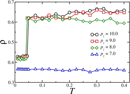
Figure 2: $\rho\times T$ phase diagram for the confined anomalous fluid for different isobaric curves: $p_{z}=7.0$, 8.0, 9.0 and 10.0. Errors bars are smaller than the data point.

The thermodynamical behavior of the confined anomalous fluid is shown in Fig. 2. The isobaric curves at lateral pressure $p_{z}=7.0$, 8.0, 9.0 and 10.0 show distinct behavior. For the smaller pressure, $p_{z}=7.0$, the density as function of the system temperature does not vary significatively with the temperature. This result agrees with our previous findings Bordin14a that indicates that for flexible walls and pressures $p_{z}<6.0$ the density varies smoothly with the temperature. However, for higher values of $p_{z}$ transition from low density to high density is observed as the temperature is varied. For the pressures values $p_{z}=$ 8.0 and 9.0 the fluid density exhibits a jump from the dimensionless density $\rho\approx 0.45$ to the density $\rho\approx 0.6$ at $T=0.45$. For $p_{z}=10.0$ the change in the density occurs at the temperature $T=0.5$.

This transition is related to a change in the system’s conformation. Nanoconfined fluids assume a layered structure Nanok09 . The number of layers depend in the different nanopores geometries, on the nanotube radius and on the plates separation  Bordin12b ; Bordin13a ; Krott13b ; Bordin14a ; Bordin14b . Since the number of particles in our system is fixed, the density change observed in the Figure 2 implies change in the distance between the two plates and consequently in the number of layers.

Fig. 3(A) illustrates the density distribution versus the distance between the plates for $p_{z}=10.0$ at different temperatures. For low temperatures, the system forms three layers: two contact layers and a central layer. For higher temperatures the central layer melts and the fluid is structured in two contact layers. The behavior for $p_{z}=8.0$ and 9.0 are similar to the case $p_{z}=10.0$ and, for simplicity, these results are not shown.

For $p_{z}=7.0$, the fluid has three layers for all the temperatures studied as shown in Fig. 3(B).

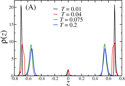
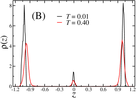
Figure 3: Confined fluid density profile $\rho(z)$ for $p_{z}=10.0$ and $T=0.01$, 0.04, 0.075 and 0.2 (A) and $p_{z}=7.0$ and $T=0.01$ and 0.4 (B).

The transition from low to high density as the temperature is increased at constant pressure is quite counterintuitive. Usually the increase of density is associated with decrease of entropy. Here, however, it is the contrary. This anomalous behavior follows from the same mechanism of the increase of density at constant pressure, the bulk density anomaly.

At low temperatures particles in the same layer minimize the energy Eq. (1) by being at a distance distance $r_{2}\approx 2$, the second length in the potential, as shown in Fig. 4. Because the pressure is high, the distance between the planes is smaller than any of the two length scales.

At these low temperatures both the contact planes are quite structured as shown in Fig. 4(A) while the central plane is solid-like as illustrated in Fig. 4(B). These structures, similarly to the low temperature liquid water, have low density but high order and consequently low entropy. As the temperature is increased, the central layer melts. The two contact layers approach, being at the first length scale, namely $r_{1}\approx 1.2$ distance from each other as shown in Fig. 3. Inside each layer particles are at $r_{2}\approx 2$ distant from each other. As the temperature is increased, the order inside each layer decreases as shown in Fig. 4(A) and the entropy increases. Therefore, the denser system is more entropic similarly with what happens with water at the region of the density anomaly.

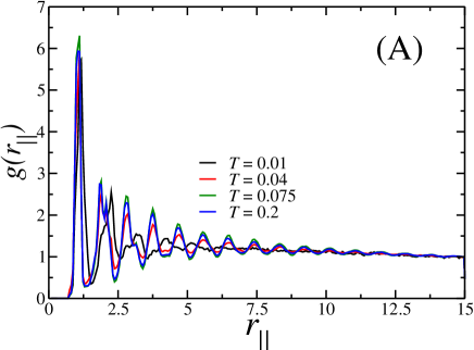
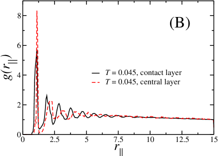
Figure 4: (A) Radial distribution function $g(r_{||})$ for the contact layer for the confined fluid at $p_{z}=10.0$ and $T=0.01$, 0.04, 0.075 and 0.2. (B) $g(r_{||})$ for the contact and central layer at $p_{z}=10.0$ and $T=0.045$.

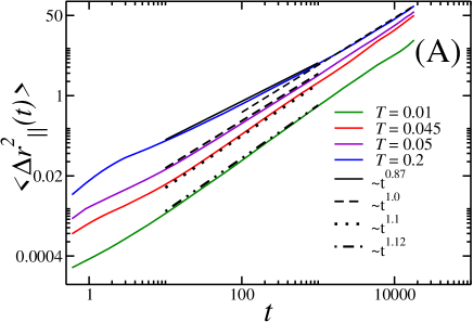
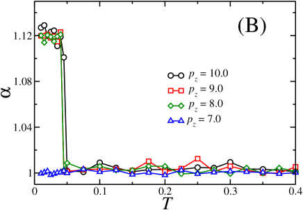
Figure 5: (A) Lateral mean square displacement $\langle\Delta r^{2}_{||}(t)\rangle$ as function of simulation time for external pressure $p_{z}=10.0$ and $T=0.01$, 0.045, 0.05 and 0.2. Reference curves slopes are also shown. (B) Temperature dependence of $\alpha$ for $p_{z}=8.0$, 9.0 and 10.0.

What is the relation between this layer transition and the mobility of the nanoconfined particles? The layers structure can provide both a restriction or an enhancement of the mobility of the particles Bordin12b ; Krott13b ; Bordin14b . In order to illustrate this point we study the mean square displacement (MSD) as a function of time for different temperatures and pressures. Fig. 7(A) shows the MSD versus time for $p_{z}=10.0$ and $T=0.01,0.045,0.05,0.2$. In order to understand the behavior of the mobility in the framework of Einstein Equation, Eq. (7), the exponent $\alpha$ is computed in all the studied cases. Fickian diffusion if observed for $p_{z}=8.0$, 9.0 and 10.0 for temperatures above the three-to-two layers transition. This behavior was obtained after long time simulation. For shorter simulation times the system exhibits an apparent subdiffusive regime, where $\alpha<1.0$. This behavior was also obtained for water confined in nanotubes Zheng12 . In our case, as in the nanotube systems Zheng12 , as $t\rightarrow\infty$ (see Fig. 5(A)) the Fickian diffusion is recovered. As example, we show in the purple curve of Fig. 5(A) the behavior for $T=0.05$ and $p_{z}=10.0$.

For low temperatures, below the three-to-two layer transition, however, the systems for $p_{z}=8.0,9.0$ and $10.0$ exhibit a superdiffusive behavior with $\alpha>1$.

Fig. 5(B) shows the behavior of $\alpha$ versus temperature illustrating that the transition temperature from non-fickian to fickian regime coincides with the transition from three-to-two layers with the increase of density shown on Fig. 2.

The transition between layers followed by change in the exponent $\alpha$ was also observed in atomistic models for water Zheng12 ; Farimani11 . In these cases, it is not clear is the anomalous diffusion are in equilibrium of if they are na artifact of the short simulation times In our case, the coarse grained potential provide us with an easy way to perform long simulations and we can ensure that the system is equilibrated.

IV Conclusion

We have studied the behavior of a anomalous fluid confined inside a flexible nanopore at high external pressure. Our results show a structural phase transition in the $\rho\times T$ phase diagram for isobaric curves with $p_{z}\geq 8.0$. This phase transition corresponds to a three to two layers transition, and it is associated to a transition between a superdiffusive regime and a Fickian diffusion. These results indicates that anomalous fluids, as water, can exhibit a superdiffusion regime at small temperature and high pressures associated with the same mechanism that at the bulk generate the density anomaly

V Acknowledgments

We thanks the Brazilian agencies CNPq, INCT-FCx, and Capes for the financial support. We also thanks to TSSC - Grupo de Teoria e Simulação em Sistemas Complexos at UFPel for the computer clusters.

References

- (1) P. Tabeling and L. Bocquet, Lab on a Chip 14, 3143 (2014).
- (2) M. Majunder, N. Chopra, R. Andrews, and B. J. Hinds, Nature 438, 44 (2005).
- (3) J. K. Holt et al., Science 312, 1034 (2006).
- (4) M. Whitby, L. Cagnon, and M. T. ans N. Quirke, Nanoletters 8, 2632 (2008).
- (5) X. Qin, Q. Yuan, Y. Zhao, S. Xie, and Z. Liu, Nanoletters 11, 2173 (2011).
- (6) K. P. Lee, H. Leese, and D. Mattia, Nanoscale 4, 2621 (2012).
- (7) T. Nanok, N. Artrith, P. Pantu, P. A. Bopp, and J. Limtrakul, J. Phys. Chem. A 113, 2103 (2009).
- (8) S. T. Cui, P. T. Cummings, and H. D. Cochran, J. Chem. Phys. 114, 7189 (2001).
- (9) A. Jabbarzadeh, P. Harrowell, and R. I. Tanner, J. Chem. Phys. 125, 034703 (2006).
- (10) F. G. Alabarse et al., Phys. Rev. Lett. 109, 035701 (2012).
- (11) A. B. Farimani and N. R. Aluru, J. Phys. Chem. B 115, 12145 (2011).
- (12) A. Striolo, Nanoletters 4, 633 (2006).
- (13) S. Jakobtorweihen, M. G. Verbeek, C. P. Lowe, . F. J. Keil, and B. Smit, Phys. Rev. Lett. 95, 044501 (2005).
- (14) H. Chen, J. K. Johnson, and D. S. Sholl, J. Phys. Chem. B Lett. 110, 1971 (2006).
- (15) M. Chaplin, Sixty-nine anomalies of water, http://www.lsbu.ac.uk/water/anmlies.html, 2013.
- (16) G. S. Kell, J. Chem. Eng. Data 20, 97 (1975).
- (17) C. A. Angell, E. D. Finch, and P. Bach, J. Chem. Phys. 65, 3065 (1976).
- (18) F. X. Prielmeier, E. W. Lang, R. J. Speedy, and H.-D. Lüdemann, Phys. Rev. Lett. 59, 1128 (1987).
- (19) H. Thurn and J. Ruska, J. Non-Cryst. Solids 22, 331 (1976).
- (20) Handbook of Chemistry and Physics, CRC Press, Boca Raton, Florida, 65 ed. edition edition, 1984.
- (21) G. E. Sauer and L. B. Borst, Science 158, 1567 (1967).
- (22) S. J. Kennedy and J. C. Wheeler, J. Chem. Phys. 78, 1523 (1983).
- (23) T. Tsuchiya, J. Phys. Soc. Jpn. 60, 227 (1991).
- (24) P. T. Cummings and G. Stell, Mol. Phys. 43, 1267 (1981).
- (25) M. Togaya, Phys. Rev. Lett. 79, 2474 (1997).
- (26) C. A. Angell, R. D. Bressel, M. Hemmatti, E. J. Sare, and J. C. Tucker, Phys. Chem. Chem. Phys. 2, 1559 (2000).
- (27) M. S. Shell, P. G. Debenedetti, and A. Z. Panagiotopoulos, Phys. Rev. E 66, 011202 (2002).
- (28) R. Sharma, S. N. Chakraborty, and C. Chakravarty, J. Chem. Phys. 125, 204501 (2006).
- (29) S. Sastry and C. A. Angell, Nature Mater. 2, 739 (2003).
- (30) P. A. Netz, F. W. Starr, H. E. Stanley, and M. C. Barbosa, J. Chem. Phys. 115, 344 (2001).
- (31) P. A. Netz, F. W. Starr, M. C. Barbosa, and H. E. Stanley, Physica A 314, 470 (2002).
- (32) S.-H. Chen et al., Proc. Natl. Acad. Sci. USA 103, 12974 (2006).
- (33) T. Morishita, Phys. Rev. E 72, 021201 (2005).
- (34) P. Vilaseca and G. Franzese, Journal of Non-Crystalline Solids 357, 419 (2011).
- (35) Y. Zheng, H. Ye, Z. Zhang, and H. Zhang, Phys. Chem. Chem. Phys. 14, 964 (2012).
- (36) J. R. Bordin, L. Krott, and M. C. Barbosa, J. Phys. Chem. C 118, 9497 (2014).
- (37) L. Krott and J. R. Bordin, J. Chem. Phys. 139, 154502 (2013).
- (38) A. B. de Oliveira, P. A. Netz, T. Colla, and M. C. Barbosa, J. Chem. Phys. 124, 084505 (2006).
- (39) A. B. de Oliveira, P. A. Netz, T. Colla, and M. C. Barbosa, J. Chem. Phys. 125, 124503 (2006).
- (40) L. Krott and M. C. Barbosa, J. Chem. Phys. 138, 084505 (2013).
- (41) L. Krott and M. C. Barbosa, Phys. Rev. E 89, 012110 (2014).
- (42) J. R. Bordin, A. B. de Oliveira, A. Diehl, and M. C. Barbosa, J. Chem. Phys 137, 084504 (2012).
- (43) J. R. Bordin, A. Diehl, and M. C. Barbosa, J. Phys. Chem. B 117, 7047 (2013).
- (44) J. R. Bordin, J. S. Soares, A. Diehl, and M. C. Barbosa, J. Chem Phys. 140, 194504 (2014).
- (45) P. Allen and D. J. Tildesley, Computer Simulation of Liquids, Oxford University Press, Oxford, 1987.
- (46) A. B. de Oliveira, E. Salcedo, C. Chakravarty, and M. C. Barbosa, J. Chem. Phys. 132, 234509 (2010).
- (47) G. S. Kell, J. Chem. Eng. Data 12, 66 (1967).
- (48) C. A. Angell, E. D. Finch, and P. Bach, J. Chem. Phys. 65, 3063 (1976).
- (49) S. Berbardi, B. D. Todd, and D. J. Searles, J. Chem. Phys. 132, 244706 (2010).
- (50) X. Yong and L. T. Zhang, J. Chem. Phys. 138, 084503 (2013).
- (51) M. Lupowski and F. van Smol, J. Chem. Phys. 93, 737 (1990).
- (52) J. D. Weeks, D. Chandler, and H. C. Andersen, J. Chem. Phys. 54, 5237 (1971).
- (53) F. G. Alabarse et al., J. Phys. Chem. C 118, 3651 (2014).
- (54) J. Catrafesta et al., Phys. Chem. Chem. Phys. 16, 12202 (2014).
- (55) P. Kumar, S. V. Buldyrev, F. Sciortino, E. Zaccarelli, and H. E. Stanley, Phys. Rev. E 72, 021501 (2005).
- (56) P. Kumar, F. W. Starr, S. V. Buldyrev, and H. E. Stanley, Phys. Rev. E 72, 011202 (2007).
- (57) A. Striolo, Nanoletters 6, 633 (2006).