Fractal Butterflies of Dirac Fermions in Monolayer and Bilayer graphene

Abstract

We present an overview of the theoretical understanding of Hofstadter butterflies in monolayer and bilayer graphene. After a brief introduction on the past work in conventional semiconductor systems, we discuss the novel electronic properties of monolayer and bilayer graphene that helped to detect experimentally the fractal nature of the energy spectrum. We have discussed the theoretical background on the Moiré pattern in graphene. This pattern was crucial in determining the butterfly structure. We have also touched upon the role of electron-electron interaction in the butterfly pattern in graphene. We conclude by discussing the future prospects of butterfly search, especially for interacting Dirac fermions.

I Introduction

The dynamics of an electron in a periodic potential subjected to a perpendicular magnetic field has remained an interesting problem for more than half a century review_2000 ; harper ; langbein ; hofstadter . Within the nearest neighbor tight-binding description of the periodic potential the energy spectrum of an electron is described by the Harper equation harper . Numerical solution of this equation hofstadter shows that the applied magnetic field splits the Bloch bands into subbands and gaps. The resulting energy spectrum, when plotted as a function of the magnetic flux per lattice cell, reveals a fractal pattern (a self-similar pattern that repeats at every scale) mandelbrot that is known in the literature as Hofstadter’s butterfly (due to the pattern resembling the butterflies). This is the first example of the fractal pattern realized in the energy spectra of a physical system.

A few experimental efforts to detect the butterflies have been reported in the literature. The earlier ones involved artificial lateral superlattices on semiconductor nanostructures geisler_04_1 ; geisler_04_2 ; albrecht_01 ; albrecht_02 ; ensslin_96_1 ; ensslin_96_2 , more precisely the antidot lattice structures with periods of $\sim$100 nm. The large period (as opposed to those in natural crystals) of the artificial superlattices helps to keep the magnetic field in a reasonable range of values to observe the fractal pattern. Measurements of quantized Hall conductance in such a structure indicated, albeit indirectly, the complex pattern of gaps that were expected in the butterfly spectrum. Hofstadter butterfly patterns were also predicted to occur in other totally unrelated systems, such as, propagation of microwaves through a waveguide with a periodic array of scatterers microwave or more recently, with ultracold atoms in optical lattices optical_lattice_1 ; optical_lattice_2 .

Graphene, the single layer of carbon atoms, arranged in a hexagonal lattice and contains an wealth of unusual electronic properties graphene_book ; abergeletal ; chapter ; xu_review has turned out to be the ideal system in the quest of fractal butterflies. The Dirac fermions in monolayer and bilayer graphene chapter are the most promising objects thus far, where the signature of the recursive pattern of the Hofstadter butterfly has been unambiguously reported dean_13 ; hunt_13 ; geim_13 . Here the periodic lattice with a period of $\sim$ 10 nm was created by the Moiré pattern that appears when graphene is placed on a plane of hexagonal boron nitride (h-BN) with a twist hbn ; moire_1 ; moire_2 . Being ultraflat and free of charged impurities, h-BN has been the best substrate for graphene having high-mobility charged fermions hbn . Some theoretical studies have been reported earlier in the literature on the butterfly pattern in monolayer rhim and bilayer graphene nemec .

The paper is organized as follows. In Sect. II, we briefly describe the background materials leading to the Hofstadter butterfly. The situation in conventional semiconductor systems is presented in Sect. III. Sect. IV deals with the theories of the butterfly pattern in monolayer graphene, while the theoretical intricacies in bilayer graphene are presented in Sect. V. The case of the many-electron system, in particular the influence of the electron-electron interaction on the Hofstadter butterfly pattern is described in Sect. VI. The concluding remarks are to be found in Sect. VII.

II Electrons in a periodic potential and an external magnetic field: Hofstadter butterfly

The dynamics of a two-dimensional (2D) electron in a periodic potential is described by the Hamiltonian

$${\cal H}={\cal H}_{0}(p_{x},p_{y})+V(x,y),$$ (1)

which consists of the kinetic energy term ${\cal H}_{0}(p_{x},p_{y})$ and the periodic potential $V(x,y)$. The most important characteristics of this periodic potential, which determines the dynamics of an electron in a magnetic field is the area $S_{0}$ of the unit cell of the periodic structure of $V(x,y)$. For a structure of a simple square lattice type, which is characterized by the lattice constant $a_{0}$, the area of a unit cell is $S_{0}=a_{0}^{2}$. The magnetic field $B$ is introduced in the Hamiltonian (1) via the Peierls substitution, which replaces the momentum $(p_{x},p_{y})$ by the generalized expression $(p_{x}-eA_{x}/c,p_{y}-eA_{y}/c)$. Here $(A_{x},A_{y})$ is the vector potential. We choose the vector potential in the Landau gauge $\vec{A}=(0,Bx)$. The corresponding Hamiltonian then becomes

$${\cal H}={\cal H}_{0}(p_{x}-exB)+V(x,y).$$ (2)

The energy spectra of the Hamiltonian (2) as a function of the magnetic field has the unique fractal structure. Such a structure has a more clear description in the two limiting cases of weak and strong magnetic field. In the case of the weak magnetic field, first, the periodic potential results in the formation of the Bloch bands and then the external magnetic field splits each Bloch band of the periodic potential into minibands of the Landau level (LL) type. In a weak magnetic field, the coupling of different bands can be disregarded. The corresponding Schrödinger equation, which determines the energy spectrum of the system, has a simple form in the tight-binding approximation for the periodic potential, for which the energy dispersion within a single band is

$$E(p_{x},p_{y})=2\Delta_{0}\left(\cos(p_{x}a_{0}/\hbar)+\cos(p_{y}a_{0}/\hbar)\right),$$ (3)

where a simple square lattice structure with lattice constant $a_{0}$ was assumed. In an external magnetic field, the wave function which is defined at the lattice points $(ma_{0},na_{0})$, has the form $\Psi(ma,na)=e^{ik_{y}n}\psi_{m}$. The corresponding Schrödinger equation reduces to a one-dimensional equation – the so called Harper equation harper

$$\psi_{m+1}+\psi_{m-1}+2\cos\left(2\pi m\tilde{\alpha}-k_{y}\right)\psi_{m}=\varepsilon\psi_{m},$$ (4)

where $\varepsilon=E/\Delta_{0}$ and $\tilde{\alpha}=\Phi/\Phi_{0}$. Here $\Phi=BS_{0}=Ba_{0}^{2}$ is the magnetic flux through a unit cell and $\Phi_{0}=hc/e$ is the magnetic flux quantum. Therefore, the dimensionless parameter $\tilde{\alpha}$ is the magnetic flux through a unit cell measured in units of the flux quantum. The energy spectra, determined by the Harper equation (4), is a periodic function of the parameter $\tilde{\alpha}$ with period 1. Hence it is enough to consider only the values of $\tilde{\alpha}$ within the range $0<\tilde{\alpha}<1$. The remarkable property of the Harper equation (4) is that although the corresponding Hamiltonian is an analytical function of $\tilde{\alpha}$, the energy spectrum [Eq. (4)] is very sensitive to the value of $\tilde{\alpha}$. At rational values of $\tilde{\alpha}=p/q$ the energy spectrum has $q$ bands separated by $q-1$ gaps, where each band is $p$ fold degenerate. As a function of $\tilde{\alpha}$ the energy spectrum [Eq. (4)] has a fractal structure that is known as the Hofstadter butterfly hofstadter . This structure is shown in Fig. 1. The thermodynamic potential $\Omega_{b}(T,\mu,\tilde{\alpha})$, corresponding of the system described by the Harper equation (4), satisfies the following symmetry property avron

$$\Omega_{b}(T,\mu,\tilde{\alpha})=\Omega_{b}(T,\mu,-\tilde{\alpha})=\Omega_{b}(T,\mu,\tilde{\alpha}+1),$$ (5)

which means that the thermodynamic properties of the system are determined by $0<\tilde{\alpha}<1/2$ and $\mu<0$. Here $\mu$ is the chemical potential.

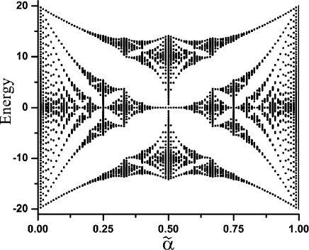
Figure 1: Energy spectra (Hofstadter butterfly) of the Harper equation (4). Parameter $\tilde{\alpha}$ is the magnetic flux per unit cell in units of flux quantum.

In a strong magnetic field the energy spectra of the system also show the Hofstadter butterfly fractal structure. Now the periodic potential should be considered as a weak perturbation, which results in a splitting of the corresponding LLs, formed by the strong magnetic field. For a weak periodic potential the inter LL coupling can be disregarded. Then the splitting of a given LL is described by the same Harper-type equation,

$$\psi_{m+1}+\psi_{m-1}+2\cos\left(2\pi m\alpha-k_{y}\right)\psi_{m}=\varepsilon\psi_{m},$$ (6)

but now the parameter, which determine the fractal structure of the energy spectrum, is $\alpha=1/\tilde{\alpha}=\Phi_{0}/\Phi$ - inverse magnetic flux though a unit cell in units of the flux quantum. Therefore, for $0<\alpha<1$ the energy spectrum has a structure similar to the one shown in Fig. 1. The Hofstadter butterfly energy spectra is realized either as a splitting of the Bloch band by a weak magnetic field or as a splitting of a LL by the weak periodic potential. The thermodynamics properties of these two systems are related by the duality transformation avron

$$\Omega_{L}(T,\mu,\alpha)=\alpha\Omega_{b}(T,\mu,\tilde{\alpha}),$$ (7)

where $\Omega_{L}(T,\mu,\alpha)$ is the thermodynamic potential within a single LL and weak periodic potential.

For intermediate values of the magnetic field, the mixing of the LL by the periodic potential or the mixing of Bloch bands by the magnetic field becomes strong. This will modify the universality of the butterfly structure and add some system-dependent features. In the following sections we consider the limits of high and intermediate magnetic fields for conventional semiconductor systems and the monolayer and bilayer graphene.

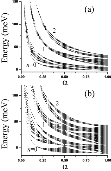
Figure 2: Single-electron energy spectra of conventional semiconductor systems with parabolic dispersion relation. The period of the potential is $a_{0}=20$ nm and its amplitude is (a) $V_{0}=10$ meV and (b) $V_{0}=20$ meV. The energy spectra are shown as a function of the parameter $\alpha=\Phi_{0}/\Phi$. The numbers indicate the LL index $n$.

III Conventional semiconductor systems: strong field limit

For strong and intermediate magnetic fields, the periodic potential is considered as a perturbation, which can modify and mix the states of the zero-order Hamiltonian, consisting of the kinetic part only ${\cal H}_{0}(p_{x}-eA_{x}/c,p_{y}-eA_{y}/c)$. For conventional semiconductor systems the zero-order Hamiltonian is described by the parabolic dispersion relation, $p^{2}/2m$. The transverse magnetic field results in Landau quantization where the LLs are characterized by the Landau level index $n=0,1,2,\ldots$ with energies $E_{n}=(n+1/2)\hbar\omega_{c,B}$. Here $\omega_{c,B}=eB/mc$ is the cyclotron frequency. The corresponding Landau wave functions $\phi_{n,k}$ have the form

$$\phi_{n,k}(x,y)=\frac{e^{iky}}{\sqrt{L}}\frac{e^{-(x-x_{k})^{2}/2\ell_{0}^{2}}}{\sqrt{\pi^{1/2}\ell_{0}2^{n}n!}}H_{n}(x-x_{k}),$$ (8)

where $L$ is the length of a sample in the $y$ direction, $k$ is the $y$ component of the electron wave vector, $\ell_{0}=\sqrt{c\hbar/eB}$ is the magnetic length, $x_{k}=k\ell^{2}_{0}$, and $H_{n}(x)$ are the Hermite polynomials.

We consider a system in a periodic external potential that has the form

$$V(x,y)=V_{0}\left[\cos(q_{x}x)+\cos(q_{y}y)\right],$$ (9)

where $V_{0}$ is the amplitude of the periodic potential, $q_{x}=q_{y}=q_{0}=2\pi/a_{0}$, and $a_{0}$ is a period of the external potential $V(x,y)$. The periodic potential mixes the electron states $\phi_{n,k}$ within a single LL, i.e., states with the same value of LL index $n$ and different values of $k$, and also mixtures the states of different LLs with different indices $n$. The strength of the mixing is determined by the matrix elements of the periodic potential $V(x,y)$ between the LL states $\phi_{n,k}$.

The matrix elements of the periodic potential $V(x,y)$ in the basis $\phi_{n,k}(x,y)$ are

$$\left\langle\phi_{n^{\prime},k^{\prime}}\right|\cos(q_{0}y)\left|\phi_{n,k}\right\rangle=$$

$$\frac{i^{n-n^{\prime}}}{2}\left\{\delta_{k^{\prime},k+q_{0}}+(-1)^{n-n^{\prime}}\delta_{k^{\prime},k-q_{0}}\right\}M_{n^{\prime},n}$$ (10)

and

$$\left\langle\phi_{n^{\prime},k^{\prime}}\right|\cos(q_{0}x)\left|\phi_{n,k}\right\rangle=\frac{\delta_{k^{\prime},k}}{2}e^{-iq_{0}k\ell_{0}^{2}}\left[1+(-1)^{n-n^{\prime}}\right]M_{n^{\prime},n}.$$ (11)

Here

$$M_{n^{\prime},n}=\left(\frac{m!}{M!}\right)^{1/2}e^{-Q/2}Q^{|n^{\prime}-n|/2}L_{m}^{|n^{\prime}-n|}(Q),$$ (12)

$Q=q_{0}^{2}\ell_{0}^{2}/2$, $m=\min(n^{\prime},n)$, $M=\max(n^{\prime},n)$.

The matrix elements (10) and (11) determine the mixture of the LL states introduced by the periodic potential. While the component of the potential periodic in the $x$ direction [Eq. (11)] couples only the states with the same value of the wave vector $k$, the component periodic in the $y$ direction couples the states with the wave vectors separated by $q_{0}$. Within a single LL the potential periodic in the $x$ direction modifies the energy of each Landau state. As a result the energy of the Landau state within a given LL becomes a periodic function of $q_{0}kl_{0}^{2}$. Additional coupling of the states separated by $q_{0}$, which is determined by Eq. (10), results in the formation of the band structure when $q_{0}^{2}l_{0}^{2}$ becomes a rational fraction of $2\pi$, which is exactly the condition that the parameter $\alpha$ is rational. It follows from Eqs. (10)-(11) that for a given LL with index $n$ the effective amplitude of the periodic potential acquires an additional factor and becomes $\propto V_{0}M_{n,n}\propto L_{n}(q_{0}^{2}\ell_{0}^{2}/2)=L_{n}(\pi\alpha)$. These renormalized amplitudes determine the width of the corresponding bands. At values of $\alpha$ where $L_{n}(\pi\alpha)=0$, all bands have zero width which correspond to the flatband condition geisler_04_1 ; geisler_04_2 .

In general, the expressions for the matrix elements (11) and (10) can be used to find the energy spectra of any finite number of LLs, taking into account the coupling of different LLs introduced by the periodic potential. For a given value of $k$ within the interval $0<k<q_{0}$, a finite set of basis wave functions $\phi_{n,k}$, $\phi_{n,k+q_{0}}$, $\phi_{n,k+2q_{0}}$,…, $\phi_{n,k+N_{x}q_{0}}$ is considered. Here $n=0,\ldots,N_{L}$, $N_{L}$ is the number of LLs, and $N_{x}$ determines the size of the system in the $x$ direction: $L_{x}=N_{x}q_{0}\ell_{0}^{2}$. The matrix elements (10) and (11) determine the coupling of the states within this truncated basis and finally determines the corresponding Hamiltonian matrix. The diagonalization of the matrix provides the energy spectrum for a given value of $k$. The spectra are calculated for a finite number $N_{y}$ of $k$ points, where $N_{y}$ determines the size of the system in the $y$ direction: $L_{y}=2\pi N_{y}/q_{0}$.

Following this procedure the energy spectra of the conventional system with parabolic dispersion relation were evaluated for $N_{L}=2$ LLs. The results are shown in Fig. 2 for the period of the potential $a_{0}=20$ nm. The results clearly show that although for the potential amplitude $V_{0}=10$ meV the mixing of LLs is relatively weak, for a higher amplitude $V_{0}=20$ meV the mixing becomes strong especially for $\alpha$ close to 1, i.e., in weak magnetic fields. The butterfly structure is no longer described by the simple Harper equation. In Ref. butterfly_exact a detailed analysis of the Hofstadter butterfly spectrum was done for strong and intermediate periodic potential strength. The magnetic field splits the Bloch bands and introduces coupling of the states of different Bloch bands.

IV Monolayer graphene

IV.1 Square lattice periodic structure

The unique feature of graphene is a relativistic-like low-energy dispersion relation graphene_book ; abergeletal , corresponding to the Dirac fermions chapter , which results in several unique features in Landau quantization and in the structure of the LLs. The LLs in graphene have two-fold valley degeneracy corresponding to two valleys $K$ and $K^{\prime}$. The degeneracy cannot be lifted by periodic potential with typical long periods, $a_{0}>10$ nm. In this case the Hofstadter butterfly pattern realized in graphene have two-fold valley degeneracy and it is enough to consider only the states of one valley, e.g., valley $K$. The corresponding Hamiltonian ${\cal H}_{0}$ is written graphene_book ; abergeletal in the matrix form

$${\cal H}_{0}=v_{F}\left(\begin{array}[]{cc}0&\pi_{x}-i\pi_{y}\\ \pi_{x}+i\pi_{y}&0\end{array}\right),$$ (13)

where $\vec{\pi}=\vec{p}+e\vec{A}/c$, $\vec{p}$ is the electron momentum and $v_{F}\approx 10^{6}$ m/s is the Fermi velocity.

The LLs in graphene, which are determined by the Hamiltonian (13), are specified by the Landau index $n=0,\pm 1,\pm 2,\ldots$, where the positive and negative values correspond to the conduction and valence band levels, respectively. The energy of the LL with index $n$ is graphene_book ; abergeletal

$$E^{(gr)}_{n}=s_{n}\hbar\omega_{gr,B}\sqrt{|n|},$$ (14)

where $\omega_{gr,B}=v_{F}/\ell_{0}$ is the cyclotron frequency in graphene; $s_{n}=1$ for $n>1$, $s_{n}=0$ for $n=0$, and $s_{n}=-1$ for $n<1$.

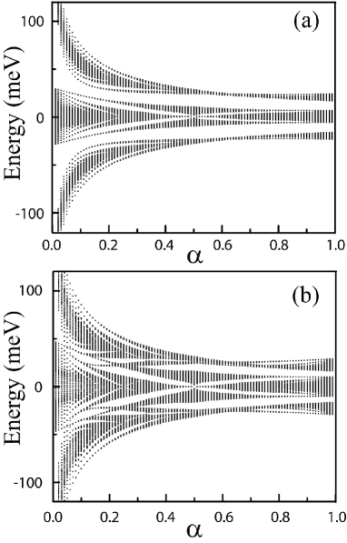
Figure 3: Single-electron energy spectra of graphene monolayer in a periodic potential and an external magnetic field. The period of the potential is $a_{0}=20$ nm and its amplitude is (a) $V_{0}=50$ meV and (b) $V_{0}=100$ meV. The energy spectra are shown as a function of the parameter $\alpha=\Phi_{0}/\Phi$.

The eigenfunctions of the Hamiltonian (13), corresponding to the LL with index $n$, are given by

$$\Psi_{n,k}=C_{n}\left(\begin{array}[]{c}s_{n}i^{|n|-1}\phi_{|n|-1,k}\\ i^{|n|}\phi_{|n|,k}\end{array}\right),$$ (15)

where $C_{n}=1$ for $n=0$ and $C_{n}=1/\sqrt{2}$ for $n\neq 0$. Here $\phi_{n,k}$ is the Landau wave function introduced by Eq. (8) for an electron with parabolic dispersion relation. The graphene monolayer is then placed in a weak periodic potential $V(x,y)$, which is given by Eq. (9). This potential introduces coupling of LLs in graphene. The corresponding matrix elements of the periodic potential are

$$\left\langle n^{\prime}k^{\prime}\right|\cos(q_{0}y)\left|nk\right\rangle=$$

$$\frac{i^{n-n^{\prime}}}{2}C_{n}C_{n^{\prime}}\left\{\delta_{k^{\prime},k+q_{0}}+(-1)^{n-n^{\prime}}\delta_{k^{\prime},k-q_{0}}\right\}\times$$

$$\left[s_{n}s_{n^{\prime}}M_{|n^{\prime}|-1,|n|-1}+M_{|n^{\prime}|,|n|}\right]$$ (16)

and

$$\left\langle n^{\prime}k^{\prime}\right|\cos(q_{0}x)\left|nk\right\rangle=\frac{\delta_{k^{\prime},k}}{2}C_{n}C_{n^{\prime}}e^{-iq_{0}k\ell_{0}^{2}}$$ (17)

$$\times\left[1+(-1)^{n-n^{\prime}}\right]\left[s_{n}s_{n^{\prime}}M_{|n^{\prime}|-1,|n|-1}+M_{|n^{\prime}|,|n|}\right].$$

For a given LL with index $n$, the periodic potential is determined by the effective value

$$V_{0}\left[s_{n}^{2}M_{|n|-1,|n|-1}+M_{|n|,|n|}\right]$$

$$\propto V_{0}\left[s_{n}^{2}L_{|n|-1}(\pi\alpha)+L_{|n|}(\pi\alpha)\right].$$ (18)

The flatbands in graphene are therefore realized at points where $s_{n}^{2}L_{|n|-1}(\pi\alpha)+L_{|n|}(\pi\alpha)$ is 0. For $n=0$, i.e., $s_{0}=0$, this is exactly the same condition as in conventional system, but for other LLs the condition of flatbands becomes $L_{|n|-1}(\pi\alpha)+L_{|n|}(\pi\alpha)=0$.

In Fig. 3 the Hofstadter butterfly energy spectra is shown for a graphene monolayer, taking into account three LLs with $n=-1$, 0, and 1. The main difference between the conventional systems and graphene is the broadening of the energy structure within a single LL. For conventional system [Fig. 2], the width of the energy spectra for the $n=1$ LL is small for small values of $\alpha$ and large for large $\alpha$. In graphene the behavior is different: the broadening of the $n=1$ LL is large for small values of $\alpha$ and small for intermediate and large values of $\alpha$. Another specific feature of the energy spectra of graphene is that the mixing of the LLs, introduced by the periodic potential, is visible for much large values of the amplitude of the potential, $V_{0}\approx 100$ meV compared to $V_{0}\approx 20$ meV in conventional systems [Fig. 2(b)].

IV.2 Moiré structure

With the system of graphene one has the unique possibility to generate in the Hamiltonian a periodical perturbation (periodic potential) based on the intrinsic structure of graphene-based systems. Such a periodic structure is based on the Moiré pattern which appears between two similar regular structures overlaid at an angle. In graphene, the Moiré pattern is realized in (i) twisted bilayer graphene stacking_geometry_06 ; bilayer_with_twist_07 ; misoriented ; multi_layer_08 ; quantum_interference_08 ; Van_hove_twisted_10 ; Mele_moire_2010 ; trasport_twisted_graphene ; bistritzer ; luican which consists of two monolayers with relative small rotation angle between the layers; (ii) graphene monolayer on hexagonal boron nitride substrate with rotational misalignment between the graphene monolayer and the h-BN hbn ; zero_energy_mode ; graphene_moire_parten ; dean_13 ; hunt_13 ; geim_13 . Realization of the Moiré pattern in two hexagonal lattices (layers) is shown in Fig. 4. That pattern introduces a large-scale periodicity in the Hamiltonian of the systems, which, in a magnetic field, results in the Hofstadter butterfly spectra.

For twisted bilayer graphene the periodical modulation of the Hamiltonian is introduced through the interlayer hopping coupling which capture the periodic structure of the Moiré pattern. The interlayer coupling matrix is bistritzer

$$T(\vec{r})=w\sum_{j}e^{-i\vec{q}_{j}\vec{r}}T_{j},$$ (19)

where $j=1,2,3$ and matrices $T_{j}$ have the form

$$T_{1}=\left(\begin{array}[]{cc}1&1\\ 1&1\end{array}\right),\,T_{2}=\left(\begin{array}[]{cc}e^{-i\psi}&1\\ e^{i\psi}&e^{-i\psi}\end{array}\right),\,T_{3}=\left(\begin{array}[]{cc}e^{i\psi}&1\\ e^{-i\psi}&e^{i\psi}\end{array}\right).$$ (20)

Here $\psi=2\pi/3$, $\vec{q}_{1}=k_{D}\theta(0,-1)$, $\vec{q}_{2}=k_{D}\theta(\sqrt{3}/2,1/2)$, $\vec{q}_{3}=k_{D}\theta(-\sqrt{3}/2,1/2)$, $\theta$ is the twist angle, $k_{D}$ is the Dirac momentum, and $w$ is the hopping energy. The interlayer coupling has a matrix form, where the two components of the matrix correspond to two layers of graphene bilayer.

Figure 4: Moiré pattern in two hexagonal lattices with rotational misalignment. The two lattices, which correspond to two layers are shown by red and black dots, respectively.

The Moiré periodicity in the matrix $T(\vec{r})$ results in the formation of the Hofstadter butterfly pattern, which was studied in Refs. bistritzer as a splitting of the Landau levels due to the weak periodical modulation of $T(\vec{r})$. Since the area of the Moiré units cell is $\propto 1/\theta^{2}$, to observe the Hofstadter butterfly pattern for experimentally realized magnetic fields the twist angle should be small, $\theta\lesssim 5^{0}$.

Just as for the twisted bilayer graphene, the periodical perturbation in the Hamiltonian of monolayer graphene placed on a h-BN substrate is introduced through the periodical modulation of the interlayer coupling. The difference from the bilayer graphene case is that there is a small $\approx 1.8$% lattice mismatch between graphene and the BN. As a result, the interlayer coupling is determined by both the lattice mismatch and rotational misalignment by an angle $\theta$. Then the corresponding superlattice period $a_{0}$ depends both on the twist angle and the lattice mismatch. Even in the case of perfect alignment, i.e., for the zero twist angle, the superlattice period is $a_{0}\approx 13$ nm. This value introduces upper limits on the superlattice period. This is different from twisted graphene bilayer, for which there is no superllatice for perfect alignment of the layers and there is no constraint on the values of $a_{0}$. Another specific feature of graphene monolayer on the h-BN substrate is an asymmetry term in the effective Hamiltonian of graphene, which is due to different couplings of the B and N atoms to the graphene layer.

The periodic perturbation of the graphene Hamiltonian on the h-BN substrate, i.e., the graphene superlattice, results in the formation of multiple Moiré minibands and generation of secondary Dirac points zero_energy_mode ; graphene_moire_parten ; Dirac_edges_graphene_moire near the edges of the superlattice Brillouin zone. These points are characterized by the wave vector $G=4\pi/\sqrt{3}a_{0}$. The energy corresponding to this vector is $E_{G}=\hbar v_{F}G/2$. To observe these secondary Dirac points the graphene should be doped upto energy $E_{G}$. Since the period of the Moiré superlattice is determined by the twist angle, the doping requirement introduces a constraint on the values of the twist angle, which should be less than $1^{0}$ geim_13 . The formation of the fractal Hofstadter butterfly pattern in graphene on the h-BN substrate was studied theoretically in Ref. Dirac_edges_graphene_moire and was later observed experimentally in Refs. hunt_13 ; dean_13 ; geim_13 . This butterfly pattern was realized as splitting of the Moiré minibands (secondary Dirac cones) by a magnetic field. An example of the experimental results from the magnetoconductance probe of the minigap opening in graphene is shown in Fig. 5, where the fractal pattern is clearly visible.

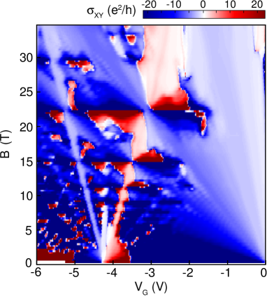
Figure 5: Experimental results for the Hall conductance probe of minigap opening within a Landau level in graphene, depicting the self-similarity pattern. (Courtesy of P. Kim and C. Dean).

V Bilayer graphene

Bilayer graphene consists of two coupled monolayers. This coupling opens a gap in the low energy dispersion relation and, in a magnetic field, modifies the LL structure. We consider the bilayer graphene with Bernal stacking. A single-particle Hamiltonian (kinetic energy part) of this system in a magnetic field is mccann_06

$${\cal H}_{\xi}^{(bi)}=\xi\left(\begin{array}[]{cccc}\frac{U}{2}&v_{\rm F}\pi_{-}&0&0\\ v_{\rm F}\pi_{+}&\frac{U}{2}&\xi\gamma_{1}&0\\ 0&\xi\gamma_{1}&-\frac{U}{2}&v_{\rm F}\pi_{-}\\ 0&0&v_{\rm F}\pi_{+}&-\frac{U}{2}\end{array}\right),$$ (21)

where $\xi=\pm 1$ corresponds to two valley ($K$ and $K^{\prime}$), $U$ is the inter-layer bias voltage which can be varied for a given system, and $\gamma_{1}\approx 0.4$ eV is the inter-layer coupling. The eigenfunctions of the Hamiltonian (21) can be expressed in term of the Landau functions $\phi_{n,k}$ [Eq. (8)]

$$\Psi^{\rm(bi)}_{n,k}=\left(\begin{array}[]{c}\xi C_{1}\phi_{|n|-1,k}\\ {\rm i}C_{2}\phi_{|n|,k}\\ {\rm i}C_{3}\phi_{|n|k}\\ \xi C_{4}\phi_{|n|+1,k}\end{array}\right),$$ (22)

where the coefficients, $C_{1}$, $C_{2}$, $C_{3}$, and $C_{4}$, can be found from the following system of equations

$$\varepsilon C_{1}=\xi uC_{1}-\sqrt{n}C_{2}$$ (23)

$$\varepsilon C_{2}=\xi uC_{2}-\sqrt{n}C_{1}+\tilde{\gamma}_{1}C_{3}$$ (24)

$$\varepsilon C_{3}=-\xi uC_{3}+\sqrt{n+1}C_{4}+\tilde{\gamma}_{1}C_{2}$$ (25)

$$\varepsilon C_{4}=-\xi uC_{4}+\sqrt{n+1}C_{3}.$$ (26)

Here all energies are expressed in units of $\epsilon_{B}=\hbar v_{\rm F}/\ell_{0}$, $\varepsilon$ is the energy of the LL, $u=U/(2\epsilon_{B})$, and $\tilde{\gamma}_{1}=\gamma_{1}/\epsilon_{B}$.

The energy spectra of the LLs can be found from pereira_07

$$\left[\left(\varepsilon+\xi u\right)^{2}-2n\right]\left[\left(\varepsilon-\xi u\right)^{2}-2(n+1)\right]=\tilde{\gamma}_{1}^{2}\left[\varepsilon^{2}-u^{2}\right].$$ (27)

For each value of $n\geq 0$ there are four solutions of the eigenvalue equation (27), corresponding to four Landau levels in a bilayer graphene for a given valley, $\xi=\pm 1$. For zero bias voltage, $U=0$ these four Landau levels are

$$\epsilon=\pm\sqrt{2n+1+\frac{\tilde{\gamma}^{2}_{1}}{2}\pm\frac{1}{2}\sqrt{(2+\tilde{\gamma}^{2}_{1})^{2}+8n\tilde{\gamma}^{2}_{1}}}.$$ (28)

In this case each Landau level has two-fold valley degeneracy which is lifted at finite bias voltage $U$.

For $n=0$ there are two special LLs of bilayer graphene. One LL has the energy $\varepsilon=-\xi u$ and the wave function of this LL consists of $\phi_{0,k}$ functions only

$$\Psi^{\rm(bi)}_{0_{1},k}=\left(\begin{array}[]{c}\phi_{0,k}\\ 0\\ 0\\ 0\end{array}\right).$$ (29)

This LL of bilayer graphene has exactly the same properties as for the $0$-th conventional, non-relativistic Landau level. For zero bias voltage $U$, this level has zero energy.

For small values of $U$ there is another solution of Eq. (27) with $n=0$, which has almost zero energy, $\varepsilon\approx 0$. The corresponding LL has the wavefunction

$$\Psi^{\rm(bi)}_{0_{2},k}=\frac{1}{\sqrt{\gamma_{1}^{2}+2\epsilon_{B}^{2}}}\left(\begin{array}[]{c}\gamma_{1}\phi_{1,k}\\ 0\\ \sqrt{2}\epsilon_{B}\phi_{0,k}\\ 0\end{array}\right).$$ (30)

The wave function of this LL is the mixture of the $n=0$ and $n=1$ conventional (nonrelativistic) Landau functions $\phi_{0,k}$ and $\phi_{1,k}$. This mixing depends on the magnitude of the magnetic field. In a small magnetic field, $\epsilon_{B}\ll\gamma_{1}$, the wavefunction is $(\psi_{1,m},0,0,0)^{T}$ and the LL is identical to the $n=1$ non-relativistic LL. In a large magnetic field $\epsilon_{B}\gg\gamma_{1}$, the LL wavefunction is $(0,0,\psi_{0,m},0)^{T}$ and the bilayer LL has the same properties as the $n=0$ non-relativistic LL.

Following the same procedure as for the conventional systems and the graphene monolayer, we can find the matrix elements of the periodic potential in the basis of LL wave function of bilayer graphene

$$\left\langle n^{\prime}k^{\prime}\right|\cos(q_{0}y)\left|nk\right\rangle=$$

$$\frac{i^{n-n^{\prime}}}{2}C_{n}C_{n^{\prime}}\left\{\delta_{k^{\prime},k+q_{0}}+(-1)^{n-n^{\prime}}\delta_{k^{\prime},k-q_{0}}\right\}$$

$$\times\left[C_{n,1}C_{n^{\prime},1}M_{|n^{\prime}|-1,|n|-1}+C_{n,4}C_{n^{\prime},4}M_{|n^{\prime}|+1,|n|+1}\right.$$

$$+\left.\left(C_{n,2}C_{n^{\prime},2}+C_{n,3}C_{n^{\prime},3}\right)M_{|n^{\prime}|,|n|}\right]$$ (31)

and

$$\left\langle n^{\prime}k^{\prime}\right|\cos(q_{0}x)\left|nk\right\rangle=\frac{\delta_{k^{\prime},k}}{2}C_{n}C_{n^{\prime}}e^{-iq_{0}k\ell_{0}^{2}}\left[1+(-1)^{n-n^{\prime}}\right]$$

$$\times\left[C_{n,1}C_{n^{\prime},1}M_{|n^{\prime}|-1,|n|-1}+C_{n,4}C_{n^{\prime},4}M_{|n^{\prime}|+1,|n|+1}\right.$$

$$+\left.\left(C_{n,2}C_{n^{\prime},2}+C_{n,3}C_{n^{\prime},3}\right)M_{|n^{\prime}|,|n|}\right].$$ (32)

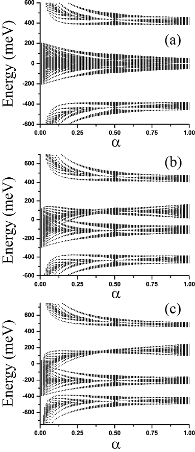
Figure 6: Single-electron energy spectra of bilayer graphene in a periodic potential and an external magnetic field. The period of the potential is $a_{0}=20$ nm and its amplitude is $V_{0}=100$ meV. The bias voltage is (a) $U=0$, (b) $U=200$ meV, and (c) $U=400$ meV. The energy spectra are shown as a function of the parameter $\alpha=\Phi_{0}/\Phi$.

With the known matrix elements of the periodic potential, we can find the energy spectra of bilayer graphene in a magnetic field and weak (or intermediate) periodic potential, taking into account many LLs. The results are shown in Fig. 6. For zero bias voltage [Fig. 6(a)], similar to graphene, the inter-Landau level coupling becomes important only for large amplitudes of the periodic potential, $V_{0}>100$ meV. This is true except for two degenerate LLs of type (29) and (30), for which the inter-level coupling becomes strong even for small amplitudes $V_{0}$ due to the degeneracy of the levels. In this case, the structure of the energy spectrum near zero energy becomes complicated due to the mixture of two degenerate butterfly structures. These two butterfly structures are not identical due to different types of wave functions of the two LLs and correspondingly different effective periodic potentials. For one LL the effective periodic potential is $V_{0}L_{0}(\pi\alpha)$, while for the other LL, the wave function of which is given by Eq. (30), the effective strength of the potential is

$$\frac{V_{0}}{\gamma_{1}^{2}+2\epsilon_{B}^{2}}\left(\gamma_{1}^{2}L_{1}(\pi\alpha)+2\epsilon_{B}^{2}L_{0}(\gamma_{1}^{2}L_{0}(\pi\alpha)\right).$$ (33)

At a finite bias voltage [Fig. 6(b,c)] the degeneracy of two low energy LLs is lifted and we can observe two distinctively separated butterfly structures for large values of $\alpha$. For small $\alpha$ (large magnetic field), there is a large overlap of the two butterfly structures and a strong inter-level mixture is expected. In one of the initially degenerate LLs the flatband condition is satisfied for $\alpha\approx 0.35$ [Fig. 6(c)]. The Hofstadter butterfly in bilayer graphene has been studied in nemec , where general configuration of the bilayer graphene, e.g., continuous displacement between the layers, were introduced.

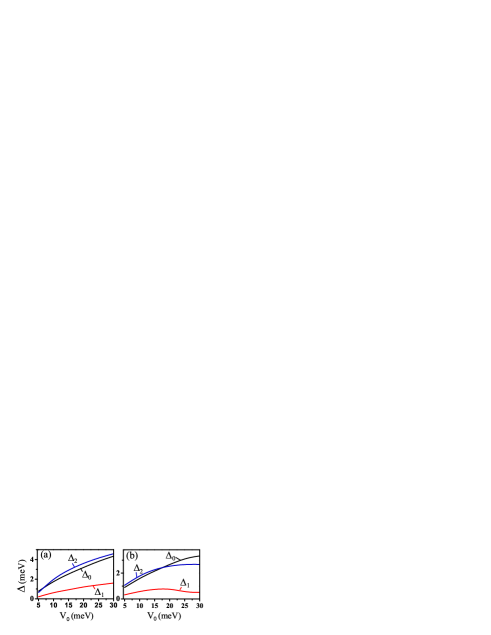
Figure 7: The band gaps in the $n=0$, $n=1$, and $n=2$ LLs versus the amplitude of the periodic potential, $V_{0}$, for interacting systems with half filling of the $n=0$ Landau level. The band gap $\Delta_{n}$ at LL with index $n$ is defined as the gap between the corresponding bands of Dirac fermions in a magnetic field corresponding to $\alpha=1/2$. The period of the potential is (a) $a_{0}=20$ nm and (b) $a_{0}=40$ nm.

VI Interaction effects

VI.1 Hartree approximation

Theoretical analysis of the Hofstadter butterfly problem was mainly restricted to noninteracting electron systems. There were only a few papers that reported on the effects of electron-electron interactions on the fractal energy spectra screening_95 ; vidar ; doh_salk ; Apalkov_14 The problem with inclusion of the electron-electron interaction into the system is related to the requirement that the system should have a large size to capture the fractal nature of the spectrum. The Hartree or mean-field approaches have been used to estimate the effect of interactions on the electron energy spectrum.

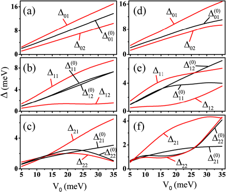
Figure 8: The band gaps versus $V_{0}$ for $n=0$ (a,d), $n=1$ (b,e), and $n=2$ (c,f) LLs. The band gaps are defined as the gaps between the corresponding bands of Dirac fermions in a magnetic field for $\alpha=1/3$. The black lines correspond to the case of the nonintercting system, while the red lines correspond to the Dirac fermions with Hartree interaction and half filling of the $n=0$ Landau level. The gaps are labeled as $\Delta^{(0)}_{ni}$ (noninteracting system) and $\Delta_{ni}$ (interacting system), where $n$ is the LL index and $i=1$ and $2$ corresponds to the low-energy and high energy gaps, respectively. The period of the periodic potential is $a_{0}=20$ nm (a,b,c) and $a_{0}=40$ nm (d,e,f).

In the Hartree approach the problem is reduced to the single-electron problem in a periodic potential and the Hartree potential, produced by the inter-electron interaction with average electron density. The Hamiltonian of the system with the Hartree interaction is

$${\cal H}={\cal H}_{0}(p_{x},p_{y})+V(x,y)+V_{H}(x,y),$$ (34)

where $V_{H}(x,y)$ is the Hartree potential, which can be expressed as

$$V_{H}(x,y)=\int dx_{1}dy_{1}\frac{e^{2}}{\kappa|\vec{r}-\vec{r}_{1}|}n(\vec{r}_{1}).$$ (35)

Here $\kappa$ is the background dielectric constant and

$$n(\vec{r})=\sum_{i}^{\prime}|\Psi_{i}(x,y)|^{2},$$ (36)

where the prime means that the sum goes over all occupied electron states. The number of occupied states is determined by the chemical potential of the system, $\mu$, i.e., only the states with energy $E_{i}$ less than the chemical potential, $E_{i}<\mu$, are occupied. The wave functions $\Psi_{i}(x,y)$ are single particle wave functions of Hamiltonian (34).

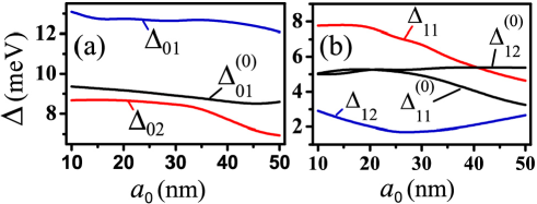
Figure 9: The band gaps in (a) $n=0$ and (b) $n=1$ LLs versus the period $a_{0}$ of the periodic potential for non-interacting system and the system with interaction and half filling of the $n=0$ Landau level for $\alpha=1/3$. The amplitude of the potential is $V_{0}=25$ meV.

The finite size system (34)-(36) can be solved numerically following the self-consistent procedure. The final solution is the energy spectrum of electron system with the Hartree interaction. It is convenient to express the Hartree potential in the reciprocal space. The electron density should have the same spatial symmetry as the periodic potential. Then the Fourier transform of the electron density

$$\tilde{n}(\vec{G})=\frac{1}{A_{0}}\int d\vec{r}\,n(\vec{r})e^{-i\vec{r}\vec{G}},$$ (37)

is nonzero only at points of reciprocal lattice, i.e., at points $\vec{G}=\vec{G}_{n_{x},n_{y}}=(2\pi/a_{0})(n_{x},n_{y})$, where $n_{x}$ and $n_{y}$ are integers. Here $A_{0}$ in Eq. (37) is the area of the sample. Then the Fourier transform of the Hartree potential is also nonzero only at points of the reciprocal lattice and is given by

$$V(\vec{G})=\frac{2\pi e^{2}}{\kappa|\vec{G}|}\tilde{n}(\vec{G})~{}~{}\mathrm{for}~{}~{}\vec{G}\neq 0,$$ (38)

and $V(\vec{G}=0)=0$. In Ref. screening_95 ; vidar this approach was used to study the interaction effects on Hofstadter butterfly in conventional systems, where strong oscillations of the LL bandwidth with chemical potential, i.e., filling of the LL, were reported.

Following the procedure outlined above, the interaction effects on the band structure of the Hofstadter butterfly in graphene were studied in Ref. Apalkov_14 . The graphene LLs with indices $n=0$, $n=\pm 1$, and $n=\pm 2$ were considered and the gap structure for $\alpha=1/2$ and $\alpha=1/3$ with interaction and without interaction were analyzed. Periodic boundary conditions were applied and the size of the system was $50a_{0}\times 50a_{0}$. For $\alpha=1/2$, the system is expected to have two bands separated by a gap. For noninteracting system the gap is zero at all LLs. Finite electron-electron interactions open gaps for $\alpha=1/2$, where the magnitude of the gap depends both on the period $a_{0}$ of the periodic potential and its magnitude $V_{0}$. In Fig. 7 Apalkov_14 this dependence is shown for the case when half of the $n=0$ LL is occupied, i.e., the chemical potential is zero. Strong nonmonotonic dependence of the gaps on the LL index is clearly visible in Fig. 7, and as a function of the LL index the gap has a minimum for $n=1$.

The case of $\alpha=1/3$ has been also studied in Ref. Apalkov_14 . In this case even without the interaction, the system has three bands and correspondingly two nonzero gaps in each LL. For a non-interacting system the two gaps $i=1,2$ in the LL with index $n$ are labeled as $\Delta^{(0)}_{n,i}$. Due to the symmetry the two gaps in the $n=0$ LL are the same, $\Delta^{(0)}_{01}=\Delta^{(0)}_{02}$. In higher LLs ($n=1$ and 2) the two gaps are different due to the LL mixing introduced by the periodic potential. Then the gaps in the same LL are different, e.g., $\Delta^{(0)}_{11}\neq\Delta^{(0)}_{12}$. Interaction modifies the gaps with the general tendency that the lower energy gap is enhanced and the higher one is suppressed. For $n=0$ the two gaps are no longer equal, $\Delta_{01}\neq\Delta_{02}$. As a function of the amplitude of the periodic potential the gaps have nonmonotonic dependence with local minimum (or maximum) at finite values of $V_{0}$. The higher energy gap for $n=1$, $\Delta_{12}$, is strongly suppressed by the electron-electron interactions.

The enhancement or suppression of the gaps by the electron-electron interactions depend not only on the amplitude of the periodic potential but also on the period of the potential. This dependence is shown in Fig. 9 for $\alpha=1/3$ and amplitude of the potential $V_{0}=25$ meV. The results are shown for the $n=0$ and $n=1$ LLs only. The gaps, both for the system with interactions and without interactions, have weak dependence on $a_{0}$ for small values of the period, $a_{0}\lesssim 25$ nm. For larger values of $a_{0}$ there is a strong suppression of the low energy gap, $\Delta_{11}$, in the $n=1$ LL and higher energy gap, $\Delta_{02}$, in the $n=0$ LL. In general, the gaps have monotonic dependence on $a_{0}$, except the higher energy gap, $\Delta_{12}$, in the $n=1$ LL, which has a minimum at $a_{0}\approx 25$ nm.

VI.2 Correlation effects: Extreme quantum limit

In the extreme quantum limit, i.e., in a strong magnetic field and extremely low temperatures, electrons display the celebrated fractional quantum Hall effect (FQHE), which is an unique manifestation of the collective modes of the many-electron system. The effect is driven entirely by the electron correlations resulting in the so-called incompressible states FQHE_book ; laughlin . It should be pointed out that the properties of incompressible states of Dirac fermions have been established theoretically for monolayer graphene mono_FQHE and bilayer graphene bi_FQHE and the importance of interactions in the extreme quantum limit are well known chapter ; interaction . There are also experimental evidence of the FQHE states in graphene graphene_book ; FQHE_expt . The precise role of FQHE in the fractal butterfly spectrum has remained unanswered however. Interestingly, in a recent experiment geim_14 , the butterfly states in the integer quantum Hall regime vktc have been already explored. Understanding the effects of electron correlations on the Hofstadter butterfly is therefore a pressing issue. In Ref. butterfly_FQHE , the authors have recently developed the magnetic translation algebra mag_translation ; haldane_85 ; read of the FQHE states, in particular for the primary filling factor $\nu=\frac{1}{3}$ for Hofstadter butterflies in graphene butterfly_FQHE . They considered a system of electrons in a periodic rectangular geometry that was very useful earlier in studying the properties of the FQHE in the absence of a periodic potential prg . The work in Ref. butterfly_FQHE has unveiled a profound effect of the FQHE states on the butterfly spectrum resulting in a transition from the incompressible FQHE gap to the gap due to the periodic potential alone, as a function of the periodic potential strength. There are also crossing of the ground state and low-lying excited states depending on the number of flux quanta per unit cell, that are absent when the periodic potential is turned off.

The magnetic translation analysis was employed to study the effect of a periodic potential on the FQHE in graphene for the primary filling factor $\nu=1/3$. For $\alpha=1/2$ and $\alpha=1/3$, increasing the periodic potential strength $V_{0}$ resulted in a closure of the FQHE gap and the appearance of gaps due to the periodic potential butterfly_FQHE . It was also found that for $\alpha=1/2$ this results in a change of the ground state and consequently in the change of the ground state momentum. For $\alpha=1/3$, despite the observation of the crossing between the low-lying energy levels, the ground state does not change with an increase of $V_{0}$ and is always characterized by zero momentum. The difference between these two $\alpha$ s is a result of the origin of the gaps for the energy levels. For $\alpha=1/2$ the emergent gaps are due to the electron-electron interaction only, whereas for $\alpha=1/3$ these are both due to the non-interacting Hofstadter butterfly pattern and the electron-electron interaction.

VII concluding Remarks

It has been a while since the beautiful theoretical idea of the Hofstadter butterfly which encompasses the fractal geometry and electron dynamics in a magnetic field and periodic potentials was proposed and its eventual confirmation in real physical systems in recent years. The unusual properties of graphene described here actually helped in finding the exotic butterflies with their fractal pattern. In achieving this feat the experimentalists made tremendous progress in understanding and controlling the properties of graphene under various constraints, and creating the Moiré pattern by finding the right substances. Discovery of the fractal butterfly in graphene has opened up new directions of research, both in materials research, and in fundamental studies of two-dimensional electrons. Future experiments will undoubtedly be in the limit of strong electron correlations, thereby opening up the fertile field of many-body effects in Dirac materials.

The work has been supported by the Canada Research Chairs Program of the Government of Canada. We wish to thank Philip Kim and Cory Dean for sending us a copy of Fig. 5. The work of V.M.A. has been supported by the NSF grant ECCS-1308473.

References

- (1) Electronic address: Tapash.Chakraborty@umanitoba.ca
- (2) U. Rössler and M. Shurke, in Advances in Solid State Physics, edited by B. Kramer (Springer, Berlin 2000), Vol. 40, pp. 35-50.
- (3) P.G. Harper, Proc. Phys. Soc. London 68, 874 (1955).
- (4) D. Langbein, Phys. Rev. 180, 633 (1969).
- (5) D. Hofstadter, Phys. Rev. B 14, 2239 (1976).
- (6) Benoit B. Mandelbrot, The Fractal Geometry of Nature (W.H. Freeman and Company, New York, 1982).
- (7) M.C. Geisler, J.H. Smet, V. Umansky, K.von Klitzing, B. Naundorf, R. Ketzmerick, and H. Schweizer, Phys. Rev. Lett. 92, 256801 (2004).
- (8) M.C. Geisler, J.H. Smet, V. Umansky, K.von Klitzing, B. Naundorf, R. Ketzmerick, and H. Schweizer, Physica E 25, 227 (2004).
- (9) C. Albrecht, J.H. Smet, K. von Klitzing, D. Weiss, V.Umansky, and H. Schweitzer, Phys. Rev. Lett. 86, 147 (2001).
- (10) C. Albrecht, J.H. Smet, K. von Klitzing, D. Weiss, V.Umansky, and H. Schweitzer, Physica E 20, 143 (2003).
- (11) T. Schlösser, K. Ensslin, J.P. Kotthaus, and M. Holland, Europhys. Lett. 33, 683 (1996).
- (12) T. Schlösser, K. Ensslin, J.P. Kotthaus, and M. Holland, Semicond. Sci. Technol. 11, 1582 (1996).
- (13) U. Kuhl and H.-J. Stöckmann, Phys. Rev. Lett. 80, 3232 (1998).
- (14) M. Aidelsburger, M. Atala, M. Lohse, J.T. Barreiro, B. Paredes, and I. Bloch, Phys. Rev. Lett. 111, 185301 (2013).
- (15) H. Miyake, G.A. Siviloglu, C.J. Kennedy, W.C. Burton, and W. Ketterle, Phys. Rev. Lett. 111, 185302 (2013).
- (16) H. Aoki and M.S. Dresselhaus (Eds.), Physics of Graphene (Springer, New York 2014).
- (17) D.S.L. Abergel, V. Apalkov, J. Berashevich, K. Ziegler, and T. Chakraborty, Adv. Phys. 59, 261 (2010).
- (18) T. Chakraborty and V. Apalkov, in graphene_book Ch. 8; T. Chakraborty and V.M. Apalkov, Solid State Commun. 175, 123 (2013).
- (19) M. Xu, T. Liang, M. Shi, and H. Chen, Chem. Rev. 113, 3766 (2013).
- (20) C.R. Dean, L. Wang, P. Maher, C. Forsythe, F. Ghahari, Y. Gao, J. Katoch, M. Ishigami, P. Moon, M. Koshino, T. Taniguchi, K.Watanabe, K.L. Shepard, J.Hone, and P. Kim, Nature 497, 598 (2013).
- (21) B. Hunt, J.D. Sanchez-Yamagishi, A.F. Young, M. Yankowitz, B.J. LeRoy, K. Watanabe, T. Taniguchi, P. Moon, M. Koshino, P. Jarillo-Herrero, and R.C. Ashoori, Science 340, 1427 (2013).
- (22) L.A. Pomomarenko, R.V. Gorbachev, G.L. Yu, D.C. Elias, R. Jalil, A.A. Patel, A. Mishchenko, A.S. Mayorov, C.R. Woods, J.R. Wallbank, M. Mucha-Kruczynski, B.A. Piot, M. Potemski, I.V. Grigorieva, K.S. Novoselov, F. Guinea, V.I. Falko and A.K. Geim, Nature 497, 594 (2013).
- (23) C.R. Dean, A.F. Young, I. Meric, C. Lee, L. Wang, S. Sorgenfrei, K. Watanabe, T. Taniguchi, P. Kim, K.L. Shepard, J. Hone, J. Nat. nanotechnol. 5, 722 (2010).
- (24) R. Decker, Y. Wang, V.W. Brar, W. Regan, H.-Z. Tsai, Q. Wu, W. Gannett, A. Zettl, and M.F. Crommie, Nano Lett. 11, 2291 (2011).
- (25) J. Xue, J. Sanchez-Yamagishi, D. Bulmash, P. Jacquod, A. Deshpande, K. Watanabe, T. Taniguchi, P. Jarillo-Herrero, and B.J. LeRoy, Nat. Mater. 10, 282 (2011).
- (26) J.-W. Rhim and K. Park, Phys. Rev. B 86, 235411 (2012).
- (27) N. Nemec and G. Cuniberti, Phys. Rev. B 75, 201404 (2007);
- (28) O. Gat, and J.E. Avron, New J. Phys. 5, 44 (2003).
- (29) S. Janecek, M. Aichinger, and E.R. Hernandez, Phys. Rev. B 87, 235429 (2013).
- (30) S. Latil, and L. Henrard, Phys. Rev. Lett. 97, 036803 (2006).
- (31) J.M.B. Lopes dos Santos, N.M.R. Peres, and A.H. Castro Neto, Phys. Rev. Lett. 99, 256802 (2007).
- (32) V.M. Apalkov and T. Chakraborty, Phys. Rev. B 84, 033408 (2011).
- (33) J. Hass, F. Varchon, J.E. Millán-Otoya, M. Sprinkle, N. Sharma, W.A. de Heer, C. Berger, P.N. First, L. Magaud, and E.H. Conrad, Phys. Rev. Lett. 100, 125504 (2008).
- (34) S. Shallcross, S. Sharma and O.A. Pankratov, Phys. Rev. Lett. 101, 056803 (2008).
- (35) G. Li, Guohong, A. Luican, J.M.B. Lopes dos Santos, A.H. Castro Neto, A. Reina, J. Kong, and E.Y. Andrei, Nat. Phys. 6, 109 (2010).
- (36) E.J. Mele, Phys. Rev. B 8l, 161405 (2010).
- (37) R. Bistritzer and A.H. MacDonald, Phys. Rev. B 8l, 245412 (2010).
- (38) R. Bistritzer and A.H. MacDonald, Phys. Rev. B 84, 035440 (2011).
- (39) A. Luican, G. Li, A. Reina, J. Kong, R.R. Nair, K.S. Novoselov, A.K. Geim, and E.Y. Andrei, Phys. Rev. Lett. 106, 126802 (2011).
- (40) M. Kindermann, B. Uchoa, and D.L. Miller, Phys. Rev. B 86, 115415 (2012).
- (41) J.R. Wallbank, A.A. Patel, M. Mucha-Kruczynski, A.K. Geim and V.I. Fal’ko, Phys. Rev. B 87, 245408 (2013).
- (42) X. Chen, J.R. Wallbank, A.A. Patel, M. Mucha-Kruczynski, E. McCann and V.I. Fal’ko, Phys. Rev. B 89, 075401 (2014).
- (43) E. McCann, and V. Falko, Phys. Rev. Lett. 96 086805 (2006); E. McCann, Phys. Rev. B 74 161403 (2006).
- (44) J. Milton Pereira, F.M. Peeters, and P. Vasilopoulos, Phys. Rev. B 76, 115419 (2007).
- (45) Vidar Gudmundsson, and Rolf R. Gerhardts, Phys. Rev. B 52, 16744 (1995).
- (46) V. Gudmundsson and R.R. Gerhardts, Surf. Sci. 361-362, 505 (1996); Phys. Rev. B 52, 16744 (1995); Phys. Rev. B 54, 5223R (1996).
- (47) D. Pfannkuche and A.H. MacDonald, Phys. Rev. B 56, R7100 (1997); H. Doh and S.H. Salk, Phys. Rev. B 57, 1312 (1998).
- (48) V.M. Apalkov and T. Chakraborty, Phys. Rev. Lett. 112, 176401 (2014).
- (49) T. Chakraborty and P. Pietiläinen, The Quantum Hall Effects (Springer, New York 1995); T. Chakraborty, and P. Pietiläinen, The Fractional Quantum Hall Effect (Springer, New York 1988).
- (50) R.B. Laughlin, Phys. Rev. Lett. 50, 1395 (1983); Rev. Mod. Phys. 71, 863 (1999).
- (51) V.M. Apalkov and T. Chakraborty, Phys. Rev. Lett. 97, 126801 (2006).
- (52) V.M. Apalkov and T. Chakraborty, Phys. Rev. Lett. 105, 036801 (2010); V. Apalkov and T. Chakraborty, Phys. Rev. Lett. 107, 186803 (2011).
- (53) V. Apalkov and T. Chakraborty, Solid State Commun. 177, 128 (2014); D.S.L. Abergel and T. Chakraborty, Phys. Rev. Lett. 102, 056807 (2009); D. Abergel, V. Apalkov, and T. Chakraborty, Phys. Rev. B 78, 193405 (2008); D. Abergel, P. Pietiläinen, and T. Chakraborty, Phys. Rev.B 80, 081408 (2009); V. Apalkov and T. Chakraborty, Phys. Rev. B 86, 035401 (2012).
- (54) X. Du, I. Skachko, F. Duerr, A. Luican, and E.Y. Andrei, Nature 462. 192 (2009); D.A. Abanin, I. Skachko, X. Du, E.Y. Andrei, and L.S. Levitov, Phys. Rev. B 81, 115410 (2010); K.I. Bolotin, F. Ghahari, M.D. Shulman, H.L. Störmer, and P. Kim, Nature 462, 196 (2009); F. Ghahari, Y. Zhao, P. Cadden-Zimansky, K. Bolotin, and P. Kim, Phys. Rev. Lett. 106, 046801 (2011).
- (55) G.L. Yu, R.V. Gorbachev, J.S. Tu, A.V. Kretinin, Y. Cao, R. Jalil, F. Withers, L.A. Ponomarenko, B.A. Piot, M. Potemski, D.C. Elias, X. Chen, K. Watanabe, T. Taniguchi, I.V. Grigorieva, K.S. Novoselov, V.I. Falko, A.K. Geim, and A. Mishchenko, Nat. Phys. 10, 525 (2014).
- (56) K. von Klitzing and T. Chakraborty, Physics in Canada 67, 161 (2011).
- (57) J. Zak, Phys. Rev. 133, A1602 (1964); E. Brown, Phys. Rev. 133, A1038 (1964)
- (58) F.D.M. Haldane, Phys. Rev. Lett. 55, 2095 (1985).
- (59) A. Kol and N. Read, Phys. Rev. B 48, 8890 (1993).
- (60) A. Ghazaryan, T. Chakraborty, and P. Pietiläinen, arXiv: 1408.3424v1 (2014).
- (61) The periodic rectangular geomery was extensively used earlier in the study of the FQHE in various situations. For example, see T. Chakraborty, Surf. Sci. 229, 16 (1990); Adv. Phys. 49, 959 (2000); T. Chakraborty and P. Pietiläinen, Phys. Rev. Lett. 76, 4018 (1996); T. Chakraborty and P. Pietiläinen, Phys. Rev. B 39, 7971 (1989); V.M. Apalkov, T. Chakraborty, P. Pietiläinen, and K. Niemelä, Phys. Rev. Lett. 86, 1311 (2001); T. Chakraborty, P. Pietiläinen, and F.C. Zhang, Phys. Rev. Lett. 57, 130 (1986); T. Chakraborty and F.C. Zhang, Phys. Rev. B 29, 7032 (R) (1984); F.C. Zhang and T. Chakraborty, Phys. Rev. B 30, 7320 (R) (1984).