Random walks on stochastic hyperbolic half planar triangulations

Abstract

We study the simple random walk on stochastic hyperbolic half planar triangulations constructed in [3]. We show that almost surely the walker escapes the boundary of the map in positive speed and that the return probability to the starting point after $n$ steps scales like $\exp(-cn^{1/3})$.

1 Introduction

In this paper we study the behavior of the simple random walk on random half planar hyperbolic triangulations. The latter are probability measures on rooted half planar maps satisfying two natural properties, translation invariance and the domain Markov property. In [3] these measures were constructed and characterized as a one parameter family $\mathbb{H}_{\alpha}$ where $\alpha\in[0,1)$ is the probability that the face containing the root edge has an internal vertex. See further definitions below.

In [23] it is proved that the geometry of the map exhibits a phase transition at the value $\alpha=2/3$. When $\alpha<2/3$ the map almost surely has quadratic volume growth, infinitely many cut-sets of bounded size and the random walker is in the “Alexander-Orbach” regime, that is, after $t$ steps it is typically at distance $t^{1/3}$ (the same behavior as in random trees [17, 5] and in high-dimensional critical percolation [18]). When $\alpha>2/3$ the map is almost surely “hyperbolic” in the sense that it has exponential volume growth and positive anchored expansion. The hyperbolic regime is the focus of the current paper.

Since these maps are not sufficiently regular (namely, they are not transitive and have unbounded degrees) one cannot apply standard tools (such as [27]) to study basic properties the random walk such as its speed and return probabilities. Indeed, a special treatment, which employs the inherent randomness of the map, is needed. In this paper we show that in the hyperbolic phase $\alpha\in(2/3,1)$ the distance of the random walker from the boundary grows linearly (in particular, its speed is positive) and that the return probabilities follow a stretched exponential law $\exp(-cn^{1/3})$.

Theorem 1.1.

Fix $\alpha\in(2/3,1)$ and let $H$ be a random half planar triangulation with law $\mathbb{H}_{\alpha}$ with boundary $\partial H$. Consider the simple random walk $X_{n}$ on $H$ and write $d^{H}(x,y)$ for the graph distance between $x$ and $y$ in $H$. Then almost surely we have

$$\liminf_{n}\frac{d^{H}(X_{n},\partial H)}{n}>0.$$

Theorem 1.2.

Fix $\alpha\in(2/3,1)$. Given the map $H$ with law $\mathbb{H}_{\alpha}$, let $\mathbf{P}_{H}$ denote the law of a simple random walk on $H$ starting from $\rho$. There are positive constants $c,C$ depending only on $\alpha$ so that $\mathbb{H}_{\alpha}$-a.s. for all large enough $n$

$$e^{-Cn^{1/3}}\leq\mathbf{P}_{H}(X_{n}=\rho)\leq e^{-cn^{1/3}}.$$

1.1 Half planar maps

Recall that a planar map is a proper embedding (that is, with no crossing edges) of a connected (multi) graph on the sphere viewed up to orientation preserving homeomorphisms from the sphere to itself. Connected components of the complement of the embedding are called faces. We shall focus maps with a boundary, that is one face is marked as the external face and the edges and vertices incident to it form the boundary of the map. Vertices that are not on the boundary are called internal vertices. In this paper the boundary will always be simple, that is, the boundary edges and vertices form a simple cycle or a bi-infinite simple path. A triangulation is a map where every face has precisely three edges except possibly an external face. If the external face of a triangulation is a simple cycle with $p$-edges, we say it is a triangulation of a $p$-gon. Half planar triangulations are triangulations which are locally finite, one-ended (that is, the removal of any finite set of vertices results in precisely one infinite cluster) and have a bi-infinite simple boundary. In other words, these triangulations can be embedded such that the union of all vertices, edges and faces which are not the external face equals $\mathbb{R}\times\mathbb{R}_{+}$. All our maps are rooted, that is, an oriented edge is specified as the root. In a half planar map, the root is always on the boundary and is oriented in a way such that the external face is to the right of the root.

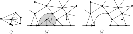
Figure 1: An illustration of domain Markov Property. Left: A finite simply connected map $Q$. Centre: A part of $M$ containing $Q$ with $2$ edges along the boundary. Right: The resulting map $\tilde{M}$ after removal of $Q$. Domain Markov property states that the law of $\tilde{M}$ is the same as that of $M$.

In [3], measures on half planar maps were considered which satisfy two natural properties: translation invariance and domain Markov property. See [3, Section 1.1] for the precise definitions. Roughly, the first property states that the law of the map is invariant to translation of the root edge along the boundary and the second states that if we condition that the map contains a fixed simply connected finite map which contains the root edge, then the law of the remaining map is the same. The latter is illustrated in Figure 1. The following theorem of [3] characterizes all such probability measures.

Theorem 1.3 ([3]).

All translation invariant and domain Markov measures supported on half planar triangulations without self-loops form a one parameter family $\mathbb{H}_{\alpha}$ where the parameter $\alpha\in[0,1)$. Furthermore $\alpha$ denotes the probability of the event that the triangle adjacent to the root edge is incident to an internal vertex.

1.2 About the proofs

Let us now give some brief intuition behind Theorems 1.1 and 1.2. It can be shown (see [20], Proposition 6.9) that graphs with positive Cheeger constant and at most exponential edge volume growth (meaning number of edges in the combinatorial ball of radius $r$ is at most $C^{r}$ for some $C>1$) has positive liminf speed. It can also be shown that on graphs with positive cheeger constant, the return probability is roughly $e^{-cn}$ for some $c>0$ (see (2.2)).

Our maps $H$ however are random and any given fixed configuration occurs somewhere in the map with probability $1$. Hence we need to consider a parameter more robust to such small perturbations called anchored expansion introduced by Benjamini, Lyons and Schramm [7]. Roughly, a graph has positive anchored expansion if, instead of all finite sets, all connected sets containing a fixed vertex in the graph have large boundary compared to its volume (details in Section 2.2). It was shown by Virág in [27] that graphs with anchored expansion and bounded degree has positive speed away from the root and the return probability is at most $\exp(-cn^{1/3})$ for some constant $c>0$ (for details see Section 2.2). Our maps $H$ do have anchored expansion almost surely as was illustrated in [23], Theorem 2.3. However, since the maps $H$ do not have uniform bounded degree, even positive speed away from the starting point in $H$ do not follow directly from Virág’s result in [27]. It is not difficult to obtain graphs with anchored expansion, exponential edge volume growth, unbounded degree and zero speed. However Theorem 3.5 of [24] does ensure that $H$ is transient almost surely just because $H$ has anchored expansion. Similar results for return probabilities on Cayley graphs were obtained in [26, 16].

Our proof methodology however relies on the techniques used by Virág in [27]. In [27], it was shown in Proposition 3.3 that every graph with anchored expansion contains a subgraph with positive Cheeger constant. The complement of this subgraph are sets with small boundary which Virág called islands. The trick is to control the distribution of these islands and make sure the walker does not spend too much time on the islands. We aim to follow a similar approach here and use the geometry of $H$ to arrive at the proposed results.

Recently a full-plane version of $H$ was constructed by Curien in [12]. Our second main tool is a coupling which realizes $H$ as a submap of its full plane version. Hence we can use the properties of random walk on the full-plane version to our advantage. For example, it was shown in [12] that random walk such full plane hyperbolic triangulations have positive speed almost surely.

Let us finish by mentioning that there has been growing interest in studying simple random walk on random planar maps in recent years (see [15, 9, 6, 8]). For example, it was an open question for about a decade whether uniform infinite planar triangulations given by [4] was recurrent or transient and only very recently it was resolved in [15]. However, many questions do remain open about the behaviour of simple random walk on the uniform infinite planar maps. For example, it is not known what is the speed of the simple random walk on these maps, and only an upper bound is provided in [6].

Disclaimer:

In the computations that follow, the constants might change from one line to next but we shall still denote them by the same letter $c$ for clarity. Also, we fix an $\alpha\in(2/3,1)$ throughout the rest of the paper and we shall drop the subscript $\alpha$ from the notation $\mathbb{H}_{\alpha}$ unless otherwise stated. Throughout, $H$ will denote a half plane map with law $\mathbb{H}$.

Organization:

In Sections 2.1 and 2.2 we recall some of the background results about expansion, anchored expansion and the paper of Virág [27]. In Sections 2.3, 2.4 and 2.5, we recall some of the results about the geometry of domain Markov triangulations, and derive some of their consequences. In Section 2.6, we recall the stochastic hyperbolic full plane triangulations of Curien [12] and prove the coupling of $\mathbb{H}$ as its sub-map. The knowledgeable reader could skim these and proceed to Section 3, where we prove Theorem 1.1 and Section 4 where we prove Theorem 1.2. We end with some comments and open questions in Section 5.

2 Background

We begin by reviewing various definitions we use. The reader familiar with anchored expansion and the work of Virág [27] may skip to Section 2.3. The reader familiar with the domain Markov property and [3] may skip Sections 2.3 and 2.4.

2.1 Graph notations and expansion

In this section we review the notion of expansion and some properties of graphs with positive Cheeger constant. Let us start with a few definitions. A weighted graph $G$ is a graph along with a positive weight $w(u,v)$ assigned to every edge $(u,v)$. The weight of a vertex $u$ is the sum of the weights of the edges incident to it and is denoted $w(u)$. We can view an unweighted graph also as a weighted graph with every edge having weight $1$. The random walk on a weighted graph is a Markov chain on its vertices with transition probabilities given by

$$p(x,y)=\frac{w(x,y)\mathbbm{1}_{x\sim y}}{w(x)}.$$

A sequence $(X_{n})$ in a graph $G$ is said to have positive liminf speed if

$$\liminf_{n\to\infty}\frac{d^{G}(X_{n},\rho)}{n}>0,$$

where $d^{G}$ denotes the graph distance, ignoring weights, and $\rho$ is some fixed vertex (this condition is clearly independent of $\rho$).

We consider the Hilbert space of functions defined on the vertices of $G$ with the inner product and norm

$$\langle f,g\rangle=\sum_{v\in V(G)}f(v)g(v)w(v),\quad\text{ and }\quad\|f\|=\langle f,f\rangle^{1/2}.$$

The Markov transition kernel $P$ for the random walk $\{X_{n}\}_{n\geq 1}$ on $G$ is the operator defined by $Pf(v)=\mathbb{E}(f(X_{1})|X_{0}=v)$.  For a set $S\subset V(G)$, the edge boundary of $S$, denoted $\partial S$ is defined to be the set of edges which have one endpoint in $S$ and the other in $V(G)\setminus S$. The Cheeger constant of $G$ is defined to be

$$i=i(G):=\inf_{S\subset V(G)}\frac{|\partial S|}{|S|}$$

where the infimum is over all finite subsets of vertices of $G$ and for any set $X$ of vertices or edges, $|X|$ denotes the sum of weights over $X$. Notice that the weight of a set of vertices $X$ in an unweighted graph is nothing but the sum of the degrees of the vertices in $X$.

Recall Cheeger’s classical inequality (see [13, 22, 20] or [27, Proposition 4.1]):

$$\|P\|\leq 1-\frac{i^{2}}{2}.$$ (2.1)

Inequality (2.1) implies

$$\mathbb{P}(X_{n}=\rho)=\frac{1}{w(\rho)}\langle\mathbbm{1}_{\rho},P^{n}\mathbbm{1}_{\rho}\rangle\leq\frac{1}{w(\rho)}\|\mathbbm{1}_{\rho}\|^{2}.\|P\|^{n}\leq(1-i^{2}/2)^{n}$$ (2.2)

Thus on a graph with positive Cheeger constant, the return probabilities decay exponentially in the number of random walk steps.

2.2 Anchored expansion

In the context of random graphs, frequently it is the case that expansion holds on average but not uniformly. In many such cases we have a weaker form knows as anchored expansion. We follow the terminology and reasoning of Virág [27], and repeat some definitions and results from there. We say a weighted graph $G$ has anchored expansion if $i^{*}(G)>0$, where the anchored expansion constant is defined by

$$i^{*}(G):=\liminf_{n\to\infty}\left\{\frac{|\partial S|}{|S|}\ :\ \text{$S\subset V(G)$ is connected, $|S|=n$ and $\rho\in S$}\right\}$$

As mentioned in the introduction, it was proved by Virág ([27]) that for bounded degree unweighted graphs, anchored expansion implies positive liminf speed. This result is not applicable in our setting because there is no uniform upper bounds on the degrees of the vertices of the graphs we consider. However, some information about the geometry of graphs with anchored expansion as established by Virág will be useful in our subsequent analysis. A key idea is to prove that a graph with anchored expansion contains a subgraph (called the ocean) with positive Cheeger constant. The complement of this subgraph has only finite components which Virág calls islands. The main idea of Virág was to show that the random walk cannot spend too much time in the islands.

For a finite set $S$ of vertices and a number $i\in(0,1)$, define the $i$-isolation of a finite set $S$ to be

$$\Delta_{i}S=i|S|-|\partial S|$$

A set of vertices with positive $i$-isolation is called $i$-isolated. A finite vertex set $S$ is called an $i$-isolated core if $\Delta_{i}S>\Delta_{i}A$ for every $A\subsetneq S$. Putting $A$ to be the empty set, we see that an $i$-isolated core is always $i$-isolated.

Proposition 2.1 ([27, Corollary 3.2]).

The union of finitely many $i$-isolated cores is an $i$-isolated core.

Suppose $0<i<i^{*}(G)$ and let $A_{i}$ be the union of all $i$-isolated cores in $G$. Anchored expansion and Proposition 2.1 imply that $i$-isolated cores containing any vertex have a bounded size, and so all connected components of $A_{i}$ are finite unions of $i$-isolated cores and hence are finite. The connected components of $A_{i}$ are called $i$-islands. Components of the complement $G\setminus A_{i}$ are called $i$-oceans (note $G\setminus A_{i}$ is not necessarily connected, since cutsets need not be connected). The following proposition shows that if $i^{\prime}<i$ and $G$ is an unweighted graph, all small $i$-islands “sink” in the $i^{\prime}$-ocean.

Proposition 2.2 ([27, Lemma 3.4]).

Suppose $G$ is an unweighted graph and $0<i^{\prime}<i<i^{*}(G)$. Then $A_{i^{\prime}}\subset A_{i}$. Further if $B$ is an $i$-island of size at most $1/i^{\prime}$. Then $B\subset G\setminus A_{i^{\prime}}$

We now describe an induced random walk. Let $\{X_{n}\}_{n\geq 1}$ be a random walk on a graph $G$ and suppose $0<i<i^{*}(G)$. Let $(\tau_{j})_{j\geq 0}$ be the ordered set of times at which $X_{t}$ is in an $i$-ocean. Then $(X_{\tau_{j}})$ is a reversible Markov chain on $G\setminus A_{i}$, and in particular is equivalent to a random walk on a graph $G_{i}$, which is closely related to the oceans, defined as follows. The vertices of $G_{i}$ are $G\setminus A_{i}$. For any vertex $v$, its weight $w_{i}(v)=w(v)$ is inherited from $G$. For any pair of vertices $u,v$, put a weight

$$w_{i}(u,v)=w_{i}(u)\mathbb{P}(X_{\tau_{1}}=v|X_{0}=u)$$

Note that $w_{i}$ is a symmetric function on the edges because of the reversibility of the walk. The following is proved in [27], following Lemma 3.4.

Proposition 2.3 ([27]).

The graph $G^{i}$ has cheeger constant at least $i$.

We say a graph $G$ has upper exponential growth if $|B_{r}|\leq e^{Cr}$ for some $C<\infty$, where $B_{r}=\{x:d^{G}(x,\rho)\leq r\}$ is the ball. As usual, this does not depend on the choice of $\rho$. This is connected to the random walk behaviour through the following:

Proposition 2.4.

Let $G$ be a graph with anchored expansion and upper exponential growth. Fix $i<i^{*}(G)$ and let $(\tau_{m})$ be as above. Then

$$\liminf_{m\to\infty}\frac{d^{G}(X_{\tau_{m}},\rho)}{m}>0$$

Proof.

This is a straightforward application of Lemma 4.2 of [27] to $G_{i}$, with $f(x)=d^{G}(x,\rho)$ (as opposed to the distance in $G_{i}$). ∎

2.3 Domain Markov triangulations

We now recall some definitions and properties of domain Markov half planar triangulations, which are the main object in this paper. We refer the reader to [3] for further details.

As mentioned in Theorem 1.3, $\alpha$ is the probability under $\mathbb{H}_{\alpha}$ of the event that the triangle incident to the any given boundary edge contains the edge and one internal vertex. The other possibilities are referred to as steps of the form $(L,i)$ or $(R,i)$. A step of form $(L,i)$ (resp. $(R_{i})$), is the event that the triangle incident to some fixed boundary edge has its third vertex on the boundary at a distance $i$ to the left (resp. right) of the given edge along the boundary (see Figure 2). We shall also talk about such events with the root edge replaced any fixed edge on the boundary of the map.

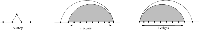
Figure 2: Left: An $\alpha$-step. Centre: A step of the form $(R,i)$. Right: A step of the form $(L,i)$. The gray area denotes some unspecified triangulation.

Because of translation invariance, the measures of such events do not depend on the choice of the boundary edge. It was also shown in [3] that for any fixed $i\geq 1$, the probability of $(L,i)$ and $(R,i)$ are the same (denoted $p_{i}$). Let $p_{i,k}$ denote the probability of the event that $(L,i)$ (or $(R,i)$) occurs and the triangle incident to the root edge separates $k$ internal vertices from infinity. Let $\beta=p_{1,0}$ be the probability of the event of the form $(R,1)$ with no internal vertex in the $2$-gon enclosed by the triangle incident to the root edge. The following formulas were derived in [3]:

$$\beta =\frac{\alpha(1-\alpha)}{2} p_{i,k} =\phi_{k,i+1}\beta^{i}(\alpha\beta)^{k} p_{i} \sim c\left(\frac{2}{\alpha}-2\right)^{i}i^{-3/2}$$ (2.3)

for some constant $c>0$, where $\phi_{k,i+1}$ denotes the number of triangulations of an $(i+1)$-gon with $k$ internal vertices. Notice that $p_{i}$ has an exponential tail for any $\alpha>2/3$.

2.4 Peeling

Let us briefly describe the concept of peeling, originating in work of Watabiki [28] and which was introduced in its present form in [1]. For further background, history and numerous applications of this very useful tool, we refer to [1, 2, 11, 21, 3, 6].

Given a map $T$, the idea is to construct a growing sequence of simply connected sub-maps $P_{n}$ with complements $T_{n}=T\setminus P_{n}$ as follows: at every step, we pick an edge in the boundary of $T_{n}$. We then construct $P_{n+1}$ by adding to $P_{n}$ the face $f$ of $T_{n}$ incident to the chosen edge along with any finite components of $T\setminus(P_{n}\cup f)$. This can be carried out for full plane maps, half plane maps, and other topologies as well.

If $T$ is a domain Markov half plane triangulation with law $\mathbb{H}$ and the edge chosen at each step is independent of $T_{n}$, then $T_{n}$ has the same law $\mathbb{H}$ for all $n$, and is independent of the revealed map $P_{n}$. Notice that every peeling step is of the form $(L,i)$ or $(R,i)$ as discussed in Section 2.3 and if $T$ is a full-plane map and $P_{n}$ is a triangulation of a $p$-gon, then necessarily $i\leq p-2$ since we do not allow self-loops in our triangulation.

The nice thing about peeling is that we are free to choose the edge on which we perform the next peeling step, the only constraint being the choice should depend only upon $P_{n}$ (along with possibly another source of randomness). We discuss two such algorithms which we shall need.

Peeling to reveal hulls:

The aim of this algorithm is to sequentially reveal the graph distance balls of radius $r$ around the root (or any finite subset of the boundary) along with the finite components of the complement. The hull of the ball of radius $r$ is completed at some random time $N_{r}$. Having obtained $P_{N_{r}}$, we peel continuously on the edges incident to vertices on the boundary of $P_{N_{r}}$ which is common with $T_{N_{r}}$ until every vertex on the boundary of $P_{N_{r}}$ is no longer in the boundary. We refer to [23], Section 4.1 for more details.

Peeling along random walk:

This was introduced in [6]. The idea is to run a random walk simultaneously with the peeling procedure. Having known $P_{n}$ and the vertex $v$ the random walker is in, there are two possible steps. If $v$ not in the boundary of $P_{n}$, we just perform a random walk step. Otherwise we continue peeling until we reveal the hull of the ball of radius $1$ around $v$ in $T_{n}$. Then we perform a random walk step. For details we refer to [6], Section 1.4.

2.4.1 Free triangulations

If we perform peeling steps in $H$, then it turns out via the calculations done in [3] that the finite triangulation enclosed by the revealed triangle after a step of the form $(L,i)$ or $(R,i)$ is distributed as a free triangulation (defined below) of an $(i+1)$-gon with parameter $\alpha\beta$ with $\beta$ given by (2.3). For details we refer to [1, 23].

Definition 2.5.

The free distribution on rooted triangulations of an $m$-gon with parameter $q\leq\frac{2}{27}$ is the probability measure that assigns weight $q^{n}/Z_{m}(q)$ to each rooted triangulation of the $m$-gon having $n$ internal vertices, where

$$Z_{m}(q)=\sum_{n}\phi_{n,m}q^{n}.$$

and $\phi_{n,m}$ is the number of triangulations of an $m$-gon with $n$ internal vertices.

The partition function in Definition 2.5 can be explicitly computed:

Proposition 2.6 ([14]).

Let $q=\theta(1-2\theta)^{2}$. Then for $m\geq 0$, $Z_{m+2}(q)$ is finite if and only if $q\in[0,2/27]$ (equivalently $\theta\in[0,1/6]$) and is given by

$$Z_{m+2}(q)=((1-6\theta)m+2-6\theta)\frac{(2m)!}{m!(m+2)!}(1-2\theta)^{-(2m+2)}.$$

Let $Y=0$ with probability $\alpha$ and $Y=i$ with probability $p_{i}$ (as given in (2.3)) for $i\geq 2$. Let $I_{m}$ be the number of internal vertices of a free triangulation of an $m$-gon with parameter $\alpha\beta$ for $m\geq 2$ and $I_{1}=1$. We say a variable $X$ has exponential tail if there exists a constant $c>0$ such that $\mathbb{P}(|X|>i)<e^{-ci}$. We next show that $Y+I_{Y+1}$ has exponential tail.

Lemma 2.7.

Let $Y,I_{Y+1}$ be as above. There exists a $\lambda>0$ such that

$$\mathbb{E}\left(e^{\lambda(Y+I_{Y+1})}\right)<\infty$$

In particular, the number of edges added in each peeling step has exponential tail.

Proof.

In light of (2.3), we need to show

$$\sum_{i\geq 1}e^{\lambda i}\beta^{i}\sum_{k\geq 0}e^{\lambda k}\phi_{i+1,k}(\alpha\beta)^{k}<\infty$$ (2.4)

But $\alpha\beta<2/27$ if $\alpha\in(2/3,1)$ via (2.3). Hence the sum over $k$ is finite if $\lambda>0$ is small enough via Proposition 2.6. Also since $\beta<1/9$,

$$\sum_{i\geq 1}e^{\lambda i}\beta^{i}Z_{i+1}(e^{\lambda}\alpha\beta)$$

is also finite for small enough choice of $\lambda$ via the expression of the partition function given by Proposition 2.6. The last sentence in the lemma follows from the fact that the number of edges added in each peeling step is dominated by $2Y+3I_{Y+1}-1$ via Euler’s formula. ∎

2.5 Geometry of supercritical triangulations

Here we restate some results from [23, 3] where the supercritical half planar triangulations were introduced and studied. We start with a statement about the probability of finite events in $\mathbb{H}_{\alpha}$, which could also be used as an alternative definition of $\mathbb{H}_{\alpha}$.

Lemma 2.8 ([3]).

Let $Q$ be a simply connected triangulation with a simple boundary, with some marked connected segment of $\partial Q$. Let $H$ be a half plane triangulation, and consider the event $A_{Q}$ that $Q$ is a sub-map of $H$ with the marked segment being the only intersection of $Q$ with $\partial H$. Then

$$\mathbb{H}(A_{Q})=\alpha^{V(Q)}\beta^{F(Q)-V(Q)}$$

where $V(Q)$ is the number of vertices of $Q$ not on $\partial H$ and $F(Q)$ is the number of faces of $Q$.

Recall the definition of $i$-isolated sets from Section 2.2: a set $S$ is $i$-isolated if $i|S|-|\partial S|$ is positive.

Lemma 2.9 ([23, Proposition 4.10]).

For any $\alpha>2/3$ there exists a constant $i=i(\alpha)\in(0,1)$ such that the probability that there exists an $i$-isolated connected set of vertices $S$ containing the root vertex in $H$ with $|S|\geq n$ is at most $\exp(-cn)$.

Lemma 2.9 along with Borel-Cantelli gives the following corollary:

Corollary 2.10 ([23]).

Let $i(\alpha)$ be as in Lemma 2.9. Then $\mathbb{H}_{\alpha}$-almost surely, the map $H$ has anchored expansion constant $i^{*}(H)\geq i(\alpha)>0$.

The following lemma controls the probability of the ball volumes in $H$ being atypically large or small.

Lemma 2.11.

Let $B_{r}$ denote the hull of the graph distance ball of radius $r$ around the root vertex in $H$. There exists constants $a,b>1$ and $c>0$ depending only on $\alpha$ such that

$$\mathbb{H}_{\alpha}\big{(}a^{r}\leq|B_{r}|\leq b^{r}\big{)}\geq 1-e^{-cr}.$$

This is closely related to a statement from [23] concerning the a.s. asymptotic behaviour of $|B_{r}(H)|$. The arguments below are variations on arguments used there.

Proof.

First we prove the lower bound. Choose $i=i(\alpha)$ as in Lemma 2.9. Clearly, $|B_{r/2}|\geq r$ (counting just the boundary vertices). By Lemma 2.9, the probability that there is some $i$-isolated set of size at least $r$ containing the root vertex is at most $e^{-cr}$ for some $c>0$. Assume there is no such set, then for any $k\geq r/2$ we have $|\partial B_{k}|\geq i|B_{k}|$. However, each edge in $\partial B_{k}$ contributes $1$ to the weight of some vertex in $B_{k+1}\setminus B_{k}$. Thus on the event that there is no large isolated set we have $|B_{k+1}|\geq(1+i)|B_{k}|$, which implies $|B_{r}|\geq r(1+i)^{r/2}$. This yields the lower bound with $a=\sqrt{1+i}$.

For the upper bound, notice that by Markov’s inequality it suffices to prove $\mathbb{E}(|B_{r}|)<C^{r}$ for some $C$. For this, we use that $|B_{r}|\leq 2\#E(B_{r+1})$, where $E(B_{r+1})$ is the set of edges in $B_{r+1}$, and bound the expectation of the number of edges in the ball.

Recall the stopping time $N_{r}$ from Section 2.4 which denotes the time taken to reveal $B_{r}$ during the peeling process to reveal hulls. It is clear from the description of the peeling process and Lemma 2.7 that $\#E(B_{r})$ is a sum of $N_{r}$ many i.i.d. variables with finite expectation (the number of edges added on each step). Since $N_{r}$ is a stopping time, Wald’s identity yields $\mathbb{E}\#E(B_{r})<c\mathbb{E}N_{r}$. Since a geometric number of peeling steps is required to swallow each vertex on the boundary of $B_{r}$, we can use the crude estimate that $N_{r+1}-N_{r}$ is dominated by $\#E(B_{r})$ many geometric variables. Thus $\mathbb{E}(N_{r+1}-N_{r})<c^{\prime}\mathbb{E}\#E(B_{r})$. Putting together the pieces,

$$\mathbb{E}(N_{r+1}-N_{r})<c^{\prime}\mathbb{E}\#E(B_{r})<cc^{\prime}\mathbb{E}N_{r}.$$

This implies $\mathbb{E}(N_{r})<C^{r}$ for some $C$, and the desired bound. ∎

Lemma 2.12.

Let $B_{r}$ be the hull of the ball of radius $r$ around the root. There exists a constant $c>0$ such that for all $n\geq 1$

$$\mathbb{H}(|B_{1}|>n)\leq e^{-cn}.$$

Proof.

We use the peeling process to reveal hulls as described in Section 2.4. Notice that it is enough to show the exponential tail for the number of edges in $B_{2}$, since $|B_{1}|$ is at most twice that number.

Lemma 2.7 implies that number of edges added in each peeling step has an exponential tail. This along with the fact that it takes geometric number of steps to reveal $B_{1}$ imply that $\#E(B_{1})$ has exponential tail. The domain Markov property tells us that if we continue peeling to reveal the neighbourhood of any given vertex on the boundary of $B_{1}$, the number of edges added also has exponential tail via the previous argument. Thus the total number of edges added after revealing $B_{1}$ is at most a sum of $\#E(B_{1})$ many variables with exponential tail, and hence $\#E(B_{2})-\#E(B_{1})$ also has exponential tail. ∎

Another result we quote from [23] is that the graph distance between two vertices on the boundary is at least linear in their corresponding distance along the boundary with high probability. Let us enumerate the boundary vertices as $\{v_{i}\}_{i\in Z}$ with $v_{0}$ denoting the root vertex and $v_{i}$, $v_{-i}$ denoting the vertices at a distance $|i|$ along the boundary from the root vertex.

Proposition 2.13 ([23], Lemma 4.6).

There exists a constant $t=t(\alpha)>0$ such that

$$\mathbb{H}(d^{H}(v_{i},v_{j})<t|i-j|)<e^{-c|i-j|}$$

for some $c>0$ depending only on $\alpha$.

Lemma 2.14.

Consider a fixed connected segment $S$ with $n$ vertices on the boundary of $H$. Then for every constant $b>0$ there exists a constant $\gamma>0$ such that for all $n\geq 1$,

$$\mathbb{H}\left(|S|>\gamma n\right)<\exp(-bn)$$

Proof.

We prove a stronger result: the number of edges in the hull of the neighbourhood of radius $1$ around $S$ has such an exponential tail. We use the peeling procedure to reveal hulls as in Section 2.4 and borrow the notations from there. In each step, we choose a vertex $v\in S$ which is in $T_{n}$ and peel until we reveal the hull of the ball of radius $1$ around $v$ in $T_{n}$. The domain Markov property ensures that the number of edges added in such steps are i.i.d. Lemma 2.12 implies these have an exponential tail. Since there are at most $n$ such steps, the lemma follows by a standard large deviation estimate. ∎

As a corollary of Propositions 2.13 and 2.14, we get

Corollary 2.15.

There exists a $t^{\prime}=t^{\prime}(\alpha)$ such that

$$\mathbb{H}(|B_{n}(H)\cap\partial H|>t^{\prime}n)<\exp(-cn)$$

for some constant $c>0$ depending only on $\alpha$.

2.6 Stochastic hyperbolic triangulations

In [12], Curien constructs a one parameter family of measures which we denote $\mathbb{F}_{\kappa}$ for $\kappa\in(0,2/27]$ which are supported on full plane triangulations. These are full plane analogues of the half plane maps $\mathbb{H}_{\alpha}$ considered in this paper, where $\kappa=\alpha\beta=\alpha^{2}(1-\alpha)/2$. There is a close connection between the half-plane and full-plane hyperbolic triangulations which allows us to make use of some of Curien’s results. We denote a sample of $\mathbb{F}_{\kappa}$ by $F_{\kappa}$, or just $F$.

We shall need some properties of $\mathbb{F}_{\kappa}$, stated in [12]. By its definition, for a finite simply connected triangulation $t$ with simple perimeter $p$ we have that $\mathbb{F}_{\kappa}(t\subset F)=C_{p}\kappa^{|t|}$, where $|t|$ is the number of vertices in $t$ (for notational clarity, throughout this section $|.|$ denotes the number of vertices), and $C_{p}$ is some sequence of positive numbers (depending implicitly on $\kappa$). Moreover, if $\tilde{C}_{p}=\beta^{p}C_{p}$ with $\beta=\frac{\alpha(1-\alpha)}{2}=\frac{\kappa}{\alpha}$ then $\tilde{C}_{p}$ is increasing and converges.

The following is noted without proof in [12], and we include a proof here.

Lemma 2.16.

Set $\kappa=\frac{\alpha^{2}(1-\alpha)}{2}$. There exists a coupling between $\mathbb{H}_{\alpha}$ and $\mathbb{F}_{\kappa}$ such that almost surely, $H_{\alpha}\subset F_{\kappa}$, where the inclusion need not map the root of $H$ to the root of $F$.

Lemma 2.17.

Let $\{t_{i}\}_{i\geq 1}$ be a sequence of finite triangulations where $t_{i}$ is a triangulation of a $p_{i}$-gon and $p_{i}\to\infty$ as $i\to\infty$. Let $\mathcal{N}_{i}$ denote the event that $t_{i}$ can be realized as a submap of $F$ with coinciding roots. Conditioned on $\mathcal{N}_{i}$, the distribution of $F\setminus t_{i}$ with a given root on the boundary of $t_{i}$ converges in distribution to $H$ as $i\to\infty$.

Proof.

Suppose $t\subset t^{\prime}$ are two finite triangulations with simple boundaries of length $p,p^{\prime}$, and that $t^{\prime}$ is constructed by gluing to $t$ some finite triangulation $q$ along some segment of $t$’s boundary. A consequence of the formula for $\mathbb{F}_{\kappa}(t\subset F)$ is that

$$\mathbb{F}_{\kappa}(t^{\prime}\subset F|t\subset F)=\frac{C_{p^{\prime}}}{C_{p}}\kappa^{|t^{\prime}|-|t|}=\frac{C_{p^{\prime}}}{C_{p}}\kappa^{|q|}.$$

In particular, we see that the probability of containing $t\cup q$ conditioned on containing $t$ depends on $t$ only through $p$ (i.e. the law of $F\setminus t$ depends only on $p$. Moreover, as $p\to\infty$ we get that the conditional probability of containing $q$ tends to $\beta^{p^{\prime}-p}\kappa^{|q|}$. From the relation $\kappa=\alpha\beta$ we see that this is exactly the $\mathbb{H}_{\alpha}(q\subset H)$. ∎

Lemma 2.18.

If $(T_{i})$ is a sequence of finite sub-triangulations of $F$, each generated by peeling at one edge of the previous, then for some $c>0$, a.s. $|\partial T_{i}|>ci$ for all large enough $i$.

Proof.

Let $X_{p}$ be the increment in the boundary size when performing one peeling step on a triangulation with boundary size $p$ (so that $X_{p}\in\{1,-1,-2,-3,\dots\}$). Let $X_{\infty}$ take the value $1$ with probability $\alpha$ the value $-i$ with probability $p_{i}$ for $i\geq 1$. From the above discussion we have that

$$\mathbb{P}(X_{p}=-i)=\frac{C_{p-i}}{\beta^{i}C_{p}}\mathbb{P}(X_{\infty}=-i)=\frac{\tilde{C}_{p-i}}{\tilde{C}_{p}}\mathbb{P}(X_{\infty}=-i).$$

Since $\tilde{C}_{p}$ is increasing, we deduce that $X_{p}$ stochastically dominates $X_{\infty}$.

It is known ([23, Lemma 4.2]) that $\mathbb{E}X_{\infty}>0$. We therefore have that $|\partial T_{i}|$ is a Markov chain with steps that stochastically dominate i.i.d. copies of $X_{\infty}$. The claim follows by the law of large numbers. ∎

Proof of Lemma 2.16.

The idea is to show that it is possible to perform infinitely many peeling steps in $F_{\kappa}$ so that some infinite component of the map remains unexplored, and that the unexplored region has law $\mathbb{H}_{\alpha}$. By the Lemma 2.17, this will hold as long as the boundary of the revealed maps tends to infinity, and some of $F$ remains unrevealed.

We will perform the peeling procedure to reveal a growing sequence of neighbourhoods $\{P_{n}\}_{n\geq 1}$ around the root of $F$ as follows. Having defined some edge $e_{n}$ in the boundary of $P_{n}$, we peel at the edge farthest from $e_{n}$ along the boundary to get $P_{n+1}$. If $e_{n}$ is also on the boundary of $P_{n+1}$ then set $e_{n+1}=e_{n}$. Otherwise, pick arbitrarily some new edge on the boundary to be $e_{n+1}$.

Let $A_{n}$ be the event that $|\partial P_{n}|\geq cn$, with $c$ from Lemma 2.18. On $A_{n}$, the probability that $e_{n}$ is swallowed in the peeling step is exponentially small. By Borel-Cantelli, a.s., there are only finitely many $n$ for which $A_{n}$ holds and $e_{n}$ is swallowed. By Lemma 2.18, $A_{n}$ a.s. holds for all but finitely many $n$. Thus $e_{n}$ is eventually constant, and we are done. ∎

3 Positive speed away from the boundary

In this section we prove Theorem 1.1. Random walks in $H$ will always start from the root vertex $\rho$ unless otherwise stated. Our strategy is to prove that the simple random walk in $H$ hits the boundary finitely often almost surely and then use the coupling in Lemma 2.16 to get positive liminf speed away from the root. Using this we then prove positive liminf speed away from the boundary by an application of the Carne-Varopoulos bound. To carry out this plan we first prove in Proposition 3.5 a weaker lower bound of $n/\log^{3}n$ on $d^{H}(X_{n},\rho)$.

Curien proves in [12, Theorem 3] that the simple random walk on $F_{\kappa}$ has positive speed almost surely for any $\kappa\in(0,2/27)$. His proof is rather indirect, though we note that it is possible to prove this more directly using the ideas of [27], with many of the ingredients already appearing in [12]: anchored expansion, and upper exponential growth give positive speed for the time in the ocean; ergodicity of $F$ w.r.t. the random walk implies that a positive fraction of time is in the ocean, hence positive speed for the random walk.

Lemma 3.1.

Let $(X_{n})$ be a simple random walk on $H$ starting from the root vertex $X_{0}=\rho$. There exists a constant $s=s(\alpha)>0$ such that almost surely either $\liminf{d^{H}(X_{n},\rho)/n\geq s}$ or else there exits an $n\geq 1$ such that $X_{n}\in\partial H$.

Proof.

Using the coupling in Lemma 2.16, we can couple $H$ as a submap of $F$ almost surely. If $X_{1}\in\partial H$ we are done, so assume that we are on the event $X_{1}\in H\setminus\partial H$. We couple the random walk $X$ on $H$ with a random walk $Y$ on $F$, both starting from $X_{1}$.

Let $\tau=\inf\{t\geq 1:X_{t}\in\partial H\}$. Since $H\subset F$ and $X_{1}\in H\setminus\partial H$, we can couple $\{X_{n}\}$ and $\{Y_{n}\}$ such that $X_{i}=Y_{i}$ for $1\leq i\leq\tau$. If $\tau<\infty$ almost surely, we are done. If $\tau=\infty$, Theorem 3 of [12] ensures that $\lim d^{F}(Y_{n},Y_{0})/n=s>0$ for some $s=s(\alpha)$ (note that the speed does not depend on the starting vertex of the random walk, nor on the vertex from which the distance is measured.) Since distances in $H$ are greater than distances in $F$ between the same vertices, we conclude $\liminf d^{H}(X_{n},X_{0})\geq s$ almost surely on the event $\{\tau=\infty\}$. ∎

Since $H$ almost surely possesses anchored expansion (Corollary 2.10), we can decompose $H$ into islands and oceans as described in Section 2.2. For a graph $G$ with anchored expansion constant larger than $i$, recall the weighted graph $G_{i}$ constructed in Section 2.2. Using Corollaries 2.10 and 2.3, we conclude:

Proposition 3.2.

Let $H$ have law $\mathbb{H}_{\alpha}$, and $i(\alpha)$ be as in Lemma 2.9. For any $i\leq i(\alpha)$, the graph $H_{i}$ has cheeger constant at least $i$ almost surely.

We now produce an upper bound on the largest island simple random walk on $H$ typically visits within $n$ steps.

Lemma 3.3.

The probability that the random walk visits an $i(\alpha)$-island $I$ with $|I|\geq m$ before time $n$ is at most $C(ne^{-cm}+e^{-cn})$. In particular, almost surely, the largest $i(\alpha)$-island visited within $n$ steps has size at most $C\log n$ for large enough $n$.

Proof.

Let $\{X_{n}\}_{n\geq 1}$ denote the random walk and let $P_{n}\subset H$ be the sub-map which is the hull of the faces incident to $(X_{i})_{i\leq n}$. We define the exposed boundary of $P_{n}$ to be the set of vertices it shares with $H\setminus P_{n}$. Note that if $X_{n}$ is not in the exposed boundary of $P_{n-1}$, then $P_{n}=P_{n-1}$, whereas if $X_{n}$ is in the exposed boundary of $P_{n-1}$ then $P_{n}$ is constructed by adding to $P_{n-1}$ all neighbours of $X_{n}$ and any finite regions enclosed. This addition involves a geometrically distributed number of peeling steps at edges containing $X_{n}$. This associates to the random walk a sequence of peeling steps (see Section 2.4). The number of peeling steps used to reveal $P_{n}$ is dominated by a sum of $n$ geometric variables, and so for some $a,c>0$, probability that more than $an$ peeling steps occur is at most $e^{-cn}$.

Consider now the event $\mathcal{E}_{k}$ that there is some $i$-isolated set $I$ of size at least $m$ such $I$ is disjoint of $P_{k-1}$ but not of $P_{k}$. We argue that $\mathbb{P}(\mathcal{E}_{k}|P_{k-1},X_{k})\leq e^{-cm}$. It then follows that the probability that $P_{n}$ intersects any large island is at most $ane^{-cm}+e^{-cn}$.

We split according to the type of peeling step. If the peeling step is of type $\alpha$, then $\mathcal{E}_{k}$ can only occur if the $i$-isolated set intersects the only vertex in $P_{k}\setminus P_{k-1}$. By Lemma 2.9 the probability of this event is exponentially small.

The second possibility is that the peeling step connects an edge to some other vertex $v$, and that $v$ is already in the exposed boundary of $P_{k-1}$. In that case, the only way for $\mathcal{E}_{k}$ to occur is if the isolated set $I$ is wholly contained in the Boltzmann triangulation surrounded by $P_{k-1}$ and the new face. Since the entire Boltzmann triangulation has exponentially decaying size (Lemma 2.12), the probability of his event is also at most $e^{-cm}$.

Finally, it is possible that the peeling step connects to some vertex $v$ on the boundary of $H$ but not in $P_{k-1}$. In that case, the set $I$ may be wholly in the Boltzmann triangulation (unlikely, as above) or may include $v$. We split further, according to the distance of $v$ from $X_{k}$. The probability that $v$ is at least $m$ boundary edges of $H\setminus P_{k-1}$ away from $X_{k}$ is at most $e^{-cm}$. For each of the $2m$ vertices $v$ at distance at most $m$, the probability that $v$ is in some large $i$-isolated set $I$ is at most $e^{-cm}$. Thus the probability of connecting to some vertex $v$ which is in some large $i$-isolated $I$ is at most $(2m+1)e^{-cm}<e^{-c^{\prime}m}$. ∎

Lemma 3.4.

Let $G$ be a connected graph with $k$ edges, $S$ a non-empty subset and $\tau_{S}$ the hitting time of $S$. Then for any $m\geq 1$ and any vertex $x$

$$\mathbb{P}_{x}(\tau_{S}>4mk^{2})\leq 2^{-m}.$$

Proof.

For $m=0$ the result is trivial. Using the commute time identity ([19, Proposition 10.16]), for any vertex $y\notin S$, the expected hitting time of $S$ from $y$ is at most $2k^{2}$. By Markov’s inequality the probability that $\tau_{S}>4k^{2}$ is at most $1/2$. The result now follows by using induction on $m$ and the Markov property. ∎

Proposition 3.5.

Almost surely,

$$\liminf_{n\to\infty}\frac{d^{H}(X_{n},\rho)\log^{3}n}{n}>0.$$

Proof.

Throughout this proof, fix $i=i(\alpha)$ defined in Lemma 2.9, and consider the decomposition of $H$ into $i$-islands and $i$-oceans and the weighted graph $H_{i}$ from Section 2.2. Let $(\tau_{k})$ be the sequence of times when $X_{t}$ is in an $i$-ocean. Using Lemmas 2.11 and 2.4, we conclude

$$\liminf_{k}\frac{d^{H}(X_{\tau_{k}},\rho)}{k}>0.$$ (3.1)

Let $I_{n}$ be the size of the largest $i$-island visited by the random walker within $n$ steps. Let $A_{1}$ be the event that for large enough $n$ we have $I_{n}<C\log n$. For some $C>0$, Lemma 3.3 ensures that a.s. $A_{1}$ holds, and we restrict to $A_{1}$ from here on. Lemma 3.4 with $m=C^{\prime}\log n$ shows that on $A_{1}$, for any $k<n$ we have $\tau_{k+1}>\tau_{k}+C^{2}\log^{3}n$ with probability at most $n^{-3}$ for large enough $C$ and $n$. Let $A_{2}$ be the event that for large enough $n$, for all $k<n$ we have $\tau_{k+1}\leq\tau_{k}+C^{2}\log^{3}n$. By Borel-Cantelli, on $A_{2}$ holds a.s. on $A_{1}$. On $A_{2}$ we have $\tau_{n}\leq C^{2}n\log^{3}n$ for large enough $n$, and so $\log\tau_{n}\sim\log n$ and

$$\liminf_{n}\frac{d^{H}(X_{\tau_{n}},\rho)\log^{3}n}{\tau_{n}}>0.$$

Furthermore, on $A_{1}$ for $t\in[\tau_{k},\tau_{k+1}]$ we have $d(X_{t},X_{\tau_{k}})\leq C\log n$ for large enough $n$, which allows us to interpolate and the claim follows. ∎

Now we recall a result due to Carne and Varopoulos.

Theorem 3.6.

([10, 25]) Let $X_{n}$ be a simple random walk on a graph $G$ with spectral radius $\rho$. For any two vertices $x,y$ in $G$

$$\mathbb{P}_{x}(X_{n}=y)\leq 2\rho^{n}\sqrt{\frac{\deg(y)}{\deg(x)}}\exp\left(-\frac{d^{G}(x,y)^{2}}{2n}\right).$$

Lemma 3.7.

Almost surely, the random walk on $H$ visits $\partial H$ only finitely often.

Proof.

Corollary 2.15 implies that for some $C$, $\mathbb{H}$-almost surely, $|B_{n}\cap\partial H|\leq Cn$ for all large enough $n$. Assume this holds, so there are at most $Cn$ possible values of $X_{n}$ that we must eliminate. Proposition 3.5 implies that a.s. for all large enough $n$ we have $d^{H}(X_{n},\rho)>n^{2/3}$. For any $y\in\partial H_{n}$ with $d^{H}(y,\rho)\in[n^{2/3},n]$ we have from Theorem 3.6 that $P_{H}(X_{n}=y)\leq 2\deg(y)e^{-n^{1/3}/2}$. A union bound over $y\in\partial H$ not too close to $\rho$ along with appeals to Corollary 2.15 and the Borel-Cantelli lemma completes the proof. ∎

Lemma 3.8.

Let $s>0$ be as in Lemma 3.1. Almost surely,

$$\liminf_{n\to\infty}\frac{d^{H}(X_{n},\rho)}{n}>s.$$

Proof.

For $v\in\partial H$, let $\mathcal{E}_{v,k}$ be the event that $X_{k}=v$ and the walk never visits the boundary thereafter. Lemma 3.7 ensures that $P_{H}\left(\cup_{v,k}\mathcal{E}_{v,k}\right)=1$. From Lemma 3.1, the Markov property of random walk on $H$ and translation invariance of $H$ we deduce that on each $\mathcal{E}_{v,k}$, almost surely $\liminf d(X_{n},\rho)/n\geq s$. ∎

Now we turn to prove Theorem 1.1. Let $B(\partial H,r)$ denote the hull of the ball of radius $r$ around $\partial H$.

Lemma 3.9.

For all $\varepsilon>0$, there exists a $\delta>0$ depending only upon $\varepsilon,\alpha$ such that almost surely for all large enough $n$

$$|B_{n}\cap B(\partial H,\delta n)|<\exp(\varepsilon n).$$

Proof.

Follows from Lemmas 2.11 and 2.13 and translation invariance. ∎

Proof of Theorem 1.1.

Fix $\varepsilon=s^{2}/9$, where $s$ is as in Lemma 3.1. Choose $\delta$ such that Lemma 3.9 is satisfied, and let $A_{n}=B_{n}\cap B(\partial H,\delta n)$. Now consider the event

$$\mathcal{E}_{n}=\left\{|A_{n}|\leq\exp(\varepsilon n)\right\}\cap\left\{d^{H}(X_{n},\rho)\geq sn/2\right\}.$$

Notice $\mathcal{E}_{n}$ occurs almost surely for all large enough $n$ (from Lemmas 3.9 and 3.8). Now using Theorem 3.6, we obtain

$$P_{H}(X_{n}\in A_{n},\mathcal{E}_{n}) \leq\sum_{\stackrel{{\scriptstyle y\in A_{n}}}{{d^{H}(y,\rho)\geq sn/2}}}2\deg(y)\exp(-s^{2}n/8)$$

$$=2|A_{n}|e^{-s^{2}n/8}\leq 2e^{-s^{2}n/72}.$$

The Borel-Cantelli lemma implies that the events $\{X_{n}\in A_{n}\}$ occur finitely often almost surely. This completes the proof of the Theorem. ∎

4 Return probabilities

In this section we prove Theorem 1.2.

4.1 Upper bound

We first get an annealed version of the upper bound on the return probability.

Lemma 4.1.

There exists a constant $c>0$ such that

$$\mathbb{P}(X_{n}=\rho)\leq e^{-cn^{1/3}}.$$

Proof.

Let $i=i(\alpha)$ be as in Lemma 2.9, so that large $i$-islands are exponentially uncommon. We prove the claim for $n$ such that $n^{-1/3}\leq i$. By changing $c$ it holds for smaller $n$ as well. Let $\varepsilon=n^{-1/3}$, and consider the weighted graph $H_{\varepsilon}$ constructed in Section 2.2. Note that there is a natural coupling of the random walk on $H$ and on $H_{\varepsilon}$ so that the two agree until the first time that the random walk on $H$ visits an $\varepsilon$-island.

Let $B_{n}$ be the event that the simple random walk visits an $i$-island of size at least $n^{1/3}$ within $n$ steps.

$$\mathbb{P}\big{(}X_{n}=\rho\big{)}\leq\mathbb{P}\big{(}\{X_{n}=\rho\}\cap B_{n}^{c}\big{)}+\mathbb{P}\big{(}B_{n}\big{)}.$$ (4.1)

By Lemma 3.3, we conclude

$$\mathbb{P}(B_{n})\leq Cn\exp(-cn^{1/3})$$ (4.2)

for some $c,C>0$.

Proposition 2.2 implies that all the $i$-islands of size at most $n^{1/3}$ are in $H_{\varepsilon}$. Thus on the event $B_{n}^{c}$, the random walks on $H$ and $H_{\varepsilon}$ coincide at least up to time $n$. Hence

$$\mathbf{P}_{H}(\{X_{n}=\rho\}\cap B_{n}^{c})\leq\mathbf{P}_{H_{\varepsilon}}(X_{n}=\rho).$$ (4.3)

By Proposition 2.3, $H_{\varepsilon}$ has $\varepsilon$-expansion, and so by Cheeger’s inequality, the spectral radius of the random walk operator on $H_{\varepsilon}$ is at most $1-\varepsilon^{2}/2$. It follows that

$$\mathbf{P}_{H_{\varepsilon}}(X_{n}=\rho)\leq\left(1-\frac{\varepsilon^{2}}{2}\right)^{n}\leq\exp(-n^{1/3}/2),$$

hence the lemma follows by combining this with eqs. 4.1, 4.3 and 4.2. ∎

Proof of Theorem 1.2 upper bound.

This follows from Lemma 4.1 together with Markov’s inequality and the Borel-Cantelli lemma. ∎

4.2 Lower bound: existence of traps

To prove the lower bound, we show that the simple random walk spends much time in certain traps with not too small probability. The argument then consists of three parts. First, once a trap is reached, there is some probability of staying inside it much of the time. Second, sufficiently large traps exist reasonably close to the root. Finally, the probability of reaching the trap, and returning from it to the root are not too small.

The traps we shall consider resemble long paths. Let us start with a lemma about the simple random walk on $\mathbb{Z}$ which shows that with exponential cost, the walker can stay within the interval $(0,n)$ for $n^{3}$ steps.

Lemma 4.2.

Consider a random walk $\{X_{i}\}_{i\geq 0}$ on $\mathbb{Z}$ with steps uniform in $\{-1,0,1\}$, starting from $1$. For all $t\geq n^{3}/2$, there exists $c>0$ such that for all large enough $n$,

$$\mathbb{P}(X_{t}=1,X_{1},\dots,X_{t}\in[1,n])\geq e^{-ct/n^{2}}.$$

(The assumption on $t$ can easily be relaxed to $n^{2}\log n$, which we do not need.)

Proof.

The probability that the random walk reaches $\lfloor n/2\rfloor$ before reaching $0$ is $2/n$. For any $k\in[n/4,3n/4]$, the probability that the random walk started at $k$ does not exit $(0,n)$ for $n^{2}$ steps, and after $n^{2}$ steps is again in $[n/4,3n/4]$ is at least some $c>0$. Using the Markov property and iterating this event $\lfloor(t-n)/n^{2}\rfloor$ times, we get that the random walker stays in $[1,n]$ for $t-n$ steps and ends up in $[n/4,3n/4]$ is at least $\exp(-ct/n^{2})$. Finally. the probability that the walker reaches $1$ in the next $n$ steps is at least $\exp(-cn)$. But since $t>n^{3}/2$, we have the desired result. ∎

Let us now define our traps. A trap of order $n$ consists of $n+1$ triangles with disjoint vertices, each inside the previous one (ordered and numbered $0,\dots,n$), with edges connecting consecutive triangles as shown in Figure 3 and no other vertices between triangles or within the last triangle. Only vertices of triangle $0$ are connected to the rest of the map. When the random walk is at a vertex of the $k$th triangle for $0<k<n$, it moves to a vertex in triangle $k^{\prime}$ which is equally likely to be each of $\{k-1,k,k+1\}$.

Figure 3: Traps of order $1$ (left) and $8$ (right).

Corollary 4.3.

A simple random walk started from a vertex of triangle $1$ of a trap of order $n$ has probability at least $e^{-ct/n^{2}}$ of being back at triangle $1$ at time $t$, for any $t>n^{3}/2$.

Now perform peeling to reveal the hulls of the ball of radius $r$ around the root vertex as described in Section 2.4. Consider the event $\mathcal{E}_{n}$ that in this process, a step of the form $(R,2)$ occurs and the finite triangulation in the area enclosed by the revealed triangle is a trap of order $n$. The number of steps is exponential in $r$, and the probability of finding a trap is exponential in $n$. This suggests that traps can be found with high probability.

Lemma 4.4.

There exists a positive constant $C$ depending only on $\alpha$ such that for all $n\geq 1$

$$\mathbb{H}\left(\mathcal{E}_{n}\text{ occurs before revealing $B_{\lfloor Cn\rfloor}$}\right)\xrightarrow[n\to\infty]{}1.$$

Proof.

Lemma 2.11 shows that $|B_{n}|$ is at least $e^{cn}$ with exponentially high probability for some small enough $c>0$. Now recall that the increments in the volume of the revealed triangulation in the peeling steps are i.i.d. with finite expectation. Hence an application of Markov’s inequality shows that the number of steps needed to reveal the hull of radius $n$ is at least $\exp(cn)$ with probability at least $1-\exp(-c^{\prime}n)$.

The domain Markov property and Lemma 2.8 imply that the number of steps needed until $\mathcal{E}_{n}$ occurs is a geometric variable with probability of success at least $\exp(-c^{\prime\prime}n)$ for some constant $c^{\prime\prime}>0$ depending only on $\alpha$. The lemma now follows by choosing $C$ large enough depending upon $c^{\prime\prime}$. ∎

Corollary 4.5.

With exponentially high probability there exists a trap of order $n$ at distance at least $n$ and at most $Cn$ from the root for large enough $C$.

Proof.

Condition on $B_{n}$. Now root $H\setminus B_{n}$ on an edge in the exposed boundary of $B_{n}$ and appeal to domain Markov property and Lemma 4.4. ∎

4.3 Lower bound: getting to a trap

We still need to show that the probability of reaching a trap at a distance $\ell$ from the root is at least $\exp(-c\ell)$ for some $c>0$. We can estimate the probability of the simple random walk reaching the trap by moving along a given geodesic joining the root and the trap. If the degrees of the vertices along such a path are $d_{0},\dots,d_{\ell-1}$ then the probability of following the path is

$$\prod d_{i}^{-1}\geq\left(\frac{\ell}{d_{0}+\dots+d_{\ell-1}}\right)^{\ell}$$ (4.4)

(by the A-G mean inequality). For this reason we prove the following lemma about average degrees along paths in $H$. Call a simple path in $H$ $\gamma$-bad if the average of the degrees of vertices along the path is greater than $\gamma$.

Lemma 4.6.

There exists a constant $\gamma>0$ depending only on $\alpha$ such that for all $n$ the probability that there exists a $\gamma$-bad path of length $n$ in $H$ starting from $\rho$, avoiding $\partial H$ except at $\rho$ is at most $e^{-cn}$.

Before proving this let us introduce some notations. For any $n\geq 1$ and given an instance of $H$, let $\mathcal{P}_{n}(H)$ denote the set of simple paths of length $n$ in $H$ starting from $\rho$ and avoiding $\partial H$ except at $\rho$. Let $\mathbb{H}^{(n)}$ be the measure defined by its Radon-Nykodim derivative given by $\frac{d\mathbb{H}^{(n)}}{d\mathbb{H}}=\#\mathcal{P}_{n}$. Note that $\mathbb{H}^{(n)}$ is not a probability measure, but has total mass $\mathbb{E}\left(\#\mathcal{P}_{n}\right)$.

Let $\widetilde{\mathbb{H}}^{(n)}$ be the measure of the pair $(H_{n},P_{n})$ where $H$ has law $\mathbb{H}^{(n)}$ and $P_{n}$ is a uniformly picked path from $\mathcal{P}_{n}$. Given a pair $(H_{n},P_{n})$ let $\operatorname{Cut}(H_{n},P_{n})$ be the map obtained by cutting $H_{n}$ along $P_{n}$ as shown in Figure 4. Observe that since $P_{n}$ is a simple path avoiding the boundary, $\operatorname{Cut}(H_{n},P_{n})$ is a half planar triangulation. Note that not every map may result from this procedure: since $H_{n}$ has no self-loops, $\operatorname{Cut}(H_{n},P_{n})$ cannot have an edge between boundary vertices that come from the same vertex of $P_{n}$.

Figure 4: The operation $\operatorname{Cut}$ takes a map with a simple path avoiding the boundary (in red) and produces a half plane map by cutting along the path

A direct consequence of Lemma 2.8 is that

$$\widetilde{\mathbb{H}}^{(n)}=\left(\frac{\alpha}{\beta}\right)^{n}\mathbb{H}\circ\operatorname{Cut}.$$ (4.5)

This is so since the probability of any simple event $Q\subset H$ is in agreement. The factor $(\alpha/\beta)^{n}$ above appears because $\operatorname{Cut}$ turns $n$ internal vertices of the map into boundary vertices.

Proof of Lemma 4.6.

The expected number of $\gamma$-bad paths of length $n$ is given by $\widetilde{\mathbb{H}}^{(n)}\left(P_{n}\text{ is $\gamma$-bad }\right)$. Thus it suffices to prove the exponential bound on this quantity. Now, the sum of the degrees of the vertices in $P_{n}$ is $2n$ less than the sum of the degrees of the vertices in a segment of length $2n-1$ along the boundary of $\operatorname{Cut}(H_{n},P_{n})$, just to the right of the root. The lemma and the choice of $\gamma$ follow by (4.5) and Lemma 2.14, taking $b>\log(\alpha/\beta)/2$. ∎

For positive constants $\gamma,C_{1},C_{2}$ consider the event $\mathcal{A}_{n}$:

• There exists a trap of order $n$ at distance at least $n$ and at most $C_{1}n$ from the root,

• $|B_{\lfloor C_{1}n\rfloor}\cap\partial H|\leq C_{2}n$.

• There does not exist a $\gamma$-bad simple path of length at least $n$ starting from any boundary vertex $v$ in $B_{\lfloor C_{1}n\rfloor}$ avoiding $\partial H$ except at $v$.

Lemma 4.7.

There exist choices of positive constants $\gamma,C_{1},C_{2}$ depending only on $\alpha$ such that $\mathbb{H}(\mathcal{A}_{n})\geq 1-e^{-cn}$ for some $c>0$.

Proof.

Exponential bound on the complement of the first event follows from Corollary 4.5. The exponential bound on the complement on second event above follows from Corollary 2.15. On the second event, the bound on the third event follows from Lemma 4.6, translation invariance and union bound. ∎

Lemma 4.8.

On the event $\mathcal{A}_{n}$, for $t\in[n^{3},(n+1)^{3}]$ we have

$$\mathbf{P}_{H}\left(X_{t}=\rho\right)\geq e^{-cn}$$

for some $c>0$.

Proof.

On the event $\mathcal{A}_{n}$, consider a geodesic path joining the root and a vertex $v$ in triangle $1$ of the promised trap. Suppose the geodesic path hits $\partial H$ for the last time at $u$. Let $\Gamma_{1}$ be the segment of the boundary from $\rho$ to $u$, and $\Gamma_{2}$ the segment of the geodesic from $u$ to the trap. Let $\Gamma$ be their concatenation, and let $\ell$ denote the length of $\Gamma$. We wish to show that with probability at least $\exp(-cn)$ the walker moves along $\Gamma$ to $v$, spends $t-2\ell$ steps in the trap such that at the end of these steps it is again at $v$, and then returns to the root along $\Gamma$.

Notice that on the event $\mathcal{A}_{n}$ we have $|\Gamma_{1}|\leq C_{2}n$ and $|\Gamma_{2}|\leq\gamma\cdot C_{1}n$, since the length of $\Gamma_{2}$ is at most $C_{1}n$. Thus $|\Gamma|\leq(\gamma C_{1}+C_{2})n$. Also, $n\leq\ell\leq(C_{1}+C_{2})n$, since the trap is outside $B_{n}$ and by the choice of $\Gamma$. Thus the average degree along $\Gamma$ is at most $\gamma C_{1}+C_{2}$, and the probability that the simple random walk moves from the root to the $v$ along $\Gamma$ is or similarly comes back from the vertex $v$ to the root along $\Gamma$ has probability at least $(\gamma C_{1}+C_{2})^{-(C_{1}+C_{2})n}$. The probability of returning along $\Gamma$ is the same. Finally Corollary 4.3 (by plugging in $t-2\ell$) ensures that with probability at least $\exp(-cn)$, the random walker stays inside the trap for $t-2\ell$ steps such that at the end of these steps it is in $v$. ∎

Proof of Theorem 1.2 lower bound.

Follows from Lemmas 4.8 and 4.7 and an application of Borel-Cantelli lemma. ∎

5 Comments and Open questions

Existence of the speed.

First, since the ergodic theorem does not apply directly, it is not obvious whether the speed actually exists, as it does in the full plane map. Is there an almost sure constant speed for the simple random walk in $H$? In other words, does the sequence $d(X_{n},\rho)/n$ converge almost surely to some constant? In a similar token: does the speed away from the boundary exist and is constant? One approach would be to study renewal times, at which the walker reaches a new distance from the boundary, and never descends below that distance subsequently. If these renewal times exist and are sufficiently small, it would follow that the distance from the boundary has an almost sure asymptotic speed and even that it has Brownian fluctuations. The distance from the root seems less accessible.

Dependence of $\alpha$.

If the speed $s_{\alpha}>0$ exists for simple random walk on a map with law $\mathbb{H}_{\alpha}$ is it increasing in $\alpha$? Does $s_{\alpha}\to 0$ as $\alpha\to 2/3$ and $s_{\alpha}\to 1$ as $\alpha\to 1$? Is the speed continuous in $\alpha$? These questions are open also for the full plane hyperbolic maps, for which it is known that the speed exists.

Coupling as $\alpha\to 2/3$.

Is the half plane UIPT recurrent? It is shown in Lemma 2.16 that we can obtain a coupling such that $H$ is almost surely a sub-map of its full plane version $F$. Does there exist a similar coupling between half-plane and full-plane UIPT? This would imply in particular that the half plane UIPT is recurrent since the UIPT is recurrent [15]. Existing couplings have the property that the distance of $H$ from the root of $F$ tends to infinity as $\alpha\to 2/3$. Can this be avoided? One approach which is known to fail is to take two copies of the half-plane UIPTs and glue them along the boundary (Nicolas Curien, personal communication).

Omer Angel, Asaf Nachmias, Gourab Ray
Dept. of Mathematics, UBC.
angel@math.ubc.ca, asafnach@gmail.com, gourab1987@gmail.com

References

- [1] O. Angel. Growth and percolation on the uniform infinite planar triangulation. Geom. Funct. Anal., 13(5):935–974, 2003.
- [2] O. Angel and N. Curien. Percolations on random maps I: half-plane models. arXiv:1301.5311, 2013.
- [3] O. Angel and G. Ray. Classification of half planar maps. Ann. Probab. to appear., 2013. arXiv:1303.6582.
- [4] O. Angel and O. Schramm. Uniform infinite planar triangulations. Comm. Math. Phys., 241(2-3):191–213, 2003.
- [5] M. T. Barlow and T. Kumagai. Random walk on the incipient infinite cluster on trees. Illinois J. Math., 50(1-4):33–65 (electronic), 2006.
- [6] I. Benjamini and N. Curien. Simple random walk on the uniform infinite planar quadrangulation: subdiffusivity via pioneer points. Geom. Funct. Anal., 23(2):501–531, 2013.
- [7] I. Benjamini, R. Lyons, and O. Schramm. Percolation perturbations in potential theory and random walks. In Random walks and discrete potential theory (Cortona, 1997), Sympos. Math., XXXIX, pages 56–84. Cambridge Univ. Press, Cambridge, 1999.
- [8] I. Benjamini and O. Schramm. Recurrence of distributional limits of finite planar graphs. Electron. J. Probab., 6:no. 23, 1–13, 2001.
- [9] J. E. Björnberg and S. O. Stefansson. Recurrence of bipartite planar maps. ArXiv:1311.0178, 2013.
- [10] T. K. Carne. A transmutation formula for Markov chains. Bull. Sci. Math. (2), 109(4):399–405, 1985.
- [11] N. Curien. A glimpse of the conformal structure of random planar maps. ArXiv:1308.1807, 2013.
- [12] N. Curien. Planar stochastic hyperbolic infinite triangulations. arXiv:1401.3297, 2014.
- [13] J. Dodziuk. Difference equations, isoperimetric inequality and transience of certain random walks. Trans. Amer. Math. Soc., 284(2):787–794, 1984.
- [14] I. P. Goulden and D. M. Jackson. Combinatorial enumeration. A Wiley-Interscience Publication. John Wiley & Sons Inc., New York, 1983. With a foreword by Gian-Carlo Rota, Wiley-Interscience Series in Discrete Mathematics.
- [15] O. Gurel-Gurevich and A. Nachmias. Recurrence of planar graph limits. Ann. of Math. (2), 177(2):761–781, 2013.
- [16] W. Hebisch and L. Saloff-Coste. Gaussian estimates for Markov chains and random walks on groups. Ann. Probab., 21(2):673–709, 1993.
- [17] H. Kesten. Subdiffusive behavior of random walk on a random cluster. Ann. Inst. H. Poincaré Probab. Statist., 22(4):425–487, 1986.
- [18] G. Kozma and A. Nachmias. The Alexander-Orbach conjecture holds in high dimensions. Invent. Math., 178(3):635–654, 2009.
- [19] D. A. Levin, Y. Peres, and E. L. Wilmer. Markov chains and mixing times. American Mathematical Society, Providence, RI, 2009. With a chapter by James G. Propp and David B. Wilson.
- [20] R. Lyons and Y. Peres. Probability on Trees and Networks. Cambridge University Press, 2014. In preparation, available at http://mypage.iu.edu/~rdlyons/.
- [21] L. Ménard and P. Nolin. Percolation on uniform infinite planar maps. arXiv:1302.2851, 2013.
- [22] B. Mohar. Isoperimetric inequalities, growth, and the spectrum of graphs. Linear Algebra Appl., 103:119–131, 1988.
- [23] G. Ray. Geometry and percolation on half planar triangulations. Electron. J. Probab., 19(47):1–28, 2014.
- [24] C. Thomassen. Isoperimetric inequalities and transient random walks on graphs. Ann. Probab., 20(3):1592–1600, 1992.
- [25] N. Varopoulos. Long range estimates for markov chains. Bulletin des sciences mathématiques, 109(3):225–252, 1985.
- [26] N. T. Varopoulos. Groups of superpolynomial growth. In Harmonic analysis (Sendai, 1990), ICM-90 Satell. Conf. Proc., pages 194–200. Springer, Tokyo, 1991.
- [27] B. Virág. Anchored expansion and random walk. Geom. Funct. Anal., 10(6):1588–1605, 2000.
- [28] Y. Watabiki. Construction of non-critical string field theory by transfer matrix formalism in dynamical triangulation. Nuclear Phys. B, 441(1-2):119–163, 1995.