The WFCAM multiwavelength Variable Star Catalog

Abstract

Context. Stellar variability in the near-infrared (NIR) remains largely unexplored. The exploitation of public science archives with data-mining methods offers a perspective for a time-domain exploration of the NIR sky.

Aims. We perform a comprehensive search for stellar variability using the optical-NIR multiband photometric data in the public Calibration Database of the WFCAM Science Archive (WSA), with the aim of contributing to the general census of variable stars and of extending the current scarce inventory of accurate NIR light curves for a number of variable star classes.

Methods. Standard data-mining methods were applied to extract and fine-tune time-series data from the WSA. We introduced new variability indices designed for multiband data with correlated sampling, and applied them for preselecting variable star candidates, i.e., light curves that are dominated by correlated variations, from noise-dominated ones. Preselection criteria were established by robust numerical tests for evaluating the response of variability indices to the colored noise characteristic of the data. We performed a period search using the string-length minimization method on an initial catalog of 6551 variable star candidates preselected by variability indices. Further frequency analysis was performed on positive candidates using three additional methods in combination, in order to cope with aliasing.

Results. We find 275 periodic variable stars and an additional 44 objects with suspected variability with uncertain periods or apparently aperiodic variation. Only 44 of these objects had been previously known, including 11 RR Lyrae stars on the outskirts of the globular cluster M3 (NGC 5272). We provide a preliminary classification of the new variable stars that have well-measured light curves, but the variability types of a large number of objects remain ambiguous. We classify most of the new variables as contact binary stars, but we also find several pulsating stars, among which 34 are probably new field RR Lyrae, and 3 are likely Cepheids. We also identify 32 highly reddened variable objects close to previously known dark nebulae, suggesting that these are embedded young stellar objects. We publish our results and all light curve data as the WFCAM Variable Star Catalog.

1 Introduction

Time-varying celestial phenomena in general represent one of the most substantial sources of astrophysical information, and their study has led to many fundamental discoveries in modern astronomy. Pulsating stars provide insight into to stellar interiors through asteroseismology (e.g., Handler 2012) and serve as standard candles (e.g., Walker 2012), eclipsing binaries allow us to determine the most accurate stellar masses and radii (e.g., Clausen et al. 2008), and supernovae provide important means for estimating cosmological distances and probing the large-scale structure of our Universe (e.g., Riess et al. 1998; Tonry et al. 2003) – just to mention some classical scopes among the countless aspects of time-domain astronomy.

The ever-growing interest in various astronomical time-series data, as well as the tremendous development in astronomical instrumentation and automation during the past two decades, have been giving rise to several time-domain surveys of increasing scale. Wide-field shallow optical imaging surveys using small, dedicated telescope systems have been scanning the sky since the early 2000s with aims ranging from comprehensive stellar variability searches to exoplanet hunting, such as the Northern Sky Variability Survey (NSVS, Hoffman et al. 2009), All Sky Automated Survey (ASAS, Pojmanski 2002), Wide Angle Search for Planets (WASP, Pollacco et al. 2006), and the Hungarian Automated Telescope Network (HATnet, Bakos et al. 2004). The interest in transient events like microlensing have led to deeper, higher-resolution photometric campaigns such as the Massive Astrophysical Compact Halo Objects Survey (MACHO, Alcock et al. 1993) and the Optical Gravitational Lensing Experiment (OGLE, Udalski 2003), and to some ultra-wide surveys such as the Palomar Transient Factory (PTF, Law et al. 2009) or the Catalina Real-time Transient Survey (Drake et al. 2009). The development of imaging technology is leading toward deep all-sky surveys with seeing-limited resolution, and Pan-STARRS (Kaiser et al. 2002), representing the first generation of such programs, is already operational. In the near future, even more ambitious programs, such as the Large Synoptic Survey Telescope (LSST, Krabbendam & Sweeney 2010) and Gaia (Perryman 2005), are planned to start monitoring the optical sky. These synoptic surveys are expected to be the new powerhouses of modern astronomy by providing a high data flow for a wide range of science applications, from the study of transients to understanding the dynamics of the Milky Way galaxy.

While optical synoptic surveys are getting wider and deeper, extending the systematic exploration of the variable sky toward other wavelengths, such as the infrared, is also indispensable, not only for a more complete understanding of the observed phenomena, but also for overcoming the problem of interstellar extinction. Infrared time-series photometry had long been constrained mostly to follow-up observations of known objects, but in recent years near-infrared (NIR) imagers have been converging to optical CCDs in terms of resolution and performance, hence wide-field surveys became feasible with some NIR instruments, such as the Wide-Field near-IR CAMera (WFCAM; Casali et al. 2007) on the 3.8m United Kingdom Infrared Telescope (UKIRT), and the VISTA InfraRed CAMera (VIRCAM; Dalton et al. 2006) on the 4.1m Visible and Infrared Survey Telescope for Astronomy (VISTA), both hosting a variety of deep Galactic and extragalactic surveys. Nevertheless there are only a handful of wide-field NIR time-domain surveys that have more than a handful of observational epochs, with only the VISTA Variables in the Vía Láctea survey (VVV; Minniti et al. 2010) being comparable to the optical ones in terms of both areal and time-domain coverage (e.g., Arnaboldi et al. 2007, 2012).

Besides the results from the large-scale surveys, valuable time-series data are also being generated by a variety of observational programs as sideproducts. Such data can well be quite heterogeneous and not always be complete completeness, since the original design of the data acquisition might have served various specific purposes. Nevertheless, multi-epoch data accumulated over a period of time from various observational programs using the same facility can hold vast unexploited information and represent a potential treasure trove for time-domain astronomy (see, e.g., the TAROT variable star catalog by Damerdji et al. 2007). An increasing number of observatories and projects realize the importance of standardizing their archives and incorporating them into the Virtual Observatory, allowing the community to exploit their data further once their proprietary periods have expired. There is already a wealth of fully public science-ready synoptic data from state-of-the-art instruments, which are accessible by standard data mining tools, waiting for analysis.

This paper is based on public time-domain data from the WFCAM Science Archive (WSA; Hambly et al. 2008). WFCAM was designed to be capable of carrying out ambitious large-scale survey programs such as the UKIRT Infrared Deep Sky Surveys (UKIDSS; Lawrence et al. 2007). The detector consists of four arrays of $2048\times 2048$ pixels, arranged in a non-contiguous square pattern, providing a resolution of $0.4\arcsec$ per pixel. A contiguous image with an areal coverage of $0.78\,\rm{deg}^{2}$ can be constructed by a mosaic of four consecutive offset pointings. Other properties of the instrument are discussed in full detail by Casali et al. (2007). The standard UKIRT photometric system consists of the MKO $J$, $H$, and $K$ bands (see Simons & Tokunaga 2002; Tokunaga et al. 2002) complemented with the $Z$ and $Y$ filters. In addition, three narrow-band filters ($H_{2}$, $Br\gamma$, and $nbj$) are also available (see Hewett et al. 2006 for further details).

All WFCAM data produced by the UKIDSS surveys and other smaller campaigns and PI projects employing the instrument are processed by the VISTA Data Flow System (VDFS; Emerson et al. 2004). VDFS was designed to initially handle UKIDSS, and includes both pipeline processing at the Cambridge Astronomical Survey Unit (CASU) and further pipeline processing of the CASU products and digital curation at the WSA. Data for standard photometric zero-point calibration of and color term determination for the WFCAM filters are taken regularly and are also fully processed and archived by the VDFS in the same way as the survey data. During the several years of operation of WFCAM, a large amount of fully processed, high-quality, multiband photometric data have been collected during the observations of calibration fields, which are publicly available at the WSA. Since the majority of these fields have been visited several times over many years, these data provide an excellent opportunity for studying of variable stars in the NIR.

In this paper, we perform a comprehensive stellar variability analysis of the public WFCAM Calibration (WFCAMCAL) Database (release 08B) and present the photometric data and characteristics of the identified variable stars as the WFCAM Variable Star Catalog, version 1 (WVSC1). The paper is structured as follows. In Sect. 2, we present the database and its characteristics from a data miner’s point of view and describe the primary source selection procedure. In Sect. 3, we introduce and discuss a set of variability indices designed for synoptic data with correlated sampling, and we employ these indices as a first selection of candidate variable sources in the WFCAM data. We present a frequency analysis of the candidate variable sources in Sect. 4. In Sect. 5, we present the WVSC1 by describing its structure and discussing its variable star content. Finally, in Sect. 6, we draw our conclusions and discuss some future perspectives.

2 The WFCAMCAL database

WFCAM on-sky image data are pipeline-processed by the VDFS, which incorporates all data reduction steps from image processing to photometry. The various processing steps are described fully by Emerson et al. (2004), and accordingly we limit ourselves to discussing some key aspects. Individual exposures go through the standard preprocessing steps, such as flat fielding and dark subtraction. As is common practice in the NIR, science frames are composed of a set of dithered images, i.e. subsequent exposures taken in step patterns of several arcseconds, in order to allow for the removal of bad detector pixels and to image the structure of the atmospheric IR foreground for its subtraction before stacking the dither sequence. These so-called detector frame stacks are the final image products of calibration field observations, but we note that some WFCAM survey images are combined further to form contiguous mosaic images also known as tiles. Deep stack images are also produced, in order to push the limiting magnitudes and measure the fluxes of faint sources.

Further steps in the reduction include source extraction and aperture photometry using a set of small circular apertures with radii of $0.5$, $\sqrt{2}/2$, $1$, $\sqrt{2}$, and $2$ arcseconds, in order to maximize the signal-to-noise ratio and remedy systematics due to source crowding (Cross et al. 2009). Flux loss in the wings of the point spread functions (PSF’s) is corrected for (Irwin et al. 2004). Each identified source of the catalogs is classified based on the shape of its PSF, and various quality flags are also assigned. Astrometric calibration is performed using 2MASS (Skrutskie et al. 2006) stars as reference, and positions have a typical accuracy of $0.1\arcsec$. Magnitudes are corrected for distortion effects and are zero-point-calibrated on a frame-by-frame basis using a many of secondary standard stars from the 2MASS catalog (Skrutskie et al. 2006). This involves colour corrections from the 2MASS $JHKs$ to WFCAM $ZYJHK$. The calibration process is described in detail in (Hodgkin et al. 2009). Many calibration fields (which form the basis of this paper) are also observed repeatedly under photometric conditions, in order to provide standard star measurements for the calibrations of the $Z$, $Y$, and narrow-band magnitudes, as well as to provide data for the color-term determination for transforming of 2MASS magnitudes into the WFCAM photometric system. The accuracy of the magnitude zero-points of these fields is a few percent. We note that all magnitude data in the WSA and in our study alike are on the WFCAM magnitude system.

The calibrated source catalogs undergo further curation steps at the WSA, including quality control, source merging, and both internal and external cross-matching. Enhanced image products (e.g., deep stacks) are also created. Final science-ready data are ingested into a relational database, which offers various server-side data management tools. Data can be queried by using the Structured Query Language (SQL). The design of the WSA, the details of the data curation procedures and the layout of the database are described in great detail in Hambly et al. (2008) and Cross et al. (2009). In the following, we highlight some other properties of the data in the WFCAMCAL archive, with an emphasis on some important details for the time-series analysis.

2.1 Data characteristics

The WFCAMCAL archive’s data release 08B contains data from 52 individual pointings from both the northern and southern hemispheres, spread over nearly half of the sky. These calibration fields are located between declinations of $+59\aas@@fstack{\circ}62$ and $-24\aas@@fstack{\circ}73$, distributed over the full range in right ascension in order to provide standard star data year-round. The positions of the pointings are shown in Figure 1. Each pointing consists of a non-contiguous area covered by the four WFCAM chips, covering $\sim 0.05$ square degrees each. The total area covered by all standard star fields is $\sim 10.4$ square degrees.

Figure 1: Celestial distribution of our initial database of stellar sources from the WFCAMCAL08B archive.

Table 1: Morphological classification of sources in the WFCAMCAL archive

Class	Description	Number of sources
$-1$	Star	318,	995
$-2$	Probable star	33,	188
$+1$	Galaxy	205,	352
$-3$	Probable galaxy	2,	345
$0$	Noise	10,	377

The majority of the fields are observed repeatedly, with a rather irregular sampling. A field is usually visited at most a few times during a night, with the visits separated by up to a few hours. During each visit, the field is usually (but not necessarily) observed through the $JHK$ or the $ZYJHK$ filter set, and occasionally through the narrow-band filters as well, all within a few minutes. A certain field is usually observed again within a few days, although longer time gaps are common, and of course large seasonal gaps are also present in the data set. The total baseline of the time series is largely field-dependent and varies from a few months up to three years. The time sampling (cadence) in a single passband can be considered to be quasi-stochastic with rather irregular gaps, which is a favorable scenario for detecting of periodic signals over a wide range of periods. Figure 2 shows the spectral window of a typical one among the well-sampled $K$-band light curves in the database, showing that only one-day and one-year aliases are significant. However, the sampling in different passbands is very strongly correlated.

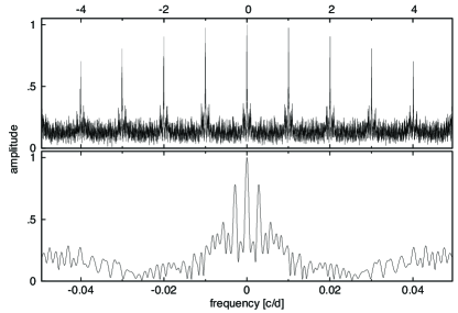
Figure 2: Spectral window of a typical well-sampled $K$-band light curve from the WFCAMCAL database, showing two different frequency ranges.

The VDFS performs an accurate and deep source extraction procedure on deep stack images, which, in the case of the WFCAMCAL database, is merged from the seven best-seeing frames to reduce any problems with blending (Cross et al. 2009). This curation step gives rise to database entities known as Sources. Positional cross-matches between these Sources and detections from different single detector frame stacks are then performed for each frame set (i.e., images with the same pointing). The prescriptions for this cross-matching procedure and its limitations are given by Hambly et al. (2008 , see their Sect. 3.4.2). Each Source of the database contains only partial information from a set of source detections positionally matched with each other, but is related to a set of pointers that track all the attributes of the corresponding detections. We note that after cross-matching, the VDFS also recalibrates the individual epochs after comparison to the deep stack to improve the light curves. The resulting source-merged catalog is stored in WSA’s relational database, which in the case of WFCAMCAL data, follows a synoptic database model designed for observations with correlated sampling (Cross et al. 2009). Since the observations of the standard star fields through different filters are always taken within a time interval that is several orders of magnitude shorter than the interval between two successive observation batches (i.e., visits of the same field, see above), they can be considered to be virtually at the same epoch. Individual source detections in different filters for each epoch (i.e., filter sequence) are therefore merged and stored in a database entity called synoptic source, and these are linked to Sources (see above). Various metadata of the time series formed by the detections associated to each Source are also provided by WSA as the attributes of the variability table, providing the best aperture for a given source, together with basic statistics on the magnitude distribution, time sampling, etc. In passing we note that this table also provides a basic assessment on the probability that a source is variable in each band, based on the comparison of the rms scatter of the time series to its expected value from a simple noise model (see Cross et al. 2009). Although these pieces of information can provide useful guidance for the user, we opted not to use these attributes as criteria in our source selection, since our aim is to perform a more profound variability search in the data.

2.2 Initial source selection

Data were retrieved in a two-step procedure via WSA’s freeform SQL query facility. We queried all Sources that were classified as a star or probable star based on the PSF statistics of the merged source, having at least ten unflagged epochs in either of the eight filter passbands.

Table 2: Number of sources, average total baseline ($\langle{T}_{\rm tot}\rangle$, in days), and average number of epochs $\langle{N}_{\rm ep}\rangle$ in each filter, in our initial database.

Filter	${N}$		$\langle{T}_{\rm tot}\rangle$	$\langle{N}_{\rm ep}\rangle$
$Z$	204,	245	1033	51
$Y$	212,	334	1061	56
$J$	212,	717	1058	58
$H$	212,	169	1074	61
$K$	201,	645	1065	60
$H_{2}$	110,	587	429	4
$Br\gamma$	130,	307	258	2
$nbj$	68,	048	120	3

Our selection resulted in an initial database of $216,\!722$ sources containing their identifiers and general attributes such as positions, basic flux, and sampling statistics. Figure 3 shows histograms of the queried light curves and the average total baseline length as a function of the number of epochs, while Tables 1 and 2 summarize some basic statistics of the queried data. The sampling of the time domain is rather heterogeneous, thus we must emphasize that the WFCAMCAL archive should not be considered as a synoptic survey database, for its completeness is highly varying from field to field; accordingly, care must be taken with any statistical interpretation based on these data. However, there are a large number of light curves with very good sampling that have $\sim 100$ data points in three to band broad-band filters, with a total baseline of up to 3 years. Since the number of data points in the narrow-band filters is generally very low, we do not use these measurements for the variability search, but they are provided (if available) for the detected variable sources in our catalog.

With the result of our first selection query at hand, we queried the complete light curves of each source by linking their entries in the Source table to the attributes of the Synoptic Source table. This procedure requires the generation of a temporary SQL table provided by the user containing the identifiers of the Sources from the first query. We note that some data, such as Julian Dates and zero-point errors, are stored in different database objects like the Multiframe table, which require the execution of further table joins. We selected magnitudes with sufficiently small error bits ($<128$), rejecting highly saturated measurements and data affected by various severe defects (e.g., bad pixels, poor flat-field region, detection close to frame boundary, etc.).

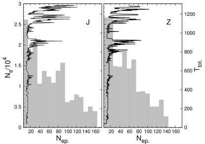
Figure 3: Histograms showing the number of sources ($N_{\rm s}$) as a function of the number of epochs ($N_{\rm ep.}$) for the queried $J$- (left) and $Z$-band (right) light curves with a bin size of 10 days. The distribution corresponding to the other broad bands are very similar. The solid curves show the average total baseline length as a function of the number of epochs for the queried light curves in the same filters with a bin width of 2 days.

3 Broad selection by variability indices

A key characteristic of the time-series data in the WFCAMCAL database is that, owing to the observation strategy, their sampling is strongly correlated in the different filters (see Sect. 2.1). The characteristic time lag between data points in different filters in an observing sequence (i.e., a standard visit of a calibration field) is not longer than a few minutes, which is orders of magnitude shorter than the typical time gap between such batches of data and also than the time scales of stellar variability at amplitudes that are typically recoverable by the present sampling and accuracy. This property of the data enables us to search for stellar variability through correlations between the temporal flux changes at different wavelengths.

In our approach to stellar variability searching, we make the following general assumptions: (i) intrinsic stellar variability is typically identifiable in a wavelength range that is wider than our broad-band filters (i.e., in more than one filter); (ii) it is sufficiently phase-locked at two close wavelengths, thus flux variations in neighboring wavebands will be correlated; and (iii) non-intrinsic variations will be typically stochastic. In point (iii) we also implicitly assume that wavelength-correlated systematics of instrumental and atmospheric origin, or due to possible data reduction anomalies, have amplitudes that are small to be enough comparable to those provided by stochastic variations. The most important deviation from this assumption for our data is due to the temporal saturation of bright objects, which can, however, be easily distinguished from stellar variability.

A commonly used approach to identifing stellar variability through correlations in flux changes is by the Welch-Stetson index ($I_{\rm WS}$; Welch & Stetson 1993; Stetson 1996). The idea behind this index is to separate stochastic variations from systematic trends by measuring the correlations in the deviations from the mean of data points that are located sufficiently close in time. It is defined as

$$I_{\rm WS}=\sqrt[]{\frac{1}{n(n-1)}}\sum_{i=1}^{n}\left(\delta b_{i}\delta v_{i}\right)\,,$$ (1)

where

$$\delta b_{i}=\frac{b_{i}-\bar{b}}{\sigma_{b,i}}\,,\leavevmode\nobreak\ \delta v_{i}=\frac{v_{i}-\bar{v}}{\sigma_{v,i}}\,,$$ (2)

with $b_{i}$, $v_{i}$, and $\sigma_{b,i},\sigma_{v,i}$ denoting magnitudes and their errors (the latter computed following the prescriptions by Stetson 1981), respectively, taken on a time scale that is much shorter than that of the intrinsic stellar variations of interest. These magnitudes and errors can represent either successive monochromatic measurements or data points taken in two different filters. We also note that $\bar{b},\bar{v}$ are weighted averages. Finally, $n$ denotes the number of epochs, by which we also refer to the number of short time slots that contain subsequently taken measurements in the case of non-simultaneously observed data with strongly correlated sampling. The $I_{\rm WS}$ index is found to be significantly more sensitive than the “traditional” $\chi^{2}$-test for single variance, which uses the magnitude-rms scatter distribution of the data as a predictor (see, e.g., Pojmanski 2002).

3.1 Extension of $I_{WS}$ to multiband datasets

According to the definition given in Eq. (1), $I_{\rm WS}$ is limited to pairwise comparisons of fluxes. When it is applied its application to panchromatic data with measurements taken in several wavebands with correlated sampling, one would need to define some conversion of the pairwise indices into a single quantity. To accomplish this, we introduce the following modification to $I_{\rm WS}$, for quantifying panchromatic flux correlations (pfc):

$$I_{\rm pfc}^{(2)}=\sqrt{\frac{(n_{2}-2)!}{n_{2}!}}\sum_{i=1}^{n}\left\{\sum_{j=1}^{m-1}\left[\sum_{k=j+1}^{m}\left(\delta u_{ij}\delta u_{ik}\right)\right]\right\}\,,$$ (3)

where $n$ is the number of epochs, $m$ is the number of wavebands, $u_{ij}$ are the flux measurements, $\delta u_{ij}$ is defined by Eq. (2) for each filter, and $n_{2}=n\cdot m!/[2!(m-2)!]$. We note that, for $m=2$, $I_{\rm pfc}^{(2)}=I_{\rm WS}$.

While Eq. (2) still measures variability through pairwise correlations of relative fluxes, we can generalize it for quasi-simultaneously measured batches of three data points (in case of $m\geq 3$) by

$$I_{\rm pfc}^{(3)}=\sqrt{\frac{(n_{3}-3)!}{n_{3}!}}\sum_{i=1}^{n}\left\{\sum_{j=1}^{m-2}\left[\sum_{k=j+1}^{m-1}\left(\sum_{l=k+1}^{m}\Lambda_{ijkl}^{(3)}\left|\delta u_{ij}\delta u_{ik}\delta u_{il}\right|\right)\right]\right\}\,,$$ (4)

where $n_{3}=n\cdot m!/[3!(m-3)!]$, and the $\Lambda$ factor is defined as

$$\Lambda_{ijkl}^{(3)}=\left\{\begin{array}[]{ll}+1&\qquad\mbox{if \,\, $\delta u_{ij}>0,\,\,\delta u_{ik}>0,\,\,\delta u_{il}>0$ };\\ +1&\qquad\mbox{if \,\, $\delta u_{ij}<0,\,\,\delta u_{ik}<0,\,\,\delta u_{il}<0$ };\\ -1&\qquad\mbox{otherwise}.\end{array}\right.$$ (5)

We note that we introduced $\Lambda^{(3)}$ to give the proper sign to the product in Eq. (4).

Finally, in the case of quasi-simultaneously measured batches of $s$ data points (for $m\geq s$), our variability index takes the following general form:

$$I_{\rm pfc}^{(s)}=\!\sqrt{\frac{(n_{s}-s)!}{n_{s}!}}\sum_{i=1}^{n}\left[\sum_{j_{1}=1}^{m-(s-1)}\!\!\!\cdots\left(\sum_{j_{s}=j_{(s-1)}+1}^{m}\!\!\!\Lambda_{ij_{1}\cdots j_{s}}^{(s)}\left|\delta u_{ij_{1}}\cdots\delta u_{ij_{s}}\right|\right)\right],$$ (6)

where $n_{s}=n\cdot m!/[s!(m-s)!]$, and the $\Lambda^{(s)}$ correction factor is

$$\Lambda_{ij_{1}\cdots j_{s}}^{(s)}=\left\{\begin{array}[]{ll}+1&\qquad\mbox{if \,\, $\delta u_{ij_{1}}>0,\,\,\cdots\,,\,\delta u_{im}>0$ };\\ +1&\qquad\mbox{if \,\, $\delta u_{ij_{1}}<0,\,\,\cdots\,,\,\delta u_{im}<0$ };\\ -1&\qquad\mbox{otherwise}.\end{array}\right.$$ (7)

Clearly, these indices set increasingly strict constraints on the presence of variability with increasing order $s$.

3.2 An alternative variability index

While the $I_{\rm pfc}^{(s)}$ index is quite robust, in the sense that it is weighted with the individual errors, it can be insensitive to true variable stars for one or several substantially outlying data points when incorrect error estimates are present. Indeed, this index may even introduce false variability candidates if these outliers are correlated in two or more bands. Although such situations might seem rare, NIR data in particular can present us with these cases quite frequently, particularly in the case of bright stars. Since the sky foreground emitted by the atmosphere is highly variable in the NIR, it causes a highly time-varying saturation limit, which can affect large parts of otherwise highly accurate time-series data for bright stars with substantial outliers having very small formal error estimates. In case of correlated sampling, these outliers will probably be correlated between different filters, leading to a spurious impact upon the $I_{\rm pfc}^{(s)}$ index.

To alleviate the effect of such anomalous outliers, we introduce an alternative variability index that is similar to $I_{\rm pfc}^{(s)}$, but does not depend on the actual value of the flux deviations from the mean. This is simply obtained by keeping only the $\Lambda$ function (Eq. 7) in the sum that appears in Eq. (6). Thus, the flux-independent (fi) version of $I_{\rm pfc}^{(2)}$ is defined as

$$2\cdot I_{\rm fi}^{(2)}-1=\frac{1}{n_{2}}\sum_{i=1}^{n}\left[\sum_{j=1}^{m-1}\left(\sum_{k=j+1}^{m}\Lambda_{ijk}^{(2)}\right)\right]\ ,$$ (8)

with $\Lambda_{ijk}^{(2)}$ defined as

$$\Lambda_{ijk}^{(2)}=\left\{\begin{array}[]{ll}+1&\qquad\mbox{if \,\, $\delta u_{ij}>0,\,\,\delta u_{ik}>0$ };\\ +1&\qquad\mbox{if \,\, $\delta u_{ij}<0,\,\,\delta u_{ik}<0$ };\\ -1&\qquad\mbox{otherwise}.\end{array}\right.$$ (9)

In this expression, the $\delta u$’s have the same meaning as before (e.g., Eq. 4).

The righthand side of Eq. (8) thus gives the difference between the number of positive and negative terms in $I_{\rm pfc}^{(s)}$, so it can only take a number of discrete values (depending on the values of $n$ and $m$). We note that, with the coefficients included on the lefthand side of Eq. (8), $I_{\rm fi}^{(2)}$ will always have absolute values between 0 and 1, analogously to a probability measure.

For higher orders $s$, $I_{\rm fi}^{(s)}$ is defined similarly to Eq. (6):

$$2\cdot I_{\rm fi}^{(s)}-1=\frac{1}{n_{s}}\sum_{i=1}^{n}\left[\sum_{j_{1}=1}^{m-(s-1)}\cdots\left(\sum_{j_{s}=j_{(s-1)+1}}^{m}\Lambda_{ij_{1}\cdots j_{s}}^{(s)}\right)\right]\,,$$ (10)

with $0\leq I_{\rm fi}^{(s)}\leq+1$, and where $\Lambda_{ij_{1}\cdots j_{s}}^{(s)}$ is defined as in Eq. (7).

Thus, the index $I_{\rm fi}^{(s)}$ represents a problem of combining signals whose function $\Lambda_{ij_{1}\cdots j_{s}}^{(s)}$ (Eq. 7) assumes the values $+1$ or $-1$, depending on the sign of the correlation. The total number of possible combinations of signals in a set of $s$ measurements, so that each group of signals is different from the other, is given by

$$A_{s}=s^{2}.$$ (11)

For the index $I_{\rm fi}^{(2)}$, for instance, we have four possible configurations, namely $(++,+-,-+,--)$. According to elementary probability theory, in the case of statistically independent events, the probability that a given event will occur is obtained by dividing the number of events of the given type by the total number of possible events. For the $I_{\rm fi}^{(s)}$ index of any order, the desired events will be those in which all signals are either positive or negative, so that, irrespective of the value of $s$, the number of events desired always equals two, and the number of possible events is given by Eq.( 11). In this way, the general expression that determines the probability value of a random event leading to a positive $I_{\rm fi}^{(s)}$ index is given by

$$P_{s}=\frac{2}{s^{2}},$$ (12)

given that there are $s^{2}$ events in total, but only two produce a positive $I_{\rm fi}^{(s)}$ value.

Figure 4: Histograms showing the number of combinations $n_{s}$ in the simulations described in the text. Since the $I_{\rm fi}^{(s)}$ index is computed in a manner similar to that used to compute the $I_{\rm pfc}^{(s)}$ index, the number of combinations used is the same for both.

3.3 Numerical tests

To establish robust criteria for selecting of variable star candidates, we evaluated the responses of the $I_{\rm pfc}^{(s)}$ and $I_{\rm fi}^{(s)}$ indices to statistical fluctuations. We generated a large number of test time-series sequences by shuffling the times (“bootstrapping”) of the WFCAMCAL data proper. By following this approach, we are able to keep part of the correlated nature of the noise intrinsic to the data, as opposed to numerical tests based on pure Gaussian noise. Figure 4 shows the histogram of the number of test time-series sequences as a function of the $n_{s}$ number of terms appearing in the variability indices (see Eqs. 6, 10) for various $s$ values. In total, $200,\!000$ realizations were performed to our tests.

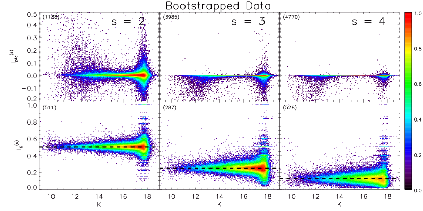
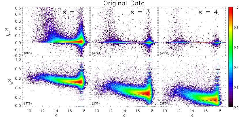
Figure 5: Variability indices versus the $K$-band magnitude, for the simulations (top two rows) and the actual data (bottom two rows), for three values of $s$, namely 2 (left), 3 (middle), and 4 (right).

Figure 5 shows the distribution of the variability indices as a function of the average apparent brightness of the sources for both the bootstrapped and the corresponding original data. The excess of high values for bright sources, which is particularly evident for $s=2$, is due to temporal saturation, which usually happens in more than one waveband at the same time. In this bright regime, as expected (Sect. 3.2), saturation affects the $I_{\rm pfc}^{(s)}$ index much more frequently than it does $I_{\rm fi}^{(s)}$. At the faint end, however, a number of effects can also be recognized. First, the quantized nature of the $I_{\rm fi}^{(s)}$ index (as opposed to the $I_{\rm pfc}^{(s)}$ index; see Sect. 3) becomes pronounced in the distribution, owing to the higher relative frequency of sources with but a few epochs (typically $n_{s}\lesssim 20$) among the faint stars. (These are often not detected if the atmospheric foreground flux is too high.) Second, there is also an excess of sources with high index values at the faint end, which is due to the much lesser amount of data for these fainter sources, which makes the variability indices more sensitive to statistical fluctuations and systematics. The general trend in the distributions of the $I_{\rm pfc}^{(s)}$ and $I_{\rm fi}^{(s)}$ are also rather different. Because it is sensitive only to the consistency in the direction of the flux changes, the $I_{\rm fi}^{(s)}$ is equally responsive to contaminating systematics of different amplitudes. This is reflected by both the slight increase in the main locus of the distribution of this index as a function of magnitude toward the bright end (see Fig. 5, lower panels) and the enhanced (false) response in the faint end, as discussed earlier. These are both caused by the increasing dominance of correlated noise over photon noise. We note that this is not shown by the bootstrapped data at the bright end, since the points of distinct pawprint batches were shuffled, and thus the correlations between them were mostly lost, while this is alleviated by the small number of points per light curve at the faint end.

Also noteworthy is that the simulated $I_{\rm fi}^{(s)}$ distributions that are shown in Figure 5 are centered on the theoretically expected values (see Sect. 3), as given by Eq. (12), namely $0.5$ in the case of $s=2$, $0.25$ in the case of $s=3$, and $0.125$ for $s=4$. Moreover, the simulation results for the $I_{\rm pfc}^{(s)}$ index show that the higher the order of the index, the lower the dispersion around $I_{\rm pfc}^{(s)}=0$; however, a pronounced level of scatter remains at both the bright and faint ends of the distribution. In addition, there is a symmetry between scatterings for the index $I_{\rm pfc}^{(2)}$ and asymmetric scattering for $I_{\rm pfc}^{(3)}$ and $I_{\rm pfc}^{(4)}$, both of which primarily scatter toward negative values, particularly at the bright end. This happens because the number of possible configurations of signs that lead to a $\Lambda=+1$ (Eq. 7) is always equal to two, whereas the number of possible configurations that lead to a $\Lambda=-1$ is instead given by $s^{2}-2$. In this way, for $s=2$, we have a symmetrical distribution of configurations of signs, whereas for $s>2$ the asymmetry in relation to negative values grows as $s^{2}-2$, as seen in the actual simulations.

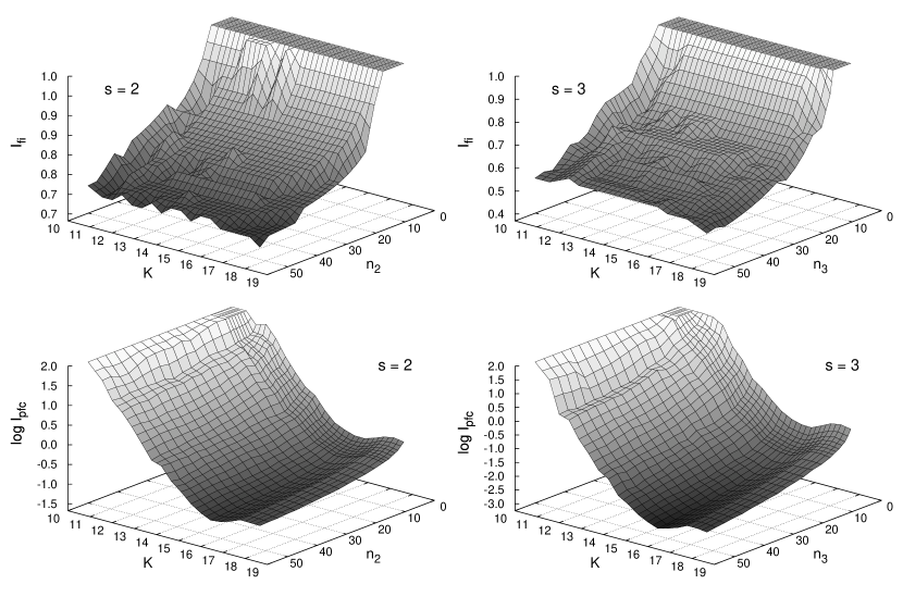
Figure 6: As in Figure 5, but for the cutoff surfaces used to select our target list, and also adding $n_{s}$ as an independent variable. These surfaces set apart, at the $0.5\%$ significance level, instances that are compatible with random noise (low values of the indices) from those that are compatible with coherent signal being present in the different passbands (high values of the indices).

We estimated the significance levels of our variability indices based on their cumulative number density distributions obtained from our bootstrapped data set. In other words, we used our bootstrap simulations to set the signals apart that are compatible with pure random noise from the signals that indicate correlated variability in the different bandpasses. We expect these estimates to be highly dependent on the number of epochs $n$ and the brightness (see above); accordingly, we obtained separate estimates for data within narrow ranges of $n$ and $K$-band average magnitude, with values in between being obtained by interpolation. Figure 6 shows the result. In this figure, we show surfaces, in $({\rm index},n_{s},K)$ space that set random noise apart from correlated signals at the $0.5\%$ significance level, according to our two variability indices, namely $I_{\rm pfc}^{(s)}$ (top row) and $I_{\rm fi}^{(s)}$ (bottom row). As can be seen from Figure 6, the corresponding cutoff values of the $I_{\rm fi}^{(s)}$ variability index show a relatively weak dependence on the magnitude and a strong dependence on $n_{s}$, whereas the $I_{\rm pfc}^{(s)}$ index depends strongly on both of these quantities. This is mainly attributed to the fact that the mean values of the formal errors (estimated from photon noise only), to which $I_{\rm pfc}^{(s)}$ is very sensitive, increasingly underestimate the global scatter of the light curves toward lower magnitudes in this dataset.

3.4 Initial selection of variable star candidates

We next computed the variability indices introduced in Sect. 3 for all sources in our initial database. As many as $99.3\%$ of these sources had quasi-simultaneous observations in at least two filters, while $91.3\%$ and $81.3\%$ of them were observed in at least three and four filters, respectively. For each variability index, we selected all sources above its empirical, sampling, and magnitude-dependent 0.5% significance level described in Sect. 3.3. We considered a source as a candidate variable star if either value of its variability indices was significant. This procedure resulted in our initial catalog of 6651 candidate variable stars.

4 Frequency analysis

There are many methods available for computing periods in unevenly spaced time-series data, based mainly on Fourier analysis, information theory, and statistical techniques, among others (see, e.g., Templeton 2004 , for a review). Some of these methods are based on the fact that the phase diagram of the light curve (also known as simply “phased light curve”) is smoothest when it is visualized using its real period. They transform the set of data by folding within the phase interval $0\leq\varphi(i)<1$, which is defined by the following expression:

$$\varphi(i)=\frac{t(i)-t_{0}}{P}-{\rm INT}\left[\frac{t(i)-t_{0}}{P}\right],$$ (13)

where $t$ is the time, $t_{0}$ is the time origin, $P$ is a test period, and ${\rm INT}$ denotes the integer function. Because of the presence of observational gaps, it often happens that computed phases can have the same numerical values for several different test periods. Many periods are spurious because they correspond to gaps that may be present in the data (e.g., daytime, seasons, etc.; Lafler & Kinman 1965). If $P$ is the true period and $P_{\rm gaps}$ the period of gaps (Damerdji et al. 2007), spurious periods are given by

$$P_{\rm spur}^{-1}=P^{-1}\pm k\,P_{\rm gaps}^{-1},$$ (14)

where $k\in\mathbb{N}$. In some cases, a spurious period could be ranked as the best period.

We searched for periodic variable stars in our initial catalog (see Sect. 3.4) by applying various frequency analysis methods in combination. To search for the best period (or, equivalently, frequency), many methods require that a search range (given by limiting frequencies $f_{0}$ and $f_{N}$ at the low- and high-frequency ends, respectively) and resolution $\Delta f$ be specified first. Since we are dealing with data sets with various different time spans, we adapted the $f_{0}$ low-frequency limits to each light curve by $f_{0}=0.5/T_{\rm tot}$, where $T_{\rm tot}$ is the total baseline of the observations, and we scaled the $\Delta f$ frequency resolution bas $\Delta f=0.1/T_{\rm tot}$. The method described by Eyer & Bartholdi (1999) was used to determine the high-frequency limit $f_{N}$.

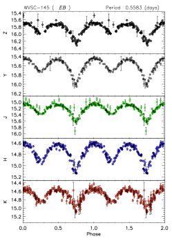
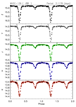
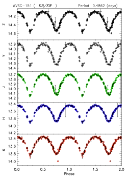
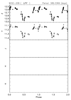
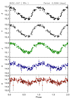
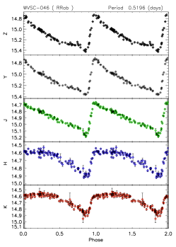
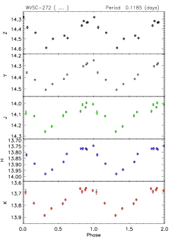
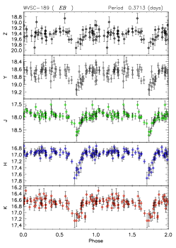
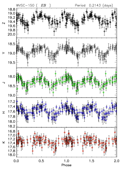
Figure 7: Phase-folded light curves of selected objects from our catalog of periodic variables (C1), showing data in all five broadband filters of WFCAM. ID’s, types, and periods for each object are shown in the headers. The object WVSC-208 was only detected in the $Z$ and $Y$ bands.

Initially, we applied the string-length minimization (SLM; Lafler & Kinman 1965; Stetson 1996) method on the light curves in our initial catalog of candidate variable stars. In this method, the period is found by minimizing the sum of the lengths of the segments joining adjacent points in the phase diagrams (called the “string lengths”) using a series of trial periods, i.e.:

$$\Phi=\frac{\sum_{i=1}^{N-1}w_{i,i+1}\left|m_{i+1}+m_{i}\right|}{\sum_{i=1}^{N-1}w_{i,i+1}},$$ (15)

where

$$w_{i,i+1}=\frac{1}{\left(\sigma_{i+1}^{2}+\sigma_{i}^{2}\right)\left(\varphi_{i+1}-\varphi_{i}+\epsilon\right)},$$ (16)

and $\varphi_{i}$, $m_{i}$, and $\sigma_{i}$ are phases, magnitudes, and corresponding magnitude uncertainties, respectively, sorted in order of increasing phase according to the trial period. The variable $\epsilon$ is a term that is added to reduce the weight of very closely spaced data in phase space, which otherwise could have a weight approaching infinity (Stetson 1996). In our work, we assumed $\epsilon=1/N$, again following Stetson (1996).

To increase the probability that among the higher peaks of the periodogram derived on the basis of the SLM method the best period is included, we took the following additional steps:

• The SLM periodogram was independently computed for each broadband filter ($Y$, $Z$, $J$, $H$, and $K$), based on which all periods that presented a power greater than the $3\sigma$ level every band were selected;

• The SLM periodogram was also computed for the chromatic light curve, comprised of the sum of all broadband filters, and again all periods above the $3\sigma$ level were selected;

• The results of the previous two steps were then combined, yielding the best periods (i.e., the ones with the highest amplitude peaks) from both types of analysis.

These steps are very important, because the same source can have photometry of high quality in some filters, but not others.

In the second step of the period search, we applied three additional frequency analysis methods, to select the ten best among the periods selected by the SLM method. For this step, we used the “classical” Lomb-Scargle (LS) periodogram (Lomb 1976; Scargle 1982), the generalized Lomb-Scargle (GLS) periodogram (Zechmeister & Külrster 2009), and the phase dispersion minimization (PDM; Stellingwerf 1978) methods. We included both LS and GLS because the latter gives unbiased estimates of the standard deviation of the measurements only when the photometric errors are good, easily leading to spurious results otherwise. The PDM method was included due to its high sensitivity to highly non-sinusoidal variations with alternating peaks, as in the case of the light curves of eclipsing binary systems.

We proceeded with our analysis as follows:

• For all light curves that were preselected by the SLM method, we independently computed the periodogram using each of these methods and for each filter separately;

• After inverting the spectra from the PDM and SLM methods, the periodograms for each filter were then normalized by the maximum power;

• A single, normalized power spectrum was then obtained for each method by averaging over all filters the results obtained in the previous step for each filter independently;

• Finally, we obtained a ranked list of the best periods for each method.

The best periods should in principle be those that ranked highest in all four methods. However, not all methods rank periods in the same way. Therefore, to choose of periods in a more objective fashion, we computed a “super rank” index as the sum of the ranks provided by each of these five methods. We then selected the ten best periods as those ten most highly ranked, according to this new index.

Finally, in order to select the very best period, we use the $\chi^{2}$ test, in which Fourier coefficients $(a_{0},a_{i},b_{i})$ are derived that fit the data according to the following expression:

$$f(i)=a_{0}+\sum_{i=1}^{n}\left\{a_{i}\sin\left[2k\pi\varphi(i)\right]+b_{i}\cos\left[2k\pi\varphi(i)\right]\right\},$$ (17)

where $k=1/P$. We used the Levenberg-Marquardt (Levenberg 1944; Marquardt 1963) method to find the solutions and employed the statistical F-test to evaluate the results. We limited the amplitude of the fit to the observed magnitude range $(m_{\rm max}-m_{\rm min})$ and kept the number of harmonics to $n\leq 20$. The period that produced the lowest reduced $\chi^{2}$ value was selected as the true main period. Finally, we visually inspected of the phase diagrams, which narrowed down our selection to our final catalog containing 275 periodic variable stars, as described in more detail in the next section.

5 Results and discussions

5.1 Catalog of periodic variable stars (C1)

Proceeding as described in the previous section, we have thus obtained our final sample of 275 clearly periodic variable stars (C1). Their coordinates, periods, mean magnitudes, and the number of epochs in each filter are listed in Table 5. We also provide preliminary classifications for most of the newly discovered variables. The variability types of these sources were assigned by visual inspection of their phase diagrams, and are also listed in Table 5, using the nomenclature of the General Catalog of Variable Stars (GCVS, Samus 1977). Phase-folded light curves for some of these objects are shown in Figure 7.

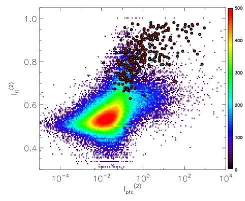
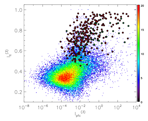
Figure 8: Distribution of $I_{\rm fi}$ versus $I_{\rm pfc}$ variability indices, for orders 2 (left) and 3 (right). The C1 and C2 sources are indicated by red and green circles, respectively.

5.2 Catalog of aperiodic variable stars (C2)

We also searched for those stars that, in spite of showing reasonably coherent light curves, do not show a clear main periodicity in the WFCAMCAL data, either because their variations are intrinsically aperiodic or because they have such long periods that these data were insufficient for deriving them. To identify such sources, we relied only on the variability indices, requiring that these have highly significant values, indicating the presence of correlated variations in the different WFCAM bandpasses. First, we selected sources by using a strong cutoff at the sampling- and magnitude-dependent 0.1% significance level, equivalently to the procedure described in Sect. 3.4. Table 3 shows the number of selected sources based on each of the cutoff surfaces shown in Figure 5, before and after visual inspection. The number of sources selected by the $I_{\rm fi}^{(s)}$ index is less than a third of the sources selected using the $I_{\rm pfc}^{(s)}$ index, and at the same time, it includes 80% of all sources in C1 (Sect. 5.1). This high efficiency at a relatively low false alarm rate favored the application of the $I_{\rm fi}^{(s)}$ index alone for selecting aperiodic variable candidates, which was followed by a visual inspection in order to reject likely false candidates.

Our procedure has led to an additional 44 sources, comprising our catalog of semi-regular or aperiodic variable stars and stars with uncertain periods (C2), shown in Table LABEL:tab-cat02. The selected variable star candidates, including both periodic (C1) and non-periodic (C2) sources, are shown in the [$I_{\rm fi}^{(s)}$, $I_{\rm pfc}^{(s)}$] plane (for $s=2$ and 3) in Figure 8. This figure clearly shows that the $I_{\rm fi}^{(s)}$ index is significantly more powerful, as far as distinguishing the variability in the WFCAM data is concerned, compared with the $I_{\rm pfc}^{(s)}$ index, since there is much less overlap between variable and non-variable sources in the former than the latter. As a word of caution, we note that the C2 catalog could still contain spurious sources, mainly due to sources that show correlated seasonal variations and/or correlated noise variations. Follow-up studies of these sources is thus strongly recommended, before conclusively establishing their variability status.

Table 3: Number of variable star candidates selected by the different variability indices at different significance levels before and after (in parentheses) visual inspection.

Sign. level	$I_{\rm pfc}^{(2)}$	$I_{\rm pfc}^{(3)}$	$I_{\rm fi}^{(2)}$	$I_{\rm fi}^{(3)}$
0.5%	4598(219)	3574(192)	1292(242)	1045(242)
0.1%	1676(145)	1337(141)	466(186)	398(190)

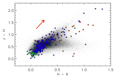
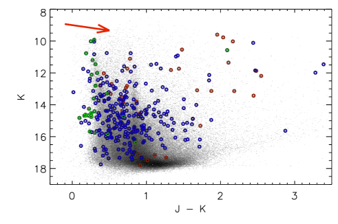
Figure 9: Color-color (on left panel) and color-magnitude (right panel) diagrams of the analyzed sample. New objects in C1 (in blue) and C2 (in red) and previously known objects (in green) are shown with colored points. Red arrows indicate the reddening vectors.

5.3 Cross-identifications

As the final step in our analysis, we performed a systematic cross-check of the sample of 319 sources in C1 and C2 catalogs to identify previously known sources and complement our catalog with data already in the literature. Among the cross-checked catalogs, one finds the SIMBAD database, the latest version of the General Catalog of Variable Stars (Samus et al. 2012), the AAVSO International Variable Star Index (VSX v1.1, now including 284,893 variable stars; Watson et al. 2014), the New Catalog of Suspected Variable Stars (Kazarovets et al. 1998), and the Northern Sky Variability Survey (NSVS; Hoffman et al. 2009) catalog, among many other databases incorporated in the International Virtual Observatory Alliance (IVOA), using the Astrogrid facility.

A delicate issue that we face when performing these extensive cross-checks between surveys with such diverse technical properties is their different astrometric accuracy. In this sense, we assumed a positional accuracy of $2\arcsec$ in the sky coordinates for WFCAM, and then used optimized search radii according to the specific nature of each cross-matched database.

Taking the distribution of our sources across the sky into account, along with the specific nature of the observations that comprise the WFCAMCAL catalog, which were aimed at observing standard star fields and hence tended to avoid very crowded regions, it did not come as a surprise that the cross-checking with variability surveys of the southern sky and Galactic central regions, such as OGLE, MACHO, and ASAS, did not result in any positive match. We extended the search further to other astronomical catalogs of non stellar and/or extragalactic objects (e.g., planetary nebulae, quasars, optical counterparts of GRBs, just to mention a few) and in different spectral bands (from radio to X-rays), but again finding no superpositions with our WFCAM sources.

At the end of this search, we found a total of 44 stars that were already known from previous studies. Among them, 37 sources are included in the VSX catalog, three of which are also GCVS objects (i.e., AM Tau, EH Lyn, UV Vir, which are an Algol-type eclipsing binary, a contact binary, and an ab-type RR Lyrae, respectively). The GCVS also lists five other eclipsing binaries and another RRab Lyrae (HM Vir).

The outer part of the globular cluster M3 (NGC 5272) is also partly covered by the WFCAMCAL pointings. Indeed, among our preselected variable candidates, we were able to recover 11 stars that had already been identified as RR Lyrae stars by Cacciari et al. (2005), Jurcsik et al. (2012), and Watson et al. (2014). Cross-identifications and literature variability types of the previously known sources are given for C1 and C2 in Tables LABEL:tab-cat01 and LABEL:tab-cat02, respectively.

5.4 Detection efficiency

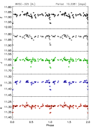
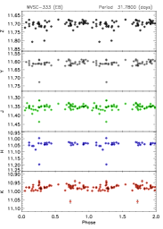
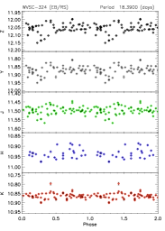
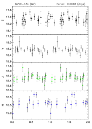
Figure 10: Example light curves of 4 previously known variable stars that were not detected in our analysis. ID’s, variability types, and periods for each star are shown in the headers.

To estimate the variable star detection efficiency of our method, we determined whether any variable stars in the WFCAM calibration fields that are known from other catalogs were not detected by us. Similar to the procedure described in Sect. 5.3, we performed positional cross-matches of our initial database of $216,\!722$ light curves with all existing survey catalogs of variable stars incorporated in the IVOA. We found a total of 15 known variables (all of them periodic) that were missed by our search. Thirteen of them were excluded in the first broad selection phase (see Sect. 3) owing to the low values of their variability indices. The properties of these stars are listed in Table LABEL:tab-cat03, and their WFCAM photometry is added to our catalog of periodic variable stars (C1), including a flag that refers to their non-detection as variables by our analysis.

Figure 10 shows four typical examples among the non-detected variables. The non-detection of these sources is either due to the insufficient phase coverage of their magnitude variations by WFCAM data (primarily in the cases of long-periodic eclipsing binaries with very low fractional transit lengths, see Fig. 10, upper panels) or due to saturation (Fig. 10, lower left panel) or to a very low signal-to-noise ratio.

Since the heterogeneity and small number of objects known from other variable star catalogs overlap with the WFCAMCAL fields make them insufficient for a quantitative assessment of our detection efficiency, we performed further tests using synthetic data. To do this we first built a database of noise-free LCs as being harmonic fits (see Eq. 17) of actual C1 data, in each filter. Next, we generated $10^{5}$ synthetic light curves, following the distributions of periods, amplitudes, and sampling of the final C1 catalog. Then, these synthetic light curves were added to segments of the real light curves of non-variable stars from the WFCAMCAL database. Finally, we applied the same procedures of variability search and period analysis that we discussed in Sections 3 and 4 on the simulated data.

The result of our test is summarized by Figure 11, which shows the detection efficiency $E_{det.}=N_{det.}/N_{all}$ as a function of $K$ magnitude using bins of 0.25 mag, where $N_{det.}$ is the number of detected variables, and $N_{all}$ is the number of all variables, respectively. Based on this test, we estimate an average detection efficiency of $93\%$ over the complete magnitude range of the WFCAM database. Detection rates lower than $90\%$ are only present in the two extremes of the magnitude range, dominated by saturation in the bright end and low signal-to-noise ratio in the faint end. We note that the lower overall detection efficiency suggested by the catalog cross-matches is due to the biased magnitude distribution of the cross-matched sources toward the bright end of the WFCAM magnitude range.

Figure 11: Detection efficiency $E_{det.}$ vs $K$ mean magnitude for $10^{5}$ synthetic variables.

5.5 Photometric properties of the variables

Figure 9 shows the variable and non-variable sources on the $(H-K)-(J-H)$ color-color and the $K-(J-K)$ color-magnitude planes. The variable sources cover the entire range of stellar parameter space in these planes. It is also clear from this figure that the area covered by the WFCAM Calibration fields have significant differential reddening, and a great fraction of the variables are reddened sources. This, together with the large aperture of the UKIRT telescope, explains the relatively low number of cross-identifications with previously known objects (Sect. 5.3): the WFCAMCAL database covers a range of faint NIR magnitudes where most of the optical variability surveys cannot penetrate, while most of the known variables in those catalogs are too bright for WFCAM.

We found 32 highly reddened ($Z-K>3$) variable sources, 17 of which are periodic. We found that the positions of these red sources are strongly clustered around the positions $\alpha=18^{\rm h}29.5^{\rm m},\leavevmode\nobreak\ \delta=+1^{\circ}36^{\prime}$ (25 sources), and $\alpha=7^{\rm h}0^{\rm m},\leavevmode\nobreak\ \delta=-4^{\circ}51^{\prime}$ (8 sources). They are surrounded by a number of dark nebulae previously cataloged by Dobashi (2011) and Dutra & Bica (2002), respectively, suggesting that these sources might be embedded young stellar objects (see Tables LABEL:tab-cat01, LABEL:tab-cat02).

6 Conclusions

In this paper, we have established the WFCAM Variable Star Catalog, based on a detailed analysis of the WFCAMCAL NIR database. Our catalog contains 319 variable point sources, among which are 275 that are clearly periodic, and it includes 44 previously known objects. All catalog entries including multiband light curve data are available online via the WFCAM Science Archive (WSA) . Our approach to variability analysis included introducing a new, flux-independent variability index that is highly insensitive to the presence of outliers in the time-series data. A cross-matching procedure with previous variable star catalogs was also carried out, and the few sources with previous identification in the literature are noted. These catalogs represent one of the first such resource in the NIR, and thus an important first step toward the interpretation of future, more extensive NIR variability datasets, such as will be provided by the Vista Variables in the Vía Láctea (VVV) Survey in particular (Catelan et al. 2013). A more detailed analysis of the different classes of variable stars detected in our catalog will be presented in a forthcoming paper.

landscape

Table 4: Periodic objects in the WFCAM Variable Star Catalog (C1)

ID [WSA]	ID [WVSC]	ID	RA [deg.]	DEC [deg.]	type	P [d]	$\langle Z\rangle$	$\langle Y\rangle$	$\langle J\rangle$	$\langle H\rangle$	$\langle K\rangle$	$N_{Z}$	$N_{Y}$	$N_{J}$	$N_{H}$	$N_{K}$
858993461311	WVSC-001	UNC	146.283535	59.539435	UNC	0.158027	16.884	16.623	16.192	15.723	15.550	10	10	18	16	16
858993464444	WVSC-002	UNC	145.560146	59.046595	RR	0.49192	16.936	16.912	16.697	16.516	16.579	10	9	19	16	17
858993475542	WVSC-003	CSS_J033147.8+374651	52.949484	37.780864	EW	0.247579	15.796	15.522	15.013	14.385	14.188	59	79	91	84	93
858993476434	WVSC-004	CSS_J033109.1+375343	52.788116	37.895692	EW	0.286644	16.611	16.350	15.911	15.345	15.163	57	76	87	79	84
858993477934	WVSC-005	UNC	53.345266	37.87284	UNC	0.127022	18.874	18.470	17.814	17.199	16.974	54	72	81	73	77
858993478382	WVSC-006	UNC	53.424094	37.81507	UNC	2.4277	16.261	15.907	15.326	14.636	14.346	60	78	87	82	90
858993479072	WVSC-007	UNC	53.53775	37.853985	EB?	1.7298	18.447	18.008	17.327	16.652	16.370	55	74	83	75	81
858993484033	WVSC-008	UNC	9.491549	37.781801	MP?	10.205	16.733	16.561	16.078	15.633	15.412	99	102	115	114	117
858993534207	WVSC-009	CSS_J033354.2+372322	53.476152	37.389687	EW	0.262090	15.289	14.744	14.181	13.406	13.109	58	79	92	85	94
858993535184	WVSC-010	CSS_J033319.1+371524	53.329849	37.256611	EW	0.299889	15.839	15.608	15.242	14.803	14.572	57	78	91	84	93
858993539168	WVSC-011	UNC	52.912129	37.39636	EB	0.295638	19.236	18.798	18.249	17.572	17.440	45	65	77	70	72
858993544979	WVSC-012	UNC	9.541155	37.206287	LP?	12.578	15.318	15.096	14.708	14.182	14.047	99	102	115	115	118
858993546108	WVSC-013	UNC	9.151256	37.293481	EB/EW	0.400364	11.733	11.672	11.467	11.251	11.192	90	94	115	110	119
858993549466	WVSC-014	NSVS 7772290	224.808071	37.042755	RRab	0.63019	14.143	14.092	13.899	13.697	13.609	77	5	107	101	114
858993598145	WVSC-015	LINEAR 19154958	250.150045	36.819243	EA	0.506418	13.647	13.490	13.109	12.633	12.509	68	73	84	76	83
858993603097	WVSC-016	UNC	250.399529	36.464598	WV	1.22670	15.774	15.733	15.429	14.794	14.726	4	3	17	15	38
858993615087	WVSC-017	LINEAR 18385620	+246.5010500	+34.8893750	DSCT	0.056949	15.620	15.637	15.456	15.410	15.401	55	62	65	63	65
858993625957	WVSC-018	V1183 Her	247.123266	34.530253	EW?	0.309504	11.623	11.500	11.216	10.856	10.751	53	50	61	21	58
858993630922	WVSC-019	V* EH Lyn	135.667523	34.329637	EW	0.326744	13.383	13.347	13.117	12.903	12.804	81	84	113	96	113
858993632337	WVSC-020	UNC	316.035368	30.851989	WV?	0.153950	17.724	17.629	17.284	16.945	16.853	100	105	104	98	86
858993633031	WVSC-021	UNC	316.047441	30.885523	BD?	6.398	15.237	15.043	14.635	14.111	13.959	102	106	126	117	126
858993634274	WVSC-022	UNC	316.109244	30.942416	EB	0.68287	17.393	17.403	17.200	16.917	16.893	100	104	116	106	97
858993635978	WVSC-023	UNC	316.00418	31.013522	EB	0.254721	18.550	18.430	17.965	17.513	17.324	90	96	92	80	69
858993636075	WVSC-024	UNC	315.939706	31.017482	EB?	0.110912	18.124	17.894	17.345	16.737	16.564	99	102	114	112	116
858993637017	WVSC-025	UNC	315.868607	31.055426	EB	0.76859	14.497	14.426	14.212	13.974	13.900	103	106	126	117	115
858993640688	WVSC-026	UNC	316.392944	30.965097	EB	0.283741	17.438	16.911	16.248	15.628	15.282	100	104	125	117	126
858993642335	WVSC-027	UNC	316.478532	31.054465	EB?	0.382816	17.272	17.105	16.713	16.205	16.002	100	103	124	117	126
858993643289	WVSC-028	UNC	316.529965	30.835178	EB/EW	0.372206	17.789	17.601	17.264	16.924	16.804	8	7	53	64	110
858993643597	WVSC-029	UNC	316.546651	30.920522	EB?	1.13248	14.072	13.924	13.562	13.147	12.998	80	64	107	104	126
858993644865	WVSC-030	UNC	316.623841	31.005224	BD?	2.39238	14.459	14.363	13.993	13.462	13.324	17	15	36	30	35
858993651058	WVSC-031	UNC	316.552954	30.573486	EB	0.272796	15.902	15.745	15.460	14.940	14.828	99	104	125	116	127
858993651463	WVSC-032	UNC	316.509624	30.55661	EB	0.9995	12.831	12.768	12.592	12.349	12.348	102	102	123	103	100
858993651583	WVSC-033	UNC	316.440931	30.550424	EB	0.74530	17.161	16.964	16.566	16.007	15.850	101	104	122	115	127
858993653343	WVSC-034	UNC	316.398603	30.473811	EB/EW	0.289408	16.942	16.736	16.280	15.879	15.767	102	105	124	117	127
858993654890	WVSC-035	UNC	316.495184	30.398145	EB/EW	0.305103	15.326	15.189	14.857	14.502	14.384	101	104	126	117	127
858993657176	WVSC-036	UNC	316.117947	30.418146	EB/EW	0.205387	15.223	15.101	14.837	14.484	14.376	18	15	85	90	120
858993657640	WVSC-037	UNC	316.096904	30.449857	RR	0.64670	16.613	16.483	16.203	15.815	15.803	101	104	124	117	127
858993659737	WVSC-038	UNC	316.006495	30.546451	EB	0.41158	17.525	17.257	16.864	16.354	16.272	100	105	117	112	117
858993661749	WVSC-039	UNC	315.914246	30.446447	EB?	0.56763	17.310	17.072	16.499	15.937	15.680	101	102	124	117	127
858993661905	WVSC-040	1SWASP J210337.93+302659.2	315.908006	30.449801	EA	1.9353	10.626	10.549	10.330	10.144	10.034	3	4	60	21	83
858993670937	WVSC-041	UNC	112.290496	30.304305	EB	1.3317	15.177	15.124	14.869	14.585	14.516	64	72	86	79	88
858993671407	WVSC-042	UNC	112.186982	30.380001	EB	0.384516	17.432	17.093	16.481	15.926	15.603	64	72	85	79	87
858993673691	WVSC-043	UNC	112.610889	30.314442	MP?	1.3451	14.399	14.145	13.658	13.009	12.815	67	73	86	78	85
858993758351	WVSC-044	NGC 5272 338	205.502796	28.477732	RRc	0.329593	15.142	15.130	14.922	14.849	14.825	17	11	22	20	11
858993759574	WVSC-045	NGC 5272 279	205.483503	28.413613	RRab	0.558013	15.015	15.039	14.830	14.603	14.579	63	82	101	100	126
858993759604	WVSC-046	NGC 5272 278	205.48296	28.468236	RRab	0.529819	15.106	15.080	14.801	14.587	14.624	69	73	79	78	102
858993759856	WVSC-047	NGC 5272 264	205.478231	28.464431	RRab	0.519611	15.121	15.072	14.892	14.676	14.674	74	87	101	100	126
858993760097	WVSC-048	NGC 5272 253	205.473144	28.423797	RRc	0.326640	15.175	15.151	15.011	14.847	14.754	84	91	101	100	126
858993760236	WVSC-049	NGC 5272 249	205.470686	28.411781	RRab	0.587083	15.012	14.902	14.781	14.550	14.525	83	91	101	100	126
858993760605	WVSC-050	NGC 5272 234	205.462206	28.409174	RRab	0.551543	15.116	15.051	14.857	14.641	14.607	80	90	101	100	126
858993760902	WVSC-051	NGC 5272 223	205.454101	28.442241	RRab	0.640116	14.906	14.869	14.716	14.472	14.412	51	48	57	54	117
858993761631	WVSC-052	UNC	205.429057	28.40102	EB	0.445936	18.350	18.381	18.123	17.948	17.730	83	89	86	73	28
858993761656	WVSC-053	NGC 5272 190	205.428466	28.404882	RRab	0.773532	14.820	14.775	14.480	14.227	14.254	62	66	101	100	126
858993762099	WVSC-054	NGC 5272 181	205.40833	28.409307	RRab	0.501263	15.149	15.116	14.847	14.715	14.683	84	90	102	100	125
858993762390	WVSC-055	NGC 5272 170	205.391872	28.506926	RRab	0.514803	15.045	14.958	14.842	14.668	14.666	85	91	101	100	126
858993765388	WVSC-056	UNC	65.825989	26.68764	EB?	6.479	-9.999	14.047	12.553	11.022	10.113	1	47	67	28	15
858993765544	WVSC-057	UNC	65.806081	26.746206	RCB/EB?	10.019	-9.999	15.097	13.977	12.726	12.130	1	47	67	64	67
858993765662	WVSC-058	UNC	65.978024	26.770083	EB?	0.121704	-9.999	18.815	17.903	16.639	16.182	1	41	63	61	65
858993770774	WVSC-059	UNC	66.413625	26.119562	EB	0.419303	-9.999	17.013	16.540	15.915	15.687	0	45	69	64	70
858993772561	WVSC-060	UNC	65.962096	26.239973	MP?	2.5556	-9.999	13.305	13.053	12.758	12.635	0	52	70	64	69
858993772880	WVSC-061	UNC	65.904342	26.119991	EB?	0.328507	-9.999	16.168	15.632	14.888	14.738	0	52	70	65	68
858993835928	WVSC-062	CSS_J042001.7+171645	65.007363	17.27938	WV	33.29	15.292	14.957	14.524	14.119	13.934	51	82	95	92	95
858993837402	WVSC-063	UNC	65.392169	17.113222	EB	0.626686	13.545	13.409	13.164	12.907	12.784	34	78	93	91	93
858993844067	WVSC-064	UNC	87.672286	16.231257	EB?	0.625369	14.951	14.751	14.328	13.826	13.697	89	119	136	131	136
858993844518	WVSC-065	UNC	87.75716	16.254779	RR?	0.161579	13.532	13.392	13.053	12.686	12.582	90	121	135	131	135
858993845424	WVSC-066	UNC	87.667203	16.307342	EB	1.6095	14.611	14.486	14.223	13.916	13.791	90	121	136	132	136
858993846025	WVSC-067	UNC	87.744499	16.337318	RR/EW?	0.387056	15.939	15.804	15.460	15.076	14.986	89	120	136	131	136
858993846345	WVSC-068	UNC	87.571443	16.356207	EB	0.382237	16.571	16.177	15.583	14.888	14.588	88	121	135	131	135
858993847117	WVSC-069	UNC	87.68201	16.397512	EB?	0.117309	17.294	17.132	16.665	16.206	16.065	89	121	136	131	136
858993847751	WVSC-070	UNC	87.740914	16.431696	UNC	0.257344	14.136	13.930	13.716	13.432	13.341	8	13	74	101	123
858993851860	WVSC-071	UNC	88.08328	16.416697	EB?	0.153861	16.394	16.197	15.803	15.323	15.198	101	121	137	131	135
858993852012	WVSC-072	V* AM Tau	88.089084	16.283537	EA/SD	2.04387	10.531	10.461	10.224	10.054	9.907	4	11	44	6	20
858993852658	WVSC-073	UNC	88.126444	16.367541	UNC	0.12815	17.237	16.960	16.617	16.184	15.983	98	121	138	132	135
858993854681	WVSC-074	UNC	88.215008	16.359551	EB/EW	0.187452	14.292	14.094	13.855	13.532	13.467	102	120	136	132	135
858993855085	WVSC-075	UNC	88.231993	16.247183	EB	0.148999	16.550	16.443	16.090	15.746	15.601	97	117	136	131	135
858993855285	WVSC-076	UNC	88.23866	16.390559	EB?	0.118653	17.793	17.449	16.926	16.195	16.101	85	117	134	130	131
858993860218	WVSC-077	UNC	88.195444	15.950907	RR?	0.120533	17.233	17.012	16.481	15.817	15.535	105	117	134	126	131
858993860697	WVSC-078	UNC	88.134228	15.923956	EB	0.321011	17.076	16.977	16.602	16.255	16.069	108	120	137	129	135
858993860784	WVSC-079	UNC	88.123632	15.918918	EB	0.85505	16.376	16.240	15.954	15.673	15.586	111	121	137	129	135
858993861924	WVSC-080	UNC	88.136087	15.854916	EB	0.302547	17.166	16.986	16.575	16.287	16.103	110	120	137	127	135
858993863119	WVSC-081	UNC	88.115593	15.78848	EB?	0.143696	17.793	17.591	17.158	16.589	16.452	93	119	133	125	133
858993867117	WVSC-082	UNC	87.726811	15.845016	RR/EW	0.31857	16.000	15.813	15.475	15.091	14.909	112	120	136	132	136
858993867644	WVSC-083	UNC	87.696811	15.916248	UNC	0.146051	17.605	17.478	17.054	16.730	16.636	103	120	135	131	133
858993875271	WVSC-084	V* HS Cnc	132.770127	11.765788	EW	0.359664	12.604	12.456	12.333	11.977	11.998	59	57	67	60	70
858993876013	WVSC-085	V* ES Cnc	132.836634	11.890588	EA/RS	0.532046	10.487	10.478	10.272	10.086	10.021	6	5	23	8	25
858993876386	WVSC-086	V* EV Cnc	132.867279	11.824295	EW/KW	0.441443	12.021	11.968	11.765	11.536	11.453	55	55	67	49	70
858993876850	WVSC-087	V* AH Cnc	132.907685	11.849185	EW/KW	0.360461	12.651	12.575	12.370	12.147	12.109	56	58	67	61	70
858993882292	WVSC-088	Cl* M67 XZD 3	132.339004	11.324518	EW	0.87684	14.187	14.068	13.770	13.385	13.302	58	56	67	61	69
858993882503	WVSC-089	CSS_J084911.7+112816	132.299364	11.471132	EA	0.284996	13.374	12.967	12.442	11.861	11.602	58	56	67	61	69
858993887204	WVSC-090	CSS_J231223.8+111339	348.099701	11.2279	RRd	0.290866	15.412	15.366	15.247	14.958	14.905	111	112	127	121	128
858993887341	WVSC-091	UNC	348.132532	11.22061	EB?	1.7476	13.079	13.023	12.787	12.501	12.439	110	111	127	121	128
858993887483	WVSC-092	UNC	348.174214	11.136043	EB?	2.7558	14.020	13.722	13.330	12.731	12.556	109	110	127	123	128
858993939587	WVSC-093	UNC	312.839437	6.558035	EB	1.3866	12.041	12.026	11.901	11.765	11.749	81	70	121	133	142
858993943395	WVSC-094	UNC	313.096957	6.636626	SR?	10.468	14.995	14.788	14.365	13.803	13.673	142	142	160	157	167
858993944520	WVSC-095	UNC	313.162131	6.580543	EB	0.401346	11.425	11.374	11.126	10.903	10.830	73	75	118	54	122
858993945235	WVSC-096	UNC	313.208491	6.758572	EB?	4.5955	13.797	13.593	13.270	12.879	12.770	13	8	56	72	136
858993946452	WVSC-097	UNC	313.299863	6.745278	RR/EW?	0.135439	17.929	17.872	17.606	17.231	17.192	138	140	137	143	111
858993949722	WVSC-098	UNC	313.145596	6.315533	EB	2.3951	14.369	14.049	13.546	12.874	12.680	142	142	162	156	167
858993950831	WVSC-099	CSS_J205225.3+061500	313.105533	6.25005	RRab	0.539025	16.272	16.226	15.984	15.735	15.624	141	142	161	155	164
858993951816	WVSC-100	CSS_J205306.4+061054	313.276707	6.18187	EA	0.84644	15.404	15.339	15.117	14.858	14.789	136	136	157	125	148
858993952160	WVSC-101	UNC	313.26843	6.15111	RR/EB?	0.138725	14.628	14.536	14.136	13.745	13.650	141	141	162	156	168
858993966899	WVSC-102	UNC	127.903487	5.90891	UNC	4.2395	17.785	17.529	17.167	16.597	16.394	70	86	90	87	91
858993968747	WVSC-103	UNC	246.734916	5.867772	EB	0.169992	15.821	15.533	15.052	14.449	14.216	58	71	77	72	78
858994013738	WVSC-104	CSS_J083048.8+053543	127.703875	5.595349	EW	0.271745	15.760	15.622	15.247	14.760	14.633	78	83	92	86	94
858994015625	WVSC-105	CSS_J082950.2+052907	127.459127	5.485724	EA	0.77666	15.638	15.487	15.115	14.615	14.508	80	87	93	86	94
858994019164	WVSC-106	UNC	247.06286	5.393468	UNC	0.137838	18.265	18.103	17.858	17.504	17.350	53	62	66	64	48
858994038856	WVSC-107	UNC	37.582983	5.336146	EB	0.668594	17.729	17.408	17.023	16.326	16.186	133	137	165	156	170
858994049073	WVSC-108	UNC	276.780429	4.398289	EB	0.340752	18.739	18.473	17.916	17.366	17.100	85	81	84	105	58
858994049801	WVSC-109	UNC	276.911346	4.408201	RR/EW	0.76913	15.978	15.795	15.458	15.077	14.965	140	137	162	156	173
858994049897	WVSC-110	UNC	276.849453	4.409432	EB	0.80548	16.188	15.924	15.486	14.965	14.698	18	19	49	51	138
858994050892	WVSC-111	UNC	276.794665	4.424061	UNC	0.165561	15.244	14.962	14.571	14.209	14.061	139	136	161	155	173
858994051306	WVSC-112	UNC	276.784711	4.429245	UNC	0.238509	16.977	16.711	16.450	16.108	15.990	69	80	143	133	159
858994052496	WVSC-113	UNC	276.89647	4.446575	EB/EW	0.314919	18.215	17.880	17.495	16.908	16.809	130	132	141	147	146
858994055019	WVSC-114	UNC	276.8638	4.478546	EB?	0.172668	16.904	16.736	16.108	16.083	15.700	3	6	7	4	12
858994060195	WVSC-115	UNC	276.742444	4.54425	EB?	0.11561	15.733	15.304	14.753	14.134	13.910	13	10	32	19	78
858994062582	WVSC-116	UNC	276.86547	4.574914	RR/EW	0.371865	15.244	15.021	14.598	14.120	13.953	134	131	162	150	167
858994062822	WVSC-117	UNC	276.851728	4.578325	EB/EW	0.254074	15.271	14.996	14.491	13.857	13.662	119	110	155	141	172
858994063832	WVSC-118	UNC	276.814626	4.590961	RR/EW	0.438051	16.591	16.359	15.938	15.458	15.277	23	23	94	94	153
858994070601	WVSC-119	UNC	277.14804	4.499637	EB?	12.270	13.508	13.163	12.721	12.129	11.941	23	15	28	14	12
858994070736	WVSC-120	UNC	277.15029	4.523363	EB	1.3113	14.641	14.454	14.083	13.722	13.590	143	134	162	156	170
858994070811	WVSC-121	UNC	277.150469	4.595231	EB	3.8316	16.581	16.232	15.963	15.528	15.361	114	105	154	150	168
858994072980	WVSC-122	UNC	277.176302	4.420218	EB	0.264406	19.051	18.749	18.120	17.479	17.299	25	22	73	95	114
858994073171	WVSC-123	UNC	277.178676	4.550282	MP?	5.472	17.263	16.851	16.272	15.558	15.336	138	135	162	155	170
858994074662	WVSC-124	UNC	277.196447	4.560181	EB	0.374409	16.702	16.447	16.034	15.622	15.526	136	129	163	154	168
858994076256	WVSC-125	UNC	277.215337	4.486184	RR/EW	0.8331	16.796	16.573	16.210	15.833	15.719	143	136	161	154	170
858994079796	WVSC-126	UNC	277.25763	4.554943	RR/EW	0.341677	16.240	16.074	15.679	15.211	15.116	12	9	26	15	66
858994080120	WVSC-127	UNC	277.262228	4.49238	EB	0.458691	18.575	18.284	17.787	17.209	17.047	121	119	136	142	135
858994080599	WVSC-128	UNC	277.268224	4.523255	RR/EW	0.254256	17.293	16.995	16.525	15.899	15.647	138	136	160	155	168
858994081294	WVSC-129	UNC	277.275417	4.49851	RR/EW	0.307896	17.303	16.944	16.546	16.009	15.794	129	132	157	150	165
858994082135	WVSC-130	UNC	277.286238	4.482187	RR/EW	0.383838	16.405	16.138	15.732	15.245	15.076	104	72	136	130	167
858994083249	WVSC-131	UNC	277.300422	4.494767	RR/EB?	0.19091	16.479	16.237	15.842	15.427	15.197	138	132	161	156	167
858994084618	WVSC-132	UNC	277.316933	4.38251	EB/EW	0.254129	16.390	16.053	15.524	14.873	14.692	139	136	163	155	171
858994084790	WVSC-133	UNC	277.319647	4.495855	UNC	15.58	17.329	16.889	16.395	15.641	15.433	132	131	159	154	169
858994085602	WVSC-134	UNC	277.329943	4.541765	UNC	3.473	14.537	14.252	13.854	13.306	13.127	14	11	19	12	52
858994086541	WVSC-135	UNC	277.341697	4.491627	RR/EW	0.587292	16.120	15.907	15.565	15.258	15.153	128	119	161	155	170
858994087037	WVSC-136	UNC	277.347305	4.488313	UNC	26.11	12.484	12.096	11.542	10.933	10.707	18	8	18	5	10
858994087540	WVSC-137	UNC	277.354951	4.571934	EB	3.118	14.936	14.616	14.233	13.727	13.525	143	137	162	155	170
858994095070	WVSC-138	CSS_J010358.9+041652	15.995818	4.281104	RRab	0.575323	15.143	15.196	14.992	14.786	14.738	75	76	88	84	90
858994099626	WVSC-139	UNC	277.273265	4.158988	RR/EB?	0.128269	16.336	15.929	15.428	14.711	14.574	36	31	69	55	140
858994101162	WVSC-140	UNC	277.233983	4.140149	EB/EW	0.298692	18.542	18.257	17.763	17.155	16.959	119	126	134	147	133
858994107466	WVSC-141	UNC	277.34829	4.067802	EB	0.99218	17.148	16.766	16.223	15.582	15.386	136	138	159	158	173
858994108101	WVSC-142	UNC	277.172208	4.060249	EB?	0.160513	16.784	16.473	16.000	15.472	15.288	122	129	160	157	171
858994111443	WVSC-143	UNC	277.310182	4.020109	EB/EW	0.267722	17.345	17.069	16.457	15.643	15.493	95	86	107	93	125
858994112189	WVSC-144	UNC	277.332735	4.011781	EB	0.419459	17.487	17.311	16.812	16.421	16.273	9	11	49	57	148
858994112734	WVSC-145	UNC	277.171404	4.004526	EB	0.236334	17.710	17.350	16.698	16.063	15.763	130	137	154	156	167
858994114024	WVSC-146	UNC	277.294356	3.988936	EB	0.558301	15.873	15.623	15.221	14.769	14.696	75	72	150	145	174
858994117559	WVSC-147	UNC	277.174266	3.942675	EB/EW	0.384162	16.879	16.506	16.038	15.648	15.475	122	128	152	147	158
858994123424	WVSC-148	UNC	276.913721	4.069823	RR?	0.99668	16.228	15.956	15.501	14.971	14.820	143	135	162	158	174
858994123967	WVSC-149	UNC	276.907785	4.034868	EB?	0.168452	15.230	15.142	14.818	14.468	14.299	129	121	160	157	174
858994125146	WVSC-150	UNC	276.894251	4.157044	EB	1.4286	15.811	15.541	15.106	14.636	14.372	108	106	154	156	175
858994126322	WVSC-151	UNC	276.877906	4.021391	EB	0.214368	19.297	18.882	18.257	17.572	17.313	97	107	109	124	88
858994128309	WVSC-152	UNC	276.85326	3.963948	EB/EW	0.486239	14.273	14.063	13.869	13.621	13.543	147	139	162	160	175
858994130299	WVSC-153	UNC	276.828156	4.072047	EB/EW?	0.296823	17.213	16.991	16.548	15.913	15.745	137	137	156	157	169
858994133225	WVSC-154	UNC	276.79191	4.06399	EB?	0.106887	17.818	17.448	16.913	16.132	15.918	135	134	155	157	169
858994134670	WVSC-155	UNC	276.774204	4.146136	EB?	0.260904	17.019	16.841	16.551	16.242	16.025	140	139	158	158	170
858994136353	WVSC-156	UNC	276.755145	4.011131	EB/EW	0.391211	15.921	15.646	15.257	14.922	14.766	104	98	160	156	174
858994137609	WVSC-157	UNC	276.739613	3.997169	EB?	0.141144	16.546	16.259	15.809	15.177	15.052	139	138	161	158	174
858994141015	WVSC-158	UNC	276.698648	4.104768	EB/EW	0.343883	16.811	16.555	16.122	15.631	15.407	56	56	132	136	162
858994147641	WVSC-159	UNC	327.660034	2.804554	EB?	4.935	13.153	13.256	13.226	13.210	13.211	77	81	88	87	92
858994153826	WVSC-160	CSS_J215027.7+022053	327.615461	2.348312	EA	0.625233	15.027	14.762	14.407	13.880	13.728	78	80	88	86	93
858994156179	WVSC-161	UNC	276.935978	1.560587	EB	0.283568	18.623	18.029	17.262	16.479	16.190	70	77	90	92	92
858994156941	WVSC-162	UNC	276.9528	1.571462	EB/RR?	0.554038	15.928	15.621	15.144	14.698	14.444	79	82	95	94	98
858994157247	WVSC-163	UNC	277.102868	1.575781	EB?	3.475	13.750	13.252	12.566	11.764	11.431	80	84	97	84	98
858994159636	WVSC-164	UNC	276.979769	1.607771	EB	1.1430	13.122	12.815	12.297	11.824	11.589	38	31	69	76	97
858994160161	WVSC-165	UNC	277.00916	1.616507	EB	0.635727	15.111	14.752	14.267	13.719	13.534	78	83	96	94	99
858994160998	WVSC-166	UNC	277.081459	1.628414	RR	0.493887	15.723	15.322	14.795	14.340	14.107	38	24	61	37	59
858994161072	WVSC-167	UNC	277.130511	1.626704	EB/EW	0.40135	16.597	16.224	15.679	15.151	14.756	54	20	37	11	32
858994162898	WVSC-168	UNC	277.014425	1.655263	EB/EW	0.337809	17.786	17.328	16.642	15.957	15.644	74	71	89	69	80
858994162930	WVSC-169	UNC	277.123462	1.655642	UNC	15.07	17.294	16.665	15.885	14.992	14.617	77	85	97	94	98
858994164323	WVSC-170	UNC	276.952442	1.674158	EB	0.427359	15.800	15.396	14.860	14.318	14.050	31	27	49	32	84
858994166097	WVSC-171	UNC	277.127846	1.699677	EB?	19.19	13.911	13.239	12.368	11.376	10.970	80	81	97	53	78
858994166777	WVSC-172	UNC	277.049484	1.70924	EB	0.590672	15.567	15.130	14.717	14.232	13.975	17	17	60	65	85
858994167617	WVSC-173	UNC	277.13867	1.720901	EB?	0.229653	18.532	17.870	17.130	16.453	16.086	58	73	73	87	81
858994169243	WVSC-174	UNC	276.957323	1.741694	UNC	6.953	14.694	14.201	13.662	12.984	12.670	68	74	94	86	98
858994169652	WVSC-175	UNC	277.003086	1.747769	EB	2.879	16.414	15.955	15.299	14.592	14.295	19	11	32	27	59
858994179270	WVSC-176	UNC	277.372101	1.638812	EB/EW	0.256566	18.512	17.853	16.927	15.925	15.574	75	78	94	88	95
858994180272	WVSC-177	UNC	277.386605	1.602257	YSO?	0.428074	18.497	17.371	16.616	15.493	15.098	11	12	15	13	19
858994184234	WVSC-178	UNC	277.441187	1.680292	EB	0.363196	16.869	16.350	15.530	14.865	14.527	80	82	97	94	96
858994184777	WVSC-179	UNC	277.448741	1.72166	EB?	23.18	17.244	16.618	15.804	14.928	14.563	76	65	77	75	90
858994185486	WVSC-180	UNC	277.459249	1.737657	EB	0.646148	18.451	17.874	17.250	16.517	16.282	74	83	95	93	94
858994185492	WVSC-181	UNC	277.4598	1.574162	YSO?	15.73	16.839	16.152	15.158	14.039	13.652	80	83	97	94	97
858994185583	WVSC-182	UNC	277.460796	1.665987	EB?	0.154698	18.301	17.699	16.948	16.168	15.792	47	28	42	28	65
858994188282	WVSC-183	UNC	277.502315	1.755299	EB/EW	0.320335	17.483	17.011	16.363	15.707	15.414	78	83	97	94	96
858994188840	WVSC-184	UNC	277.510772	1.682827	EB	20.53	16.365	15.776	15.021	14.269	13.895	69	47	65	65	89
858994189900	WVSC-185	UNC	277.527556	1.66504	EB	1.7273	15.503	14.899	14.112	13.314	12.892	79	84	98	92	97
858994190463	WVSC-186	UNC	277.537292	1.614219	EB	0.464769	18.133	17.450	16.608	15.704	15.317	74	84	97	93	95
858994190532	WVSC-187	UNC	277.538342	1.613278	YSO?	0.319961	19.474	18.755	17.720	16.634	16.208	47	71	87	92	93
858994190952	WVSC-188	UNC	277.546021	1.601353	EB	0.42278	18.825	18.151	17.363	16.557	16.164	69	78	95	93	94
858994191322	WVSC-189	UNC	277.551708	1.758849	EB	0.243305	19.066	18.547	17.785	17.048	16.548	32	21	49	48	71
858994192523	WVSC-190	UNC	277.571992	1.730603	EB	0.371316	19.425	18.703	17.962	17.006	16.718	53	70	84	86	84
858994204371	WVSC-191	UNC	277.416149	1.298901	YSO?	18.87	17.206	15.762	14.315	12.751	11.847	78	82	97	93	97
858994204509	WVSC-192	UNC	277.473393	1.283821	YSO?	6.005	14.651	13.777	12.662	11.398	10.585	79	81	97	79	68
858994204796	WVSC-193	UNC	277.505204	1.251004	EB	21.17	18.928	17.144	15.262	13.197	11.989	66	81	93	79	44
858994205140	WVSC-194	UNC	277.576518	1.222595	EB?	0.188161	-9.999	19.433	18.343	17.254	16.628	0	26	60	83	89
858994205206	WVSC-195	UNC	277.485634	1.21656	emphYSO?	7.583	18.730	16.839	14.850	12.800	11.505	70	81	94	93	7
858994205743	WVSC-196	UNC	277.484108	1.18262	EB?	0.96167	13.645	13.168	12.548	11.784	11.487	13	15	84	87	90
858994206042	WVSC-197	UNC	277.590175	1.153931	YSO?	0.667767	19.134	18.386	17.450	16.585	16.060	44	58	72	70	75
858994206112	WVSC-198	UNC	277.460586	1.149437	YSO?	21.64	16.377	15.404	14.314	13.101	12.470	78	83	97	93	97
858994206341	WVSC-199	UNC	277.586671	1.137345	YSO?	0.329667	17.491	16.671	15.708	14.879	14.419	74	81	93	91	95
858994209895	WVSC-200	UNC	277.457777	1.221444	RR	0.544529	-9.999	-9.999	18.510	16.627	15.632	0	0	53	93	96
858994219871	WVSC-201	UNC	277.139562	1.327211	EB	5.906	17.022	16.415	15.726	14.963	14.627	55	39	70	62	89
858994220487	WVSC-202	UNC	277.122954	1.121364	YSO?	0.400328	19.113	18.183	17.134	16.186	15.610	66	79	93	93	95
858994220537	WVSC-203	UNC	277.121224	1.298132	EB	0.841011	16.382	15.816	15.132	14.449	14.098	79	64	82	56	81
858994221574	WVSC-204	UNC	277.096939	1.252016	YSO?	0.439253	17.644	16.795	15.711	14.716	14.208	77	83	96	93	96
858994221693	WVSC-205	UNC	277.09461	1.131475	EB	0.439553	18.178	17.422	16.459	15.626	15.220	74	82	96	93	96
858994221943	WVSC-206	UNC	277.089541	1.248506	CEP	24.902686	13.907	13.234	12.329	11.348	10.907	80	82	97	55	76
858994223585	WVSC-207	UNC	277.050452	1.13304	EB/EW	0.35281	14.417	13.744	12.917	12.142	11.732	80	78	93	72	83
858994224223	WVSC-208	UNC	277.034294	1.279217	YSO?	0.336704	19.421	18.638	17.742	16.677	16.172	55	68	83	82	88
858994224606	WVSC-209	UNC	277.028616	1.3228	LPV	589	12.631	11.270	-9.999	-9.999	-9.999	29	2	1	0	1
858994229958	WVSC-210	UNC	276.931986	1.280313	EB/EW	0.393258	17.443	16.966	16.317	15.699	15.402	10	6	15	18	47
858994230231	WVSC-211	UNC	276.927346	1.134655	EB	0.296819	17.611	17.007	16.258	15.471	15.062	75	83	95	93	96
858994265049	WVSC-212	UNC	340.48699	0.829007	RR/EB	0.399192	13.145	12.944	12.540	11.982	11.865	89	94	102	98	114
858994297149	WVSC-213	[SIG2010] 834454	340.01985	0.710009	RR	0.576612	16.402	16.254	16.057	15.793	15.754	62	70	101	96	111
858994310783	WVSC-214	V* UV Vir	185.319715	0.367486	RRab	0.587087	11.247	11.164	10.949	10.814	10.766	51	60	89	48	81
858994318617	WVSC-215	FASTT 298	111.43549	-0.128038	EB	0.826057	13.007	12.952	12.747	12.544	12.512	24	29	35	34	38
858994319794	WVSC-216	UNC	111.494443	-0.213772	RR/EB	0.507482	17.335	17.351	17.076	16.912	16.765	22	26	34	32	35
858994321303	WVSC-217	UNC	111.582157	-0.214957	RR/EB	0.89386	15.390	15.358	15.175	15.060	15.011	6	3	29	33	38
858994337501	WVSC-218	UNC	111.605321	-0.657989	UNC	0.201479	16.301	16.164	15.823	15.514	15.334	24	28	34	33	36
858994340477	WVSC-219	UNC	111.089689	-0.626147	EB	0.990329	16.299	16.162	15.982	15.701	15.651	28	30	34	33	37
858994341407	WVSC-220	UNC	111.04202	-0.64185	RR	0.229752	15.758	15.641	15.395	15.218	15.169	28	30	34	33	37
858994348010	WVSC-221	UNC	95.601731	-0.553746	EB/EW	0.288438	17.098	16.807	16.266	15.703	15.499	32	31	49	48	59
858994348596	WVSC-222	UNC	95.765311	-0.526899	RR/EB	0.331379	16.966	16.779	16.336	16.007	15.823	51	55	58	58	59
858994349033	WVSC-223	UNC	95.682378	-0.502859	EB	0.452372	16.749	16.591	16.280	16.001	15.825	51	55	58	58	60
858994351580	WVSC-224	UNC	96.044701	-0.652364	EB	0.292612	14.868	14.614	14.164	13.587	13.448	53	54	58	58	59
858994352002	WVSC-225	UNC	96.064085	-0.511952	UNC	0.182818	14.218	14.053	13.702	13.322	13.210	53	54	58	58	59
858994352228	WVSC-226	UNC	96.075004	-0.554772	EB	0.531101	15.972	15.763	15.365	14.961	14.737	53	53	58	58	59
858994354729	WVSC-227	UNC	96.182115	-0.628724	EB	0.448662	16.891	16.438	15.801	15.073	14.852	48	49	33	50	57
858994361770	WVSC-228	UNC	57.119609	-0.896043	EB	0.574468	15.340	15.169	14.788	14.345	14.217	24	24	26	26	28
858994367441	WVSC-229	UNC	96.181405	-1.088988	RR?	0.243558	17.093	16.851	16.531	16.127	16.028	51	55	58	57	59
858994367995	WVSC-230	UNC	96.220209	-1.115657	RR/EB	0.231026	18.354	18.041	17.593	17.039	16.812	48	54	51	56	51
858994371345	WVSC-231	UNC	95.74116	-1.061272	EB	0.370938	16.777	16.582	16.265	15.892	15.897	55	55	58	58	60
858994373269	WVSC-232	UNC	95.648458	-1.143842	EB/EW	0.335824	14.594	14.492	14.162	13.808	13.729	55	55	58	58	60
858994374528	WVSC-233	UNC	95.593047	-1.099817	EB/EW	0.686749	12.396	12.329	12.121	11.955	11.907	55	55	58	58	60
858994374652	WVSC-234	UNC	95.587004	-1.081912	EB/EW	0.537012	15.379	15.287	15.009	14.729	14.644	55	55	58	58	60
858994381046	WVSC-235	CSS_J231823.3-022107	349.597457	-2.352035	EW/CV	0.297842	13.108	12.989	12.692	12.303	12.228	43	44	47	48	48
858994382044	WVSC-236	UNC	349.022253	-2.378922	EB?	0.342663	14.524	14.496	14.291	14.178	14.134	45	42	46	45	45
858994409896	WVSC-237	UNC	227.618657	-3.015629	EB	0.318005	15.510	15.434	15.246	15.194	15.124	58	67	67	65	71
858994410179	WVSC-238	UNC	227.545526	-3.015991	EB	0.322653	14.811	14.675	14.249	13.676	13.610	60	67	67	65	71
858994410343	WVSC-239	CSS_J151000.2-030532	227.501143	-3.092319	RRab	0.669388	15.353	15.314	15.036	14.741	14.670	60	67	67	65	71
858994412940	WVSC-240	UNC	105.030981	-4.519903	EB	1.32266	14.947	14.491	13.936	13.494	13.204	22	28	31	27	26
858994413404	WVSC-241	UNC	104.903112	-4.496257	UNC	0.152912	16.103	15.743	15.237	14.773	14.550	22	27	31	30	31
858994414908	WVSC-242	UNC	104.875286	-4.422119	RR/EB	0.744627	17.998	17.235	16.513	15.945	15.474	22	28	30	30	31
858994415042	WVSC-243	UNC	105.014402	-4.416299	EB	2.8850	17.167	16.581	15.840	14.991	14.724	18	24	30	29	31
858994415714	WVSC-244	UNC	105.013866	-4.387334	EB	0.217908	16.510	16.138	15.525	14.942	14.611	20	28	31	30	31
858994422475	WVSC-245	UNC	105.398853	-4.388151	EB	0.656726	13.908	13.745	13.378	13.046	12.828	19	26	30	31	33
858994422594	WVSC-246	UNC	105.404081	-4.560224	EB	0.505471	17.321	16.929	16.420	15.901	15.698	27	28	30	31	33
858994423841	WVSC-247	UNC	105.453082	-4.404012	EB	0.512576	13.837	13.665	13.414	13.215	13.137	27	28	30	29	29
858994424519	WVSC-248	UNC	105.478061	-4.568531	EB	0.570479	17.761	17.362	16.795	16.272	16.043	27	28	30	31	32
858994428739	WVSC-249	UNC	105.396673	-4.82021	EB	0.329578	14.271	14.157	13.840	13.518	13.437	24	28	30	31	33
858994428792	WVSC-250	UNC	105.491139	-4.822447	EB	0.324897	16.099	15.816	15.353	14.795	14.660	24	28	30	31	33
858994429145	WVSC-251	UNC	105.274017	-4.837617	EB	0.41921	16.758	16.396	15.804	15.349	15.135	23	28	30	31	33
858994430504	WVSC-252	UNC	105.395098	-4.892489	EB/EW	0.368882	14.307	14.144	13.794	13.470	13.367	13	23	29	31	33
858994432145	WVSC-253	UNC	105.419625	-4.9671	EB	1.64628	15.397	15.040	14.626	14.264	14.081	24	28	30	31	33
858994432386	WVSC-254	UNC	105.352064	-4.977902	RR/EB	0.395381	15.720	15.426	15.022	14.606	14.468	24	28	30	31	33
858994436336	WVSC-255	UNC	105.048671	-4.825992	UNC	0.259225	17.504	16.956	16.326	15.716	15.485	24	24	29	30	33
858994437507	WVSC-256	UNC	104.98936	-4.833235	EB	0.802163	17.431	16.761	15.929	15.133	14.735	28	28	31	31	33
858994438196	WVSC-257	UNC	104.951011	-4.893503	EB	0.302088	14.194	13.933	13.532	13.088	12.945	28	26	29	31	33
858994438678	WVSC-258	UNC	104.926238	-4.853502	YSO?	1.52303	17.413	16.636	15.672	14.611	14.010	2	2	6	8	19
858994439026	WVSC-259	UNC	104.906845	-4.85811	YSO?	8.797	18.490	17.566	16.695	15.799	15.134	22	25	29	31	33
858994439036	WVSC-260	UNC	104.906424	-4.850285	EB	0.725106	16.209	15.640	14.908	14.073	13.755	28	28	30	23	21
858994439058	WVSC-261	UNC	104.905268	-4.948258	EB?	1.42366	16.910	16.348	15.639	14.856	14.472	28	28	31	31	33
858994439165	WVSC-262	UNC	104.898968	-4.940107	EB	2.0099	15.916	15.174	14.315	13.441	13.046	28	28	31	31	33
858994439220	WVSC-263	UNC	104.897316	-4.82314	EB	20.35	17.864	17.111	16.215	15.300	14.875	28	26	29	30	32
858994439428	WVSC-264	UNC	104.888311	-4.810579	UNC	1.142318	17.967	17.209	16.506	15.481	15.155	28	28	31	31	31
858994439467	WVSC-265	UNC	104.886925	-4.963575	EB	0.354695	16.666	16.098	15.402	14.786	14.470	28	28	31	31	33
858994439549	WVSC-266	UNC	104.88414	-4.79966	EB	1.3380	16.670	16.037	15.397	14.514	14.298	28	27	30	30	31
858994440242	WVSC-267	UNC	104.855082	-4.982742	YSO?	0.773794	18.429	17.723	16.828	15.798	14.953	28	28	30	30	31
858994446505	WVSC-268	CSS_J110811.0-051426	167.046154	-5.240836	ELL/CV	0.2137	17.955	17.803	17.527	17.188	17.056	53	66	73	65	66
858994451885	WVSC-269	V* HM Vir	199.382366	-5.51931	RRab	0.510803	16.196	16.149	15.918	15.615	15.680	35	39	47	42	43
858994466023	WVSC-270	UNC	28.182364	-7.267357	EB	1.99255	17.225	17.147	16.835	16.247	15.220	66	66	82	78	96
858994470344	WVSC-271	CSS_J085550.9-080128	133.962395	-8.024383	EW/CV	0.261622	16.245	16.048	15.548	15.030	14.840	15	16	14	17	16
858994483134	WVSC-272	UNC	129.133389	-10.175506	UNC	0.11853	14.408	14.365	14.089	13.833	13.734	11	10	11	11	11
858994488202	WVSC-273	UNC	331.735959	-11.177177	RR	0.398636	16.289	16.260	15.980	-9.999	15.717	22	21	20	0	22
858994500379	WVSC-274	UNC	158.417977	-11.674168	EB?	0.126294	17.851	17.757	17.423	16.948	16.799	54	59	65	57	54
858994708201	WVSC-275	UNC	311.140507	-19.969578	EB	0.810869	13.067	12.984	12.739	12.435	12.347	39	37	38	37	38
Classifications taken from the literature and our classifications are marked by italics and normal fonts, respectively.
The abbreviations of variability types follow the same convention as the GCVS (Samus et al. 1997). Uncertain classifications are marked with ‘?’.

Table 4: continued.

landscape

Table 5: Objects showing no main periodicity in the WFCAM Variable Star Catalog (C2).

ID [WSA]	ID [WVSC]	ID	RA [deg.]	DEC [deg.]	type	$\langle Z\rangle$	$\langle Y\rangle$	$\langle J\rangle$	$\langle H\rangle$	$\langle K\rangle$	$N_{Z}$	$N_{Y}$	$N_{J}$	$N_{H}$	$N_{K}$
858993544270	WVSC-276	UNC	9.60267	37.340321	UNC	19.896	19.621	19.041	18.353	-9.999	29	30	16	12	0
858993598521	WVSC-277	UNC	250.220346	36.687414	UNC	17.654	17.434	17.224	16.700	16.361	69	73	82	75	83
858993651900	WVSC-278	UNC	316.497648	30.537663	LPV?	13.520	13.445	13.181	12.886	12.804	34	45	113	108	126
858993762538	WVSC-279	UNC	205.382225	28.403026	UNC	14.304	14.082	13.652	13.081	12.927	72	80	102	100	126
858993819409	WVSC-280	UNC	194.645106	21.684437	LPV?	19.048	19.106	18.017	17.915	17.118	79	83	111	85	115
858993855908	WVSC-281	UNC	88.255024	16.337922	UNC	14.392	14.174	13.836	13.409	13.319	37	42	42	42	55
858993855917	WVSC-282	UNC	88.255236	16.41061	LPV?	13.018	12.772	12.463	12.096	12.023	15	6	13	16	40
858993939621	WVSC-283	UNC	312.800524	6.562438	LPV?	14.810	14.617	14.194	13.669	13.523	140	142	161	158	169
858994070042	WVSC-284	UNC	277.142857	4.492954	UNC	19.753	19.496	18.706	18.393	17.773	57	50	29	16	6
858994107881	WVSC-285	UNC	277.314072	4.063078	LPV?	15.721	15.310	14.674	14.031	13.806	143	142	163	159	176
858994134565	WVSC-286	UNC	276.774679	3.97807	UNC	19.950	19.570	18.870	18.296	17.490	22	27	19	21	3
858994134763	WVSC-287	UNC	276.772146	3.978368	UNC	19.647	19.211	18.578	17.827	17.431	42	55	45	47	29
858994154118	WVSC-288	UNC	327.576885	2.438248	LPV?	14.183	13.939	13.553	12.984	12.816	56	58	85	85	93
858994154225	WVSC-289	UNC	327.556015	2.276469	UNC	17.070	16.660	16.414	15.639	15.463	49	57	68	63	60
858994204140	WVSC-290	UNC	277.56926	1.316825	YSO?	13.916	12.766	11.558	10.196	9.597	47	41	41	5	7
858994204193	WVSC-291	UNC	277.383256	1.311831	LPV?	15.491	14.050	12.289	10.515	-9.999	79	80	95	2	1
858994204967	WVSC-292	UNC	277.492509	1.256015	UNC	15.276	14.162	12.695	-9.999	-9.999	43	38	25	1	1
858994204998	WVSC-293	UNC	277.575778	1.237988	YSO?	15.709	14.663	13.459	12.134	11.352	80	80	96	92	97
858994205032	WVSC-294	UNC	277.496863	1.235462	UNC	13.797	12.856	11.746	-9.999	-9.999	61	42	26	0	1
858994205134	WVSC-295	UNC	277.479986	1.222807	YSO?	19.706	18.021	15.938	13.677	12.160	37	79	94	92	96
858994205141	WVSC-296	UNC	277.463285	1.222107	YSO?	19.072	17.459	15.873	14.355	13.428	65	79	93	90	93
858994205171	WVSC-297	UNC	277.435579	1.219811	YSO?	14.749	14.022	13.173	12.242	11.734	78	81	95	92	96
858994205305	WVSC-298	UNC	277.511449	1.207796	YSO?	20.153	17.979	15.211	12.089	9.931	7	79	92	90	3
858994205383	WVSC-299	UNC	277.532101	1.201199	YSO?	14.611	13.453	12.188	10.828	10.023	79	82	96	35	23
858994205505	WVSC-300	UNC	277.40703	1.191604	NP/SR?	14.684	12.811	11.209	-9.999	-9.999	78	42	38	0	1
858994205553	WVSC-301	UNC	277.406643	1.188126	LPV?	14.651	12.742	11.075	-9.999	-9.999	79	81	71	0	1
858994205754	WVSC-302	UNC	277.442875	1.173697	NP/SR?	14.722	13.922	13.150	12.393	11.825	79	82	85	47	38
858994206536	WVSC-303	UNC	277.422811	1.127185	YSO?	13.496	12.738	11.809	10.757	9.833	79	75	90	5	3
858994206594	WVSC-304	UNC	277.433076	1.122418	YSO?	16.367	15.469	14.355	12.951	11.869	78	80	96	86	93
858994206649	WVSC-305	UNC	277.475401	1.119668	YSO?	17.706	16.548	15.321	14.119	13.137	73	81	96	93	97
858994207598	WVSC-306	UNC	277.482131	1.242057	YSO?	19.077	17.944	15.832	13.223	11.324	14	16	22	2	2
858994230405	WVSC-307	UNC	276.925053	1.11366	YSO?	13.566	12.750	11.861	10.819	10.423	61	52	56	47	73
858994315350	WVSC-308	UNC	111.160633	-0.059965	UNC	15.646	15.465	15.052	14.594	14.376	27	30	35	33	37
858994352199	WVSC-309	UNC	96.073092	-0.620872	UNC	13.752	13.601	13.214	12.804	12.692	37	30	56	57	59
858994355033	WVSC-310	UNC	96.196091	-0.685057	UNC	16.378	16.039	15.472	14.789	14.560	53	54	58	58	59
858994412440	WVSC-311	UNC	104.848537	-4.545668	UNC	13.269	12.960	12.469	11.918	11.728	22	28	31	27	31
858994422260	WVSC-312	UNC	105.390262	-4.411119	UNC	12.725	12.409	11.890	11.321	11.113	19	12	27	19	28
858994438549	WVSC-313	UNC	104.93105	-4.819259	YSO?	16.900	15.964	14.736	13.355	12.188	28	28	31	31	33
858994438708	WVSC-314	UNC	104.923103	-4.889613	YSO?	16.665	15.917	15.002	13.847	13.133	28	28	30	31	33
858994438712	WVSC-315	UNC	104.922973	-4.870133	UNC	16.044	15.542	14.773	13.846	13.089	28	28	30	31	33
858994438816	WVSC-316	UNC	104.916249	-4.845457	YSO?	18.895	18.021	17.045	15.923	15.317	26	28	30	31	33
858994439495	WVSC-317	UNC	104.888734	-4.851078	YSO?	18.244	17.336	16.505	15.509	14.879	12	10	26	29	32
858994440327	WVSC-318	UNC	104.852175	-4.86141	LPV?	15.250	14.996	14.537	14.011	13.848	28	28	31	31	33
858994711814	WVSC-319	UNC	311.096694	-20.602106	UNC	19.389	19.045	18.585	17.854	17.319	24	22	12	12	3
Classifications taken from the literature and our classifications are marked by italics and normal fonts, respectively.
The abbreviations of variability types follow the same convention as the GCVS (Samus et al. 1997). Uncertain classifications are marked with ‘?’.

Table 5: continued.

landscape

Table 6: Periodic objects in the WFCAM Variable Star Catalog non-detection as variables by our analysis (C3).

ID [WSA]	ID [WVSC]	ID	RA [deg.]	DEC [deg.]	type	P [d]	$\langle Z\rangle$	$\langle Y\rangle$	$\langle J\rangle$	$\langle H\rangle$	$\langle K\rangle$	$N_{Z}$	$N_{Y}$	$N_{J}$	$N_{H}$	$N_{K}$
858993538871	WVSC-320	2MASS J03314856+3723373	+52.9523380	+37.3937120	EA	11.778	10.549	10.454	10.297	10.107	10.018	8	7	19	10	21
858993758877	WVSC-321	Cl* NGC 5272 SAW V295	+205.4939460	+28.4663960	SX	0.036141	17.943	17.846	17.797	17.606	17.509	82	90	97	92	62
858993852017	WVSC-322	V0726 Tau	+88.0894190	+16.2985490	EB	1.984	10.778	-9.999	10.619	10.516	10.461	2	0	52	13	58
858993875365	WVSC-323	HT Cnc	+132.7801110	+11.8838720	EB	1.440	11.576	-9.999	11.171	10.769	10.620	3	1	4	3	10
858993875597	WVSC-324	HU Cnc	+132.8056520	+11.8611550	EB/RS	18.390	12.057	11.872	11.497	10.936	10.862	56	55	65	28	61
858993875889	WVSC-325	HV Cnc	+132.8249810	+11.7650460	Al	10.338	11.885	11.827	11.609	11.349	11.296	49	48	67	42	67
858993875909	WVSC-326	Cl* NGC 2682 SAND 1045	+132.8292450	+11.8349220	EB	7.645	11.665	11.601	11.382	11.131	11.076	40	40	65	38	67
858993875934	WVSC-327	HX Cnc	+132.8320450	+11.8696420	RS	2.600	12.997	12.915	12.663	12.351	12.276	58	58	67	61	70
858993875953	WVSC-328	HW Cnc	+132.8278720	+11.7840740	RS	9.200	11.428	11.309	11.002	10.598	10.501	35	31	54	16	39
858993876110	WVSC-329	Cl* NGC 2682 SAND 1024	+132.8454760	+11.8137200	EB	7.160	11.858	11.801	11.591	11.347	11.300	40	40	45	35	50
858993876313	WVSC-330	EU Cnc	+132.8632600	+11.7824810	AM	0.087	19.506	18.848	18.538	17.851	17.536	36	49	38	41	38
858993876637	WVSC-331	EW Cnc	+132.8857330	+11.8446110	DSCTC	0.053	11.807	11.739	11.705	11.617	11.598	14	13	47	44	66
858993876738	WVSC-332	EX Cnc	+132.8929700	+11.8529080	DSCTC	0.048	10.482	10.476	10.381	10.294	10.277	7	8	24	10	29
858993876805	WVSC-333	NSV 18065	+132.9000270	+11.7759840	EB	31.780	11.704	11.608	11.353	11.041	10.978	46	45	56	25	60
858994362096	WVSC-334	SDSS J034917.41-005917.9	+57.3225360	-0.9887000	WV	0.004	17.931	18.234	18.276	18.358	-9.999	23	24	23	14	1
The missed sources in our broad selection are marked by italics.
The abbreviations of variability types follow the same convention as the GCVS (Samus et al. 1997).

Table 6: continued.