How many nucleosynthesis processes exist at low metallicity?

Abstract

Abundances of low-metallicity stars offer a unique opportunity to understand the contribution and conditions of the different processes that synthesize heavy elements. Many old, metal-poor stars show a robust abundance pattern for elements heavier than Ba, and a less robust pattern between Sr and Ag. Here we probe if two nucleosynthesis processes are sufficient to explain the stellar abundances at low metallicity, and we carry out a site independent approach to separate the contribution from these two processes or components to the total observationally derived abundances. Our approach provides a method to determine the contribution of each process to the production of elements such as Sr, Zr, Ba, and Eu. We explore the observed star-to-star abundance scatter as a function of metallicity that each process leads to. Moreover, we use the deduced abundance pattern of one of the nucleosynthesis components to constrain the astrophysical conditions of neutrino-driven winds from core-collapse supernovae.

1. Introduction

Observations of stellar abundances at low metallicities are necessary to understand the origin of elements heavier than iron (Spite & Spite, 1978; Truran, 1981; Ryan et al., 1996; Burris et al., 2000; Fulbright, 2002; Honda et al., 2004; Barklem et al., 2005; François et al., 2007; Lai et al., 2008; Hansen et al., 2012; Yong et al., 2013; Roederer et al., 2014). At early times, those elements originated from one or more primary processes, which imply that no seed nuclei needs to be produced prior to the nucleosynthesis process because the process can create the seeds itself. An example of this is the r process; seed nuclei are synthesized starting with neutrons and protons by charged-particle reactions combined with neutron captures. Note that the s process is also observed at low metallicities even if it is a secondary process, however, such observations are mostly related to binary systems (see, e.g., Beers & Christlieb 2005; Masseron et al. 2010; Bisterzo et al. 2011 for a discussion).

The r process seems to be robust based on observations of old r-II stars, which show an enrichment in heavy elements ($Z>50$), see Cowan et al. (1995); Hill et al. (2002); Cowan et al. (2002); Sneden et al. (2003), and Sneden et al. (2008) for a recent review. However, there are several indications that this robustness cannot be generalized to all elements. Independent indications of several different processes were initially found in meteorites (Wasserburg et al., 1996). Here, we highlight two additional indications. First, the abundance pattern between Sr and Ag varies among stars, even if those have a very uniform pattern for heavy elements (e.g., Sneden et al., 2008; Hansen et al., 2012, 2014). Second, improved observations have demonstrated that the abundances for the heaviest elements ($Z>50$) can vary significantly compared to the $38<Z<50$ elements, as shown in Fig. 1 (see also Aoki et al. (2005); Roederer et al. (2010)). This lack of robustness has raised the question: how many primary processes contribute to the abundances observed at low metallicities?

Here, we provide a possibility to explain the variety in stellar abundances at low metallicities and trace individual processes, an option that only isotopic abundances otherwise offer. Our study focuses on the abundance patterns from a large sample of metal-poor stars. We follow the nomenclature of Qian & Wasserburg (2001, 2007) using an H- and L-component to explain the formation of the heavy ($Z>50$) and lighter heavy ($38<Z<50$) elements, respectively. We adopt a simple approach to explain the observationally derived abundances in metal-poor stars; only two nucleosynthesis contributions (the H- and L-components) are needed to reproduce the stellar abundances within an estimated uncertainty ($\pm 0.32$ dex). In practice, we use a linear superposition of the H- and L-component (see also Li et al. (2013)) to explain the stellar abundance pattern from the sample compiled by Frebel et al. (2010) (after applying five selection criteria to remove contamination from s processes, self-pollution due to stellar mixing processes, etc.). These assumptions, though simple, are sufficient to explain the stellar abundance patterns from observations for most of the metal-poor stars passing the selection criteria.

There are several nucleosynthesis processes/astrophysical sites that are H- and L-component candidates. The H component is most likely the r process that produces heavy elements up to U via rapid neutron captures compared to beta decays. Although this process was already proposed in 1957 (Burbidge et al., 1957), there are still open questions concerning the astrophysical site and the neutron-rich nuclei involved (Arnould et al., 2007). The best studied site (after the work of Woosley et al. (1994)) is core-collapse supernovae and their neutrino-driven winds. However, the conditions reached in these environments are not sufficiently neutron rich to produce heavy elements up to uranium (see Arcones & Thielemann, 2013, and references therein). Neutrino-driven winds may be slightly neutron rich or even proton rich (Roberts et al., 2012; Martínez-Pinedo et al., 2012). Another possibility to produce the heaviest elements in core-collapse supernovae are explosions driven by magnetic fields (see, e.g., Winteler et al., 2012). Mergers of two neutron stars or a neutron star and a black hole are also promising candidates to produce heavy r-process elements (Lattimer & Schramm, 1974; Freiburghaus et al., 1999; Korobkin et al., 2012; Bauswein et al., 2013; Hotokezaka et al., 2013).

While the H component is associated with the r process, the L component may be one of several processes. One possible site to produce the L component is neutrino-driven wind in core collapse supernovae. This possibility is explored in this paper. In these events, the alpha process (Woosley & Hoffman, 1992; Witti et al., 1994; Hoffman et al., 1996) or charged-particle reactions (CPR; Qian & Wasserburg, 2007) produce seed nuclei. Later, if the conditions are slightly neutron rich, a weak r process can form elements up to $Z\sim 50$ (see Farouqi et al. (2010); Arcones & Bliss (2014)). In proton-rich conditions, the $\nu p$ process can also reach those nuclei (Fröhlich et al., 2006; Pruet et al., 2006; Wanajo, 2006). In both cases, it is possible to produce an abundance pattern similar to the L component (Arcones & Montes, 2011; Wanajo et al., 2011). Therefore, the L component may be the weak r process or $\nu p$ process, or even a combination of both. Note that these processes may also occur in neutron star mergers Perego et al. (2014); Just et al. (2014); Metzger & Fernández (2014).

The L component could also be what Travaglio et al. (2004) called LEPP for Lighter Element Primary Process, and it was used to explain the contribution of a process to the abundances from Sr to Ag (see also Montes et al. (2007) and Hansen et al. (2012)). Although the initial motivation of the LEPP was to explain missing solar abundances using stellar models, it has been pointed out by, e.g., Trippella et al. (2014) that such a process may not be needed after all. Nevertheless, additional possibilities to produce an L component may be a primary s process in fast rotating stars (Frischknecht et al., 2012; Pignatari et al., 2008), or an early s process leading to a mass transfer in an extremely metal-poor binary star system (Straniero et al., 2004; Lucatello et al., 2005; Masseron et al., 2010; Bisterzo et al., 2010, 2011; Stancliffe et al., 2011; Cruz et al., 2013).

In this paper, we extract the L and H components from the metal-poor stellar abundance patterns as indicated in Fig. 1. As such, the extracted abundance pattern is site-independent. Although we explore neutrino-driven winds as an L component possibility, we do not exclude other processes/sites from being suitable candidates. The pattern “a” (red line and squares) corresponds to CS 22892-052 (catalog ) (Sneden et al., 2003) with an enhancement of heavy elements and a robust pattern compared to the solar scaled pattern. The “b” pattern (blue line and circles) corresponds to HD 122563 (catalog ) (Wallerstein et al., 1963; Honda et al., 2004, 2007) and is characterized by higher abundances of the lighter heavy elements ($Z<50$) and much lower abundances for $Z>50$.

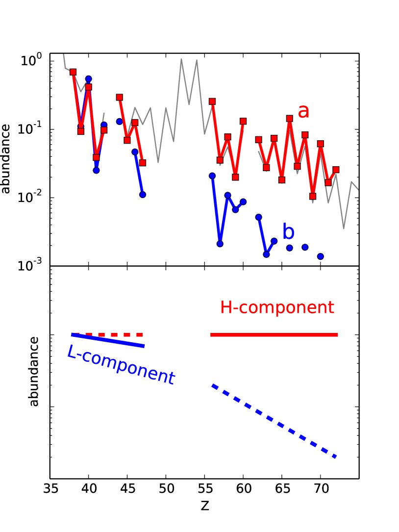
Figure 1.— Two metal-poor stellar abundance patterns are shown in the upper panel compared to the solar r process (grey thin line). The pattern “a” (red line and squares) corresponds to CS 22892-052, and the “b” pattern (blue line and circles) to HD 122563. All abundances are normalized to Sr. The bottom panel shows a sketch of the components that may contribute to produce these two patterns. The upper one is the H component (red line) and the lower one the L component (blue). The solid lines indicate that elements in this range are mainly produced by this component, while the dashed lines indicate that the component may not pay the predominant contribution to this elemental range.

This paper is organized as follows. The large sample of metal-poor stars from (Frebel et al., 2010) is reduced, homogenized, and discussed in detail in Sect. 2. In Sect. 3 the methods to obtain the H and L components are introduced and compared to observations. In Sect. 4 the separated L abundances are used to place constraints on a possible formation site; the neutrino-driven winds. Summary and conclusions can be found in Sect. 5.

2. Data—Observationally derived stellar abundances

To minimize the number of contributing processes, we only consider metal-poor (old) stars that are less enriched by s processes compared to younger (more metal-rich) stars. To clean the sample presented in Frebel et al. (2010), we apply five selection criteria (below) to the large, inhomogeneous sample:

1. $[$Fe/H$]<-2.5$: this cut removes the majority of the s-process contribution. Travaglio et al. (2004) state that the s process(es) contributes little to halo stars below [Fe/H]=$-1.5$. Recently, Hansen et al. (2014) found that the s process yields may be traceable below [Fe/H]=$-1.5$ possibly down to $-2.5$, but not lower. Hence, neglecting the s process below [Fe/H]$=-2.5$ is an observationally justified assumption. Including stars with a metallicity up to $-2.5$ (instead of staying below $-3$) ensures that a large fraction of heavy elements are still detectable, even if the star is not extremely enhanced in neutron-capture elements. Most absorption lines weaken as metallicity decreases, making the abundance analysis increasingly difficult with decreasing metallicity.

2. $[$C/Fe$]<0.7$: this ensures that no carbon enhanced metal-poor (CEMP) star is included (Aoki et al., 2007), as most Fe-poor stars are carbon-enhanced stars, many of which are also s-process enriched.

3. $[$Ba/Fe$]<1.0$: this cuts out Ba stars and together with the previous criteria removes strong s-process enhancement in, e.g., CEMP-s stars.

4. Excluding abundances that are only upper limits yields a better and more solid final abundance pattern with known reasonable sized uncertainties. This facilitates a more direct comparison of observations and predictions.

5. Most heavy elements are detected in the extended atmospheres of giant stars, that due to stellar evolution have had their surface composition altered. This change is normally seen in their carbon and nitrogen abundances, which is why we place the cuts: $[$C/N$]<-0.4$ and [N/Fe] $>0.5$. These exclude stars with internal mixing owing to the stellar evolution (Spite et al., 2005). Very evolved stars (giants) burn C into N and later O, which will result in lower C and higher N and O abundances.

The original sample from Frebel et al. (2010) is a compilation of different sources from the literature. Therefore, our reduced sample is inhomogeneous owing to the variety of different stellar parameter scales and methods used to derive these abundances. After carefully examining the observational data, inconsistencies between the “original” data found in the literature and the compilation in Frebel et al. (2010) were revealed for two of our reduced sample’s stars. As a consequence, these were removed from our final sample. The star CS 30325-094 (catalog ) has a Eu abundance that is observed only as an upper limit in François et al. (2007) and the Pm abundance was not found in the quoted reference. In addition, CS 22783-055 (catalog ) (McWilliam et al., 1995b, a) has abundances in the Frebel et al. 2010 table that we were not able to find in the literature.

If we also require that each star needs to have at least five heavy element detections or more (i.e., we do not count upper limits), the final reduced sample consists of 39 stars. However, if we loosen criteria (5) to only affect $[$C/N$]<-0.4$, and set no [N/Fe] constraint, the sample is increased to 53 stars (model 4 in Table 1).

The final abundance pattern of each star, consists of both neutral and ionized elemental abundances, and some species (e.g., Sr I—the minority of Sr) are more affected by nonlocal thermodynamic equilibrium (NLTE and possibly three-dimensional (3D)) effects than other species (e.g., Sr II—the majority of Sr). This introduces a possible bias between the mixture of neutral/ionized elements that compose the total abundance pattern, and this bias may exceed the uncertainties stemming from the inhomogeneity of the sample. The NLTE corrections are not calculated for all the heavy elements (owing to the lack of atomic physics), and even fewer of the heavy elements have NLTE corrections calculated for a large stellar parameter space (some of these elements are Sr and Ba which have been investigated in detail, e.g., Andrievsky et al. 2009, 2011; Bergemann et al. 2012; Hansen et al. 2013). Fortunately, several of the heavy elements have abundances derived from the majority species (which, in many cases, are single ionized lines), and for some of these elements the 3D and NLTE effects may cancel out, thereby removing the bias in the heavy element abundance pattern.

We account for the sample inhomogeneity that may lead to biases in the abundance pattern by propagating slightly increased uncertainties into the nucleosynthesis components in the next sections (Sect. 3 and Appendix A).

3. Nucleosynthesis components

Following Qian & Wasserburg (2001, 2007, 2008), we call the two components that contribute to the metal-poor stars the L component and H component (see Fig. 1 for schematic representation). We assume that the H component is the main source of heavy r process elements ($Z>50$), but it may also contribute to the lighter heavy elements ($38<Z<50$). In contrast, the L component contributes mainly to these lighter heavy elements, but may also extend toward the heavy $Z>50$ elements. With these two components, there are several possibilities to explain the typical patterns shown in the upper panel of Fig. 1. The pattern “a” can be produced only by an H component going from Sr to the heaviest elements. Another possibility to explain the “a” pattern would be a combination of an H component that contributes only to the heavy part ($Z>50$) and a L component to explain the pattern below $Z<50$. The “b” pattern can be the result of a single L component that extends toward heavy elements or the combination of an L component up to $Z=50$ and a small contribution from the H component to explain the low abundances of heavy elements.

3.1. Component identification

In order to explain the abundances of our reduced sample of stars described in Sect. 2 by an L and H component, we first extract the abundance pattern of these two components. The pure nucleosynthesis component patterns are obtained using three different methods (M1, M2, M3) in order to test their robustness and to estimate their uncertainties (see Appendix A for details). All methods use abundances from the metal-poor stars HD 122563 and HD 88609 (which have large [Sr/Eu] ratios, Honda et al. 2007) and CS 22892-052 (which has a large [Eu/Fe] ratio, Sneden et al. 2003).

Method one (M1) assumes that HD 122563 has only been enriched by the L component (due to the large Sr-enrichment) while CS 22892-052 (catalog ) has only been enriched by the H component (due to its large Eu-enrichment). As such, their abundances already show the individual components. These are shown in the upper panel of Fig. 2.

Method two (M2) follows Montes et al. (2007) and assumes that while CS 22892-052 (catalog ) has a pure H-component abundance, HD 122563 (catalog ) shows a large L component combined with a small H-component contribution. This small contribution is removed by subtracting the abundances of CS 22892-052 (catalog ) from the HD 122563 (catalog ) abundance (by scaling to the average of Eu, Gd, Dy, Er, and Yb abundances in each star). This leaves only the pure L-component pattern as shown in the middle panel of Fig. 2.

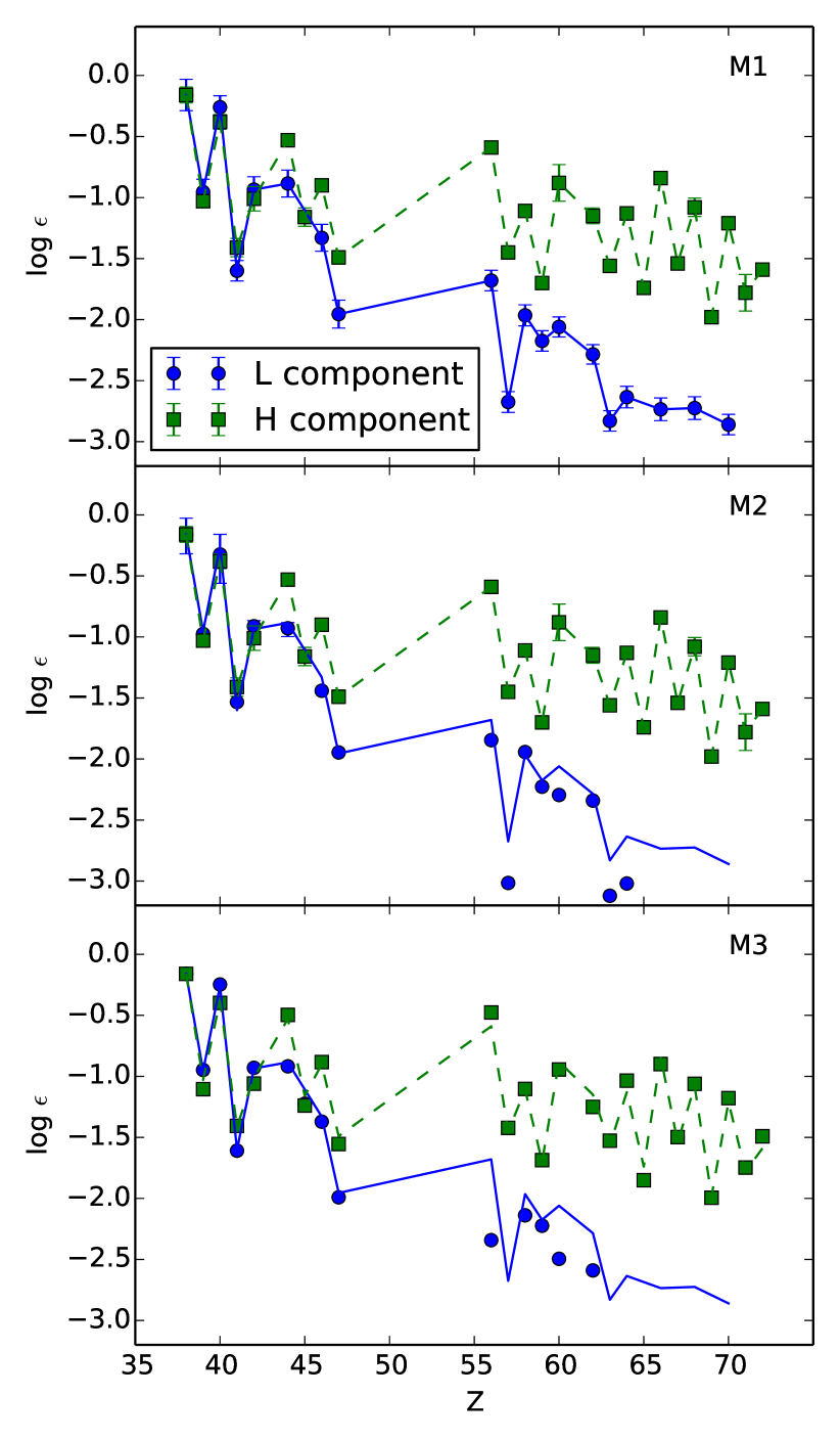
Figure 2.— Pure L component and H component obtained using the three methods described in the text. In all three panels, the solid blue (dashed green) line corresponds to the L(H) component obtained in method 1 (M1), while the symbols vary with the methods.

Method three (M3) follows Li et al. (2013) and assumes that the mentioned metal-poor stars’ abundances do not have pure nucleosynthesis components, but instead have a dominant contribution from one of the components. The pure component abundances are obtained by systematically eliminating the abundances from the process that contributes the least. The first-order L-component abundance is obtained by subtracting the CS 22892-052 abundances (scaled to the Eu abundance which is predominantly produced by the H component) from the average of the HD 122563 and HD 88609 (catalog ) abundances. Conversely, the first-order H-component abundance is obtained by subtracting the average of the HD 122563 and HD 88609 abundances (scaled to the Fe abundance) from the CS 22892-052 abundances. The individual components are obtained by further subtraction of the remaining contribution, e.g., the $n^{th}$-order L-component abundance is obtained by subtracting the $(n-1)^{th}$-order H-component abundances scaled to Eu from the average of the HD 122563 (catalog ) and HD 88609 (catalog ) stellar abundances. The procedure is repeated until the differences in both the L component and H component are smaller than the observational error. Figure 2 (bottom panel) shows the nucleosynthesis components obtained following this method. The robustness of the derived components using method three was checked by using different combinations of metal-poor stars. Since the assumption is that all stellar abundances at low metallicity have contributions from robust L and H components, any pair of metal-poor stars could, in principle, be used to obtain the pure components (see Appendix A for additional tests). However, the errors of the iterative method are smaller when the differences between the observed abundances are larger.

The derived H-component abundances shown in Fig 2 are remarkably consistent between the different methods. The calculated abundance difference between methods is within $\pm 0.2$ dex for every element. In contrast, the derived L-component abundances vary up to an order of magnitude for elements heavier than Ba. For elements between Sr and Ag, the obtained L-component abundances are within $\pm 0.2$ dex for all methods. In the following, we assume that both components have an uncertainty of $\pm 0.2$ dex for every element and consider the possibility, that the L component may be limited to elements up to Ag (see Sect. 3.2). Furthermore, we assume that the components are “robust” within the abundance uncertainties. This is a fair assumption for the H component, but may not be true for the L component as shown in Fig. 3. The stars presented in this figure have a typical L-component pattern that is fairly consistent (within $\sim 0.2$ dex) for Z$<$50. However, we refer to Sect. 4.1 and Fig. 10 for further discussion on the robustness of the L component. We stress that the robustness of the L component is an assumption that we will test in the following sections.

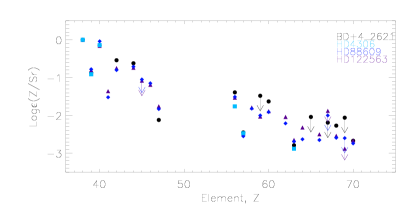
Figure 3.— Abundances normalized to Sr for four well-known L-component stars.

3.2. Fitting observations with two components

The H and L components introduced in the previous section are assumed to be responsible for the abundances ($Y$) of metal-poor stars. For every element with $Z>50$, the abundance of the sample stars can be expressed as a combination of these components ($Y_{H}$ and $Y_{L}$):

$$Y_{calc}(Z)=\big{(}C_{H}Y_{H}(Z)+C_{L}Y_{L}(Z)\big{)}\times 10^{[\mathrm{Fe/H}]},$$ (1)

where $C_{H}$ and $C_{L}$ are the weights of the H and L components to the abundances of the star, respectively. It should be noted that since there is an arbitrary scaling factor when defining $Y_{H}(Z)$ and $Y_{L}(Z)$, the values of $C_{H}$ and $C_{L}$ are relative and only their overall trends have physical significance. The factor $10^{[\mathrm{Fe/H}]}$ is introduced to normalize the abundances at different metallicities.

In order to find the coefficients $C_{H}$ and $C_{L}$ that best match the observationally derived abundances in metal-poor stars, the following $\chi^{2}$-distribution was minimized,

$$\chi^{2}=\frac{1}{\nu}\sum_{Z_{\mathrm{range}}}\big{(}\log Y_{\mathrm{observed}}(Z)-\log Y_{\mathrm{calc}}(Z)\big{)}^{2}/\Delta(Z)^{2},$$ (2)

where Z_range is the elemental range considered in the minimization, $\Delta(Z)$ corresponds to the abundance uncertainty of element $Z$ from both the observation and the nucleosynthesis component determination, and $\nu$ is the number of degrees of freedom in the fit (number of elements observed in Z_range minus the number of fitted coefficients $C$). The uncertainty in the observation (0.25 dex) and the intrinsic error in the component estimation (0.2 dex) were added in quadrature to obtain $\Delta$(Z) = 0.32 dex for all elements, see Appendix A.

Once the $\chi^{2}$-distribution (Eq. (2)) has been minimized for a given star, the minimum $\chi^{2}$ obtained with the preferred $C_{H}$ and $C_{L}$ coefficients is associated with that star. A star that has its abundances well (badly) calculated within this approach, would result in a low (high) $\chi^{2}$ value. A large number of stars with high $\chi^{2}$ values would indicate that the assumptions in our approach are incorrect.

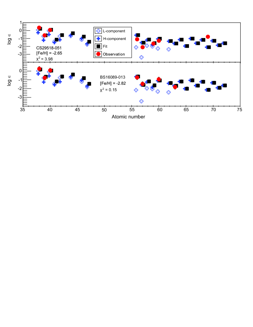
Figure 4.— Poor (top) and good (bottom) $\chi^{2}$ fit to two sample stars.

We calculate the $\chi^{2}$-distribution (Eq. (2)) for the stars in our sample. We have studied various models that assume different elemental ranges for every component and use M3 for the H component and vary the method for the L component. These models are summarized in Table 1. In model 4, the number of stars in the sample is larger and marked with an asterisk to indicate that stars in this model fulfill criteria 1 to 4, but not 5 (the criteria are described in Sect. 2).

Stars with low $\chi^{2}$ values show a typical trend (an example of this is shown in the lower panel of Fig. 4): Z$\geq$56 abundances fitted by the H component, and 38$\leq$Z$\leq$47 abundances fitted by a combination of L and H components. Thus, using the L component resulting from different methods has no effect on the fit because variations among methods are significant only for elements with $Z>50$. In addition, in the range 38$\leq$Z$\leq$47, the H- and L-component abundances are remarkably similar and within the error bar $\Delta$(Z) used in the fit. Since the L component is not making significant contributions to Z$>56$ (as can be seen from the good fits using models 1 and 2) a combination of L- and H-component contributions in the range of 38$\leq$Z$\leq$47, is almost equivalent to having a single process making only those abundances (Z$\leq$47) independently of the process responsible for the Z$\geq$56 abundances (model 3 in Table 1).

Table 1Details (component, sample size, and $\chi^{2}$) of the four models.

	H-	L-	Num. of	Stars with
model	component	component	stars in sample	$\chi^{2}\geq\chi^{2}_{5\%}$
1	M3	M3	39 stars	$<$1%
2	M3	M1	39 stars	$<$1%
3	M3, Z$>$47	M3, Z$<$56	39 stars	$<$1%
4	M3	M3	53 stars∗	11%

In order to test how well our models fit the stellar abundances, the expected $\chi^{2}$-probability distribution was calculated by adding up the expected $\chi^{2}$-distribution of every star considered. Each star has an expected $\chi^{2}$-distribution that depends only on the degrees of freedom. The expected $\chi^{2}$-probability distribution can thus be expressed as

$$f(\chi^{2})=\sum_{i}\frac{\nu_{i}}{2^{\nu_{i}/2}\Gamma(\nu_{i}/2)}e^{-\chi^{2}\nu_{i}/2}(\chi^{2}\nu_{i})^{(\nu_{i}/2-1)},$$ (3)

where $\nu_{i}$ is the number of degrees of freedom for star $i$. The $\chi^{2}$ test relies on the assumption that each elemental abundance is normally distributed within a given error. If the expected $\chi^{2}$-probability distribution is too large compared to the minimum $\chi^{2}$ values satisfying Eq. (2), we either conclude that a statistically improbable excursion of $\chi^{2}$ has occurred, or that our model is incorrect. If, on the other hand, the expected $\chi^{2}$-probability distribution is too small, it is not indicative of a poor model, but that a statistically improbable excursion of $\chi^{2}$ has occurred, or that $\Delta$(Z) has been overestimated in the model.

The minimum $\chi^{2}$ is shown as a function of metallicity in the right panel of Fig. 5 for the first three models listed in Table 1. In the left panel, one can see the expected $\chi^{2}$-distribution using Eq. (3) (red line) and histograms of the $\chi^{2}$-distribution values based on models 1, 2, and 3 in Table 1. The stellar sample contains only stars with at least five elemental abundance detections in the range Z$\geq$38. This guaranteed that the fit had at least three degrees of freedom after $C_{H}$ and $C_{L}$ were fitted. The total number of stars satisfying these restrictions combined with the five criteria outlined in Sect. 2 is 39 stars.

Figure 5.— Minimum $\chi^{2}$ values as a function of metallicity are shown in the right panel. Left panel shows expected $\chi^{2}$-distribution using Eq. (3) (red line) and histograms of the $\chi^{2}$-distribution values for different models presented in Table 1. Model 1 is shown as a solid line (left panel) and black solid circles (right panel), model 2 as a dashed line (left panel) and red open circles (right panel), and model 3 as a dotted line (left panel) and black open squares (right panel).

In order to test if the model is valid, we compare the number of stars with a $\chi^{2}$ value outside the range, where we expect to find 95% of the stars (stars with $\chi^{2}\geq\chi^{2}_{5\%}=2.31$). If that number of stars is much larger than 5% of the number of stars considered (in our sample that would correspond to 2 stars out of 39), it would indicate that our assumptions are incorrect. The three models considered are well within the expected $\chi^{2}$-probability distribution (see Fig. 5 and Table 1). Only 1 star, CS 22189-009 (catalog ), is outside the expected range of $\chi^{2}$ values. Therefore, this star cannot be explained by our assumption of two robust components. We have also tested an increment in the minimum number of elements observed. When this number is increased to $\geq$9 (reducing the sample to 21 stars), all stars have low $\chi^{2}$ values. The good agreement gives credence to the assumption of two independent robust processes being responsible for Z$\geq$38 abundances in most but not all stars.

The elemental range of the two components is tested in model 3 (Table 1). Here we obtain good fits when using the M3-H-component only for Z$>$47 and the M3-L-component only for Z$<$56 abundances. Without any overlap in the components a good fit is still obtained for 38 out of the 39 stars considered (see dotted line in the left panel of Fig. 5 and black open squares in the right panel). Therefore, using our method it is not possible to constrain the elemental range of the components.

We note, that if the criteria of excluding stars with internal mixing (Sect. 2) is removed (model 4, Table 1), the number of stars with $\chi^{2}$ values larger than $\chi^{2}_{5\%}\geq 2.31$ increases to six stars: CS 29518-051 (catalog ) (see Fig. 4), CS 22189-009 (catalog ), CS 22169-035 (catalog ), CS 30325-094 (catalog ), CS 30322-023 (catalog ), and CS 22783-055 (catalog ). Hence, internal mixing of the giant stars will show a clear effect in the overall abundance pattern, which is detectable using this method.

Generally, we obtained good fits to the observations assuming two dominant, robust components, but we can neither prove nor refute the presence of more processes nor can we at this state demonstrate the robustness of the processes. The good $\chi^{2}$ indicates that two processes could be sufficient and we discuss further in Sect. 4.1 the possible number of primary processes and their robustness.

4. Results and applications of the method

4.1. The star-to-star scatter

It is well known from earlier studies (see e.g., Spite & Spite, 1978; Truran, 1981; McWilliam et al., 1995b; Ryan et al., 1996; Fulbright, 2002; Barklem et al., 2005; François et al., 2007; Roederer et al., 2010; Hansen et al., 2012; Yong et al., 2013; Roederer et al., 2014) that a large star-to-star abundance scatter as a function of metallicity exists for most neutron-capture elements. The large abundance scatter has been attributed to the elements being produced in more than one type of nucleosynthesis process or astrophysical environment. For example, an $\alpha$ element like Mg does not show a large star-to-star scatter, but only spreads around a mean value of $\sim 0.34\pm 0.24$ dex, while many neutron-capture elements show a scatter of $\pm\sim 0.3$ to $1$ dex or even more (see Fig. 6 and Table 2). This scatter is much too large to be explained by observational biases or model assumptions (such as one-dimensional (1D) and LTE). In this section, we use the derived L and H components to split the observationally derived abundances into their individual contributions and show that even though this scatter is reduced, the scatter is still not completely removed in the individual components.

Figure 6.— Top: [Mg/Fe], middle: [Sr/Fe], and [Ba/Fe], bottom: [Eu/Fe]—all plotted versus [Fe/H]. A gray band around the average abundance indicates the star-to-star abundance scatter (standard deviation) for the full sample, while the dashed lines show the standard deviation for our sample. The values are given in Table 2.

Figure 6 shows the abundances of the stellar sample obtained by applying our selection criteria (Sect. 2) compared to the complete sample as a function of metallicity for a few selected elements. Just by applying the selection criteria the star-to-star scatter has decreased (see Table 2) and the selection criteria is therefore successful in removing most of the contamination originating from multiple processes as well as CEMP stars.

Table 2The mean and standard deviation for our sample and the full un-cut sample.

	$<$[Mg/Fe]$>$	$<$[Sr/Fe]$>$	$<$[Zr/Fe]$>$	$<$[Ba/Fe]$>$	$<$[Eu/Fe]$>$
Sample	0.34 $\pm$ 0.18	0.05 $\pm$ 0.34	0.22 $\pm$ 0.32	-0.12 $\pm$ 0.58	0.55 $\pm$ 0.66
Total	0.34 $\pm$ 0.24	0.10 $\pm$ 1.03	0.55 $\pm$ 1.33	-0.02 $\pm$ 0.78	0.47 $\pm$ 1.22

Figure 7.— Individual process contribution from the H component and L component to [Sr*, Zr*, Ba*, and Eu*/Fe] as a function of [Fe/H] from the top to the bottom. The L component is shown as filled blue diamonds, while the H component is depicted as filled red squares.

To fully understand the remaining star-to-star scatter present in the reduced stellar sample, we rewrite the standard [X/Fe] abundance convention to only include the contribution from either the L component ([X_L*/Fe] – Eq. 4) or the H component ([X_H*/Fe] – Eq. 5). The first logarithmic term in those equations corresponds to the total (normal) $\log\epsilon(X)$.

$$[X_{L}^{*}/\mathrm{Fe}]= \log(10^{\log\epsilon(X)}-(Y_{H}(X)\cdot C_{H}\cdot 10^{[\mathrm{Fe/H}]}))$$

$$-\log\epsilon(X)_{\odot}-[\mathrm{Fe/H}]$$ (4)

$$[X_{H}^{*}/\mathrm{Fe}]= \log(10^{\log\epsilon(X)}-(Y_{L}(X)\cdot C_{L}\cdot 10^{[\mathrm{Fe/H}]}))$$

$$-\log\epsilon(X)_{\odot}-[\mathrm{Fe/H}]$$ (5)

Table 3Mean $\pm$ standard deviation

	[Sr∗/Fe]	[Zr∗/Fe]	[Ba∗/Fe]	[Eu∗/Fe]
L	$-0.17\pm 0.32$	$0.04\pm 0.33$	$-1.03\pm 0.9$	$-0.46\pm 1.02$
H	$-0.44\pm 0.49$	$-0.36\pm 0.55$	$-0.15\pm 0.60$	$0.51\pm 0.54$

The L- and H-component contributions to the total abundance are shown in Fig. 7 as a function of [Fe/H]. Starting with the top panel showing [Sr^∗/Fe], we conclude that in most cases the L component contributes the most to the Sr abundance derived from observations of these stars. Only in a few stars, the H component contribution is larger. Table 3 shows the mean and standard deviation from the mean for the elements shown in Fig. 7. While Zr behaves similar to Sr (L component creating most of the observed abundance), both Ba and Eu are dominated by the H component. A large scatter is found for Ba and Eu vs. [Fe/H] and it indicates that these two n-capture H-component elements are not co-produced with Fe (as originally postulated in Spite & Spite, 1978). The standard deviation increases the more the formation process of the element in the numerator differs from that of the element in the denominator.

The situation for the lighter elements, Sr and Zr, is less clear cut because the larger scatter in these elements has the same size as the adopted uncertainty ($\pm$0.32 dex). Even though definite conclusions are not possible, it should be noted that both Qian & Wasserburg (2008) and Li et al. (2013) proposed an L-component extending down to iron-peak nuclei, so some co-production of Sr and Zr with Fe is possible. This partial co-production would reduce the scatter compared to completely uncorrelated nuclei such as Eu. Hence, this could point toward more than two formation processes contributing to the region ($38<Z<50$) or that the processes are less robust.

The robustness of the L- and H-component contributions can be studied in Fig. 8 and Fig. 9. Barium and Eu show an almost perfect correlation for the H component with little spread ($\pm 0.19$ dex). This confirms the robustness of the H component, which is in good agreement with the universality of the r process (the most likely process behind the H component) shown in many other studies (e.g. Cowan et al. 2002; Sneden et al. 2003). Strontium and Zr, on the other hand, show a larger star-to-star scatter in both L and H components, with standard deviations of 0.27 dex and 0.38 dex, respectively. Even though the deviations are at the limit of the component uncertainties ($\pm$0.32 dex), this suggests that the H component dominates the heavier elements (Z$\geq$56), and that it has a smaller intrinsic scatter compared to the L component’s intrinsic scatter. The relatively speaking larger scatter of the L component may indicate that the component/process is only robust within a $\pm 0.32$ dex uncertainty, or that there may be additional nucleosynthesis components/processes hiding wihtin this uncertainty. The method and current level of abundance accuracy do not allow us to distinguish between these possibilities.

Figure 8.— The calculated contribution from the L component ($Y_{L}$ blue, diamonds) and the main H component ($Y_{r}$ red, squares) for Sr and Zr.

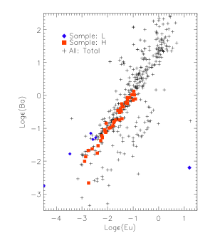
Figure 9.— The L- and H-calculated abundances for Eu and Ba. Details can be found in the legend.

By extracting stars from our sample with large L-component coefficients, we find strongly L-component-enriched stars to further test the robustness of the process. Figure 10 shows the stellar abundances of HE0104-5300 (catalog ), HE0340-5355 (catalog ), BS16469-075 (catalog ), HE1252-075 (catalog ), HE2219-0713 (catalog ), BD+4_2621 (catalog ), HD4306 (catalog ), HD88609 (catalog ), and HD122563 (catalog ) which have a predominant L-component contribution. They show a larger spread in their abundance pattern than first expected (see Fig. 3, where the well-known L-component stars agree within $\pm 0.2$ dex for every element). The larger sample of possible L-dominated stars indicate that these show an abundance spread within $\pm 0.32$ dex, which is the allowed abundance uncertainty adopted for our pattern fitting (see Fig. 10). The increase in the abundance spread could indicate we need to classify the L-component stars such as HD122563 (catalog ) and HD88609 (catalog ) better, to distinguish between such stars and the others shown in Fig. 10. Alternatively, the L-dominated stars actually span a wider range of abundances than H-dominated (e.g., the r-II) stars do, and the assumed robustness of the L component may break down. If this is the case, this would allow for a wider range of astrophysical conditions facilitating the process or for several processes to coexist and blend into our L component thereby increasing the scatter to 0.32 dex.

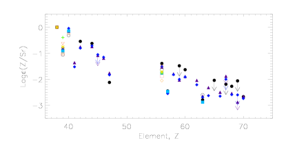
Figure 10.— Abundances normalized to Sr for L-component stars and candidate stars with promising L-component patterns.

Recently, Roederer (2013) showed an almost perfect correlation between Sr and Ba and concluded that all stars must have heavy elements in their atmospheres.The reason why we do not detect them is due to weak lines and observational biases. In Fig. 11, we show that both Sr and Ba grow ( as in, e.g., Aoki et al. (2005); Roederer (2013)), almost at the same rate. This could indicate a coproduction of Sr and Ba in the same site or that the nucleosynthesis processes create both elements in almost the same amounts. However, the large star-to-star scatter could veil differences in the formation process and/or site between Sr and Ba. Accurate isotopic abundances for both elements in a large sample are needed to settle this issue. Currently, only Ba has been studied on an isotopic level in small samples (see, e.g., Roederer et al. 2008; Gallagher et al. 2012 and references therein). Only when splitting the Sr and Ba abundances into components we detect the differences in the single formation processes (for comparison see Figs. 8 and 9). This separation method is currently the best proxy for isotopic abundances. We clearly see the difference in how Sr is predominantly produced by an L-component process, a process which does not have to produce any or only little Ba (see Figs. 7–11). This separation into L- and H-components partially detaches the origin of these two elements as they can be produced in different ratios in each component/process. The relation showed in Fig. 11 indicates that despite the fact that all stars have most likely been enriched in heavy elements, they do not need to be created by the same process, but could originate from the same object via different processes or have been mixed from different sites prior to incorporation. This statement will need to be verified in the future by improved yield predictions as well as GCE models, which will help us disentangle the formation sites and physical quantities.

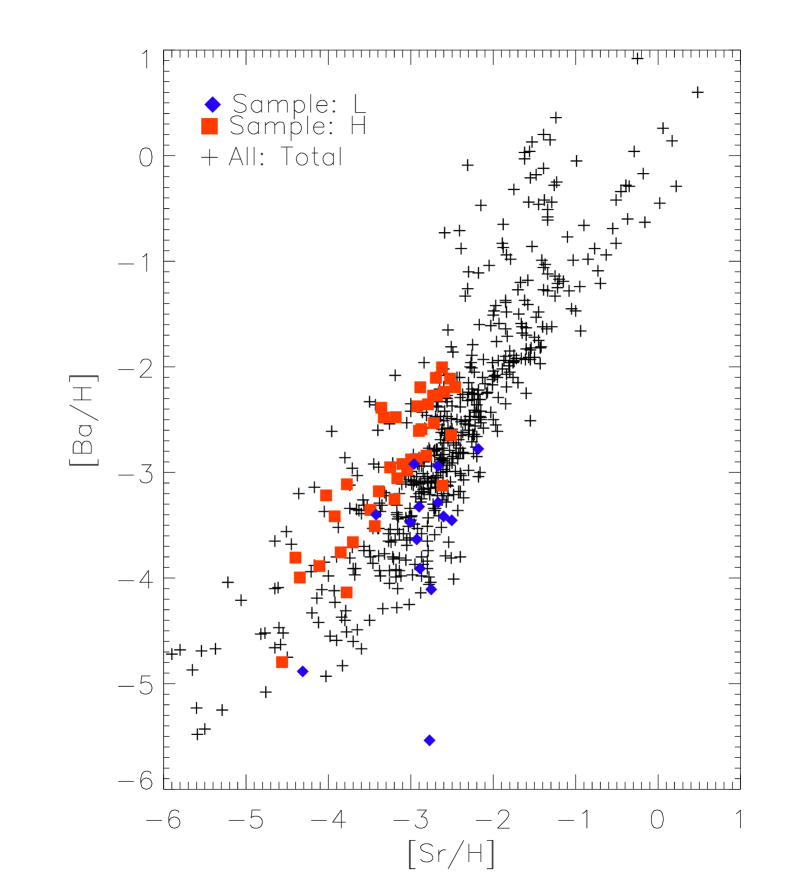
Figure 11.— Log$\epsilon$ abundances of Sr vs. Ba. The contributions from the L component (diamonds) and the H component (main r process) are over plotted (squares).

4.2. Predicting abundances

Europium is an important element because it is almost a pure r-process tracer. Thus, we need to know how this element behaves observationally at the lowest metallicities to constrain and optimize theory.

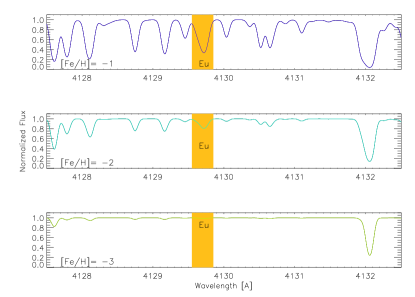
Figure 12.— Three synthetic spectra of giant stars with the same stellar model parameters (T=5200K, $\log g$= 2.0), but three different metallicities: [Fe/H]= $-1,-2$, and $-3$ in the top, middle, and bottom panels, respectively. This shows the effect of metallicity on the Eu line strength (still detectable at [Fe/H]$=-2.5$), and the difficulties in detecting the very weak Eu lines at [Fe/H]$\leq-3$.

Figure 12 shows that it is very challenging (or impossible) to measure Eu abundances in extremely and hyper metal-poor stars (which confirms the bias mentioned in Roederer 2013). This is a problem because the Eu abundances are needed to compute abundance patterns and to improve results and interpretations from, e.g., galactic chemical evolution (GCE) models. These models rely on the number (statistics) of the observationally derived abundances. Our method may help improve the statistics for future GCE models of Eu.

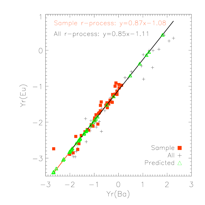
Figure 13.— H-component fraction of the $\log\epsilon$ abundances of Ba and Eu for the selected sample (filled red squared), for all stars with calculated components (black plusses), and predicted Eu abundances (green triangles). Lines have been fitted to the selected sample as well as all stars with calculated components.

Since 94% of Eu is created by the r process/H component (see e.g., Bisterzo et al., 2014), one can use the described method (Sect. 3) to predict Eu abundances, which cannot be derived from observations owing to the very weak absorption lines found at low-metallicity (or poor quality) spectra. By assuming that Eu is purely created in the H component, Eu can be calculated via a scaling relation between the H component’s Eu and Ba abundances. Barium is an obvious choice because this element is a good H-component tracer at low metallicity and it shows fairly strong absorption lines even in extremely metal-poor stars. Therefore, we know the Ba abundance in a much larger number of stars than the ones for which we know the Eu abundance (see Fig. 6).

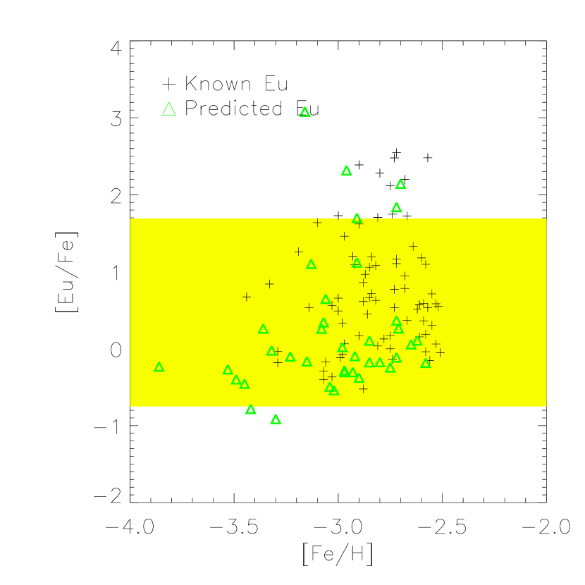
Figure 14.— [Eu/Fe] as a function of [Fe/H]. (Observationally derived Eu shown as pluses.) The predicted, i.e., not observationally detectable main H component [Eu/Fe] vs, [Fe/H] (green triangles). The yellow band is the standard deviation as shown in Fig. 6.

The relation between the H component Eu and Ba (see Fig. 13) can be then used to predict ‘unobserved’ Eu abundances (triangles in the figure):

$$\log\epsilon({\mathrm{E}u})_{r}=0.87\cdot\log\epsilon(\mathrm{Ba})_{r}-1.08.$$ (6)

By using this relation, the number of Eu abundances known below [Fe/H] =$-2.5$ would increase by 50%. Moreover, the predicted [Eu/Fe] abundances as a function of metallicity are shown in Fig. 14 and follow the observationally derived abundances. This indicates that within the assumption that the method produces reasonable Eu abundances, which for most stars are trustworthy, but it cannot predict accurate abundances for stars such as the outliers mentioned in Sect. 3.2.

Although, this method can by no means replace real observationally derived abundances, it can be used to estimate, e.g., Eu abundances either for GCE calculations or to estimate stellar abundances when applying for follow-up observing time.

4.3. Using components to constrain astrophysics

In this section, we use the derived L-component abundances to constrain the astrophysical conditions of one of the possible sites where this component may be produced: neutrino-driven winds in core collapse supernovae. Similar studies have been carried out for the r process (see, e.g., Mumpower et al. (2012)).

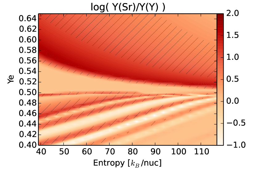
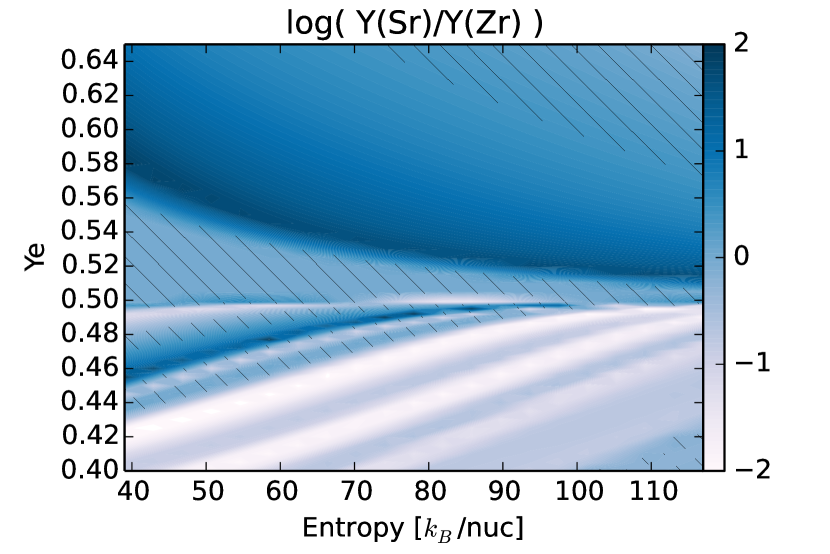
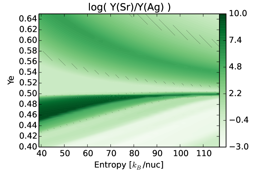
Figure 15.— Ratios of abundances for Sr and Y (upper panel), Sr and Zr (middle panel), and Sr and Ag (bottom panel) are shown in logarithmic scale for different entropies and $Y_{e}$. In the hatched regions the ratios agree with the ones of the L component $\pm$0.32.

Neutrino-driven winds occur after a successful core-collapse supernova explosion, when neutrinos deposit their energy in the outer layers of the neutron stars, and this layer gets ejected (see Arcones & Thielemann (2013) for a recent review). Although neutrino-driven winds were thought to be the site for the r process (Woosley et al., 1994), recent hydrodynamic simulations have shown that the required extreme conditions are not reached. It is still possible that the winds may have the conditions necessary to produce the L-component conditions as have been explored in Arcones & Montes (2011).

To explore under which astrophysical conditions in neutrino-driven winds are capable of reproducing the L-component abundances, we have systematically modified a wind trajectory from Arcones et al. (2007). This trajectory corresponds to an explosion of a 15 $M_{\odot}$ progenitor based on Newtonian hydrodynamic simulations with a simple neutrino transport. The simplification in the transport makes it possible to study the evolution from a few milliseconds up to few seconds post bounce for various progenitors and explosion energies in one and two dimensions (for more details see Arcones et al. (2007); Arcones & Janka (2011)). The approximations in the simulations may lead to small variations of the wind parameters such as expansion timescale, entropy, and electron fraction compared to what was obtained in the original trajectory. In order to account for the uncertainty in the wind parameters, we systematically varied them within their expected uncertainty. To explore different entropies ($S\propto T^{3}/\rho$), the density was reduced and increased within $\sim\pm 30$%. The initial electron fraction was also varied from neutron- to proton-rich conditions. Different expansion timescales were explored by taking slower and faster trajectories obtained in the same simulation at different times.

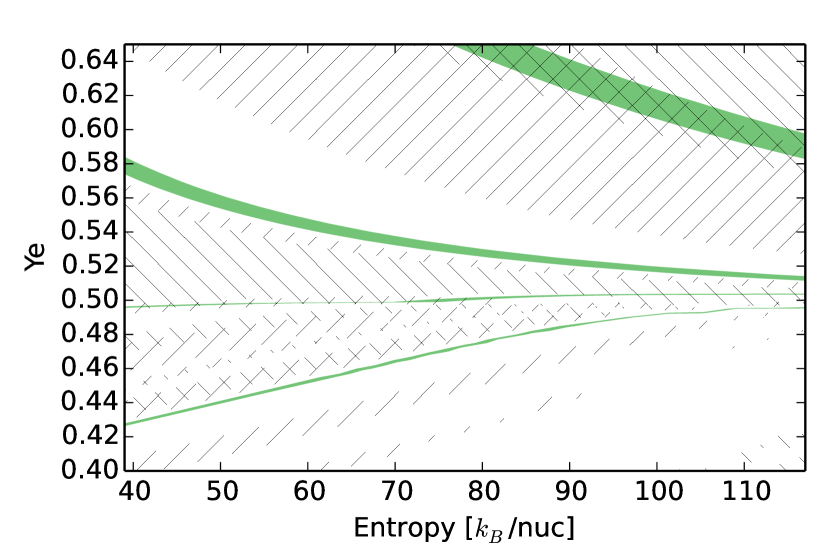
Figure 16.— L component predicts the ratio of the abundances for Sr/Y, Sr/Zr, and Sr/Ag within some error bars. This figure shows the wind parameter space and the regions where the ratios Sr/Y ($//$), Sr/Zr ($\setminus\setminus$), and Sr/Ag (green) agree with the L-component predictions.

Figure 15 shows abundance ratios of Sr with respect to Y, Zr, and Ag using a wind trajectory ejected five seconds after bounce as a function of entropy and electron fraction. The calculated L-component ratios shown in Fig. 15 are: Sr/Y=6.13, Sr/Zr=1.22, and Sr/Ag=48.25. These values with their associated observational and statistical errors of the method ($\pm 0.32$ dex) correspond to the marked regions in the figures. Figure 16 shows the overlapping regions where all the simulated ratios (Sr/Y, Sr/Zr, and Sr/Ag) agree with the extracted L-component ratios. For very proton-rich conditions, there is a band where all ratios overlap. Such conditions ($Y_{e}\approx 0.62$ and $S\approx 100k_{\mathrm{B}}/\mathrm{nuc}$) may be achieved a few seconds after the explosion. Note that the abundances in proton-rich winds depend on the electron antineutrino luminosity and energy because the nuclei are produced by the $\nu p$ process (Pruet et al., 2006; Fröhlich et al., 2006; Wanajo, 2013). Slightly different antineutrino luminosities and energies may result in different entropies and electron fractions. Figure 16 also shows slightly different proton-rich conditions ($Y_{e}\sim 0.50-0.55$) that could reproduce the derived L-component abundances. However, this slightly proton-rich ($Y_{e}\sim 0.50-0.55$) region of the parameter space is less relevant because the abundances of elements between Sr and Ag for such conditions are very small. In neutron-rich ($Y_{e}<0.5$) conditions the L-component ratios can be reproduced only in a very narrow band of the parameter space. For small variations of the wind parameters the abundances change steeply in contrast to the smooth trend in proton-rich winds (Fig. 15 and Arcones & Bliss (2014)). During the time evolution of the wind, the parameters are likely to evolve and change. Therefore, given the very narrow range of neutron-rich conditions that can reproduce the L abundances, it is likely that a small change in the astrophysical conditions will result in a non-robust L component. If, on the other hand, the L component is robust (as assumed in this paper), proton-rich conditions are more feasible, since they allow for a wider range of astrophysical conditions and still explain the observed L abundances. All previous discussion is based on a single expansion timescale, we have also studied other trajectories varying this quantity and find that the qualitative behavior and conclusions are the same.

The parameters of the neutrino-driven wind evolve with time as the neutrino luminosity decreases and the neutron star contracts and cools. Variations are also expected for different stellar progenitors because more massive ones will lead to more massive neutron stars which, in turn, means higher entropy allowing heavier elements to form (Qian & Woosley, 1996; Otsuki et al., 2000; Thompson et al., 2001). Therefore, the contribution from neutrino-driven winds to the observed abundances and to the L component comes from combinations of wind parameters, i.e., various points in Figs. 15–16. In order to explain the L component, most of the mass needs to be ejected with parameters from the overlapping regions in Fig. 16, even if any combination of wind parameters can be realized. If the contribution from neutrino-driven winds comes from very different regions of the parameter space, the abundance pattern would not reproduce the L component and it would not be robust. Therefore, the robustness (within error bars) strongly constrains the astrophysical conditions where the L component is produced.

Which is the heaviest element that can be produced in neutrino-driven winds for typical wind parameters? For typical wind conditions, Ba is not produced or only in a negligible amount. Therefore, if observations confirm that the L component extends up to Ba, the neutrino-driven wind (as obtained in current hydrodynamic simulations) is not likely to be responsible for the L component.

5. Summary & Conclusion

Abundances from metal-poor stars provide clues about the origin of the elements in the early universe. We have used the large inhomogeneous sample of metal-poor stars from Frebel et al. (2010), after applying selection criteria to remove contamination from s-process abundances, self mixing, etc., to obtain abundances from single nucleosynthesis processes. By assuming only two nucleosynthesis processes (the H and L components following Qian & Wasserburg 2001) contribute to the metal-poor stellar abundances, and that each single event creates robust abundances (within $\pm 0.2$ dex), we propose that the observationally derived abundances in all metal-poor stars can be explained by a linear superposition of these two contributions. We have separated the abundances into single component contributions by different methods (M1, M2, and M3 in Sect. 3.1). The derived H-component abundances (commonly attributed to the r process) are remarkably consistent between the different methods (within $\pm 0.2$ dex for every element). In contrast, even though for elements between Sr and Ag the obtained L-component abundances are within $\pm 0.2$ dex among different methods, the abundances vary up to an order of magnitude for elements heavier than Ba.

For the vast majority of stars in our sample, we have shown that these two robust components are enough to explain the stellar abundance patterns. A similar conclusion was also reached by Li et al. (2013) using a different stellar sample. Most stars have abundances that are well reproduced by adding up the L and H components, and the abundances of elements $Z\geq 56$ are generally created by the H component, while the abundance of elements $38\leq Z\leq 47$ created by a combination of L and H components. Since the L component does not have a significant contribution to elements $Z\geq 56$, the exact L abundance to those elements (obtained by the different methods) does not change or affect the good agreement between our model and observationally derived abundances. In each method, we found one or a few outlying stars that could not be explained under our assumptions using this method. This could indicate that our method is incomplete or that our assumptions are too strong. However, these outliers (in model 4) seem to have been self-enriched due to internal mixing, which causes the poor $\chi^{2}$ values. The general good agreement between our simple analytical model and the metal-poor stellar abundances indicates that two robust nucleosynthesis processes are responsible for the abundances of almost all metal-poor stars considered here.

By deconvolving the stellar abundances into the individual components, we have also studied the star-to-star abundance scatter. Since the H component is mainly responsible for the $Z\geq 56$ abundances, most of the observed scatter, as a function of metallicity is also observed in the H contribution, and it indicates that Fe and the H component are not co-produced (as originally postulated in Spite & Spite 1978). The robustness of the H-component contributions was confirmed by studying the scatter between different H contributions ($<\pm 0.2$ dex – see Fig. 9). For elements $38\leq Z\leq 47$, the situation is not as clear since the observed scatter as a function of metallicity in the L component is similar to the total attributed uncertainty in our model ($\pm 0.32$ dex). The scatter between different L-elemental contributions was also at the limit of what was expected ($\pm 0.32$ dex). This, and the fact that the abundance pattern of stars with a relative large L-component contribution is larger than originally expected, suggests that the H component has a smaller intrinsic scatter compared to the L component’s intrinsic scatter. The relative larger scatter of the L component may either indicate that the process is robust only within a $\pm 0.32$ dex uncertainty or that there could be additional nucleosynthesis components or processes hiding within the allowed uncertainty. The method used in this paper does not allow us to distinguish between these possibilities.

We consider neutrino-driven winds in core-collapse supernovae as a possible site and use the derived L-component abundances to constrain the astrophysical wind conditions. In order to explain these abundances, the environment likely needs to be proton-rich within a significantly constrained parameter space. If the L component is not robust, or if a single event has evolving conditions, there are even narrower bands of the parameter space that can reproduce the observations. In addition, the neutrino-driven winds are not likely to create Ba or heavier elements. If future abundance observations of L-dominated stars show that Ba is likely to be produced in an L component, their abundances are not likely to be created in neutrino-driven winds in core-collapse supernovae. Both simulations and observations need to improve to further constrain the production of heavy elements and assess the robustness and number of processes working at low metallicity.

Appendix A Uncertainties from observations and models

To assess how accurate the method is in splitting the abundance contributions from the L and H components, we carried out several tests to answer two questions: (1) Does the outcome depend on the intial set of stars? (2) How do the observational uncertainties (either intrinsic or due to the inhomogeneous stellar sample) affect the derived abundances? For this purpose, we use a new set of stars that are neither predominantly L- or H-component enriched, and therefore we used method M3 because it does not assume a dominant process. BD+4_2621 (catalog ) and HD6268 (catalog ) were selected because these stars have detailed abundances for a large number of elements. The derivation of the L- and H-component abundances using these stars’ abundances is referred to as method M3b. The impact of the uncertainties on the observed stellar abundances and the inhomogeneity of the sample was tested by creating an extreme case based on BD+4_2621 (catalog ) (method M3c). The new abundances in this “modified” star were “created” by randomly selecting abundances for that specific star found in literature for each element (generally the literature values vary within the observational uncertainty). The abundances of other stars were not modified. Figure 17 shows the abundances obtained by using BD+4_2621 (catalog ) and HD6268 (catalog ) in method M3b, and using method M3c for the “modified” BD+4_2621 (catalog ) and HD6268 (catalog ). Similar results are obtained using different combinations of stars. All H- and L-component abundances in the range $38\leq Z\leq 47$ are very similar and show a good agreement within $\pm$0.2 dex. By comparing the results of methods M3b and M3c, it can be seen that the uncertainty in the abundance determination due to the observational uncertainty is on average within $\pm$0.25 dex for all elements. For L-component nuclei with $Z\geq 56$, the differences among the methods (M3, M3b, and M3c) are larger and this reflects the intrinsic limitations of the method (or physical features of the process, since the L component may not create these nuclei very efficiently). The more similar the abundances of the stars are, the larger the uncertainty in the decomposed abundances get. The difference between the methods can be taken as a conservative uncertainty in the component abundances, because BD+4_2621 (catalog ) are HD6268 (catalog ) are not dominated by an individual component (L or H). The uncertainty obtained based on M3, M3b , and M3c is similar to the one based on M1, M2, and M3. Therefore, the use of different L-component abundances (M1 and M2 in Table 1) also covers the error due to the choice of the initial stars.

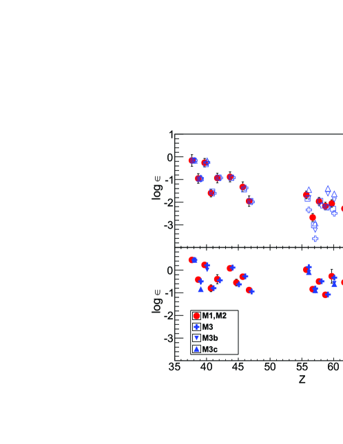
Figure 17.— M1, M2, M3 refers to the fitting methods described in Sect. 3 and the letters b and c indicate that BD+4_2621 and HD6268 were used instead of HD122563 and CS 22892-052.

Since the uncertainty for both components (excluding L component $Z\geq 56$) is within $\sim 0.2$ dex and the observationally derived abundances have on average 0.25 dex uncertainty, these contributions were added in quadrature, yielding a value of $\pm 0.32$ dex, and it is used in the abundance deconvolution described in the Sect. 3.2.

References

- Anders & Grevesse (1989) Anders, E. & Grevesse, N. 1989, Geochim. Cosmochim. Acta, 53, 197
- Andrievsky et al. (2011) Andrievsky, S. M., Spite, F., Korotin, S. A., François, P., Spite, M., Bonifacio, P., Cayrel, R., & Hill, V. 2011, A&A, 530, A105
- Andrievsky et al. (2009) Andrievsky, S. M., Spite, M., Korotin, S. A., Spite, F., François, P., Bonifacio, P., Cayrel, R., & Hill, V. 2009, A&A, 494, 1083
- Aoki et al. (2007) Aoki, W., Beers, T. C., Christlieb, N., Norris, J. E., Ryan, S. G., & Tsangarides, S. 2007, ApJ, 655, 492
- Aoki et al. (2005) Aoki, W., Honda, S., Beers, T. C., Kajino, T., Ando, H., Norris, J. E., Ryan, S. G., Izumiura, H., Sadakane, K., & Takada-Hidai, M. 2005, ApJ, 632, 611
- Arcones & Bliss (2014) Arcones, A. & Bliss, J. 2014, Journal of Physics G Nuclear Physics, 41, 044005
- Arcones & Janka (2011) Arcones, A. & Janka, H.-T. 2011, aap, 526, A160+
- Arcones et al. (2007) Arcones, A., Janka, H.-T., & Scheck, L. 2007, aap, 467, 1227
- Arcones & Montes (2011) Arcones, A. & Montes, F. 2011, ApJ, 731, 5
- Arcones & Thielemann (2013) Arcones, A. & Thielemann, F.-K. 2013, Journal of Physics G Nuclear Physics, 40, 013201
- Arnould et al. (2007) Arnould, M., Goriely, S., & Takahashi, K. 2007, Phys. Repts., 450, 97
- Barklem et al. (2005) Barklem, P. S., Christlieb, N., Beers, T. C., Hill, V., Bessell, M. S., Holmberg, J., Marsteller, B., Rossi, S., Zickgraf, F.-J., & Reimers, D. 2005, A&A, 439, 129
- Bauswein et al. (2013) Bauswein, A., Goriely, S., & Janka, H.-T. 2013, ApJ, 773, 78
- Beers & Christlieb (2005) Beers, T. C. & Christlieb, N. 2005, ARA&A, 43, 531
- Bergemann et al. (2012) Bergemann, M., Hansen, C. J., Bautista, M., & Ruchti, G. 2012, A&A, 546, A90
- Bisterzo et al. (2010) Bisterzo, S., Gallino, R., Straniero, O., Cristallo, S., & Käppeler, F. 2010, MNRAS, 404, 1529
- Bisterzo et al. (2011) —. 2011, MNRAS, 418, 284
- Bisterzo et al. (2014) Bisterzo, S., Travaglio, C., Gallino, R., Wiescher, M., & Käppeler, F. 2014, ApJ, 787, 10
- Burbidge et al. (1957) Burbidge, E. M., Burbidge, G. R., Fowler, W. A., & Hoyle, F. 1957, Rev. Mod. Phys., 29, 547
- Burris et al. (2000) Burris, D. L., Pilachowski, C. A., Armandroff, T. E., Sneden, C., Cowan, J. J., & Roe, H. 2000, ApJ, 544, 302
- Cowan et al. (1995) Cowan, J. J., Burris, D. L., Sneden, C., McWilliam, A., & Preston, G. W. 1995, ApJ, 439, L51
- Cowan et al. (2002) Cowan, J. J., Sneden, C., Burles, S., Ivans, I. I., Beers, T. C., Truran, J. W., Lawler, J. E., Primas, F., Fuller, G. M., Pfeiffer, B., & Kratz, K.-L. 2002, ApJ, 572, 861
- Cruz et al. (2013) Cruz, M. A., Serenelli, A., & Weiss, A. 2013, A&A, 559, A4
- Farouqi et al. (2010) Farouqi, K., Kratz, K.-L., Pfeiffer, B., Rauscher, T., Thielemann, F.-K., & Truran, J. W. 2010, ApJ, 712, 1359
- François et al. (2007) François, P., Depagne, E., Hill, V., Spite, M., Spite, F., Plez, B., Beers, T. C., Andersen, J., James, G., Barbuy, B., Cayrel, R., Bonifacio, P., Molaro, P., Nordström, B., & Primas, F. 2007, A&A, 476, 935
- Frebel et al. (2010) Frebel, A., Simon, J. D., Geha, M., & Willman, B. 2010, ApJ, 708, 560
- Freiburghaus et al. (1999) Freiburghaus, C., Rosswog, S., & Thielemann, F.-K. 1999, ApJ, 525, L121
- Frischknecht et al. (2012) Frischknecht, U., Hirschi, R., & Thielemann, F.-K. 2012, A&A, 538, L2
- Fröhlich et al. (2006) Fröhlich, C., Martínez-Pinedo, G., Liebendörfer, M., Thielemann, F.-K., Bravo, E., Hix, W. R., Langanke, K., & Zinner, N. T. 2006, Physical Review Letters, 96, 142502
- Fulbright (2002) Fulbright, J. P. 2002, AJ, 123, 404
- Gallagher et al. (2012) Gallagher, A. J., Ryan, S. G., Hosford, A., García Pérez, A. E., Aoki, W., & Honda, S. 2012, A&A, 538, A118
- Hansen et al. (2014) Hansen, C. J., Andersen, A. C., & Christlieb, N. 2014, A&A, 568, A47
- Hansen et al. (2013) Hansen, C. J., Bergemann, M., Cescutti, G., François, P., Arcones, A., Karakas, A. I., Lind, K., & Chiappini, C. 2013, A&A, 551, A57
- Hansen et al. (2012) Hansen, C. J., Primas, F., Hartman, H., Kratz, K.-L., Wanajo, S., Leibundgut, B., Farouqi, K., Hallmann, O., Christlieb, N., & Nilsson, H. 2012, A&A, 545, A31
- Hill et al. (2002) Hill, V., Plez, B., Cayrel, R., Beers, T. C., Nordström, B., Andersen, J., Spite, M., Spite, F., Barbuy, B., Bonifacio, P., Depagne, E., François, P., & Primas, F. 2002, A&A, 387, 560
- Hoffman et al. (1996) Hoffman, R. D., Woosley, S. E., Fuller, G. M., & Meyer, B. S. 1996, apj, 460, 478
- Honda et al. (2007) Honda, S., Aoki, W., Ishimaru, Y., & Wanajo, S. 2007, ApJ, 666, 1189
- Honda et al. (2004) Honda, S., Aoki, W., Kajino, T., Ando, H., Beers, T. C., Izumiura, H., Sadakane, K., & Takada-Hidai, M. 2004, ApJ, 607, 474
- Hotokezaka et al. (2013) Hotokezaka, K., Kyutoku, K., Tanaka, M., Kiuchi, K., Sekiguchi, Y., Shibata, M., & Wanajo, S. 2013, ApJ, 778, L16
- Just et al. (2014) Just, O., Bauswein, A., Ardevol Pulpillo, R., Goriely, S., & Janka, H.-T. 2014, ArXiv e-prints
- Korobkin et al. (2012) Korobkin, O., Rosswog, S., Arcones, A., & Winteler, C. 2012, MNRAS, 426, 1940
- Lai et al. (2008) Lai, D. K., Bolte, M., Johnson, J. A., Lucatello, S., Heger, A., & Woosley, S. E. 2008, ApJ, 681, 1524
- Lattimer & Schramm (1974) Lattimer, J. M. & Schramm, D. N. 1974, ApJ, 192, L145
- Li et al. (2013) Li, H., Shen, X., Liang, S., Cui, W., & Zhang, B. 2013, PASP, 125, 143
- Lucatello et al. (2005) Lucatello, S., Tsangarides, S., Beers, T. C., Carretta, E., Gratton, R. G., & Ryan, S. G. 2005, ApJ, 625, 825
- Martínez-Pinedo et al. (2012) Martínez-Pinedo, G., Fischer, T., Lohs, A., & Huther, L. 2012, Physical Review Letters, 109, 251104
- Masseron et al. (2010) Masseron, T., Johnson, J. A., Plez, B., van Eck, S., Primas, F., Goriely, S., & Jorissen, A. 2010, A&A, 509, A93
- McWilliam et al. (1995a) McWilliam, A., Preston, G. W., Sneden, C., & Searle, L. 1995a, AJ, 109, 2757
- McWilliam et al. (1995b) McWilliam, A., Preston, G. W., Sneden, C., & Shectman, S. 1995b, AJ, 109, 2736
- Metzger & Fernández (2014) Metzger, B. D. & Fernández, R. 2014, MNRAS, 441, 3444
- Montes et al. (2007) Montes, F., Beers, T. C., Cowan, J., Elliot, T., Farouqi, K., Gallino, R., Heil, M., Kratz, K., Pfeiffer, B., Pignatari, M., & Schatz, H. 2007, ApJ, 671, 1685
- Mumpower et al. (2012) Mumpower, M. R., McLaughlin, G. C., & Surman, R. 2012, Phys. Rev. C, 85, 045801
- Otsuki et al. (2000) Otsuki, K., Tagoshi, H., Kajino, T., & Wanajo, S. 2000, ApJ, 533, 424
- Perego et al. (2014) Perego, A., Rosswog, S., Cabezón, R. M., Korobkin, O., Käppeli, R., Arcones, A., & Liebendörfer, M. 2014, MNRAS, 443, 3134
- Pignatari et al. (2008) Pignatari, M., Gallino, R., Meynet, G., Hirschi, R., Herwig, F., & Wiescher, M. 2008, ApJ, 687, L95
- Pruet et al. (2006) Pruet, J., Hoffman, R. D., Woosley, S. E., Janka, H.-T., & Buras, R. 2006, ApJ, 644, 1028
- Qian & Wasserburg (2007) Qian, Y. & Wasserburg, G. J. 2007, physrep, 442, 237
- Qian & Wasserburg (2008) —. 2008, ApJ, 687, 272
- Qian & Wasserburg (2001) Qian, Y.-Z. & Wasserburg, G. J. 2001, ApJ, 559, 925
- Qian & Woosley (1996) Qian, Y.-Z. & Woosley, S. E. 1996, ApJ, 471, 331
- Roberts et al. (2012) Roberts, L. F., Reddy, S., & Shen, G. 2012, Phys. Rev. C, 86, 065803
- Roederer (2013) Roederer, I. U. 2013, AJ, 145, 26
- Roederer et al. (2010) Roederer, I. U., Cowan, J. J., Karakas, A. I., Kratz, K.-L., Lugaro, M., Simmerer, J., Farouqi, K., & Sneden, C. 2010, ApJ, 724, 975
- Roederer et al. (2008) Roederer, I. U., Lawler, J. E., Sneden, C., Cowan, J. J., Sobeck, J. S., & Pilachowski, C. A. 2008, ApJ, 675, 723
- Roederer et al. (2014) Roederer, I. U., Preston, G. W., Thompson, I. B., Shectman, S. A., Sneden, C., Burley, G. S., & Kelson, D. D. 2014, AJ, 147, 136
- Ryan et al. (1996) Ryan, S. G., Norris, J. E., & Beers, T. C. 1996, ApJ, 471, 254
- Sneden et al. (2008) Sneden, C., Cowan, J. J., & Gallino, R. 2008, araa, 46, 241
- Sneden et al. (2003) Sneden, C., Cowan, J. J., Lawler, J. E., Ivans, I. I., Burles, S., Beers, T. C., Primas, F., Hill, V., Truran, J. W., Fuller, G. M., Pfeiffer, B., & Kratz, K.-L. 2003, ApJ, 591, 936
- Spite et al. (2005) Spite, M., Cayrel, R., Plez, B., Hill, V., Spite, F., Depagne, E., François, P., Bonifacio, P., Barbuy, B., Beers, T., Andersen, J., Molaro, P., Nordström, B., & Primas, F. 2005, A&A, 430, 655
- Spite & Spite (1978) Spite, M. & Spite, F. 1978, A&A, 67, 23
- Stancliffe et al. (2011) Stancliffe, R. J., Dearborn, D. S. P., Lattanzio, J. C., Heap, S. A., & Campbell, S. W. 2011, ApJ, 742, 121
- Straniero et al. (2004) Straniero, O., Cristallo, S., Gallino, R., & Dominguez, I. 2004, Mem. Soc. Astron. Italiana, 75, 665
- Thompson et al. (2001) Thompson, T. A., Burrows, A., & Meyer, B. S. 2001, ApJ, 562, 887
- Travaglio et al. (2004) Travaglio, C., Gallino, R., Arnone, E., Cowan, J., Jordan, F., & Sneden, C. 2004, apj, 601, 864
- Trippella et al. (2014) Trippella, O., Busso, M., Maiorca, E., Käppeler, F., & Palmerini, S. 2014, ApJ, 787, 41
- Truran (1981) Truran, J. W. 1981, A&A, 97, 391
- Wallerstein et al. (1963) Wallerstein, G., Greenstein, J. L., Parker, R., Helfer, H. L., & Aller, L. H. 1963, ApJ, 137, 280
- Wanajo (2006) Wanajo, S. 2006, ApJ, 647, 1323
- Wanajo (2013) Wanajo, S. 2013, ApJL, 770, L22
- Wanajo et al. (2011) Wanajo, S., Janka, H.-T., & Müller, B. 2011, apjl, 726, L15+
- Wasserburg et al. (1996) Wasserburg, G. J., Busso, M., & Gallino, R. 1996, ApJ, 466, L109
- Winteler et al. (2012) Winteler, C., Käppeli, R., Perego, A., Arcones, A., Vasset, N., Nishimura, N., Liebendörfer, M., & Thielemann, F.-K. 2012, ApJ, 750, L22
- Witti et al. (1994) Witti, J., Janka, H.-T., & Takahashi, K. 1994, aap, 286, 841
- Woosley & Hoffman (1992) Woosley, S. E. & Hoffman, R. D. 1992, apj, 395, 202
- Woosley et al. (1994) Woosley, S. E., Wilson, J. R., Mathews, G. J., Hoffman, R. D., & Meyer, B. S. 1994, apj, 433, 229
- Yong et al. (2013) Yong, D., Norris, J. E., Bessell, M. S., Christlieb, N., Asplund, M., Beers, T. C., Barklem, P. S., Frebel, A., & Ryan, S. G. 2013, ApJ, 762, 26