Transit Light Curves with Finite Integration Time: Fisher Information Analysis

Ellen M. Price California Institute of Technology
1200 East California Boulevard, Pasadena, CA 91125, USA
Leslie A. Rogers11affiliation: Hubble Fellow California Institute of Technology, MC249-17
1200 East California Boulevard, Pasadena, CA 91125, USA
Abstract

Kepler has revolutionized the study of transiting planets with its unprecedented photometric precision on more than 150,000 target stars. Most of the transiting planet candidates detected by Kepler have been observed as long-cadence targets with 30 minute integration times, and the upcoming Transiting Exoplanet Survey Satellite (TESS) will record full frame images with a similar integration time. Integrations of 30 minutes affect the transit shape, particularly for small planets and in cases of low signal-to-noise. Using the Fisher information matrix technique, we derive analytic approximations for the variances and covariances on the transit parameters obtained from fitting light curve photometry collected with a finite integration time. We find that binning the light curve can significantly increase the uncertainties and covariances on the inferred parameters when comparing scenarios with constant total signal-to-noise (constant total integration time in the absence of read noise). Uncertainties on the transit ingress/egress time increase by a factor of 34 for Earth-size planets and 3.4 for Jupiter-size planets around Sun-like stars for integration times of 30 minutes compared to instantaneously-sampled light curves. Similarly, uncertainties on the mid-transit time for Earth and Jupiter-size planets increase by factors of 3.9 and 1.4. Uncertainties on the transit depth are largely unaffected by finite integration times. While correlations among the transit depth, ingress duration, and transit duration all increase in magnitude with longer integration times, the mid-transit time remains uncorrelated with the other parameters. We provide code in Python and Mathematica for predicting the variances and covariances at www.its.caltech.edu/~eprice.

Subject headings:
methods: analytical — occultations — planetary systems — planets and satellites: general — techniques: photometric
slugcomment: Submitted to The Astrophysical Journal (ApJ)

1. Introduction

The Kepler mission has discovered thousands of transiting planet candidates, ushering in a new era of exoplanet discovery and statistical analysis. The light curve produced by the transit of a planet across the disk of its star can provide insights into the planet inclination; eccentricity; stellar density; multiplicity, using transit-timing variations (TTVs); and planet atmosphere, using transmission spectroscopy. As the analysis of Kepler data pushes toward Earth-size planets on Earth-like orbits, it is imperative to account for and to understand the uncertainties and covariances in the parameters that can be inferred from a transit light curve.

Carter et al. (2008, hereafter C08) performed a Fisher information analysis on a simplified trapezoidal transit light curve model to derive analytic approximations for transit parameters as well as their uncertainties and covariances. These analytic approximations are useful when planning observations (e.g. assessing how many transits are needed for a given signal-to-noise on the derived planet properties), optimizing transit data analysis (e.g. by choosing uncorrelated combinations of parameters), and estimating the observability of subtle transit effects. However, C08 assumed that the light curves were instantaneously sampled, and as a result did not account for the effect of finite integration times.

Most Kepler planets are observed with long-cadence, 30-minute integration times. A finite integration time (temporal binning) induces morphological distortions in the transit light curve. Kipping (2010) studied these distortions and their effect on the measured light curve parameters. The main effect of finite integration time is to smear out the transit light curve into a broader shape, with the apparent ingress/egress duration increased by an integration time, and the apparent duration of the flat bottom of totality is decreased by an integration time. As a consequence, the retrieved impact parameter may be overestimated, while the retrieved stellar density is underestimated. Kipping (2010) provides approximate analytic expressions for the effect of integration on the light curves and discusses numerical integration techniques to compensate for these effects, but his purpose was not to undertake a full Fisher analysis or to study the covariances between various parameters induced by the finite integration time.

In this paper, we extend the analysis of Carter et al. (2008) to account for the effects of a finite integration time. We apply a Fisher information analysis to a time-integrated trapezoidal light curve to derive analytic expressions for the uncertainties and covariances of model parameters derived from fitting the light curve (Section 3 and Appendix A). We verify these expressions with Markov chain Monte Carlo fits to synthesized Kepler long cadence data (Section 4). Our analytic expressions can readily be substituted for those of Carter et al. (2008) (e.g. their Equation 31) when calculating the variances of transit parameters for any integration time. We provide code online at www.its.caltech.edu/~eprice that calculates the estimated variances and covariances of the trapezoidal light curve parameters for any set of system parameters. We discuss and conclude in Sections 7 and 8.

2. Linear approximation to binned transit light curve

A transit light curve represents the flux, as a function of time, received from a star as a planet eclipses it. In general, modeling the transit light curve involves three main ingredients. First, there is some model or parameterization of spatial variations in the surface brightness of the star (due to limb darkening and/or star spots). Second, the stellar flux received is calculated as a function of the planet-star center-to-center sky-projected distance (Mandel & Agol, 2002; Seager & Mallén-Ornelas, 2003). Third, the planet-star center-to-center sky-projected distance must be evaluated as a function of time, either using two-body Keplerian motion, or through N-body simulations if there are multiple dynamically interacting planets.

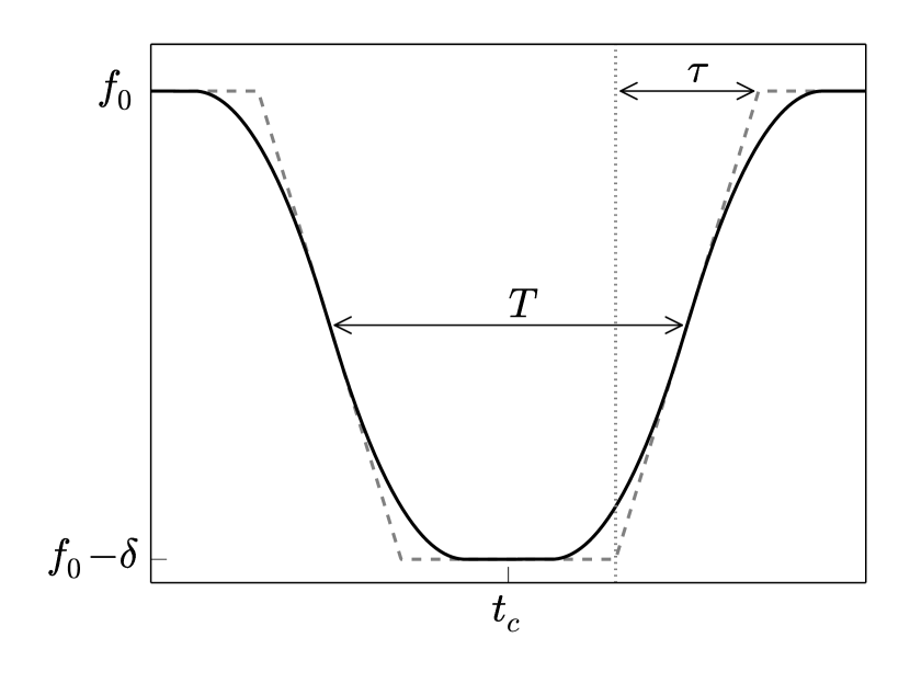
Following C08, we consider a simplified model for the light curve of a dark spherical planet of radius Rpsubscript𝑅𝑝R_{p} transiting in front of a spherical star of radius Rsubscript𝑅R_{*}. We neglect limb darkening and assume that the star has a uniform surface brightness f0subscript𝑓0f_{0}. We assume that the orbital period of the planet is long compared to the transit duration, so that the motion of the planet can be approximated by a constant velocity across the stellar disk. We then adopt the C08 light curve model that approximates the transit light curve as a piecewise linear function in time (Equation 1), where δ𝛿\delta is the transit depth, T𝑇T is the full-width half-max transit duration, and τ𝜏\tau is the ingress/egress duration, as shown in Figure 1; see Winn (2011) for a more complete description of these parameters.
Refer to caption
Figure 1.— Comparing the linear trapezoidal transit model (time vs. flux) of C08 (dashed, gray line) to the binned trapezoidal model of this work (solid, black line), for an illustrative set of parameters. For both models, T𝑇T is the full-width half-max duration of the transit event, τ𝜏\tau is the duration of ingress/egress, δ𝛿\delta is the transit depth, f0subscript𝑓0f_{0} is the out-of-transit flux level, and tcsubscript𝑡𝑐t_{c} is the time of transit center.
Fl(t;tc,δ,τ,T,f0)={f0δ,|ttc|T2τ2f0δ+δτ×(|ttc|T2+τ2),T2τ2<|ttc|<T2+τ2f0,|ttc|T2+τ2subscript𝐹𝑙𝑡subscript𝑡𝑐𝛿𝜏𝑇subscript𝑓0casessubscript𝑓0𝛿𝑡subscript𝑡𝑐𝑇2𝜏2missing-subexpressionsubscript𝑓0𝛿𝛿𝜏missing-subexpressionabsent𝑡subscript𝑡𝑐𝑇2𝜏2𝑇2𝜏2𝑡subscript𝑡𝑐𝑇2𝜏2subscript𝑓0𝑡subscript𝑡𝑐𝑇2𝜏2F_{l}\left(t;~{}t_{c},\delta,\tau,T,f_{0}\right)=\\ \begin{cases}f_{0}-\delta,&{}\left|t-t_{c}\right|\leq\frac{T}{2}-\frac{\tau}{2}\\ \!\begin{aligned} &f_{0}-\delta+\frac{\delta}{\tau}\\ &~{}\times\left(\left|t-t_{c}\right|-\frac{T}{2}+\frac{\tau}{2}\right),\end{aligned}&\frac{T}{2}-\frac{\tau}{2}<\left|t-t_{c}\right|<\frac{T}{2}+\frac{\tau}{2}\\ f_{0},&\left|t-t_{c}\right|\geq\frac{T}{2}+\frac{\tau}{2}\end{cases} (1)

As in C08, the parameters of the linear trapezoidal light curve model are related to the physical properties of the system (semi-major axis a𝑎a, inclination i𝑖i, eccentricity e𝑒e, longitude of periastron ω𝜔\omega, and mean motion n𝑛n) by,

δ𝛿\displaystyle\delta =\displaystyle= f0r2=f0(RpR)2subscript𝑓0superscript𝑟2subscript𝑓0superscriptsubscript𝑅𝑝subscript𝑅2\displaystyle f_{0}r^{2}=f_{0}\left(\frac{R_{p}}{R_{*}}\right)^{2} (2)
T𝑇\displaystyle T =\displaystyle= 2τ01b22subscript𝜏01superscript𝑏2\displaystyle 2\tau_{0}\sqrt{1-b^{2}} (3)
τ𝜏\displaystyle\tau =\displaystyle= 2τ0r1b2,2subscript𝜏0𝑟1superscript𝑏2\displaystyle 2\tau_{0}\frac{r}{\sqrt{1-b^{2}}}, (4)

where

b𝑏\displaystyle b \displaystyle\equiv acosiR(1e21+esinω)𝑎𝑖subscript𝑅1superscript𝑒21𝑒𝜔\displaystyle\frac{a\cos{i}}{R_{*}}\left(\frac{1-e^{2}}{1+e\sin\omega}\right) (5)
τ0subscript𝜏0\displaystyle\tau_{0} \displaystyle\equiv Ran(1e21+esinω).subscript𝑅𝑎𝑛1superscript𝑒21𝑒𝜔\displaystyle\frac{R_{*}}{an}\left(\frac{\sqrt{1-e^{2}}}{1+e\sin\omega}\right). (6)

Here, b𝑏b is the impact parameter, and τ0subscript𝜏0\tau_{0} is the timescale for the planet to move one stellar radius (projected on the sky).

We integrate the C08 linear transit light curve in time, to account for a finite integration time, \mathcal{I}. We denote by Flb(t)subscript𝐹𝑙𝑏𝑡F_{lb}(t) the average received flux (in the linear model) over a time interval \mathcal{I} centered on time t𝑡t. We restrict our consideration to scenarios with <Tτ𝑇𝜏\mathcal{I}<T-\tau, because otherwise the measurement of the transit depth during totality will be completely washed out by the integration time.

Flb(t;tc,δ,τ,T,f0,)={f0δ,if|ttc|T2τ22f0δ+δ2τ(|ttc|+2T2+τ2)2,ifT2τ22<|ttc|T2|τ22|f0δ+δmax(τ,)(|ttc|T2+max(τ,)2),ifT2|τ22|<|ttc|<T2+|τ22|f0δ2τ(T2+τ2+2|ttc|)2,ifT2+|τ22||ttc|<T2+τ2+2f0,if|ttc|T2+τ2+2subscript𝐹𝑙𝑏𝑡subscript𝑡𝑐𝛿𝜏𝑇subscript𝑓0casessubscript𝑓0𝛿if𝑡subscript𝑡𝑐𝑇2𝜏22f0δ+δ2τ(|ttc|+2T2+τ2)2,otherwiseotherwiseif𝑇2𝜏22𝑡subscript𝑡𝑐𝑇2𝜏22f0δ+δmax(τ,)(|ttc|T2+max(τ,)2),otherwiseotherwiseif𝑇2𝜏22𝑡subscript𝑡𝑐𝑇2𝜏22f0δ2τ(T2+τ2+2|ttc|)2,otherwiseotherwiseif𝑇2𝜏22𝑡subscript𝑡𝑐𝑇2𝜏22subscript𝑓0if𝑡subscript𝑡𝑐𝑇2𝜏22F_{lb}\left(t;~{}t_{c},\delta,\tau,T,f_{0},\mathcal{I}\right)=\\ \begin{cases}f_{0}-\delta,&\mathrm{if~{}}\left|t-t_{c}\right|\leq\frac{T}{2}-\frac{\tau}{2}-\frac{\mathcal{I}}{2}\\[5.0pt] \makebox[0.0pt][l]{$f_{0}-\delta+\frac{\delta}{2\tau\mathcal{I}}\left(\left|t-t_{c}\right|+\frac{\mathcal{I}}{2}-\frac{T}{2}+\frac{\tau}{2}\right)^{2}$,}\\[5.0pt] &\mathrm{if~{}}\frac{T}{2}-\frac{\tau}{2}-\frac{\mathcal{I}}{2}<\left|t-t_{c}\right|\leq{}\frac{T}{2}-\left|\frac{\tau}{2}-\frac{\mathcal{I}}{2}\right|\\[5.0pt] \makebox[0.0pt][l]{$f_{0}-\delta+\frac{\delta}{\max\left({\tau,\mathcal{I}}\right)}\left(\left|t-t_{c}\right|-\frac{T}{2}+\frac{\max\left({\tau,\mathcal{I}}\right)}{2}\right)$,}\\[5.0pt] &\mathrm{if~{}}\frac{T}{2}-\left|\frac{\tau}{2}-\frac{\mathcal{I}}{2}\right|<\left|t-t_{c}\right|<\frac{T}{2}+\left|\frac{\tau}{2}-\frac{\mathcal{I}}{2}\right|\\[5.0pt] \makebox[0.0pt][l]{$f_{0}-\frac{\delta}{2\tau\mathcal{I}}\left(\frac{T}{2}+\frac{\tau}{2}+\frac{\mathcal{I}}{2}-\left|t-t_{c}\right|\right)^{2}$,}\\[5.0pt] &\mathrm{if~{}}\frac{T}{2}+\left|\frac{\tau}{2}-\frac{\mathcal{I}}{2}\right|\leq\left|t-t_{c}\right|<\frac{T}{2}+\frac{\tau}{2}+\frac{\mathcal{I}}{2}\\[5.0pt] f_{0},&\mathrm{if~{}}\left|t-t_{c}\right|\geq\frac{T}{2}+\frac{\tau}{2}+\frac{\mathcal{I}}{2}\end{cases} (7)

Equation 7 gives the the binned light curve model for cases where <Tτ𝑇𝜏\mathcal{I}<T-\tau. Moving forward, we will differentiate between scenarios where the integration times less than the ingress/egress time, <τ𝜏\mathcal{I}<\tau (case 1), and and scenarios where >τ𝜏\mathcal{I}>\tau (case 2).

3. Fisher information analysis

When fitting a model to observed data, one is evaluating the likelihood of the observed data, {y}𝑦\{y\}, conditioned on a hypothesis, typically given in the form of a parametric model f({a})𝑓𝑎f(\{a\}). In this scenario, one is asking the question, “What is the probability of each of my data given the set of parameters {a}𝑎\{a\}?” In addition to seeking the parameters that maximize the likelihood of observing the data, one is often also interested in the sensitivity of the data to the model parameters, with the aim of placing confidence intervals on the “best-fitting” parameters. In this case one is asking, “What is the sensitivity of my data to small changes in the model parameters?”

The Fisher information formalism provides a means of addressing this question. The diagonal elements of the Fisher information matrix encode the variance of each parameter, and the off-diagonal elements give the covariances of the parameters. The magnitudes of the variances and covariances are a function of both the nature of the model and the uncertainties in the data.

In the special case that the observed data are normally, identically, and independently distributed about the model with constant total uncertainty σ𝜎\sigma, and assuming flat priors on each of the model parameters, the Fisher information matrix is simply the inverse of the covariance matrix that is often a byproduct of a traditional least-squares analysis. The full details of the Fisher information matrix derivation is given in Appendix A.

We apply Fisher information formalism to the integrated trapezoidal light curve model to derive two different sets of covariance matrices. First, we use the {tc,τ,T,δ,f0}subscript𝑡𝑐𝜏𝑇𝛿subscript𝑓0\{t_{c},\tau,T,\delta,f_{0}\} parametrization in both the τ>𝜏\tau>\mathcal{I} and τ<𝜏\tau<\mathcal{I} regimes; then, we transform these matrices to a second, more physical parametrization adopted by C08, {tc,b2,τ02,r,f0}subscript𝑡𝑐superscript𝑏2superscriptsubscript𝜏02𝑟subscript𝑓0\{t_{c},b^{2},\tau_{0}^{2},r,f_{0}\}. We consider this parameterization to be more physical because its parameters are more closely related to the properties of the system, and they are of more astronomical interest when characterizing planet systems.

All of the variances and covariances we derive in Appendix A are scaled by the common factor σ2/Γsuperscript𝜎2Γ\sigma^{2}/\Gamma, where ΓΓ\Gamma is the sampling rate of the light curve. Formally, the analysis assumes a single transit light curve sampled at rate ΓΓ\Gamma. For phase-folded data spanning several transits, we can let Ttot=Psubscript𝑇tot𝑃T_{\mathrm{tot}}=P, where Ttotsubscript𝑇totT_{\mathrm{tot}} is the length of the observation baseline and P𝑃P is the orbital period; then we may substitute an “effective” sampling rate, ΓeffsubscriptΓeff\Gamma_{\mathrm{eff}}, which can be at most NΓ𝑁ΓN\Gamma if N𝑁N transits were observed. Practically, we can define ΓeffsubscriptΓeff\Gamma_{\mathrm{eff}} as the reciprocal of the average time between consecutive phase-folded time points (see Section 7.3 for a discussion of the effects of phase sampling on ΓeffsubscriptΓeff\Gamma_{\mathrm{eff}}). ΓeffsubscriptΓeff\Gamma_{\mathrm{eff}} can be expressed independently of the integration time \mathcal{I} and can be substituted directly for ΓΓ\Gamma when appropriate. The Fisher information analysis assumes that the orbital period P𝑃P is known with absolute certainty when applied to phase-folded data, so the uncertainty on the transit midtime tcsubscript𝑡𝑐t_{c} is not representative of that for individual transits if ΓeffsubscriptΓeff\Gamma_{\mathrm{eff}} is used.

In some cases the out-of-transit flux level, f0subscript𝑓0f_{0}, is known to high enough precision that it can be fixed in the fitting process. In the following sections, we assume this is the case and look at the implications of Equations A8, A9, A15, and A16 for the precision of the transit parameters derived from fitting flux-normalized transits (f0=1)subscript𝑓01\left(f_{0}=1\right).

It turns out that, under the assumption of a multivariate normal distribution of the parameters, marginalizing over f0subscript𝑓0f_{0} is equivalent to removing the row and column that contain the variance of f0subscript𝑓0f_{0} and covariances of f0subscript𝑓0f_{0} with the other parameters and substituting the mean value of f0subscript𝑓0f_{0} (here assumed to be f0=1subscript𝑓01f_{0}=1) in the remaining matrix (e.g., Coe, 2009).

4. Numerical experiments

The covariance expressions (Equations A8, A9, A15, and A16) predict the uncertainties in the model parameters for a given dataset; we investigated their applicability with numerical experiments, in which we generated simulated transit photometry data and then fit the light curves to retrieve the transit parameters, uncertainties, and covariances.

We synthesized light curves by numerically integrating the C08 linear flux model over a 30-minute integration time, with time steps evenly spaced at 3-minute intervals. This choice corresponds to an effective sampling rate Γeff=10ΓsubscriptΓeff10Γ\Gamma_{\mathrm{eff}}=10\Gamma, with ΓΓ\Gamma the 30-minute Kepler long-cadence rate. We assumed that ten transits were measured at sampling rate ΓΓ\Gamma and then phase-folded over one orbital period (see Section 7.3 for a discussion on the effects of sampling rate and phase). We then added white noise using a pseudo-random number generator to the relative photometry at a level of σi=5×10⁵subscript𝜎𝑖5superscript105\sigma_{i}=5\times 10^{-5} per long-cadence sample.

To retrieve the variances (uncertainties) and covariances of the transit parameters, we fit a binned trapezoidal light curve model (Equation 7) to our simulated, phase-folded photometry. We used the known, “true” light curve parameters as a starting point to sample the joint four-dimensional likelihood distribution with emcee, an affine-invariant ensemble sampler for Markov chain Monte Carlo (MCMC) implemented in the Python programming language (Foreman-Mackey et al., 2013, proposed by Goodman & Weare 2010). The burn-in of the MCMC was sufficiently long that the starting parameters should not have impacted the resulting posteriors. Using 3×1043superscript1043\times 10^{4} MCMC chain samples, we estimated the covariance matrix with the Python numpy.cov method.

For our numerical experiments, we considered nominal planet-star parameters corresponding to a Solar-twin (R=Rsubscript𝑅subscript𝑅direct-productR_{\star}=R_{\odot}, M=Msubscript𝑀subscript𝑀direct-productM_{\star}=M_{\odot}) transited by a Jupiter-sized planet (Rp/R=0.1subscript𝑅𝑝subscript𝑅0.1R_{p}/R_{\star}=0.1) on an eccentric orbit (e=0.16𝑒0.16e=0.16) transiting at periastron (ω=π/2𝜔𝜋2\omega=\pi/2) with P=9.55days𝑃9.55daysP=9.55~{}\rm{days} at impact parameter b=0.2𝑏0.2b=0.2. We explored the effect of varying the parameters Rp/Rsubscript𝑅𝑝subscript𝑅R_{p}/R_{\star}, e𝑒e, b𝑏b, and P𝑃P in Figures 2 to 7. For the experiment varying P𝑃P only, we fixed the baseline of the observations to be 909090 days instead of assuming that ten transits were observed. Our analytic expressions for the variances and covariances of both the shape parameters and the physical parameters agree well with the results of the MCMC numerical experiments.

5. Results

One of the most important effects of a finite integration time is to increase the magnitudes of the covariances among the parameters derived from fitting a transit light curve. A finite integration time also increases the variances of both the shape and the physical parameters derived from a transit light curve. In some regimes (small Rp/Rsubscript𝑅𝑝subscript𝑅R_{p}/R_{\star}, short P𝑃P, and low signal-to-noise ratio, S/N) the variances on T𝑇T and τ𝜏\tau can increase by an order of magnitude (Figure 2). The scaling of the variances with Rp/Rsubscript𝑅𝑝subscript𝑅R_{p}/R_{\star} and P𝑃P is also affected. Finite integration time makes the scaling of the variances with Rp/Rsubscript𝑅𝑝subscript𝑅R_{p}/R_{\star} universally stronger, while the dependence on P𝑃P becomes more complicated than a simple power law relation; the orbital period of a planet influences whether it falls in the τ<𝜏\tau<\mathcal{I} or <τ𝜏\mathcal{I}<\tau regime, and the variance on τ𝜏\tau increases substantially once τ<𝜏\tau<\mathcal{I}.

The variance on the transit depth, δ𝛿\delta, which governs the precision with with which the planet-to-star radius ratio can be inferred, is not strongly affected by a finite integration time. Accounting for a finite integration time, the variance in δ𝛿\delta increases by a factor 1.14 (assuming the nominal orbit parameters described in the previous section). This corresponds to a factor 1.06 increase on the uncertainty in the transit depth for Kepler’s 30-minute long-cadence data compared to the 1-minute short-cadence data. The transit depth shows stronger correlations with T𝑇T (negative correlation) and τ𝜏\tau (positive correlation), especially in cases with low S/N.

The time of transit center is especially important for measuring transit timing variations (TTVs). The precision that can be obtained with the time of transit center tcsubscript𝑡𝑐t_{c} scales with the signal-to-noise of the transit detection in the light curve. From Equations A8 and A9,

σtc={1QτT2113ττ1QT211τ3>τ,subscript𝜎subscript𝑡𝑐cases1𝑄𝜏𝑇2113𝜏𝜏1𝑄𝑇211𝜏3𝜏\sigma_{t_{c}}=\left\{\begin{array}[]{lc}\frac{1}{Q}\sqrt{\frac{\tau T}{2}}\frac{1}{\sqrt{1-\frac{\mathcal{I}}{3\tau}}}&\tau\geq\mathcal{I}\\ \frac{1}{Q}\sqrt{\frac{\mathcal{I}T}{2}}\frac{1}{\sqrt{1-\frac{\tau}{3\mathcal{I}}}}&\mathcal{I}>\tau\end{array}\right.,

where Q=ΓTδσ𝑄Γ𝑇𝛿𝜎Q=\sqrt{\Gamma T}\frac{\delta}{\sigma} is the total signal-to-noise ratio of the transit in the limit r0𝑟0r\to 0. We note that for TTVs, tcsubscript𝑡𝑐t_{c} is measured for each individual transit; thus, the single transit sampling rate, ΓΓ\Gamma, should be used to predict σtcsubscript𝜎subscript𝑡𝑐\sigma_{t_{c}} for an individual transit, and not ΓeffsubscriptΓeff\Gamma_{\mathrm{eff}} for a phase-folded transit. From C08, the expected uncertainty in the transit time derived from an instantaneously sampled transit light curve is

lim0σtc=1QτT2.subscript0subscript𝜎subscript𝑡𝑐1𝑄𝜏𝑇2\lim_{\mathcal{I}\to 0}\sigma_{t_{c}}=\frac{1}{Q}\sqrt{\frac{\tau T}{2}}. (8)

A finite integration time introduces a /τ𝜏\mathcal{I}/\tau dependent correction factor, and effectively substitutes \mathcal{I} for τ𝜏\tau in the formula for σtcsubscript𝜎subscript𝑡𝑐\sigma_{t_{c}} in the >τ𝜏\mathcal{I}>\tau regime. Importantly, tcsubscript𝑡𝑐t_{c} remains uncorrelated with the other parameters when a finite integration time is taken into account.

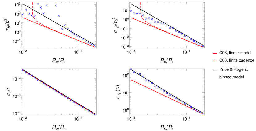
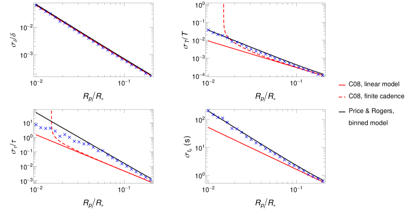
The dependence of variances and covariances of the light curve parameters on Rp/Rsubscript𝑅𝑝subscript𝑅R_{p}/R_{\star} are shown in Figures 2 and 3, respectively. The MCMC variances and covariances start to deviate from the analytic predictions once Rp/R<0.04subscript𝑅𝑝subscript𝑅0.04R_{p}/R_{\star}<0.04. This could be due to the fact that our integral approximation to the finite sums is breaking down at that point. Indeed, we see that Γeffτ<3subscriptΓeff𝜏3\Gamma_{\mathrm{eff}}\;\tau<3 for those small planet radii (see Section 7.3). Another possibility is that the posterior distribution of τ𝜏\tau is no longer Gaussian at this point (see Section 7.4).

In Figure 4, we plot the predicted and measured uncertainties of the “physical” parameters r𝑟r, b2superscript𝑏2b^{2}, and τ02superscriptsubscript𝜏02\tau_{0}^{2}. The deviation of the relative uncertainty in τ02superscriptsubscript𝜏02\tau_{0}^{2} at Rp/R<0.04subscript𝑅𝑝subscript𝑅0.04R_{p}/R_{\star}<0.04 seems to be caused by the corresponding deviation of the relative uncertainty of τ𝜏\tau. We note a significant deviation in the measured σb2subscript𝜎superscript𝑏2\sigma_{b^{2}}, but it does not have such an obvious explanation. Our results illustrate that b2superscript𝑏2b^{2} is the most difficult of the physical parameters to constrain, particularly at small Rp/Rsubscript𝑅𝑝subscript𝑅R_{p}/R_{\star}. As an additional test, by sampling from these parameters, instead of the trapezoidal parameters, in an MCMC fit to synthetic light curve data, we verified that the variances and covariances of the physical parameters obtained from fitting are consistent with these results.

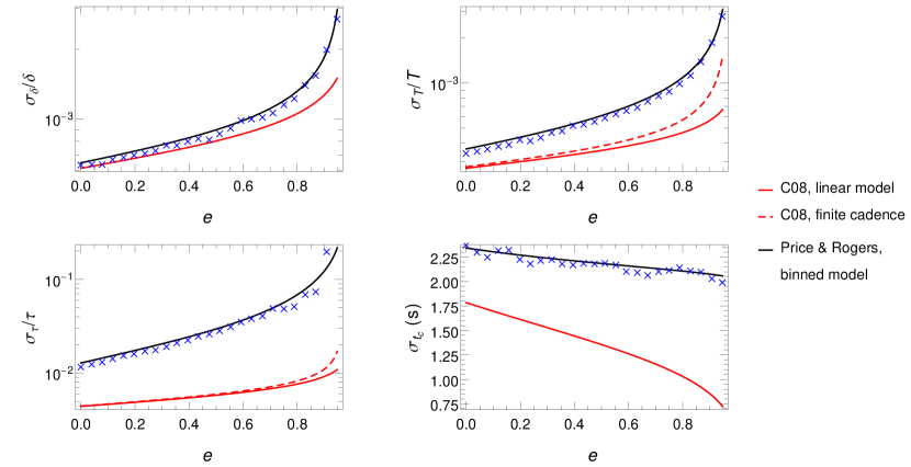
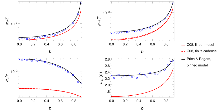
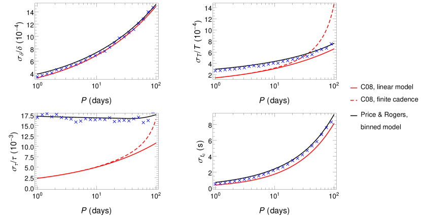
Figures 5, 6, and 7 show the predicted and measured uncertainties of the trapezoidal light curve parameters as functions of eccentricity e𝑒e, impact parameter b𝑏b, and orbital period P𝑃P, respectively. Our MCMC measured uncertainties appear to agree with the predictions in all cases, even at large values of e𝑒e and b𝑏b (see Section 7.1 for a discussion of the effects of grazing transits on our approximations). At large e𝑒e, the relative uncertainty in τ𝜏\tau increases by more than an order of magnitude from the C08 prediction, highlighting the importance of accounting for finite integration in such cases. Similarly, for small P𝑃P, the relative uncertainty on τ𝜏\tau increases significantly compared to previous predictions.

Our analytic expressions for the covariances and variances clearly agree better with the results from the simulated Kepler long cadence data than the finite cadence corrections from C08. The finite cadence corrections from C08 do not account for the averaging of the planet light curve over a finite integration time. In some cases where finite cadence corrections come to bear (e.g. in the variances of T𝑇T and τ𝜏\tau as Rp/Rsubscript𝑅𝑝subscript𝑅R_{p}/R_{\star} gets smaller), finite integration time may actually improve the variances of T𝑇T and τ𝜏\tau compared to the predictions of C08 Equation 26. With finite integration time information on the ingress and egress is spread over any long exposure spanning the ingress and egress. In contrast, if the light curve is instantaneously sampled at the same cadence, the ingress and egress may be completely missed.
Refer to caption
Figure 2.— Relative uncertainties of the trapezoidal transit parameters derived from Kepler long-cadence data, as a function of Rp/Rsubscript𝑅𝑝subscript𝑅R_{p}/R_{\star}. The fiducial planet and star properties assumed are: R=Rsubscript𝑅subscript𝑅direct-productR_{\star}=R_{\odot}, M=Msubscript𝑀subscript𝑀direct-productM_{\star}=M_{\odot}, e=0.16𝑒0.16e=0.16, P=9.55days𝑃9.55daysP=9.55~{}\rm{days}, and b=0.2𝑏0.2b=0.2. The solid red line gives Rp/Rsubscript𝑅𝑝subscript𝑅R_{p}/R_{\star}, corresponding to the analytic predictions from Carter et al. (2008) (their Equation 20), the dashed red curve gives the analytic predictions from Carter et al. (2008) including a finite-cadence correction (their Equation 26), and the solid black curve presents the analytic predictions accounting for a finite integration time from this work (Equations A8 and A9). The uncertainties derived from an MCMC analysis of simulated long-cadence Kepler data (blue crosses) agree well with the predictions of this work; we plot the measured uncertainty scaled by the true value of the parameter (where appropriate), so this plot does not reflect any systematic error in parameter measurement.
Refer to caption
Figure 3.— Covariances in the trapezoidal approximation transit parameters derived from simulated Kepler long-cadence data, as a function of Rp/Rsubscript𝑅𝑝subscript𝑅R_{p}/R_{\star}, corresponding to the same scenarios presented in Figure 2.
Refer to caption
Figure 4.— Relative uncertainties in the physical transit parameters derived from simulated Kepler long-cadence data, as a function of Rp/Rsubscript𝑅𝑝subscript𝑅R_{p}/R_{\star}, corresponding to the same scenarios presented in Figure 2. We scale by the true value of the parameter to isolate the uncertainty from systematic error in parameter measurement.
Refer to caption
Figure 5.— Relative uncertainties of the trapezoidal transit parameters derived from Kepler long-cadence data, as functions of eccentricity e𝑒e. We have assumed nominal planet parameters R=Rsubscript𝑅subscript𝑅direct-productR_{\star}=R_{\odot}, M=Msubscript𝑀subscript𝑀direct-productM_{\star}=M_{\odot}, P=9.55days𝑃9.55daysP=9.55~{}\text{days}, b=0.2𝑏0.2b=0.2, and r=0.1𝑟0.1r=0.1. To isolate systematic error in parameter measurement from parameter uncertainty, the relative uncertainties are scaled by the true value of the parameter.
Refer to caption
Figure 6.— Relative uncertainties of the trapezoidal transit parameters derived from Kepler long-cadence data, as functions of impact parameter b𝑏b. We have assumed nominal planet parameters R=Rsubscript𝑅subscript𝑅direct-productR_{\star}=R_{\odot}, M=Msubscript𝑀subscript𝑀direct-productM_{\star}=M_{\odot}, P=9.55days𝑃9.55daysP=9.55~{}\text{days}, e=0.16𝑒0.16e=0.16, and r=0.1𝑟0.1r=0.1. To isolate systematic error in parameter measurement from parameter uncertainty, the relative uncertainties are scaled by the true value of the parameter.
Refer to caption
Figure 7.— Relative uncertainties of the trapezoidal transit parameters derived from Kepler long-cadence data, as functions of impact parameter P𝑃P; for this experiment only, we fix the baseline of the observations to be 909090 days, instead of assuming that ten transits were observed. We have assumed nominal planet parameters R=Rsubscript𝑅subscript𝑅direct-productR_{\star}=R_{\odot}, M=Msubscript𝑀subscript𝑀direct-productM_{\star}=M_{\odot}, b=0.2𝑏0.2b=0.2, e=0.16𝑒0.16e=0.16, and r=0.1𝑟0.1r=0.1. To isolate systematic error in parameter measurement from parameter uncertainty, the relative uncertainties are scaled by the true value of the parameter.

6. Survey planning

There are several space- and ground-based transit surveys on the horizon, including TESS, K2, and PLATO. Equations A8, A9, A15 and A16 can be used to help choose an optimal integration time for photometric surveys for transiting planets when combined with models for the frame rate and photometric measurement uncertainty of the particular instrument.

In the Equations A8, A9, A15 and A16, the photometric precision σ𝜎\sigma and integration time \mathcal{I} are separate parameters. In practice, the uncertainty on a given photometric point will depend on the integration time chosen. For photon-noise, σ/f01/2proportional-to𝜎subscript𝑓0superscript12\sigma/f_{0}\propto\mathcal{I}^{-1/2}. We have kept our equations explicitly in terms of σ𝜎\sigma (instead of directly substituting in the assumption of photon-noise) so that they can be more flexibly applied to cases where additional white noise sources add to the photometric measurement uncertainty.

The integration time also affects the effective phase sampling of the light curve. For continuous photometric observations over a time baseline, Ttotsubscript𝑇totT_{\mathrm{tot}}, the effective sampling of the phase-folded light curve can be up to

Γeff=TtotP(+tread).subscriptΓeffsubscript𝑇tot𝑃subscript𝑡read\Gamma_{\mathrm{eff}}=\frac{T_{\mathrm{tot}}}{P\left(\mathcal{I}+t_{\mathrm{read}}\right)}. (9)

We denote by treadsubscript𝑡readt_{\mathrm{read}} the time needed for the photometer to read out; (+tread)1superscriptsubscript𝑡read1\left(\mathcal{I}+t_{\mathrm{read}}\right)^{-1} is the CCD frame rate. The factor Ttot/Psubscript𝑇tot𝑃T_{\mathrm{tot}}/P accounts for the number of transits detected over the span of the observations. This maximal effective sampling rate is achieved in the case where there is no clustering of photometric points at specific orbital phases.

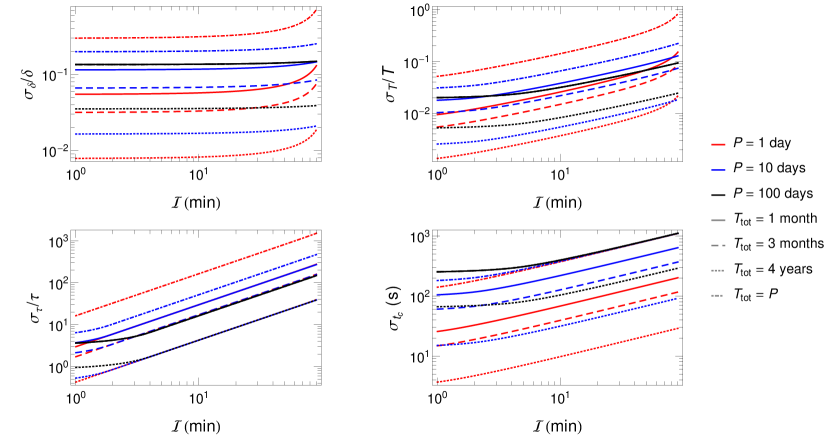
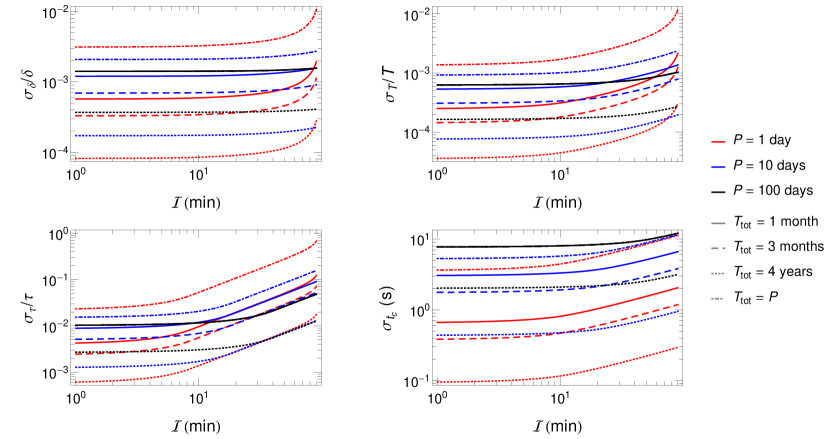
In the case of a photon-noise limited survey with negligible read out time (tread=0)subscript𝑡read0\left(t_{\mathrm{read}}=0\right), the \mathcal{I} dependence cancels in the σ2/Γeffsuperscript𝜎2subscriptΓeff\sigma^{2}/\Gamma_{\mathrm{eff}} prefactor that scales all the covariance matrices. In these limits, the integration time dependence comes solely from the body of the covariance matrix elements in Equations A8, A9, A15 and A16. We plot in Figure 8 how the uncertainties on the transit parameters predicted for a Jupiter transiting a Sun-twin in a photon-noise limited survey with negligible read-out time depend on \mathcal{I}, Ttotsubscript𝑇totT_{\mathrm{tot}}, and P𝑃P. We assumed a nominal photometric precision of σ/f0=5×105𝜎subscript𝑓05superscript105\sigma/f_{0}=5\times 10^{-5} for a 30 minute exposure; choosing a different value for σ𝜎\sigma would simply amount to rescaling the vertical axis on the figure. In Figure 9, we make the same plot for a 1R1subscript𝑅direct-sum1~{}R_{\oplus} planet orbiting a Sun-twin, assuming the same nominal orbit parameters.

Lower integration times mean better precision, but after a certain point there is a plateau regime in which shorter integration times do not improve the relative precision of the transit parameters derived from the light curve (see Figures 8 and 9). In planning a transit survey, choosing an integration time near the “knee” would be optimal to minimize both the data rate and the relative uncertainties on the derived planet properties. The critical integration time depends on both the planet orbital period and Rp/Rsubscript𝑅𝑝subscript𝑅R_{p}/R_{*}, but is not significantly affected by the survey duration, Ttotsubscript𝑇totT_{\mathrm{tot}}. Planets with shorter P𝑃P and smaller Rp/Rsubscript𝑅𝑝subscript𝑅R_{p}/R_{*} have smaller critical integration times, and their characterization would benefit more greatly from short cadence observations.

The critical integration time delimiting the beginning of the plateau regime is different for different transit parameters of interest. The critical integration time for τ𝜏\tau is the shortest. In planning a survey, one would want to consider the smallest critical integration time among the parameters of interest. Exposure times of 3, 10, and 30 minutes are optimal for sampling the transits of Jupiter-sized planets orbiting Sun twins on 1-day, 10-day, and 100-day orbits, respectively (Figure 8). In contrast, for Earth-sized planets with Rp/R=102subscript𝑅𝑝subscript𝑅superscript102R_{p}/R_{*}=10^{-2} the plateau in the relative uncertainty in τ𝜏\tau occurs at <1minute1minute\mathcal{I}<1~{}\rm{minute} (Figure 9), regardless of the orbital period.
Refer to caption
Figure 8.— Uncertainties of trapezoidal transit parameters for representative observing cases as functions of integration time \mathcal{I}, as predicted by the binned trapezoidal light curve model, for Jupiter-size planets orbiting Sun twins. We show cases for orbits of 1 day (red curves), 10 days (blue curves), and 100 days (black curves) and total survey lengths of 1 month (TESS-like; solid curves), 3 months (dashed curves), 4 years (Kepler-like; dotted curves), and one orbital period (dot-dashed curves). We assume nominal parameter values b=0.2𝑏0.2b=0.2, e=0.16𝑒0.16e=0.16, and r=0.1𝑟0.1r=0.1, to remain consistent with the figures above; we scale the photometric uncertainty such that a Kepler 30-minute exposure corresponds to σ=5×10⁵𝜎5superscript105\sigma=5\times 10^{-5}, and we assume photon-noise is the only noise source. ΓeffsubscriptΓeff\Gamma_{\mathrm{eff}} is given by Equation 9 when Ttot>Psubscript𝑇tot𝑃T_{\mathrm{tot}}>P; otherwise, Γeff=1/subscriptΓeff1\Gamma_{\mathrm{eff}}=1/\mathcal{I}. The special case Ttot=Psubscript𝑇tot𝑃T_{\mathrm{tot}}=P corresponds to the precision on the parameters derived from fitting a single transit light curve.
Refer to caption
Figure 9.— Uncertainties of trapezoidal transit parameters for representative observing cases as functions of integration time \mathcal{I}, as predicted by the binned trapezoidal light curve model, for Earth-size planets orbiting Sun twins. We show cases for orbits of 1 day, 10 days, and 100 days and total survey lengths of 1 month, 3 months, 4 years, and one orbital period. We assume nominal parameter values b=0.2𝑏0.2b=0.2, e=0.16𝑒0.16e=0.16, and r=0.01𝑟0.01r=0.01 and scale the photometric uncertainty such that a Kepler 30-minute exposure corresponds to σ=5×10⁵𝜎5superscript105\sigma=5\times 10^{-5}, and we assume photon-noise is the only noise source. ΓeffsubscriptΓeff\Gamma_{\mathrm{eff}} is given by Equation 9 when Ttot>Psubscript𝑇tot𝑃T_{\mathrm{tot}}>P; otherwise, Γeff=1/subscriptΓeff1\Gamma_{\mathrm{eff}}=1/\mathcal{I}. The line styles and colors are identical to those in Figure 8.

7. Discussion

In this section we revisit some of the approximations involved in deriving our covariance matrices, exploring their effects and quantifying the limitations they impose on the applicability of Equations A8, A9, A15, and A16.

7.1. Effect of grazing transits

We have thus far limited our discussion to cases in which the integration time does not exceed the time between second and third contact, when the planet disk is contained completely within the disk of the star. Once the integration time exceeds Tτ𝑇𝜏T-\tau, the maximum apparent depth of the transit light curve starts to decrease as all exposures taken during totality are diluted by flux during ingress, egress, and/or out-of-transit. The apparent maximum depth of the transit light curve can be reduced by as much as T/𝑇T/\mathcal{I}; this maximum value corresponds to >T+τ𝑇𝜏\mathcal{I}>T+\tau.

By focusing on cases with <Tτ𝑇𝜏\mathcal{I}<T-\tau, we are effectively limiting the range of orbital inclinations (or impact parameters, b𝑏b) considered. We are neglecting grazing transits, with impact parameters b𝑏b in excess of a maximum value, bmaxsubscript𝑏𝑚𝑎𝑥b_{max}, given by combining Equations 3 and 4,

bmax=[1r(1+x22r+(x22r)(x22r+2))]1/2,subscript𝑏𝑚𝑎𝑥superscriptdelimited-[]1𝑟1superscript𝑥22𝑟superscript𝑥22𝑟superscript𝑥22𝑟212b_{max}=\left[1-r\left(1+\frac{x^{2}}{2r}+\sqrt{\left(\frac{x^{2}}{2r}\right)\left(\frac{x^{2}}{2r}+2\right)}\right)\right]^{1/2}, (10)

where x=2τ0𝑥2subscript𝜏0x=\frac{\mathcal{I}}{2\tau_{0}}. In the case of long orbital periods (x22rmuch-less-thansuperscript𝑥22𝑟x^{2}\ll 2r) bmaxsubscript𝑏𝑚𝑎𝑥b_{max} approaches 1r1𝑟1-r, the limiting value for the disk of the planet to be circumscribed by the stellar disk. For shorter periods (10less-than-or-similar-toabsent10\lesssim 10 days) the constraints on b𝑏b for which our results apply can be significantly more restrictive (Figure 10). Limb-darkening could have an important effect on these grazing transits, and may lead to the breakdown of the C08 trapezoidal light curve approximations anyway, in the excluded regime of b>bmax𝑏subscript𝑏𝑚𝑎𝑥b>b_{max}.

Though we have not provided analytic equations for the covariance matrix in the case where >Tτ𝑇𝜏\mathcal{I}>T-\tau, these can be readily derived following a similar approach as in Appendix A, below. There are in fact, three more regimes to be considered (in addition to cases 1 and 2 given in Equation 7): Tτ<<T+τ𝑇𝜏𝑇𝜏T-\tau<\mathcal{I}<T+\tau and <τ𝜏\mathcal{I}<\tau (case 3); Tτ<<T+τ𝑇𝜏𝑇𝜏T-\tau<\mathcal{I}<T+\tau and >τ𝜏\mathcal{I}>\tau (case 4); and >T+τ𝑇𝜏\mathcal{I}>T+\tau (case 5).

Refer to caption
Figure 10.— Maximum impact parameter, bmaxsubscript𝑏𝑚𝑎𝑥b_{max}, as a function of orbital period for Jupiter-sized (r=0.1𝑟0.1r=0.1, solid line) and Earth-sized (r=0.01𝑟0.01r=0.01, dashed) planets on circular orbits around a Sun-twin star with Kepler long-cadence sampling (=30minutes30minutes\mathcal{I}=30~{}\rm{minutes}).

7.2. Effect of limb darkening

So far, we have neglected the effect of limb-darkening (following C08), and have considered a planet transiting a star with uniform surface brightness. To explore the effects of limb darkening, we generated synthetic transit data with a Python implementation of the Eastman et al. (2013) EXOFAST occultquad routine, which generates a Mandel & Agol (2002) quadratically limb-darkened light curve. We chose the limb darkening parameters for HAT-P-2 as our test case, obtaining the parameters with the Eastman et al. (2013) limb darkening parameter applet111http://astroutils.astronomy.ohio-state.edu/exofast/limbdark.shtml, which interpolates the Claret & Bloemen (2011) quadratic limb darkening tables.

We fit each synthetic data set with three different models (the trapezoidal model described in this paper, a Mandel & Agol model with fixed limb darkening parameters, or a Mandel & Agol model with limb darkening coefficients as free parameters). We used a procedure similar to that described in Section 4 but with 1.5×1051.5superscript1051.5\times 10^{5} samples. To minimize the covariances between model parameters, we parametrized all models in terms of δ𝛿\delta, T𝑇T, τ𝜏\tau, and tcsubscript𝑡𝑐t_{c}. The limb darkened model also included the Kipping (2013) limb darkening parameters q1subscript𝑞1q_{1} and q2subscript𝑞2q_{2}, which map directly to the quadratic coefficients u1subscript𝑢1u_{1} and u2subscript𝑢2u_{2}, as free parameters. Since fitting eccentricity e𝑒e and argument of periastron ω𝜔\omega is difficult and computationally intensive, we have restricted this test to e=0𝑒0e=0 cases only.

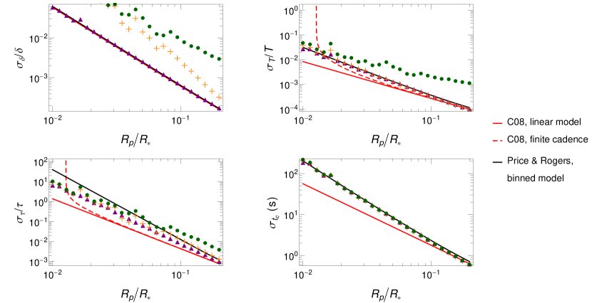
We show the results of this analysis in Figures 11 and 12. In the case of the trapezoidal model, our Equations A8, A9, A15, and A16 do well to predict the uncertainties on δ𝛿\delta, T𝑇T, and tcsubscript𝑡𝑐t_{c}, but we overpredict the uncertainty in τ𝜏\tau. T𝑇T becomes more correlated with δ𝛿\delta and with τ𝜏\tau when limb darkening is taken into account. When the synthetic data are fit with a Mandel & Agol model with fixed limb darkening, the uncertainty in the transit depth δ𝛿\delta increases. Our predictions apply well to T𝑇T and tcsubscript𝑡𝑐t_{c} in this case, while the uncertainty in τ𝜏\tau is still overpredicted. Finally, when limb darkening coefficients are added as free parameters, the uncertainty in δ𝛿\delta increases further, and we underpredict the uncertainty in T𝑇T significantly, as expected. To accurately predict the uncertainties in this case, q1subscript𝑞1q_{1} and q2subscript𝑞2q_{2} should be included as parameters in the Fisher information analysis. The uncertainty in τ𝜏\tau is overpredicted in the small Rp/Rsubscript𝑅𝑝subscript𝑅R_{p}/R_{\star} regime and underpredicted in the large Rp/Rsubscript𝑅𝑝subscript𝑅R_{p}/R_{\star} regime. When a Mandel & Agol model is used, we find that our equations are not as useful for predicting the parameter covariances.
Refer to caption
Figure 11.— Relative uncertainties of the trapezoidal transit parameters for a Mandel & Agol (2002) quadratically limb darkened light curve, integrated with =30minutes30minutes\mathcal{I}=30~{}\text{minutes}, as a function of Rp/Rsubscript𝑅𝑝subscript𝑅R_{p}/R_{\star}. The uncertainties were measured with an MCMC analysis, with the relative uncertainties being scaled by the true value of the parameter. We fit synthetic light curves with the trapezoidal model described in this paper (purple triangles), a Mandel & Agol model with fixed limb darkening parameters (orange crosses), and a Mandel & Agol model with limb darkening coefficients as free parameters (green points). Our predictions (solid black lines) are applicable for the trapezoidal model, though the uncertainty in τ𝜏\tau is overpredicted. The uncertainty in δ𝛿\delta increases when limb darkening is taken into account. The C08 prediction (solid red line) and finite cadence prediction (dashed red line) are shown for comparison. We let R=Rsubscript𝑅subscript𝑅direct-productR_{\star}=R_{\odot}, M=Msubscript𝑀subscript𝑀direct-productM_{\star}=M_{\odot}, e=0𝑒0e=0, P=9.55days𝑃9.55daysP=9.55~{}\text{days}, and b=0.2𝑏0.2b=0.2. As before, the uncertainties are scaled by the true value of the parameter, so systematic offsets are not reflected in this plot.
Refer to caption
Figure 12.— Covariances in the trapezoidal approximation transit parameters derived from simulated Kepler long-cadence data, as a function of Rp/Rsubscript𝑅𝑝subscript𝑅R_{p}/R_{\star}, corresponding to the same scenarios presented in Figure 11. Fitting with a binned trapezoidal model yields values of T𝑇T that are significantly more correlated with δ𝛿\delta and τ𝜏\tau than we predict at smaller values of Rp/Rsubscript𝑅𝑝subscript𝑅R_{p}/R_{*}. Our predictions are much less useful for predicting the parameter covariances of the Mandel & Agol models.

7.3. Effect of finite phase sampling

Our analysis makes the approximation that the data is sampled at a uniform rate. The ΓeffsubscriptΓeff\Gamma_{\mathrm{eff}} that we have defined for phase-folded data (Equation 9) is the maximum possible sampling rate for a continuous photometric time series. The approximation of a constant effective sampling rate for phase-folded data may break down if the planet orbital period is an integer (or rational number) multiple of the sampling cadence. In these scenarios, the photometric observations of different transits cluster at specific phases within the planet orbit and transit light curve, and the equal weighting of different phases in Equation A5 is no longer fully valid. This will produce scatter about our analytic expressions for the covariance matrix in the idealized sampling scenario.

Another obstacle to applying our variance and covariance approximations arises if too few transits have been observed to sufficiently cover the full range of planet phases during transit. In these cases, the integral approximation of equation A4 breaks down and the finite sums (Equation A3) must be evaluated numerically.

7.4. Effect of non-Gaussian posteriors

The posterior distribution of the trapezoidal parameters obtained from our MCMC fits to simulated Kepler long-cadence light curves are well approximated by Gaussians in high S/N scenarios. In cases of low S/N, however, the “normally-distributed parameters” assumption upon which the Fisher information matrix analysis relies can break down. The ingress/egress duration is physically constrained to be τ>0𝜏0\tau>0. When the uncertainty στsubscript𝜎𝜏\sigma_{\tau} becomes comparable to the magnitude of τ𝜏\tau itself, the truncation at τ=0𝜏0\tau=0 induces non-Gaussian posteriors. This may account for some of the deviations at small Rp/Rsubscript𝑅𝑝subscript𝑅R_{p}/R_{\star} in Figures 2 and 3. Solving numerically for the value of Rp/Rsubscript𝑅𝑝subscript𝑅R_{p}/R_{\star} where the value of τ𝜏\tau becomes comparable to στsubscript𝜎𝜏\sigma_{\tau} for nominal values of the other parameters, we find that τ𝜏\tau is equal to 3στ3subscript𝜎𝜏3\sigma_{\tau} at Rp/R0.042subscript𝑅𝑝subscript𝑅0.042R_{p}/R_{\star}\approx 0.042; it is equal to 2στ2subscript𝜎𝜏2\sigma_{\tau} when Rp/R0.037subscript𝑅𝑝subscript𝑅0.037R_{p}/R_{\star}\approx 0.037 and 1στ1subscript𝜎𝜏1\sigma_{\tau} when Rp/R0.031subscript𝑅𝑝subscript𝑅0.031R_{p}/R_{\star}\approx 0.031. As Rp/R0subscript𝑅𝑝subscript𝑅0R_{p}/R_{\star}\rightarrow 0, we expect the posterior to approach a Gaussian centered at 00 and truncated at 00; τ=3στ𝜏3subscript𝜎𝜏\tau=3\sigma_{\tau} is the approximate lower limit of τ𝜏\tau down to which truncation should not be apparent in the posterior distribution. The numerical results seem to coincide well with the value of Rp/Rsubscript𝑅𝑝subscript𝑅R_{p}/R_{\star} where the MCMC results begin to deviate from the analytic predictions.

7.5. Effect of other noise sources

Throughout this work, we have neglected the effects of correlated (red) noise on the light curve parameter uncertainties. For light curve data with significant red noise, we expect that our formulae will be less applicable, since we assume completely uncorrelated errors in the Fisher information analysis.

We have also neglected the effects of read noise σreadsubscript𝜎read\sigma_{\mathrm{read}}, noise that is intrinsic to the detector. Read noise adds in quadrature with photon-noise, thereby setting a minimum value of the overall uncertainty on each data point in the light curve. For shorter integration times \mathcal{I} and fainter stars, read noise may dominate the overall noise σ𝜎\sigma. In the σσread𝜎subscript𝜎read\sigma\to\sigma_{\mathrm{read}} limit, σconstantsimilar-to𝜎constant\sigma\sim\mathrm{constant}, Γeff1/similar-tosubscriptΓeff1\Gamma_{\mathrm{eff}}\sim 1/\mathcal{I}, and f0similar-tosubscript𝑓0f_{0}\sim\mathcal{I}, so all of the covariance elements we derive in Appendix A will be scaled by (σ/f0)2/Γeff1/similar-tosuperscript𝜎subscript𝑓02subscriptΓeff1\left(\sigma/f_{0}\right)^{2}/\Gamma_{\mathrm{eff}}\sim 1/\mathcal{I}. Thus, in the read-noise dominated regime, the uncertainties on transit parameters are expected to increase with shorter exposure times. In practice, the optimal integration time for a given target (assuming white noise) will be either the integration time at which read noise becomes the dominant noise source or the critical integration time assuming photon noise (the “knee” in Figures 8 and 9), whichever is longer.

8. Conclusions

Kipping (2010) highlighted the necessity of fitting a binned light curve model to binned light curve data. We have updated the Carter et al. (2008) analytic expressions for the variances and covariances of parameters derived from fitting transit light curve data, to take finite integration time into account.

With finite integration time, the uncertainties on the transit parameters are strictly greater than what one could extract from an instantaneously sampled light curve. The magnitude of the correlations among transit ingress/egress duration, transit duration and transit depth all increase, while the mid-transit time (relevant for measuring TTVs) remains uncorrelated. For example, for a Hot Jupiter or close-in Earth-size planet on a three day orbit the variances on δ𝛿\delta, tcsubscript𝑡𝑐t_{c}, τ𝜏\tau, and T𝑇T are 1.21.21.2, 2.52.52.5, 242424, and 2.82.82.8 times larger for 30-minute long-cadence data as compared to 1 minute short cadence data, assuming the nominal orbit parameters we have used throughout this work; the covariances can increase by as much as a factor of 303030. In contrast, for a transiting Earth-twin on a 1-year orbit, the variances themselves are larger in magnitude, but they do not change greatly with integration time.

We provide Python and Mathematica code for computing the predicted variances and covariances that could be measured using the binned light curve model. Phasing, red noise, non-Gaussianities, and other effects can affect the actual uncertainties obtained from a full analysis. Our analytic expressions are still helpful for target selection, observation planning, and rule of thumb intuition. Today, finite integration time is relevant for Kepler long-cadence light curves, and will remain important in the future analysis of data from K2 and from TESS full frame images.

9. Acknowledgements

We would like to thank John Johnson of the Harvard-Smithsonian Center for Astrophysics for his valuable input on this project and for establishing the Johnson Exolab as an environment where undergraduates and postdoctoral scholars can work together on projects like this one. We would also like to thank the referee for providing a very helpful and constructive review of this work. EMP acknowledges funding provided by Mr. and Mrs. Carl Larson for her 2013 Carolyn Ash SURF Fellowship. LAR acknowledges support provided by NASA through Hubble Fellowship grant #HF-51313.01 awarded by the Space Telescope Science Institute, which is operated by the Association of Universities for Research in Astronomy, Inc., for NASA, under contract NAS 5-26555. The LevelScheme (Caprio, 2005) scientific figure preparation system for Mathematica was used in the preparation of this paper.

Appendix A Full derivation of Fisher information and covariance matrices

For N𝑁N data points {y}𝑦\{y\} and model points {ymod}subscript𝑦mod\{y_{\rm mod}\} which depend on a set of parameters {p}𝑝\{p\}, and under the assumption of uncorrelated errors of constant absolute magnitude σ𝜎\sigma, we begin with the likelihood function (see e.g., Gould, 2003)

=1σ2πexp[12σ2k=1N(ykyk,mod)2].1𝜎2𝜋12superscript𝜎2superscriptsubscript𝑘1𝑁superscriptsubscript𝑦𝑘subscript𝑦𝑘mod2\mathcal{L}=\frac{1}{\sigma\sqrt{2\pi}}\exp{\left[-\frac{1}{2}\sigma^{-2}\sum\limits_{k=1}^{N}\left(y_{k}-y_{k,\text{mod}}\right)^{2}\right]}. (A1)

The Fisher information matrix 𝐁𝐁\mathbf{B} is defined by (see e.g., Vallisneri, 2008),

Bijsubscript𝐵𝑖𝑗\displaystyle B_{ij} =(pilog)(pjlog)absentdelimited-⟨⟩subscript𝑝𝑖subscript𝑝𝑗\displaystyle=\langle\left(\frac{\partial}{\partial p_{i}}\log{\mathcal{L}}\right)\left(\frac{\partial}{\partial p_{j}}\log{\mathcal{L}}\right)\rangle
=(σ4k=1Nl=1N(ykyk,mod)(ylyl,mod)yk,modpiyl,modpj)absentdelimited-⟨⟩superscript𝜎4superscriptsubscript𝑘1𝑁superscriptsubscript𝑙1𝑁subscript𝑦𝑘subscript𝑦𝑘modsubscript𝑦𝑙subscript𝑦𝑙modsubscript𝑦𝑘modsubscript𝑝𝑖subscript𝑦𝑙modsubscript𝑝𝑗\displaystyle=\langle\left(\sigma^{-4}\sum\limits_{k=1}^{N}\sum\limits_{l=1}^{N}\left(y_{k}-y_{k,\text{mod}}\right)\left(y_{l}-y_{l,\text{mod}}\right)\frac{\partial y_{k,\text{mod}}}{\partial p_{i}}\frac{\partial y_{l,\text{mod}}}{\partial p_{j}}\right)\rangle
=σ2k=1N(yk,modpi)(yk,modpj)absentsuperscript𝜎2superscriptsubscript𝑘1𝑁subscript𝑦𝑘modsubscript𝑝𝑖subscript𝑦𝑘modsubscript𝑝𝑗\displaystyle=\sigma^{-2}\sum\limits_{k=1}^{N}\left(\frac{\partial y_{k,\text{mod}}}{\partial p_{i}}\right)\left(\frac{\partial y_{k,\text{mod}}}{\partial p_{j}}\right) (A2)

where xdelimited-⟨⟩𝑥\langle x\rangle denotes the expected value of x𝑥x. For our application to transit light curves, the model function is ymod=Flbsubscript𝑦𝑚𝑜𝑑subscript𝐹𝑙𝑏y_{mod}=F_{lb} and p={tc,τ,T,δ,f0}𝑝subscript𝑡𝑐𝜏𝑇𝛿subscript𝑓0p=\{t_{c},\tau,T,\delta,f_{0}\}, so

Bij=σ2k=1N[piFlb(tk;{p})][pjFlb(tk;{p})].subscript𝐵𝑖𝑗superscript𝜎2superscriptsubscript𝑘1𝑁delimited-[]subscript𝑝𝑖subscript𝐹𝑙𝑏subscript𝑡𝑘𝑝delimited-[]subscript𝑝𝑗subscript𝐹𝑙𝑏subscript𝑡𝑘𝑝B_{ij}=\sigma^{-2}\sum\limits_{k=1}^{N}\left[\frac{\partial}{\partial p_{i}}F_{lb}(t_{k};\,\{p\})\right]\left[\frac{\partial}{\partial p_{j}}F_{lb}(t_{k};\,\{p\})\right]. (A3)

Tables 6 and 6 give partial derivatives for the five regions of the binned light curve model for Flb1subscript𝐹𝑙𝑏1F_{lb1} and Flb2subscript𝐹𝑙𝑏2F_{lb2}, where Flb1subscript𝐹𝑙𝑏1F_{lb1} and Flb2subscript𝐹𝑙𝑏2F_{lb2} are equivalent to Flbsubscript𝐹𝑙𝑏F_{lb} limited to the τ>𝜏\tau>\mathcal{I} and τ<𝜏\tau<\mathcal{I} regimes, respectively.

We assume that the data points are sampled uniformly with a uniform sampling rate ΓΓ\Gamma, beginning at time point t0subscript𝑡0t_{0} and for a total duration Ttotsubscript𝑇totT_{\mathrm{tot}}. Like C08, we approximate the finite sums of Equation A3 by an integral over time, assuming that ΓΓ\Gamma is large enough to sufficiently sample the transit light curve:

Bij=Γσ2t0t0+Ttot[piF(t;{p})][pjF(t;{p})]𝑑t.subscript𝐵𝑖𝑗Γsuperscript𝜎2superscriptsubscriptsubscript𝑡0subscript𝑡0subscript𝑇totdelimited-[]subscript𝑝𝑖𝐹𝑡𝑝delimited-[]subscript𝑝𝑗𝐹𝑡𝑝differential-d𝑡B_{ij}=\frac{\Gamma}{\sigma^{2}}\int\limits_{t_{0}}^{t_{0}+T_{\mathrm{tot}}}\left[\frac{\partial}{\partial p_{i}}F(t;\,\{p\})\right]\left[\frac{\partial}{\partial p_{j}}F(t;\,\{p\})\right]dt. (A4)

Substituting ΓeffsubscriptΓeff\Gamma_{\mathrm{eff}} for ΓΓ\Gamma and P𝑃P for Ttotsubscript𝑇totT_{\mathrm{tot}}, as described in Section 3 for phase-folded data, this equation becomes

Bij=Γeffσ2t0t0+P[piF(t;{p})][pjF(t;{p})]𝑑t.subscript𝐵𝑖𝑗subscriptΓeffsuperscript𝜎2superscriptsubscriptsubscript𝑡0subscript𝑡0𝑃delimited-[]subscript𝑝𝑖𝐹𝑡𝑝delimited-[]subscript𝑝𝑗𝐹𝑡𝑝differential-d𝑡B_{ij}=\frac{\Gamma_{\mathrm{eff}}}{\sigma^{2}}\int\limits_{t_{0}}^{t_{0}+P}\left[\frac{\partial}{\partial p_{i}}F(t;\,\{p\})\right]\left[\frac{\partial}{\partial p_{j}}F(t;\,\{p\})\right]dt. (A5)

Evaluating Equation A4 with the partial derivatives given in Tables 6 and 6 yields the Fisher matrices in Equations A6 and A7. In the τ>𝜏\tau>\mathcal{I} case, we find the Fisher information matrix to be

Blb1=Γσ2(2δ2(3τ)3τ200000δ2(35τ2+5τ3)30τ40δ(235τ2+10τ3)60τ3000δ2(3τ)6τ2δ2δ0δ(235τ2+10τ3)60τ3δ2T+35τ210τ330τ2T00δTTtot).subscript𝐵𝑙𝑏1Γsuperscript𝜎22superscript𝛿23𝜏3superscript𝜏200000superscript𝛿2superscript35superscript𝜏25superscript𝜏330superscript𝜏40𝛿2superscript35𝜏superscript210superscript𝜏360superscript𝜏3000superscript𝛿23𝜏6superscript𝜏2𝛿2𝛿0𝛿2superscript35𝜏superscript210superscript𝜏360superscript𝜏3𝛿2𝑇superscript35𝜏superscript210superscript𝜏330superscript𝜏2𝑇00𝛿𝑇subscript𝑇totB_{lb1}=\frac{\Gamma}{\sigma^{2}}\left(\begin{array}[]{ccccc}-\frac{2\delta^{2}(\mathcal{I}-3\tau)}{3\tau^{2}}&0&0&0&0\\ 0&\frac{\delta^{2}\left(\mathcal{I}^{3}-5\tau^{2}\mathcal{I}+5\tau^{3}\right)}{30\tau^{4}}&0&-\frac{\delta\left(2\mathcal{I}^{3}-5\tau\mathcal{I}^{2}+10\tau^{3}\right)}{60\tau^{3}}&0\\ 0&0&-\frac{\delta^{2}(\mathcal{I}-3\tau)}{6\tau^{2}}&\frac{\delta}{2}&-\delta\\ 0&-\frac{\delta\left(2\mathcal{I}^{3}-5\tau\mathcal{I}^{2}+10\tau^{3}\right)}{60\tau^{3}}&\frac{\delta}{2}&T+\frac{\mathcal{I}^{3}-5\tau\mathcal{I}^{2}-10\tau^{3}}{30\tau^{2}}&-T\\ 0&0&-\delta&-T&T_{\mathrm{tot}}\\ \end{array}\right). (A6)

In the τ<𝜏\tau<\mathcal{I} case, we find

Blb2=Γσ2(2δ2(3τ)3200000δ2τ3020δτ(3τ10)602000δ2(3τ)62δ2δ0δτ(3τ10)602δ2T+1035τ2+τ3302T00δTTtot).subscript𝐵𝑙𝑏2Γsuperscript𝜎22superscript𝛿23𝜏3superscript200000superscript𝛿2𝜏30superscript20𝛿𝜏3𝜏1060superscript2000superscript𝛿23𝜏6superscript2𝛿2𝛿0𝛿𝜏3𝜏1060superscript2𝛿2𝑇10superscript35superscript𝜏2superscript𝜏330superscript2𝑇00𝛿𝑇subscript𝑇totB_{lb2}=\frac{\Gamma}{\sigma^{2}}\left(\begin{array}[]{ccccc}\frac{2\delta^{2}(3\mathcal{I}-\tau)}{3\mathcal{I}^{2}}&0&0&0&0\\ 0&\frac{\delta^{2}\tau}{30\mathcal{I}^{2}}&0&\frac{\delta\tau(3\tau-10\mathcal{I})}{60\mathcal{I}^{2}}&0\\ 0&0&\frac{\delta^{2}(3\mathcal{I}-\tau)}{6\mathcal{I}^{2}}&\frac{\delta}{2}&-\delta\\ 0&\frac{\delta\tau(3\tau-10\mathcal{I})}{60\mathcal{I}^{2}}&\frac{\delta}{2}&T+\frac{-10\mathcal{I}^{3}-5\tau^{2}\mathcal{I}+\tau^{3}}{30\mathcal{I}^{2}}&-T\\ 0&0&-\delta&-T&T_{\mathrm{tot}}\\ \end{array}\right). (A7)
Table 1Variables defined for the simplification of the trapezoidal parameters covariance matrix of Equation A8.
Symbol Expression
a1subscript𝑎1a_{1} (10τ3+235τ2)/τ310superscript𝜏32superscript35𝜏superscript2superscript𝜏3\left(10\tau^{3}+2\mathcal{I}^{3}-5\tau\mathcal{I}^{2}\right)/\tau^{3}
a2subscript𝑎2a_{2} (5τ3+35τ2)/τ35superscript𝜏3superscript35superscript𝜏2superscript𝜏3\left(5\tau^{3}+\mathcal{I}^{3}-5\tau^{2}\mathcal{I}\right)/\tau^{3}
a3subscript𝑎3a_{3} (95Ttot40τ32Ttot+120τ4(3Ttot2τ))/τ69superscript5subscript𝑇tot40superscript𝜏3superscript2subscript𝑇tot120superscript𝜏43subscript𝑇tot2𝜏superscript𝜏6\left(9\mathcal{I}^{5}T_{\mathrm{tot}}-40\tau^{3}\mathcal{I}^{2}T_{\mathrm{tot}}+120\tau^{4}\mathcal{I}(3T_{\mathrm{tot}}-2\tau)\right)/\tau^{6}
a4subscript𝑎4a_{4} (a3τ5+4(54τ35Ttot)12τ3(4τ+Ttot)+360τ4(τTtot))/τ5subscript𝑎3superscript𝜏5superscript454𝜏35subscript𝑇tot12𝜏superscript34𝜏subscript𝑇tot360superscript𝜏4𝜏subscript𝑇totsuperscript𝜏5\left(a_{3}\tau^{5}+\mathcal{I}^{4}(54\tau-35T_{\mathrm{tot}})-12\tau\mathcal{I}^{3}(4\tau+T_{\mathrm{tot}})+360\tau^{4}(\tau-T_{\mathrm{tot}})\right)/\tau^{5}
a5subscript𝑎5a_{5} (a2(24T2(3τ)24TTtot(3τ))+τ3a4)/τ3subscript𝑎224superscript𝑇23𝜏24𝑇subscript𝑇tot3𝜏superscript𝜏3subscript𝑎4superscript𝜏3\left(a_{2}\left(24T^{2}(\mathcal{I}-3\tau)-24TT_{\mathrm{tot}}(\mathcal{I}-3\tau)\right)+\tau^{3}a_{4}\right)/\tau^{3}
a6subscript𝑎6a_{6} (3τ2+T(3τ))/τ23superscript𝜏2𝑇3𝜏superscript𝜏2\left(3\tau^{2}+T(\mathcal{I}-3\tau)\right)/\tau^{2}
a7subscript𝑎7a_{7} (60τ4+12a2τ3T94+8τ3+40τ3)/τ460superscript𝜏412subscript𝑎2superscript𝜏3𝑇9superscript48𝜏superscript340superscript𝜏3superscript𝜏4\left(-60\tau^{4}+12a_{2}\tau^{3}T-9\mathcal{I}^{4}+8\tau\mathcal{I}^{3}+40\tau^{3}\mathcal{I}\right)/\tau^{4}
a8subscript𝑎8a_{8} (2TTtot)/τ2𝑇subscript𝑇tot𝜏\left(2T-T_{\mathrm{tot}}\right)/\tau
a9subscript𝑎9a_{9} (3τ2(10T2+10TTtot+(2+5Ttot))4Ttot+8τ3Ttot)/τ53superscript𝜏210superscript𝑇210𝑇subscript𝑇tot25subscript𝑇totsuperscript4subscript𝑇tot8𝜏superscript3subscript𝑇totsuperscript𝜏5\left(-3\tau^{2}\mathcal{I}\left(-10T^{2}+10TT_{\mathrm{tot}}+\mathcal{I}(2\mathcal{I}+5T_{\mathrm{tot}})\right)-\mathcal{I}^{4}T_{\mathrm{tot}}+8\tau\mathcal{I}^{3}T_{\mathrm{tot}}\right)/\tau^{5}
a10subscript𝑎10a_{10} (a9τ2+60τ2+10(9T2+9TTtot+(3+Ttot))75τTtot)/τ2subscript𝑎9superscript𝜏260superscript𝜏2109superscript𝑇29𝑇subscript𝑇tot3subscript𝑇tot75𝜏subscript𝑇totsuperscript𝜏2\left(a_{9}\tau^{2}+60\tau^{2}+10\left(-9T^{2}+9TT_{\mathrm{tot}}+\mathcal{I}(3\mathcal{I}+T_{\mathrm{tot}})\right)-75\tau T_{\mathrm{tot}}\right)/\tau^{2}
a11subscript𝑎11a_{11} (Ttot3τ(Ttot2τ))/τ2subscript𝑇tot3𝜏subscript𝑇tot2𝜏superscript𝜏2\left(\mathcal{I}T_{\mathrm{tot}}-3\tau(T_{\mathrm{tot}}-2\tau)\right)/\tau^{2}
a12subscript𝑎12a_{12} (360τ524a2τ3T(3τ)+9535τ412τ2340τ32+360τ4)/τ5360superscript𝜏524subscript𝑎2superscript𝜏3𝑇3𝜏9superscript535𝜏superscript412superscript𝜏2superscript340superscript𝜏3superscript2360superscript𝜏4superscript𝜏5\left(-360\tau^{5}-24a_{2}\tau^{3}T(\mathcal{I}-3\tau)+9\mathcal{I}^{5}-35\tau\mathcal{I}^{4}-12\tau^{2}\mathcal{I}^{3}-40\tau^{3}\mathcal{I}^{2}+360\tau^{4}\mathcal{I}\right)/\tau^{5}
a13subscript𝑎13a_{13} (33(8T28TTtot+3Ttot)+120τ2T(TTtot)+8τ3Ttot)/τ53superscript38superscript𝑇28𝑇subscript𝑇tot3subscript𝑇tot120superscript𝜏2𝑇𝑇subscript𝑇tot8𝜏superscript3subscript𝑇totsuperscript𝜏5\left(-3\mathcal{I}^{3}\left(8T^{2}-8TT_{\mathrm{tot}}+3\mathcal{I}T_{\mathrm{tot}}\right)+120\tau^{2}T\mathcal{I}(T-T_{\mathrm{tot}})+8\tau\mathcal{I}^{3}T_{\mathrm{tot}}\right)/\tau^{5}
a14subscript𝑎14a_{14} (a13τ2+40(3T2+3TTtot+Ttot)60τTtot)/τ2subscript𝑎13superscript𝜏2403superscript𝑇23𝑇subscript𝑇totsubscript𝑇tot60𝜏subscript𝑇totsuperscript𝜏2\left(a_{13}\tau^{2}+40\left(-3T^{2}+3TT_{\mathrm{tot}}+\mathcal{I}T_{\mathrm{tot}}\right)-60\tau T_{\mathrm{tot}}\right)/\tau^{2}
a15subscript𝑎15a_{15} (26τ)/τ26𝜏𝜏\left(2\mathcal{I}-6\tau\right)/\tau

The full covariance matrix for each model is found by taking the matrix inverse of the Fisher matrix. We define the variables in Table 1 to simplify the covariance matrix in the τ>𝜏\tau>\mathcal{I} case, given in Equation A8.

Cov({tc,τ,T,δ,f0},{tc,τ,T,δ,f0};τ>)=σ2Γ(3τδ2a150000024τa10δ2a536a8τa1δ2a512a11a1δa512a6a1δa5036a8τa1δ2a56τa14δ2a572a8a2δa56a7δa5012a11a1δa572a8a2δa524a11a2τa524a6a2τa5012a6a1δa56a7δa524a6a2τa5a12τa5)Covsubscript𝑡𝑐𝜏𝑇𝛿subscript𝑓0subscript𝑡𝑐𝜏𝑇𝛿subscript𝑓0𝜏superscript𝜎2Γ3𝜏superscript𝛿2subscript𝑎150000024𝜏subscript𝑎10superscript𝛿2subscript𝑎536subscript𝑎8𝜏subscript𝑎1superscript𝛿2subscript𝑎512subscript𝑎11subscript𝑎1𝛿subscript𝑎512subscript𝑎6subscript𝑎1𝛿subscript𝑎5036subscript𝑎8𝜏subscript𝑎1superscript𝛿2subscript𝑎56𝜏subscript𝑎14superscript𝛿2subscript𝑎572subscript𝑎8subscript𝑎2𝛿subscript𝑎56subscript𝑎7𝛿subscript𝑎5012subscript𝑎11subscript𝑎1𝛿subscript𝑎572subscript𝑎8subscript𝑎2𝛿subscript𝑎524subscript𝑎11subscript𝑎2𝜏subscript𝑎524subscript𝑎6subscript𝑎2𝜏subscript𝑎5012subscript𝑎6subscript𝑎1𝛿subscript𝑎56subscript𝑎7𝛿subscript𝑎524subscript𝑎6subscript𝑎2𝜏subscript𝑎5subscript𝑎12𝜏subscript𝑎5\text{Cov}\left(\{t_{c},\tau,T,\delta,f_{0}\},\{t_{c},\tau,T,\delta,f_{0}\};~{}\tau>\mathcal{I}\right)=\frac{\sigma^{2}}{\Gamma}\left(\begin{array}[]{ccccc}-\frac{3\tau}{\delta^{2}a_{15}}&0&0&0&0\\ 0&\frac{24\tau a_{10}}{\delta^{2}a_{5}}&\frac{36a_{8}\tau a_{1}}{\delta^{2}a_{5}}&-\frac{12a_{11}a_{1}}{\delta a_{5}}&-\frac{12a_{6}a_{1}}{\delta a_{5}}\\ 0&\frac{36a_{8}\tau a_{1}}{\delta^{2}a_{5}}&\frac{6\tau a_{14}}{\delta^{2}a_{5}}&\frac{72a_{8}a_{2}}{\delta a_{5}}&\frac{6a_{7}}{\delta a_{5}}\\ 0&-\frac{12a_{11}a_{1}}{\delta a_{5}}&\frac{72a_{8}a_{2}}{\delta a_{5}}&-\frac{24a_{11}a_{2}}{\tau a_{5}}&-\frac{24a_{6}a_{2}}{\tau a_{5}}\\ 0&-\frac{12a_{6}a_{1}}{\delta a_{5}}&\frac{6a_{7}}{\delta a_{5}}&-\frac{24a_{6}a_{2}}{\tau a_{5}}&\frac{a_{12}}{\tau a_{5}}\\ \end{array}\right) (A8)
Table 2Variables defined for the simplification of the trapezoidal parameters covariance matrix of Equation A9.
Symbol Expression
b1subscript𝑏1b_{1} (623Ttot+τTtot)/26superscript23subscript𝑇tot𝜏subscript𝑇totsuperscript2\left(6\mathcal{I}^{2}-3\mathcal{I}T_{\mathrm{tot}}+\tau T_{\mathrm{tot}}\right)/\mathcal{I}^{2}
b2subscript𝑏2b_{2} (τT+3(T))/2𝜏𝑇3𝑇superscript2\left(\tau T+3\mathcal{I}(\mathcal{I}-T)\right)/\mathcal{I}^{2}
b3subscript𝑏3b_{3} (τ312T2+83+20τ28τ2)/3superscript𝜏312𝑇superscript28superscript320𝜏superscript28superscript𝜏2superscript3\left(\tau^{3}-12T\mathcal{I}^{2}+8\mathcal{I}^{3}+20\tau\mathcal{I}^{2}-8\tau^{2}\mathcal{I}\right)/\mathcal{I}^{3}
b4subscript𝑏4b_{4} (6T26TTtot+(5Ttot4))/26superscript𝑇26𝑇subscript𝑇tot5subscript𝑇tot4superscript2\left(6T^{2}-6TT_{\mathrm{tot}}+\mathcal{I}(5T_{\mathrm{tot}}-4\mathcal{I})\right)/\mathcal{I}^{2}
b5subscript𝑏5b_{5} (103τ)/103𝜏\left(10\mathcal{I}-3\tau\right)/\mathcal{I}
b6subscript𝑏6b_{6} (12b43+4τ(6T2+6TTtot+(13Ttot30)))/312subscript𝑏4superscript34𝜏6superscript𝑇26𝑇subscript𝑇tot13subscript𝑇tot30superscript3\left(12b_{4}\mathcal{I}^{3}+4\tau\left(-6T^{2}+6TT_{\mathrm{tot}}+\mathcal{I}(13T_{\mathrm{tot}}-30\mathcal{I})\right)\right)/\mathcal{I}^{3}
b7subscript𝑏7b_{7} (b65+4τ22(1211Ttot)+τ3(11Ttot6)τ4Ttot)/5subscript𝑏6superscript54superscript𝜏2superscript21211subscript𝑇totsuperscript𝜏311subscript𝑇tot6superscript𝜏4subscript𝑇totsuperscript5\left(b_{6}\mathcal{I}^{5}+4\tau^{2}\mathcal{I}^{2}(12\mathcal{I}-11T_{\mathrm{tot}})+\tau^{3}\mathcal{I}(11T_{\mathrm{tot}}-6\mathcal{I})-\tau^{4}T_{\mathrm{tot}}\right)/\mathcal{I}^{5}
b8subscript𝑏8b_{8} (3T23TTtot+Ttot)/23superscript𝑇23𝑇subscript𝑇totsubscript𝑇totsuperscript2\left(3T^{2}-3TT_{\mathrm{tot}}+\mathcal{I}T_{\mathrm{tot}}\right)/\mathcal{I}^{2}
b9subscript𝑏9b_{9} (8b84+20τ2Ttot8τ2Ttot+τ3Ttot)/48subscript𝑏8superscript420𝜏superscript2subscript𝑇tot8superscript𝜏2subscript𝑇totsuperscript𝜏3subscript𝑇totsuperscript4\left(8b_{8}\mathcal{I}^{4}+20\tau\mathcal{I}^{2}T_{\mathrm{tot}}-8\tau^{2}\mathcal{I}T_{\mathrm{tot}}+\tau^{3}T_{\mathrm{tot}}\right)/\mathcal{I}^{4}
b10subscript𝑏10b_{10} (τ4+24T2(τ3)+604+52τ344τ22+11τ3)/4superscript𝜏424𝑇superscript2𝜏360superscript452𝜏superscript344superscript𝜏2superscript211superscript𝜏3superscript4\left(-\tau^{4}+24T\mathcal{I}^{2}(\tau-3\mathcal{I})+60\mathcal{I}^{4}+52\tau\mathcal{I}^{3}-44\tau^{2}\mathcal{I}^{2}+11\tau^{3}\mathcal{I}\right)/\mathcal{I}^{4}
b11subscript𝑏11b_{11} (15b43+10b8τ2+15τ2(2Ttot))/315subscript𝑏4superscript310subscript𝑏8𝜏superscript215superscript𝜏22subscript𝑇totsuperscript3\left(-15b_{4}\mathcal{I}^{3}+10b_{8}\tau\mathcal{I}^{2}+15\tau^{2}(2\mathcal{I}-T_{\mathrm{tot}})\right)/\mathcal{I}^{3}
b12subscript𝑏12b_{12} (b115+2τ3(4Ttot3)τ4Ttot)/5subscript𝑏11superscript52superscript𝜏34subscript𝑇tot3superscript𝜏4subscript𝑇totsuperscript5\left(b_{11}\mathcal{I}^{5}+2\tau^{3}\mathcal{I}(4T_{\mathrm{tot}}-3\mathcal{I})-\tau^{4}T_{\mathrm{tot}}\right)/\mathcal{I}^{5}
b13subscript𝑏13b_{13} (Ttot2T)/subscript𝑇tot2𝑇\left(T_{\mathrm{tot}}-2T\right)/\mathcal{I}
b14subscript𝑏14b_{14} (62τ)/62𝜏\left(6\mathcal{I}-2\tau\right)/\mathcal{I}

Similarly, we define the variables in Table 2 to express the covariance matrix in the τ<𝜏\tau<\mathcal{I} case, given in Equation A9.

Cov({tc,τ,T,δ,f0},{tc,τ,T,δ,f0};τ<)=σ2Γ(3δ2b1400000242b12δ2τb736b13b5δ2b712b5b1δb712b5b2δb7036b13b5δ2b76b9δ2b772b13δb76b3δb7012b5b1δb772b13δb724b1b724b2b7012b5b2δb76b3δb724b2b7b10b7)Covsubscript𝑡𝑐𝜏𝑇𝛿subscript𝑓0subscript𝑡𝑐𝜏𝑇𝛿subscript𝑓0𝜏superscript𝜎2Γ3superscript𝛿2subscript𝑏140000024superscript2subscript𝑏12superscript𝛿2𝜏subscript𝑏736subscript𝑏13subscript𝑏5superscript𝛿2subscript𝑏712subscript𝑏5subscript𝑏1𝛿subscript𝑏712subscript𝑏5subscript𝑏2𝛿subscript𝑏7036subscript𝑏13subscript𝑏5superscript𝛿2subscript𝑏76subscript𝑏9superscript𝛿2subscript𝑏772subscript𝑏13𝛿subscript𝑏76subscript𝑏3𝛿subscript𝑏7012subscript𝑏5subscript𝑏1𝛿subscript𝑏772subscript𝑏13𝛿subscript𝑏724subscript𝑏1subscript𝑏724subscript𝑏2subscript𝑏7012subscript𝑏5subscript𝑏2𝛿subscript𝑏76subscript𝑏3𝛿subscript𝑏724subscript𝑏2subscript𝑏7subscript𝑏10subscript𝑏7\text{Cov}\left(\{t_{c},\tau,T,\delta,f_{0}\},\{t_{c},\tau,T,\delta,f_{0}\};~{}\tau<\mathcal{I}\right)=\frac{\sigma^{2}}{\Gamma}\left(\begin{array}[]{ccccc}\frac{3\mathcal{I}}{\delta^{2}b_{14}}&0&0&0&0\\ 0&-\frac{24\mathcal{I}^{2}b_{12}}{\delta^{2}\tau b_{7}}&\frac{36\mathcal{I}b_{13}b_{5}}{\delta^{2}b_{7}}&\frac{12b_{5}b_{1}}{\delta b_{7}}&\frac{12b_{5}b_{2}}{\delta b_{7}}\\ 0&\frac{36\mathcal{I}b_{13}b_{5}}{\delta^{2}b_{7}}&\frac{6\mathcal{I}b_{9}}{\delta^{2}b_{7}}&\frac{72b_{13}}{\delta b_{7}}&\frac{6b_{3}}{\delta b_{7}}\\ 0&\frac{12b_{5}b_{1}}{\delta b_{7}}&\frac{72b_{13}}{\delta b_{7}}&\frac{24b_{1}}{\mathcal{I}b_{7}}&\frac{24b_{2}}{\mathcal{I}b_{7}}\\ 0&\frac{12b_{5}b_{2}}{\delta b_{7}}&\frac{6b_{3}}{\delta b_{7}}&\frac{24b_{2}}{\mathcal{I}b_{7}}&\frac{b_{10}}{\mathcal{I}b_{7}}\\ \end{array}\right) (A9)

Equation A8 reduces to the C08 covariance matrix (their Equation 20) in the limit that 00\mathcal{I}\to 0.

Following C08, we transform the covariance matrices to a more physical parameter space, parameterized by the variables tcsubscript𝑡𝑐t_{c}, b2superscript𝑏2b^{2}, τ02superscriptsubscript𝜏02\tau_{0}^{2}, r𝑟r, and f0subscript𝑓0f_{0}, given by the inverse mapping

r𝑟\displaystyle r =(δf0)1/2absentsuperscript𝛿subscript𝑓012\displaystyle=\left(\frac{\delta}{f_{0}}\right)^{1/2} (A10)
b2superscript𝑏2\displaystyle b^{2} =1rTτabsent1𝑟𝑇𝜏\displaystyle=1-\frac{rT}{\tau} (A11)
τ02superscriptsubscript𝜏02\displaystyle\tau_{0}^{2} =Tτ4r.absent𝑇𝜏4𝑟\displaystyle=\frac{T\tau}{4r}. (A12)

The covariance matrix of the physical parameters is then found by the transformation

Cov()=𝐉TCov()𝐉superscriptCovsuperscript𝐉𝑇Cov𝐉\text{Cov}^{\prime}(...)=\mathbf{J}^{T}\text{Cov}(...)\mathbf{J} (A13)

with 𝐉𝐉\mathbf{J} the Jacobian matrix

𝐉=(tc,b2,τ02,r,f0)(tc,τ,T,δ,f0)=(100000Trτ2T4r000rττ4r000T2f0rτTτ8f0r312f0r00Tr2f0τTτ8f0rr2f01).𝐉subscript𝑡𝑐superscript𝑏2superscriptsubscript𝜏02𝑟subscript𝑓0subscript𝑡𝑐𝜏𝑇𝛿subscript𝑓0100000𝑇𝑟superscript𝜏2𝑇4𝑟000𝑟𝜏𝜏4𝑟000𝑇2subscript𝑓0𝑟𝜏𝑇𝜏8subscript𝑓0superscript𝑟312subscript𝑓0𝑟00𝑇𝑟2subscript𝑓0𝜏𝑇𝜏8subscript𝑓0𝑟𝑟2subscript𝑓01\mathbf{J}=\frac{\partial(t_{c},b^{2},\tau_{0}^{2},r,f_{0})}{\partial(t_{c},\tau,T,\delta,f_{0})}=\left(\begin{array}[]{ccccc}1&0&0&0&0\\ 0&\frac{Tr}{\tau^{2}}&\frac{T}{4r}&0&0\\ 0&-\frac{r}{\tau}&\frac{\tau}{4r}&0&0\\ 0&-\frac{T}{2f_{0}r\tau}&-\frac{T\tau}{8f_{0}r^{3}}&\frac{1}{2f_{0}r}&0\\ 0&\frac{Tr}{2f_{0}\tau}&\frac{T\tau}{8f_{0}r}&-\frac{r}{2f_{0}}&1\\ \end{array}\right). (A14)
Table 3Variables defined for the simplification of the physical parameters covariance matrix of Equation A15.
Symbol Expression
A1subscript𝐴1A_{1} (T2(24f02(2a1a11+4a10a11a2)+48a6δf0(a2a1)+a12δ2))/(f02τ2)superscript𝑇224superscriptsubscript𝑓022subscript𝑎1subscript𝑎114subscript𝑎10subscript𝑎11subscript𝑎248subscript𝑎6𝛿subscript𝑓0subscript𝑎2subscript𝑎1subscript𝑎12superscript𝛿2superscriptsubscript𝑓02superscript𝜏2\left(T^{2}\left(24f_{0}^{2}(2a_{1}a_{11}+4a_{10}-a_{11}a_{2})+48a_{6}\delta f_{0}(a_{2}-a_{1})+a_{12}\delta^{2}\right)\right)/\left(f_{0}^{2}\tau^{2}\right)
A2subscript𝐴2A_{2} (24f02(a11T(a1a2)+6a2a8τ)12δf0(2a6T(a12a2)+a7τ)+a12δ2T)/(f02τ)24superscriptsubscript𝑓02subscript𝑎11𝑇subscript𝑎1subscript𝑎26subscript𝑎2subscript𝑎8𝜏12𝛿subscript𝑓02subscript𝑎6𝑇subscript𝑎12subscript𝑎2subscript𝑎7𝜏subscript𝑎12superscript𝛿2𝑇superscriptsubscript𝑓02𝜏\left(24f_{0}^{2}(a_{11}T(a_{1}-a_{2})+6a_{2}a_{8}\tau)-12\delta f_{0}(2a_{6}T(a_{1}-2a_{2})+a_{7}\tau)+a_{12}\delta^{2}T\right)/\left(f_{0}^{2}\tau\right)
A3subscript𝐴3A_{3} (24f02(a11T(a1a2)6a2a8τ)+12δf0(a7τ2a6T(a12a2))+a12δ2T)/(f02τ)24superscriptsubscript𝑓02subscript𝑎11𝑇subscript𝑎1subscript𝑎26subscript𝑎2subscript𝑎8𝜏12𝛿subscript𝑓0subscript𝑎7𝜏2subscript𝑎6𝑇subscript𝑎12subscript𝑎2subscript𝑎12superscript𝛿2𝑇superscriptsubscript𝑓02𝜏\left(24f_{0}^{2}(a_{11}T(a_{1}-a_{2})-6a_{2}a_{8}\tau)+12\delta f_{0}(a_{7}\tau-2a_{6}T(a_{1}-2a_{2}))+a_{12}\delta^{2}T\right)/\left(f_{0}^{2}\tau\right)
A4subscript𝐴4A_{4} (a12δT12f0(2a6T(a1a2)+a7τ))/(f0τ)subscript𝑎12𝛿𝑇12subscript𝑓02subscript𝑎6𝑇subscript𝑎1subscript𝑎2subscript𝑎7𝜏subscript𝑓0𝜏\left(a_{12}\delta T-12f_{0}(2a_{6}T(a_{1}-a_{2})+a_{7}\tau)\right)/\left(f_{0}\tau\right)
A5subscript𝐴5A_{5} (12f0(2a6T(a2a1)+a7τ)+a12δT)/(f0τ)12subscript𝑓02subscript𝑎6𝑇subscript𝑎2subscript𝑎1subscript𝑎7𝜏subscript𝑎12𝛿𝑇subscript𝑓0𝜏\left(12f_{0}(2a_{6}T(a_{2}-a_{1})+a_{7}\tau)+a_{12}\delta T\right)/\left(f_{0}\tau\right)
A6subscript𝐴6A_{6} (288a8f02τT(a2a1)24a7δf0τT)/(f02τ2)288subscript𝑎8superscriptsubscript𝑓02𝜏𝑇subscript𝑎2subscript𝑎124subscript𝑎7𝛿subscript𝑓0𝜏𝑇superscriptsubscript𝑓02superscript𝜏2\left(288a_{8}f_{0}^{2}\tau T(a_{2}-a_{1})-24a_{7}\delta f_{0}\tau T\right)/\left(f_{0}^{2}\tau^{2}\right)
A7subscript𝐴7A_{7} 24a1424subscript𝑎1424a_{14}
A8subscript𝐴8A_{8} (a12δ+24a2a6f0)/f0subscript𝑎12𝛿24subscript𝑎2subscript𝑎6subscript𝑓0subscript𝑓0\left(a_{12}\delta+24a_{2}a_{6}f_{0}\right)/f_{0}
A9subscript𝐴9A_{9} (a12δ224a2f0(a11f02a6δ))/f02subscript𝑎12superscript𝛿224subscript𝑎2subscript𝑓0subscript𝑎11subscript𝑓02subscript𝑎6𝛿superscriptsubscript𝑓02\left(a_{12}\delta^{2}-24a_{2}f_{0}(a_{11}f_{0}-2a_{6}\delta)\right)/f_{0}^{2}

As before, we define several variables so that we can write the covariance matrix compactly. For τ>𝜏\tau>\mathcal{I}, they are given in Table 3. With these definitions, the transformed covariance matrix in the τ>𝜏\tau>\mathcal{I} case becomes

Cov({tc,b2,τ02,r,f0},{tc,b2,τ02,r,f0};τ>)=σ2Γ(3τf02r4a1500000A1+A6+A74f02r2a5ττ(A1A7)16f02r4a5A24f02r2a5τA42f0ra5τ0τ(A1A7)16f02r4a5τ3(A1A6+A7)64f02r6a5τA316f02r4a5τA58f0r3a50A24f02r2a5ττA316f02r4a5A94f02r2a5τA82f0ra5τ0A42f0ra5ττA58f0r3a5A82f0ra5τa12a5τ).Covsubscript𝑡𝑐superscript𝑏2superscriptsubscript𝜏02𝑟subscript𝑓0subscript𝑡𝑐superscript𝑏2superscriptsubscript𝜏02𝑟subscript𝑓0𝜏superscript𝜎2Γ3𝜏superscriptsubscript𝑓02superscript𝑟4subscript𝑎1500000subscript𝐴1subscript𝐴6subscript𝐴74superscriptsubscript𝑓02superscript𝑟2subscript𝑎5𝜏𝜏subscript𝐴1subscript𝐴716superscriptsubscript𝑓02superscript𝑟4subscript𝑎5subscript𝐴24superscriptsubscript𝑓02superscript𝑟2subscript𝑎5𝜏subscript𝐴42subscript𝑓0𝑟subscript𝑎5𝜏0𝜏subscript𝐴1subscript𝐴716superscriptsubscript𝑓02superscript𝑟4subscript𝑎5superscript𝜏3subscript𝐴1subscript𝐴6subscript𝐴764superscriptsubscript𝑓02superscript𝑟6subscript𝑎5𝜏subscript𝐴316superscriptsubscript𝑓02superscript𝑟4subscript𝑎5𝜏subscript𝐴58subscript𝑓0superscript𝑟3subscript𝑎50subscript𝐴24superscriptsubscript𝑓02superscript𝑟2subscript𝑎5𝜏𝜏subscript𝐴316superscriptsubscript𝑓02superscript𝑟4subscript𝑎5subscript𝐴94superscriptsubscript𝑓02superscript𝑟2subscript𝑎5𝜏subscript𝐴82subscript𝑓0𝑟subscript𝑎5𝜏0subscript𝐴42subscript𝑓0𝑟subscript𝑎5𝜏𝜏subscript𝐴58subscript𝑓0superscript𝑟3subscript𝑎5subscript𝐴82subscript𝑓0𝑟subscript𝑎5𝜏subscript𝑎12subscript𝑎5𝜏\text{Cov}(\{t_{c},b^{2},\tau_{0}^{2},r,f_{0}\},\{t_{c},b^{2},\tau_{0}^{2},r,f_{0}\};~{}\tau>\mathcal{I})=\frac{\sigma^{2}}{\Gamma}\left(\begin{array}[]{ccccc}-\frac{3\tau}{f_{0}^{2}r^{4}a_{15}}&0&0&0&0\\ 0&\frac{A_{1}+A_{6}+A_{7}}{4f_{0}^{2}r^{2}a_{5}\tau}&\frac{\tau(A_{1}-A_{7})}{16f_{0}^{2}r^{4}a_{5}}&-\frac{A_{2}}{4f_{0}^{2}r^{2}a_{5}\tau}&\frac{A_{4}}{2f_{0}ra_{5}\tau}\\ 0&\frac{\tau(A_{1}-A_{7})}{16f_{0}^{2}r^{4}a_{5}}&\frac{\tau^{3}(A_{1}-A_{6}+A_{7})}{64f_{0}^{2}r^{6}a_{5}}&-\frac{\tau A_{3}}{16f_{0}^{2}r^{4}a_{5}}&\frac{\tau A_{5}}{8f_{0}r^{3}a_{5}}\\ 0&-\frac{A_{2}}{4f_{0}^{2}r^{2}a_{5}\tau}&-\frac{\tau A_{3}}{16f_{0}^{2}r^{4}a_{5}}&\frac{A_{9}}{4f_{0}^{2}r^{2}a_{5}\tau}&-\frac{A_{8}}{2f_{0}ra_{5}\tau}\\ 0&\frac{A_{4}}{2f_{0}ra_{5}\tau}&\frac{\tau A_{5}}{8f_{0}r^{3}a_{5}}&-\frac{A_{8}}{2f_{0}ra_{5}\tau}&\frac{a_{12}}{a_{5}\tau}\\ \end{array}\right). (A15)
Table 4Variables defined for the simplification of the physical parameters covariance matrix of Equation A16.
Symbol Expression
B1subscript𝐵1B_{1} (24b1f02τ2T2(2b5τ)+b10δ2τ3T296b12f02T23+48b2δf0τ2T2(b5τ))/(f02τ5)24subscript𝑏1superscriptsubscript𝑓02superscript𝜏2superscript𝑇22subscript𝑏5𝜏subscript𝑏10superscript𝛿2superscript𝜏3superscript𝑇296subscript𝑏12superscriptsubscript𝑓02superscript𝑇2superscript348subscript𝑏2𝛿subscript𝑓0superscript𝜏2superscript𝑇2subscript𝑏5𝜏superscriptsubscript𝑓02superscript𝜏5\left(-24b_{1}f_{0}^{2}\tau^{2}T^{2}(2b_{5}\mathcal{I}-\tau)+b_{10}\delta^{2}\tau^{3}T^{2}-96b_{12}f_{0}^{2}T^{2}\mathcal{I}^{3}+48b_{2}\delta f_{0}\tau^{2}T^{2}(b_{5}\mathcal{I}-\tau)\right)/\left(f_{0}^{2}\tau^{5}\right)
B2subscript𝐵2B_{2} (b10δτT+24b2f0T(b5τ)12b3f0τ)/(f0τ2)subscript𝑏10𝛿𝜏𝑇24subscript𝑏2subscript𝑓0𝑇subscript𝑏5𝜏12subscript𝑏3subscript𝑓0𝜏subscript𝑓0superscript𝜏2\left(b_{10}\delta\tau T+24b_{2}f_{0}T(b_{5}\mathcal{I}-\tau)-12b_{3}f_{0}\tau\mathcal{I}\right)/\left(f_{0}\tau^{2}\right)
B3subscript𝐵3B_{3} (b10δτT+24b2f0T(b5τ)+12b3f0τ)/(f0τ2)subscript𝑏10𝛿𝜏𝑇24subscript𝑏2subscript𝑓0𝑇subscript𝑏5𝜏12subscript𝑏3subscript𝑓0𝜏subscript𝑓0superscript𝜏2\left(b_{10}\delta\tau T+24b_{2}f_{0}T(b_{5}\mathcal{I}-\tau)+12b_{3}f_{0}\tau\mathcal{I}\right)/\left(f_{0}\tau^{2}\right)
B4subscript𝐵4B_{4} (24b2f0b10δ)/f024subscript𝑏2subscript𝑓0subscript𝑏10𝛿subscript𝑓0\left(24b_{2}f_{0}-b_{10}\delta\right)/f_{0}
B5subscript𝐵5B_{5} (24b92)/τ224subscript𝑏9superscript2superscript𝜏2\left(24b_{9}\mathcal{I}^{2}\right)/\tau^{2}
B6subscript𝐵6B_{6} (288b13f02T(τb5)24b3δf0τT)/(f02τ3)288subscript𝑏13superscriptsubscript𝑓02𝑇𝜏subscript𝑏524subscript𝑏3𝛿subscript𝑓0𝜏𝑇superscriptsubscript𝑓02superscript𝜏3\left(288b_{13}f_{0}^{2}T\mathcal{I}(\tau-b_{5}\mathcal{I})-24b_{3}\delta f_{0}\tau T\mathcal{I}\right)/\left(f_{0}^{2}\tau^{3}\right)
B7subscript𝐵7B_{7} (24b5f0T(b1f0b2δ)τ(24f02(b1T+6b13)+b10δ2T12δf0(4b2T+b3)))/(f02τ2)24subscript𝑏5subscript𝑓0𝑇subscript𝑏1subscript𝑓0subscript𝑏2𝛿𝜏24superscriptsubscript𝑓02subscript𝑏1𝑇6subscript𝑏13subscript𝑏10superscript𝛿2𝑇12𝛿subscript𝑓04subscript𝑏2𝑇subscript𝑏3superscriptsubscript𝑓02superscript𝜏2\left(24b_{5}f_{0}T\mathcal{I}(b_{1}f_{0}-b_{2}\delta)-\tau\left(24f_{0}^{2}(b_{1}T+6b_{13}\mathcal{I})+b_{10}\delta^{2}T-12\delta f_{0}(4b_{2}T+b_{3}\mathcal{I})\right)\right)/\left(f_{0}^{2}\tau^{2}\right)
B8subscript𝐵8B_{8} (24b5f0T(b1f0b2δ)τ(24f02(b1T6b13)+b10δ2T+12δf0(b34b2T)))/(f02τ2)24subscript𝑏5subscript𝑓0𝑇subscript𝑏1subscript𝑓0subscript𝑏2𝛿𝜏24superscriptsubscript𝑓02subscript𝑏1𝑇6subscript𝑏13subscript𝑏10superscript𝛿2𝑇12𝛿subscript𝑓0subscript𝑏34subscript𝑏2𝑇superscriptsubscript𝑓02superscript𝜏2\left(24b_{5}f_{0}T\mathcal{I}(b_{1}f_{0}-b_{2}\delta)-\tau\left(24f_{0}^{2}(b_{1}T-6b_{13}\mathcal{I})+b_{10}\delta^{2}T+12\delta f_{0}(b_{3}\mathcal{I}-4b_{2}T)\right)\right)/\left(f_{0}^{2}\tau^{2}\right)
B9subscript𝐵9B_{9} (24b1f02+b10δ248b2δf0)/f0224subscript𝑏1superscriptsubscript𝑓02subscript𝑏10superscript𝛿248subscript𝑏2𝛿subscript𝑓0superscriptsubscript𝑓02\left(24b_{1}f_{0}^{2}+b_{10}\delta^{2}-48b_{2}\delta f_{0}\right)/f_{0}^{2}

Similarly, in the τ<𝜏\tau<\mathcal{I} case, we define the variables in Table 4 such that the physical parameter covariance matrix is

Cov({tc,b2,τ02,r,f0},{tc,b2,τ02,r,f0};τ<)=σ2Γ(3b14f02r400000B1+B5+B64f02b7r2τ2(B1B5)16f02b7r4B74f02b7r2B22f0b7r0τ2(B1B5)16f02b7r4τ4(B1+B5B6)64f02b7r6τ2B816f02b7r4τ2B38f0b7r30B74f02b7r2τ2B816f02b7r4B94f02b7r2B42f0b7r0B22f0b7rτ2B38f0b7r3B42f0b7rb10b7).Covsubscript𝑡𝑐superscript𝑏2superscriptsubscript𝜏02𝑟subscript𝑓0subscript𝑡𝑐superscript𝑏2superscriptsubscript𝜏02𝑟subscript𝑓0𝜏superscript𝜎2Γ3subscript𝑏14superscriptsubscript𝑓02superscript𝑟400000subscript𝐵1subscript𝐵5subscript𝐵64superscriptsubscript𝑓02subscript𝑏7superscript𝑟2superscript𝜏2subscript𝐵1subscript𝐵516superscriptsubscript𝑓02subscript𝑏7superscript𝑟4subscript𝐵74superscriptsubscript𝑓02subscript𝑏7superscript𝑟2subscript𝐵22subscript𝑓0subscript𝑏7𝑟0superscript𝜏2subscript𝐵1subscript𝐵516superscriptsubscript𝑓02subscript𝑏7superscript𝑟4superscript𝜏4subscript𝐵1subscript𝐵5subscript𝐵664superscriptsubscript𝑓02subscript𝑏7superscript𝑟6superscript𝜏2subscript𝐵816superscriptsubscript𝑓02subscript𝑏7superscript𝑟4superscript𝜏2subscript𝐵38subscript𝑓0subscript𝑏7superscript𝑟30subscript𝐵74superscriptsubscript𝑓02subscript𝑏7superscript𝑟2superscript𝜏2subscript𝐵816superscriptsubscript𝑓02subscript𝑏7superscript𝑟4subscript𝐵94superscriptsubscript𝑓02subscript𝑏7superscript𝑟2subscript𝐵42subscript𝑓0subscript𝑏7𝑟0subscript𝐵22subscript𝑓0subscript𝑏7𝑟superscript𝜏2subscript𝐵38subscript𝑓0subscript𝑏7superscript𝑟3subscript𝐵42subscript𝑓0subscript𝑏7𝑟subscript𝑏10subscript𝑏7\text{Cov}(\{t_{c},b^{2},\tau_{0}^{2},r,f_{0}\},\{t_{c},b^{2},\tau_{0}^{2},r,f_{0}\};~{}\tau<\mathcal{I})=\frac{\sigma^{2}}{\Gamma}\left(\begin{array}[]{ccccc}\frac{3\mathcal{I}}{b_{14}f_{0}^{2}r^{4}}&0&0&0&0\\ 0&\frac{B_{1}+B_{5}+B_{6}}{4f_{0}^{2}b_{7}\mathcal{I}r^{2}}&\frac{\tau^{2}(B_{1}-B_{5})}{16f_{0}^{2}b_{7}\mathcal{I}r^{4}}&\frac{B_{7}}{4f_{0}^{2}b_{7}\mathcal{I}r^{2}}&\frac{B_{2}}{2f_{0}b_{7}\mathcal{I}r}\\ 0&\frac{\tau^{2}(B_{1}-B_{5})}{16f_{0}^{2}b_{7}\mathcal{I}r^{4}}&\frac{\tau^{4}(B_{1}+B_{5}-B_{6})}{64f_{0}^{2}b_{7}\mathcal{I}r^{6}}&\frac{\tau^{2}B_{8}}{16f_{0}^{2}b_{7}\mathcal{I}r^{4}}&\frac{\tau^{2}B_{3}}{8f_{0}b_{7}\mathcal{I}r^{3}}\\ 0&\frac{B_{7}}{4f_{0}^{2}b_{7}\mathcal{I}r^{2}}&\frac{\tau^{2}B_{8}}{16f_{0}^{2}b_{7}\mathcal{I}r^{4}}&\frac{B_{9}}{4f_{0}^{2}b_{7}\mathcal{I}r^{2}}&\frac{B_{4}}{2f_{0}b_{7}\mathcal{I}r}\\ 0&\frac{B_{2}}{2f_{0}b_{7}\mathcal{I}r}&\frac{\tau^{2}B_{3}}{8f_{0}b_{7}\mathcal{I}r^{3}}&\frac{B_{4}}{2f_{0}b_{7}\mathcal{I}r}&\frac{b_{10}}{b_{7}\mathcal{I}}\\ \end{array}\right). (A16)

References

  • Caprio (2005) Caprio, M. 2005, Computer Physics Communications, 171, 107
  • Carter et al. (2008) Carter, J. A., Yee, J. C., Eastman, J., Gaudi, B. S., & Winn, J. N. 2008, ApJ, 689, 499
  • Claret & Bloemen (2011) Claret, A., & Bloemen, S. 2011, A&A, 529, A75
  • Coe (2009) Coe, D. 2009, ArXiv e-prints, arXiv:0906.4123
  • Eastman et al. (2013) Eastman, J., Gaudi, B. S., & Agol, E. 2013, PASP, 125, 83
  • Foreman-Mackey et al. (2013) Foreman-Mackey, D., Hogg, D. W., Lang, D., & Goodman, J. 2013, PASP, 125, 306
  • Goodman & Weare (2010) Goodman, J., & Weare, J. 2010, Communications in Applied Mathematics and Computational Science, 5, 65
  • Gould (2003) Gould, A. 2003, ArXiv Astrophysics e-prints, astro-ph/0310577
  • Kipping (2010) Kipping, D. M. 2010, MNRAS, 408, 1758
  • Kipping (2013) —. 2013, MNRAS, 435, 2152
  • Mandel & Agol (2002) Mandel, K., & Agol, E. 2002, ApJ, 580, L171
  • Seager & Mallén-Ornelas (2003) Seager, S., & Mallén-Ornelas, G. 2003, ApJ, 585, 1038
  • Vallisneri (2008) Vallisneri, M. 2008, Phys. Rev. D, 77, 042001
  • Winn (2011) Winn, J. N. 2011, Exoplanet Transits and Occultations, ed. S. Seager, 55–77
Table 5 Partial derivatives of binned flux model the for τ>𝜏\tau>\mathcal{I} case.
Totality Totality/ingress/egress Ingress/egress Ingress/egress/out-of-transit Out-of-transit
Flb1/tcsubscript𝐹𝑙𝑏1subscript𝑡𝑐\partial F_{lb1}\big{/}\partial t_{c} 00 δ(T++τ+2|ttc|)sgn(ttc)/(2τ)𝛿𝑇𝜏2𝑡subscript𝑡𝑐sgn𝑡subscript𝑡𝑐2𝜏-\delta(-T+\mathcal{I}+\tau+2\left|t-t_{c}\right|)~{}\text{sgn}(t-t_{c})/(2\mathcal{I}\tau) δsgn(ttc)/τ𝛿sgn𝑡subscript𝑡𝑐𝜏-\delta~{}\text{sgn}(t-t_{c})/\tau δ(T++τ2|ttc|)sgn(ttc)/(2τ)𝛿𝑇𝜏2𝑡subscript𝑡𝑐sgn𝑡subscript𝑡𝑐2𝜏-\delta(T+\mathcal{I}+\tau-2\left|t-t_{c}\right|)~{}\text{sgn}(t-t_{c})/(2\mathcal{I}\tau) 00
Flb1/τsubscript𝐹𝑙𝑏1𝜏\partial F_{lb1}\big{/}\partial\tau 00 δ(T+τ+2|ttc|)(T++τ+2|ttc|)/(8τ2)𝛿𝑇𝜏2𝑡subscript𝑡𝑐𝑇𝜏2𝑡subscript𝑡𝑐8superscript𝜏2-\delta(-T+\mathcal{I}-\tau+2\left|t-t_{c}\right|)(-T+\mathcal{I}+\tau+2\left|t-t_{c}\right|)/(8\mathcal{I}\tau^{2}) δ(T2|ttc|)/(2τ2)𝛿𝑇2𝑡subscript𝑡𝑐2superscript𝜏2\delta(T-2\left|t-t_{c}\right|)/(2\tau^{2}) δ(T+τ2|ttc|)(T++τ2|ttc|)/(8τ2)𝛿𝑇𝜏2𝑡subscript𝑡𝑐𝑇𝜏2𝑡subscript𝑡𝑐8superscript𝜏2\delta(T+\mathcal{I}-\tau-2\left|t-t_{c}\right|)(T+\mathcal{I}+\tau-2\left|t-t_{c}\right|)/(8\mathcal{I}\tau^{2}) 00
Flb1/Tsubscript𝐹𝑙𝑏1𝑇\partial F_{lb1}\big{/}\partial T 00 δ(T++τ+2|ttc|)/(4τ)𝛿𝑇𝜏2𝑡subscript𝑡𝑐4𝜏-\delta(-T+\mathcal{I}+\tau+2\left|t-t_{c}\right|)/(4\mathcal{I}\tau) δ/(2τ)𝛿2𝜏-\delta/(2\tau) δ(T++τ2|ttc|)/(4τ)𝛿𝑇𝜏2𝑡subscript𝑡𝑐4𝜏-\delta(T+\mathcal{I}+\tau-2\left|t-t_{c}\right|)/(4\mathcal{I}\tau) 00
Flb1/δsubscript𝐹𝑙𝑏1𝛿\partial F_{lb1}\big{/}\partial\delta 11-1 (T++τ+2|ttc|)2/(8τ)1superscript𝑇𝜏2𝑡subscript𝑡𝑐28𝜏1(-T+\mathcal{I}+\tau+2\left|t-t_{c}\right|)^{2}/(8\mathcal{I}\tau)-1 (T+τ2|ttc|)/(2τ)𝑇𝜏2𝑡subscript𝑡𝑐2𝜏-(T+\tau-2\left|t-t_{c}\right|)/(2\tau) (T++τ2|ttc|)2/(8τ)superscript𝑇𝜏2𝑡subscript𝑡𝑐28𝜏-(T+\mathcal{I}+\tau-2\left|t-t_{c}\right|)^{2}/(8\mathcal{I}\tau) 00
Flb1/f0subscript𝐹𝑙𝑏1subscript𝑓0\partial F_{lb1}\big{/}\partial f_{0} 111 111 111 111 111
Table 6 Partial derivatives of binned flux model for the τ<𝜏\tau<\mathcal{I} case.
Totality Totality/ingress/egress Ingress/egress Ingress/egress/out-of-transit Out-of-transit
Flb2/tcsubscript𝐹𝑙𝑏2subscript𝑡𝑐\partial F_{lb2}\big{/}\partial t_{c} 00 δ(T++τ+2|ttc|)sgn(ttc)/(2τ)𝛿𝑇𝜏2𝑡subscript𝑡𝑐sgn𝑡subscript𝑡𝑐2𝜏-\delta(-T+\mathcal{I}+\tau+2\left|t-t_{c}\right|)~{}\text{sgn}(t-t_{c})/(2\mathcal{I}\tau) δsgn(ttc)/𝛿sgn𝑡subscript𝑡𝑐-\delta~{}\text{sgn}(t-t_{c})/\mathcal{I} δ(T++τ2|ttc|)sgn(ttc)/(2τ)𝛿𝑇𝜏2𝑡subscript𝑡𝑐sgn𝑡subscript𝑡𝑐2𝜏-\delta(T+\mathcal{I}+\tau-2\left|t-t_{c}\right|)~{}\text{sgn}(t-t_{c})/(2\mathcal{I}\tau) 00
Flb2/τsubscript𝐹𝑙𝑏2𝜏\partial F_{lb2}\big{/}\partial\tau 00 δ(T+τ+2|ttc|)(T++τ+2|ttc|)/(8τ2)𝛿𝑇𝜏2𝑡subscript𝑡𝑐𝑇𝜏2𝑡subscript𝑡𝑐8superscript𝜏2-\delta(-T+\mathcal{I}-\tau+2\left|t-t_{c}\right|)(-T+\mathcal{I}+\tau+2\left|t-t_{c}\right|)/(8\mathcal{I}\tau^{2}) 00 δ(T+τ2|ttc|)(T++τ2|ttc|)/(8τ2)𝛿𝑇𝜏2𝑡subscript𝑡𝑐𝑇𝜏2𝑡subscript𝑡𝑐8superscript𝜏2\delta(T+\mathcal{I}-\tau-2\left|t-t_{c}\right|)(T+\mathcal{I}+\tau-2\left|t-t_{c}\right|)/(8\mathcal{I}\tau^{2}) 00
Flb2/Tsubscript𝐹𝑙𝑏2𝑇\partial F_{lb2}\big{/}\partial T 00 δ(T++τ+2|ttc|)/(4τ)𝛿𝑇𝜏2𝑡subscript𝑡𝑐4𝜏-\delta(-T+\mathcal{I}+\tau+2\left|t-t_{c}\right|)/(4\mathcal{I}\tau) δ/(2)𝛿2-\delta/(2\mathcal{I}) δ(T++τ2|ttc|)/(4τ)𝛿𝑇𝜏2𝑡subscript𝑡𝑐4𝜏-\delta(T+\mathcal{I}+\tau-2\left|t-t_{c}\right|)/(4\mathcal{I}\tau) 00
Flb2/δsubscript𝐹𝑙𝑏2𝛿\partial F_{lb2}\big{/}\partial\delta 11-1 (T++τ+2|ttc|)2/(8τ)1superscript𝑇𝜏2𝑡subscript𝑡𝑐28𝜏1(-T+\mathcal{I}+\tau+2\left|t-t_{c}\right|)^{2}/(8\mathcal{I}\tau)-1 (T+2|ttc|)/(2)𝑇2𝑡subscript𝑡𝑐2-(T+\mathcal{I}-2\left|t-t_{c}\right|)/(2\mathcal{I}) (T++τ2|ttc|)2/(8τ)superscript𝑇𝜏2𝑡subscript𝑡𝑐28𝜏-(T+\mathcal{I}+\tau-2\left|t-t_{c}\right|)^{2}/(8\mathcal{I}\tau) 00
Flb2/f0subscript𝐹𝑙𝑏2subscript𝑓0\partial F_{lb2}\big{/}\partial f_{0} 111 111 111 111 111