Splines, lattice points, and arithmetic matroids

Abstract.

Let $X$ be a $(d\times N)$-matrix. We consider the variable polytope $\Pi_{X}(u)=\{w\geq 0:Xw=u\}$. It is known that the function $T_{X}$ that assigns to a parameter $u\in\mathbb{R}^{d}$ the volume of the polytope $\Pi_{X}(u)$ is piecewise polynomial. The Brion–Vergne formula implies that the number of lattice points in $\Pi_{X}(u)$ can be obtained by applying a certain differential operator to the function $T_{X}$. In this article we slightly improve the Brion–Vergne formula and we study two spaces of differential operators that arise in this context: the space of relevant differential operators (i. e. operators that do not annihilate $T_{X}$) and the space of nice differential operators (i. e. operators that leave $T_{X}$ continuous). These two spaces are finite-dimensional homogeneous vector spaces and their Hilbert series are evaluations of the Tutte polynomial of the arithmetic matroid defined by the matrix $X$. They are closely related to the $\mathcal{P}$-spaces studied by Ardila–Postnikov and Holtz–Ron in the context of zonotopal algebra and power ideals.

1. Introduction

The problem of determining the number of integer points in a convex polytope appears in many areas of mathematics including commutative algebra, combinatorics, representation theory, statistics, and combinatorial optimisation (see [26] for a survey). The number of integer points in a polytope can be seen as a discrete version of its volume. In this article we will study the relationship between these two quantities using the language of vector partition functions and multivariate splines. We will also study related combinatorial and algebraic structures.

Let $X\subseteq\mathbb{Z}^{d}$ be a finite list of vectors that all lie on the same side of some hyperplane. For $u\in\mathbb{R}^{d}$, we consider the variable polytope $\Pi_{X}(u)=\{w\in\mathbb{R}^{N}_{\geq 0}:Xw=u\}$. The multivariate spline (or truncated power) $T_{X}:\mathbb{R}^{d}\to\mathbb{R}$ measures the volume of these polytopes, whereas the vector partition function $i_{X}:\mathbb{Z}^{d}\to\mathbb{Z}$ counts the number of integral points they contain. These two functions have been studied by many authors. The combinatorial and algebraic aspects are stressed in the book by De Concini and Procesi [21]. A standard reference from the approximation theory point of view is the book by de Boor, Höllig, and Riemenschneider [20]. Another good reference is Vergne’s survey article on integral points in polytopes [46].

Khovaniskii and Pukhlikov proved a remarkable formula that relates the volume and the number of integer points in the polytope $\Pi_{X}(u)$ in the case where the list $X$ is unimodular, i. e. every basis for $\mathbb{R}^{d}$ that can be selected from $X$ has determinant $\pm 1$ [34]. The connection is made via Todd operators, i. e. differential operators of type $\frac{\partial_{x}}{1-e^{\partial_{x}}}$. The formula is closely related to the Hirzebruch–Riemann–Roch Theorem for smooth projective toric varieties (see [13, Chapter 13]). Brion and Vergne have extended the Khovaniskii–Pukhlikov formula to arbitrary rational polytopes [9].

Starting with the work of de Boor–Höllig [19] and Dahmen–Micchelli [16, 17] in the 1980s, various authors have studied $\mathcal{D}$-spaces, i. e. vector spaces of multivariate polynomials spanned by the local pieces of these splines and various other related spaces. This includes spaces of differential operators that act on the splines, the so-called $\mathcal{P}$-spaces. Recently, Holtz and Ron have developed a theory of zonotopal algebra that describes the relationship between some of these spaces and various combinatorial structures including the matroid and the zonotope defined by the list $X$ [31] . Ardila–Postnikov have studied $\mathcal{P}$-spaces in the context of power ideals [2]. Related work has also appeared in the literature on hyperplane arrangements, see e. g. [6, 41]. Recent work of De Concini–Procesi–Vergne [22, 23, 25] and Cavazzani–Moci [11] shows that some of these spaces can be “geometrically realised” as equivariant cohomology or $K$-theory of certain differentiable manifolds.

In a previous article, the author has identified the space of differential operators with constant coefficients that leave the spline $T_{X}$ continuous in the case where the list $X$ is unimodular and used this to slightly improve the Khovanskii–Pukhlikov formula [39].

The goal of this paper is twofold. Firstly, we will generalise the results in [39] to the case where the list $X$ is no longer required to be unimodular. We will obtain a slight generalisation of the Brion–Vergne formula and we will identify two types of periodic $\mathcal{P}$-spaces, i. e. spaces of differential operators with periodic coefficients that appear naturally in this context.

Secondly, we will study combinatorial properties of these spaces in the spirit of zonotopal algebra. It will turn out that these spaces are strongly related to arithmetic matroids that were recently discovered by D’Adderio–Moci [15].

An extended abstract of this paper has appeared in the proceedings of the conference FPSAC 2014 [37].

Organisation of the article.

In the following paragraphs, some known results will be labelled by an $r$ and a natural number. The generalisations of these statements that will be proven in this paper will be labelled by an $R$ and the same natural number. The remainder of this article is organised as follows:

• in Section 2 we will introduce our notation and review some facts about splines and vector partition functions. This includes the definition of the Dahmen–Micchelli spaces $\mathcal{D}(X)$ and $\operatorname{DM}(X)$ that are spanned by the local pieces of splines and vector partition functions, respectively. We will also recall the definitions of the spaces $\mathcal{P}(X)$ and $\mathcal{P}_{-}(X)$ that act on the splines as partial differential operators with constant coefficients and we will recall that their Hilbert series are evaluations of the Tutte polynomial of the matroid defined by $X$ (r1). We will also recall the definition of a pairing under which $\mathcal{D}(X)$ and $\mathcal{P}(X)$ are dual vector spaces (r2).

• In Section 3 we will review some results from [38, 39], where the author has studied the relationship between the Khovanskii–Pukhlikov formula and the spaces $\mathcal{P}_{-}(X)$ and $\mathcal{P}(X)$ in the case where the list $X$ is unimodular. In this case, one can replace the (complicated) Todd operator that appears in the Khovanskii–Pukhlikov formula by a (simpler) element of $\mathcal{P}(X)$ (r3). The space $\mathcal{P}_{-}(X)$ can be characterised as the space of differential operators the leave the spline continuous (r4). The section ends with an outlook on how we will generalise these results in this paper.

• In Section 4 we will recall the definitions of generalised toric arrangements, arithmetic matroids, and their Tutte polynomials.

• In Section 5 we will prove a refined Brion–Vergne formula (R3).

• In Section 6 we will introduce the internal periodic $\mathcal{P}$-space $\widetilde{\mathcal{P}}_{-}(X)$ and the central periodic $\mathcal{P}$-space $\widetilde{\mathcal{P}}(X)$ and prove some results about these spaces. We will construct various bases for these spaces and state that their Hilbert series is an evaluation of the arithmetic Tutte polynomial defined by the list $X$ (R1).

• In Section 7 we will define a pairing between the spaces $\widetilde{\mathcal{P}}(X)$ and $\operatorname{DM}(X)$ under which they are dual vector spaces (R2).

• In Section 8 we will discuss a wall-crossing formula for splines due to Boysal–Vergne [7] and use it to prove that the space $\widetilde{\mathcal{P}}_{-}(X)$ can be characterised as the space of differential operators with periodic coefficients that leave the spline continuous (R4).

• In Section 9 we will define deletion and contraction for the periodic $\mathcal{P}$-spaces and we will use this technique to prove that the Hilbert series of the internal space is an evaluation of the arithmetic Tutte polynomial (part of R1).

• Section 10 contains some more complicated examples. Shorter examples are interspersed throughout the text.

Acknowledgements

The author would like to thank Lars Kastner and Zhiqiang Xu for helpful conversations.

2. Preliminaries

In this section we will introduce our notation and review some facts about splines, vector partition functions, and related algebraic structures. The notation is similar to the one used in [21]. We fix a $d$-dimensional real vector space $U$ and a lattice $\Lambda\subseteq U$. Let $X=(x_{1},\ldots,x_{N})\subseteq\Lambda$ be a finite list of vectors that spans $U$. The list $X$ is called unimodular with respect to $\Lambda$ if and only if every basis for $U$ that can be selected from $X$ is also a lattice basis for $\Lambda$. Note that $X$ can be identified with a linear map $X:\mathbb{R}^{N}\to U$. Let $u\in U$. We define the variable polytopes

$$\Pi_{X}(u) :=\{w\in\mathbb{R}^{N}_{\geq 0}:Xw=u\}\quad\text{ and }\quad\Pi^{1}_{X}(u):=\Pi_{X}(u)\cap[0,1]^{N}.$$ (1)

Note that every convex polytope can be written in the form $\Pi_{X}(u)$ for suitable $X$ and $u$. The dimension of these two polytopes is at most $N-d$. Now we define functions $i_{X}:\Lambda\to\mathbb{Z}_{\geq 0}$ and $B_{X},T_{X}:U\to\mathbb{R}_{\geq 0}$, namely the

$$\text{\emph{vector partition function} }i_{X}(u) :=\left|\Pi_{X}(u)\cap\mathbb{Z}^{N}\right|,$$ (2)

$$\text{ the \emph{box spline} }B_{X}(u) :=\det(XX^{T})^{-1/2}\operatorname{{{vol}}}\nolimits_{N-d}{\Pi^{1}_{X}(u)},$$ (3)

$$\text{ and the \emph{multivariate spline} }T_{X}(u) :=\det(XX^{T})^{-1/2}\operatorname{{{vol}}}\nolimits_{N-d}{\Pi_{X}(u)}.$$ (4)

Note that we have to assume that $0$ is not contained in the convex hull of $X$ in order for $T_{X}$ and $i_{X}$ to be well-defined. Otherwise, $\Pi_{X}(u)$ may be unbounded. It makes sense to define $i_{X}$ only on $\Lambda$ as $\Pi_{X}(u)\cap\mathbb{Z}^{N}=\emptyset$ for $u\not\in\Lambda$.

The zonotope $Z(X)$ and the cone $\operatorname{{{cone}}}(X)$ are defined as

$$Z(X):=\left\{\sum_{i=1}^{N}\lambda_{i}x_{i}:0\leq\lambda_{i}\leq 1\right\}\quad\text{ and }\quad\operatorname{{{cone}}}(X):=\left\{\sum_{i=1}^{N}\lambda_{i}x_{i}:\lambda_{i}\geq 0\right\}.$$ (5)

We denote the set of interior lattice points of $Z(X)$ by $\mathcal{Z}_{-}(X):=\operatorname{int}(Z(X))\cap\Lambda$. Here are the first three examples.

Example 2.1.

Let $X=(1,1)$. Then $T_{X}(u)=u$ for $u\geq 0$, $i_{X}(u)=u+1$ for $u\in\mathbb{Z}_{\geq 0}$ and $B_{X}$ is the piecewise linear function with maximum $B_{X}(1)=1$ whose support is the zonotope $Z(X)=[0,2]$ and that is smooth on $\mathbb{R}\setminus\{0,1,2\}$.

Example 2.2.

Let $X=(1,2)$. Then $T_{X}(u)=\frac{u}{2}$ for $u\geq 0$, $i_{X}(u)=\frac{u}{2}+\frac{3}{4}+(-1)^{u}\frac{1}{4}$ for $u\in\mathbb{Z}_{\geq 0}$ and $B_{X}$ is the piecewise linear function with $B_{X}(1)=B_{X}(2)=\frac{1}{2}$ whose support is the zonotope $Z(X)=[0,3]$ and that is smooth on $\mathbb{R}\setminus\{0,1,2,3\}$.

Example 2.3 (Zwart–Powell).

We consider the matrix $X=\begin{pmatrix}1&0&1&-1\\ 0&1&1&1\end{pmatrix}$. The corresponding box spline is known in the literature as the Zwart–Powell element. Its support is the zonotope $Z(X)$. The functions $T_{X}$ and $i_{X}$ agree with certain non-zero (quasi-)polynomials on three different polyhedral cones. The three cones and the corresponding (quasi)-polynomials are depicted in Figure 1.

Figure 1. The multivariate spline (black) and the vector partition function (cyan) corresponding to the Zwart–Powell element (cf. Example 2.3). They have three different non-zero local pieces each. The zonotope $Z(X)$ is shown as well.

2.1. Commutative algebra

The symmetric algebra over $U$ is denoted by $\operatorname{Sym}(U)$. We fix a basis $s_{1},\ldots,s_{d}$ for the lattice $\Lambda$. This makes it possible to identify $\Lambda$ with $\mathbb{Z}^{d}$, $U$ with $\mathbb{R}^{d}$, $\operatorname{Sym}(U)$ with the polynomial ring $\mathbb{R}[s_{1},\ldots,s_{d}]$, and $X$ with a $(d\times N)$-matrix. Then $X$ is unimodular if and only if every non-singular $(d\times d)$-submatrix of this matrix has determinant $1$ or $-1$. The base-free setup is more convenient when working with quotients of vector spaces.

We denote the dual vector space by $V=U^{*}$ and we fix a basis $t_{1},\ldots,t_{d}$ that is dual to the basis for $U$. An element of $\operatorname{Sym}(U)$ can be seen as a differential operator on $\operatorname{Sym}(V)$, i. e. $\operatorname{Sym}(U)\cong\mathbb{R}[s_{1},\ldots,s_{d}]\cong\mathbb{R}[\frac{\partial}{\partial t_{1}},\ldots,\frac{\partial}{\partial t_{d}}]$. For $f\in\operatorname{Sym}(U)$ and $p\in\operatorname{Sym}(V)$ we write $f(D)p$ to denote the polynomial in $\operatorname{Sym}(V)$ that is obtained when $f$ acts on $p$ as a differential operator. It is known that the two spline functions are piecewise polynomial and that their local pieces are contained in $\operatorname{Sym}(V)$. We will mostly use elements of $\operatorname{Sym}(U)$ as differential operators on these local pieces. Sometimes we will consider the complexified spaces $U_{\mathbb{C}}:=U\otimes\mathbb{C}$, $V_{\mathbb{C}}:=V\otimes\mathbb{C}$, $\operatorname{Sym}(U_{\mathbb{C}})\cong\mathbb{C}[s_{1},\ldots,s_{d}]$, and $\operatorname{Sym}(V_{\mathbb{C}}):=\mathbb{C}[t_{1},\ldots,t_{d}]$.

Note that the group ring of $\Lambda$ over a ring $R$ is isomorphic to the ring of Laurent polynomials in $d$ variables over $R$. In particular $\mathbb{Z}[\Lambda]\cong\mathbb{Z}[a_{1}^{\pm 1},\ldots,a_{d}^{\pm 1}]$ and $\mathbb{C}[\Lambda]\cong\mathbb{C}[a_{1}^{\pm 1},\ldots,a_{d}^{\pm 1}]$. We will write $\mathcal{C}_{R}[\Lambda]$ to denote the set of all functions $f:\Lambda\to R$. In particular, we will use the sets $\mathcal{C}_{\mathbb{Z}}[\Lambda]$ and $\mathcal{C}_{\mathbb{C}}[\Lambda]$. The lattice $\Lambda$ acts on $\mathcal{C}_{\mathbb{Z}}[\Lambda]$ and $\mathcal{C}_{\mathbb{C}}[\Lambda]$ via translations. For $\lambda\in\Lambda$ we define the translation operator $\tau_{\lambda}$ by $\tau_{\lambda}f:=f(\cdot-\lambda)$. This extends to an action of $\mathbb{Z}[\Lambda]$ on $\mathcal{C}_{\mathbb{Z}}[\Lambda]$ and of $\mathbb{C}[\Lambda]$ on $\mathcal{C}_{\mathbb{C}}[\Lambda]$. We define the difference operator $\nabla_{\lambda}:=1-\tau_{\lambda}$ and for $Y\subseteq X$, $\nabla_{Y}:=\prod_{\lambda\in Y}\nabla_{\lambda}$.

Let $x\in\Lambda$ and $f\in\operatorname{Sym}(U_{\mathbb{C}})$. Then $f|_{\Lambda}\in\mathcal{C}_{\mathbb{C}}[\Lambda]$. Note that $\nabla_{x}(f|_{\Lambda})$ is a discrete analogue of $\frac{\partial}{\partial x}f$. The relationship between difference and differential operators will play an important role in this paper.

2.2. Piecewise (quasi-)polynomial functions

In this subsection we will review some facts about piecewise polynomial and piecewise quasipolynomial functions. The definitions here follow [21] and [24].

A hyperplane in $U$ that is spanned by a sublist $Y\subseteq X$ is called an admissible hyperplane. A shift of such a hyperplane by a vector $\lambda\in\Lambda$ is called an affine admissible hyperplane. An alcove $\mathfrak{c}\subseteq U$ is a connected component of the complement of the union of all affine admissible hyperplanes. A vector $w\in U$ is called affine singular if it is contained in any affine admissible hyperplane. A vector $w\in U$ is called affine regular if it is not affine singular. We call $w$ short affine regular if it is so short that it is contained in an alcove whose closure contains the origin. A point $p\in U$ is called strongly regular if $p$ is not contained in any $\operatorname{{{cone}}}(Y)$ where $Y\subseteq X$ and $Y$ spans a subspace of dimension at most $d-1$. A connected component of the set of strongly regular points is called a big cell.

In Example 2.1 the alcoves are the open intervals $(j,j+1)$ for $j\in\mathbb{Z}$. In Example 2.3 there are four big cells, three of them are convex cones that are contained in the support of $T_{X}$.

For a set $A\subseteq U$, we denote the topological closure of $A$ in the standard topology by $\operatorname{{{cl}}}(A)$.

A function defined on the affine regular points (resp. strongly regular points) is called piecewise polynomial with respect to the alcoves (resp. with respect to the big cells) if for each alcove (resp. big cell) $\mathfrak{c}$, the restriction $f|_{\mathfrak{c}}$ coincides with a polynomial.

Note that a function which is piecewise polynomial with respect to the big cells is automatically piecewise polynomial with respect to the alcoves since the closure of each big cell is the union of countably many closures of alcoves.

A function on a lattice $\Lambda$ is called a quasipolynomial (or periodic polynomial) if there exists a sublattice $\Lambda^{0}$ s. t. $f$ restricted to each coset of $\Lambda^{0}$ is (the restriction of) a polynomial. A quasipolynomial on the vector space $U$ can be written as a linear combination of exponential polynomials, i. e. functions of type $e^{\phi(u)}g(u)$, where $g\in\operatorname{Sym}(V)$ and $\phi\in V=U^{*}$ is rational, i. e. $\phi(u)\in\mathbb{Q}$ for all $u\in\Lambda$.

A function $f:\Lambda\to\mathbb{C}$ is called piecewise quasipolynomial with respect to the alcoves (resp. with respect to the big cells) if for each alcove (resp. big cell) the restriction $f|_{\operatorname{{{cl}}}(\mathfrak{c})\cap\Lambda}$ coincides with a quasipolynomial.

2.3. Piecewise polynomial functions and continuity.

A function that is piecewise polynomial with respect to the alcoves is only defined on the affine regular points. We will however be most interested in evaluations and derivatives of these functions at points in the lattice $\Lambda$, which are affine singular. In this subsection we will use limits to define these evaluations.

Let $h$ be a piecewise polynomial function and let $\lambda$ be an affine singular point. If $\lim_{\varepsilon\to 0}h(\lambda+\varepsilon w)=\lim_{\varepsilon\to 0}h(\lambda+\varepsilon w^{\prime})=:c_{\lambda}$ for all affine regular vectors $w$, $w^{\prime}$, then we call $h$ continuous in $\lambda$ and define $h(\lambda):=c_{\lambda}$. In general, we can use a limit procedure as follows. We fix an affine regular vector $w$ and define $\lim_{w}h(\lambda):=\lim_{\varepsilon\searrow 0}h(\lambda+\varepsilon w)$.

Differentiation can be defined in a similar way. We fix an affine regular vector $w\in U$. Let $u\in\Lambda$. Let $\mathfrak{c}\subseteq U$ be an alcove s. t. $u$ and $u+\varepsilon w$ are contained in its closure for some small $\varepsilon>0$ and let $h_{\mathfrak{c}}$ be the polynomial that agrees with $h$ on the closure of $\mathfrak{c}$. For a differential operator $p(D)\in\operatorname{Sym}(U)$ we define

$$\lim_{w}p(D_{\mathrm{pw}})h(u):=p(D)h_{\mathfrak{c}}(u)$$ (6)

(pw stands for piecewise). More information on this construction can be found in [24] where it was introduced.

Note that the choice of the vector $w$ is important. For example, for the list $X=(1)$, $\lim_{w}B_{X}(0)$ is either $1$ or $0$ depending on whether $w$ is positive or negative.

2.4. Zonotopal spaces

In this subsection we will define the spaces $\mathcal{D}(X)$ and $\operatorname{DM}(X)$ which will turn out to be the spaces spanned by the local pieces of $T_{X}$ and $i_{X}$. We will also define the space $\mathcal{P}(X)$ which is dual to $\mathcal{D}(X)$.

Recall that the list of vectors $X$ is contained in a vector space $U\cong\mathbb{R}^{d}$ and that we denote the dual space by $V$. We start by defining a pairing between the symmetric algebras $\operatorname{Sym}(U)\cong\mathbb{R}[s_{1},\ldots,s_{d}]$ and $\operatorname{Sym}(V)\cong\mathbb{R}[t_{1},\ldots,t_{d}]$:

$$\begin{split}\langle\cdot,\cdot\rangle:\mathbb{R}[s_{1},\ldots,s_{d}]\times\mathbb{R}[t_{1},\ldots,t_{d}]&\to\mathbb{R}\\ \langle p,f\rangle:=\left(p\left(\frac{\partial}{\partial t_{1}},\ldots,\frac{\partial}{\partial t_{d}}\right)f\right)(0),\end{split}$$ (7)

i. e. we let $p$ act on $f$ as a differential operator and take the degree zero part of the result. Note that this pairing extends to a pairing $\langle\cdot,\cdot\rangle:\mathbb{R}[[s_{1},\ldots,s_{d}]]\times\mathbb{R}[t_{1},\ldots,t_{d}]\to\mathbb{R}$.

A sublist $C\subseteq X$ is called a cocircuit if $\operatorname{rk}(X\setminus C)<\operatorname{rk}(X)$ and $C$ is inclusion-minimal with this property.

A vector $u\in U$ corresponds to a linear form $p_{u}\in\operatorname{Sym}(U)$. For a sublist $Y\subseteq X$, we define $p_{Y}:=\prod_{y\in Y}p_{y}$. For example, if $Y=((1,0),(1,2))$, then $p_{Y}=s_{1}(s_{1}+2s_{2})$. Furthermore, $p_{\emptyset}:=1$.

Definition 2.4.

Let $X\subseteq U\cong\mathbb{R}^{d}$ be a finite list of vectors that spans $U$​. We define

$$\text{the \emph{cocircuit ideal} }\;\mathop{\mathcal{J}^{\partial}\!}(X) :=\operatorname{{{ideal}}}\{p_{Y}:Y\text{ cocircuit}\}\;\text{ and}$$ (8)

$$\text{the \emph{continuous $\mathcal{D}$-space} }\;\mathcal{D}(X) :=\{f:\operatorname{Sym}(V):p(D)f=0\text{ for all }p\in\mathop{\mathcal{J}^{\partial}\!}(X)\}.$$

Equivalently, $\mathcal{D}(X)$ is the orthogonal complement of $\mathop{\mathcal{J}^{\partial}\!}(X)$ under the pairing $\langle,\rangle$.

We define the rank of a sublist $Y\subseteq X$ as the dimension of the vector space spanned by $Y$. We denote it by $\operatorname{rk}(Y)$. Now we define the

$$\text{\emph{central $\mathcal{P}$-space} }\mathcal{P}(X) :=\operatorname{{{span}}}\{p_{Y}:\operatorname{rk}(X\setminus Y)=\operatorname{rk}(X)\}$$ (9)

$$\text{and the \emph{internal $\mathcal{P}$-space} }\mathcal{P}_{-}(X) :=\bigcap_{x\in X}\mathcal{P}(X\setminus x).$$ (10)

The space $\mathcal{P}(X)$ first appeared in approximation theory [1, 18, 28]. The space $\mathcal{P}_{-}(X)$ was introduced in [31].

Proposition 2.5 ([28, 31]).

Let $X\subseteq U\cong\mathbb{R}^{d}$ be a finite list of vectors that spans $U$​. Then $\operatorname{Sym}(U)=\mathcal{P}(X)\oplus\mathop{\mathcal{J}^{\partial}\!}(X)$.

Theorem 2.6 ([28, 33]).

Let $X\subseteq U\cong\mathbb{R}^{d}$ be a finite list of vectors that spans $U$​. Then the spaces $\mathcal{P}(X)$ and $\mathcal{D}(X)$ are dual under the pairing $\langle\cdot,\cdot\rangle$, i. e. the map

$$\begin{split}\mathcal{D}(X)&\to\mathcal{P}(X)^{*}\\ f&\mapsto\langle\cdot,f\rangle\end{split}$$ (11)

is an isomorphism.

Recall that $\mathbb{Z}[\Lambda]$ acts via translation on $\mathcal{C}_{\mathbb{Z}}[\Lambda]=\{f:\Lambda\to\mathbb{Z}\}$. For $p\in\mathbb{Z}[\Lambda]$ and $f\in\mathcal{C}_{\mathbb{Z}}[\Lambda]$, we will sometimes write $p(\nabla)f$ to denote the function that is obtained when $p$ acts on $f$.

Definition 2.7.

Let $X\subseteq\Lambda\subseteq U\cong\mathbb{R}^{d}$ be a finite list of vectors that spans $U$​. Then we define

$$\text{the \emph{discrete cocircuit ideal} }\mathop{\mathcal{J}^{\nabla}\!}(X) :=\operatorname{{{ideal}}}\{\nabla_{Y}:Y\text{ cocircuit}\}\subseteq\mathbb{Z}[\Lambda]$$ (12)

$$\text{and the \emph{discrete $\mathcal{D}$-space} }\operatorname{DM}(X) :=\{f\in\mathcal{C}_{\mathbb{Z}}[\Lambda]:p(\nabla)f=0\text{ for all }p\in\mathop{\mathcal{J}^{\nabla}\!}(X)\}.$$

Remark 2.8.

The spaces $\mathcal{D}(X)$ and $\operatorname{DM}(X)$ are sometimes called continuous and discrete Dahmen-Micchelli spaces.

Definition 2.9.

We will write $\mathcal{D}_{\mathbb{C}}(X)$, $\operatorname{DM}_{\mathbb{C}}(X)$, $\mathcal{P}_{\mathbb{C}}(X)$, $\mathop{\mathcal{J}^{\nabla}_{\mathbb{C}}\!}(X)$ etc. to denote the complexified versions of these vector spaces and ideals.

Remark 2.10.

If $X$ is unimodular, then $\mathcal{D}_{\mathbb{C}}(X)|_{\Lambda}=\operatorname{DM}_{\mathbb{C}}(X)$. This is a special case of Proposition 4.3 below.

Recall that $Z(X)$ denotes the zonotope defined by $X$. For $w\in U$, we define $\mathcal{Z}(X,w):=(Z(X)-w)\cap\Lambda$.

Theorem 2.11 (Theorem 13.21 in [21]).

Let $X\subseteq\Lambda\subseteq U\cong\mathbb{R}^{d}$ be a finite list of vectors that spans $U$​. $\operatorname{DM}(X)$ is a free abelian group consisting of quasipolynomials. Its dimension is equal to $\operatorname{{{vol}}}(Z(X))$. For any affine regular vector $w$, evaluation of the functions in $\operatorname{DM}(X)$ on the set $\mathcal{Z}(X,w)$ establishes a linear isomorphism of $\operatorname{DM}(X)$ with the abelian group of all $\mathbb{Z}$-valued functions on $\mathcal{Z}(X,w)$.

In [31] it was shown that if $X$ is unimodular then $\dim\mathcal{P}_{-}(X)=\left|\mathcal{Z}_{-}(X)\right|$ and $\dim\mathcal{P}(X)=\dim\mathcal{D}(X)=\operatorname{{{vol}}}Z(X)$. More specifically, the following is known.

Theorem 2.12 ([2, 31]).

Let $X\subseteq U\cong\mathbb{R}^{d}$ be a list of $N$ vectors that spans $U$​. Then

$$\operatorname{{{Hilb}}}(\mathcal{P}_{-}(X),q) =q^{N-d}{\mathfrak{T}}_{X}(0,q^{-1})\text{ and }$$ (13)

$$\operatorname{{{Hilb}}}(\mathcal{P}(X),q) =\operatorname{{{Hilb}}}(\mathcal{D}(X),q)=q^{N-d}{\mathfrak{T}}_{X}(1,q^{-1}),$$ (14)

where ${\mathfrak{T}}_{X}(\alpha,\beta):=\sum_{A\subseteq X}(\alpha-1)^{r-\operatorname{rk}(A)}(\beta-1)^{\left|A\right|-\operatorname{rk}(A)}$ denotes the Tutte polynomial of the matroid defined by $X$ and $\operatorname{{{Hilb}}}(\bullet,q)$ denotes the Hilbert series of the graded vector space $\bullet$.

Let $x\in X$. We call the list $X\setminus x$ the deletion of $x$. The image of $X\setminus x$ under the canonical projection $\pi_{x}:U\to U/\operatorname{{{span}}}(x)=:U/x$ is called the contraction of $x$. It is denoted by $X/x$.

The projection $\pi_{x}$ induces a map $\operatorname{Sym}(U)\to\operatorname{Sym}(U/x)$ that we will also denote by $\pi_{x}$. If we identify $\operatorname{Sym}(U)$ with the polynomial ring $\mathbb{R}[s_{1},\ldots,s_{d}]$ and $x=s_{d}$, then $\pi_{x}$ is the map from $\mathbb{R}[s_{1},\ldots,s_{d}]$ to $\mathbb{R}[s_{1},\ldots,s_{d-1}]$ that sends $s_{d}$ to zero and $s_{1},\ldots,s_{d-1}$ to themselves.

Theorem 2.12 can be deduced from the following proposition.

Proposition 2.13 ([2, 3]).

Let $X\subseteq U\cong\mathbb{R}^{d}$ be a finite list of vectors that spans $U$​. Let $x\in X$ be an element that is non-zero. Then the following sequences of graded vector spaces are exact:

$$0\to\mathcal{P}(X\setminus x)[1]\stackrel{{\scriptstyle\cdot p_{x}}}{{\longrightarrow}} \mathcal{P}(X)\stackrel{{\scriptstyle\pi_{x}}}{{\longrightarrow}}\mathcal{P}(X/x)\to 0$$ (15)

$$\text{and }\quad 0\to\mathcal{P}_{-}(X\setminus x)[1]\stackrel{{\scriptstyle\cdot p_{x}}}{{\longrightarrow}} \mathcal{P}_{-}(X)\stackrel{{\scriptstyle\pi_{x}}}{{\longrightarrow}}\mathcal{P}_{-}(X/x)\to 0.$$ (16)

Here, $[1]$ means that the degree of the graded vector space should be shifted up by one.

Proposition 2.14 ([28]).

Let $X=(x_{1},\ldots,x_{N})\subseteq U\cong\mathbb{R}^{d}$ be a list of vectors that spans $U$​. A basis for $\mathcal{P}(X)$ is given by $\mathcal{B}(X):=\{Q_{B}:B\in\operatorname{\mathbb{B}}(X)\}$, where $Q_{B}:=p_{X\setminus(B\cup E(B))}$ and $E(B)$ denotes the set of externally active elements in $X$ with respect to the basis $B$, i. e. $E(B):=\{x_{j}\in X\setminus B:x_{j}\not\in\operatorname{{{span}}}\{x_{i}:x_{i}\in B\text{ and }i<j\}\}$.

2.5. The structure of splines and vector partition functions

Theorem 2.15 (Theorems 11.35 and 11.37 in [21]).

Let $X\subseteq U\cong\mathbb{R}^{d}$ be a finite list of vectors that spans $U$​. On each big cell, $T_{X}$ agrees with polynomial that is contained in $\mathcal{D}(X)$. These polynomials are pairwise different. Furthermore, the space $\mathcal{D}(X)$ is spanned by the local pieces of $T_{X}$ and their partial derivatives.

It is not difficult to see that

$$B_{X}(u)=\sum_{A\subseteq X}(-1)^{\left|A\right|}T_{X}(u-\sum_{x\in A}x).$$ (17)

One can use this fact to deduce the following result.

Corollary 2.16.

The box spline $B_{X}$ agrees with a polynomial in $\mathcal{D}(X)$ on each alcove.

Theorem 2.17 ([45] and Theorem 13.52 in [21]).

Let $X\subseteq\Lambda\subseteq U\cong\mathbb{R}^{d}$ be a finite list of vectors that spans $U$​. Let $\Omega$ be a big cell. Then the vector partition function $i_{X}$ agrees with a quasipolynomial $i_{X}^{\Omega}\in\operatorname{DM}(X)$ on $(\Omega-Z(X))\cap\Lambda$.

Remark 2.18.

Dahmen and Micchelli observed that

$$T_{X}(u)=B_{X}*_{d}i_{X}(u):=\sum_{\lambda\in\Lambda}B_{X}(u-\lambda)i_{X}(\lambda)$$ (18)

(cf. [21, Proposition 17.17]). The symbol $*_{d}$ stands for (semi-)discrete convolution.

3. Results in the unimodular case

In this section we will review previously known results in the case where the list $X$ is unimodular.

Recall that the splines $B_{X}$ and $T_{X}$ are piecewise polynomial (Theorem 2.15 and Corollary 2.16). The splines are obviously smooth in the interior of the regions of polynomiality. This is in general not the case where two regions of polynomiality overlap. The following theorem characterises the differential operators with constant coefficients that leave the splines continuous.

Theorem 3.1 ([39]).

Let $X\subseteq\Lambda\subseteq U\cong\mathbb{R}^{d}$ be a finite list of vectors that is unimodular and spans $U$​. Then

$$\mathcal{P}_{-}(X) =\{p\in\mathcal{P}(X):p(D)B_{X}\text{ is a continuous function}\}.$$ (19)

Note that because of (17), a differential operator $p(D)$ with constant coefficients leaves $B_{X}$ continuous if and only if it leaves $T_{X}$ continuous. Theorem 3.1 ensures that the derivatives of $B_{X}$ that appear in the following theorem exist.

Theorem 3.2 ([38], conjectured in [31]).

Let $X\subseteq\Lambda\subseteq U\cong\mathbb{R}^{d}$ be a finite list of vectors that is unimodular and spans $U$​. Let $f$ be a real-valued function on $\mathcal{Z}_{-}(X)$, the set of interior lattice points of the zonotope defined by $X$.

Then the space $\mathcal{P}_{-}(X)\subseteq\mathbb{R}[s_{1},\ldots,s_{d}]$ contains a unique polynomial $p$ s. t. $p(D)B_{X}|_{\mathcal{Z}_{-}(X)}=f$.

Let $z\in U$. As usual, the exponential is defined as $e^{z}:=\sum_{k\geq 0}\frac{z^{k}}{k!}\in\mathbb{R}[[s_{1},\ldots,s_{d}]]$. We define the ($z$-shifted) Todd operator

$$\operatorname{Todd}(X,z):=e^{-p_{z}}\prod_{x\in X}\frac{p_{x}}{1-e^{-p_{x}}}\in\mathbb{R}[[s_{1},\ldots,s_{d}]].$$ (20)

The Todd operator was introduced by Hirzebruch in the 1950s [30] and plays a fundamental role in the Hirzebruch–Riemann–Roch theorem for complex algebraic varieties. It can be expressed in terms of the Bernoulli numbers $B_{0}=1$, $B_{1}=-\frac{1}{2}$, $B_{2}=\frac{1}{6}$,$\ldots$ Recall that they are defined by the equation $\frac{s}{e^{s}-1}=\sum_{k\geq 0}\frac{B_{k}}{k!}s^{k}$. One should note that $e^{z}\frac{z}{e^{z}-1}=\frac{z}{1-e^{-z}}=\sum_{k\geq 0}\frac{B_{k}}{k!}(-z)^{k}$. For $z\in\mathcal{Z}_{-}(X)$, we can fix a list $S\subseteq X$ s. t. $z=\sum_{x\in S}x$, since $X$ is unimodular. Let $T:=X\setminus S$. Then we can write the Todd operator as $\operatorname{Todd}(X,z)=\prod_{x\in S}\frac{p_{x}}{e^{p_{x}}-1}\prod_{x\in T}\frac{p_{x}}{1-e^{-p_{x}}}$.

Recall that there is a decomposition $\operatorname{Sym}(U)=\mathcal{P}(X)\oplus\mathop{\mathcal{J}^{\partial}\!}(X)$ (cf. Proposition 2.5). Let $\psi_{X}:\mathcal{P}(X)\oplus\mathop{\mathcal{J}^{\partial}\!}(X)\to\mathcal{P}(X)$ denote the projection. Note that this is a graded linear map and that $\psi_{X}$ maps to zero any homogeneous polynomial whose degree is at least $N-d+1$. This implies that there is a canonical extension $\psi_{X}:\mathbb{R}[[s_{1},\ldots,s_{d}]]\to\mathcal{P}(X)$ given by $\psi_{X}(\sum_{i}(g_{i})):=\sum_{i}\psi_{X}(g_{i})$, where $g_{i}$ denotes a homogeneous polynomial of degree $i$. Let

$$f_{z}=f_{z}^{X}:=\psi_{X}(\operatorname{Todd}(X,z)).$$ (21)

Example 3.3.

For $X=(1,1)$ we obtain $\operatorname{Todd}((1,1),1)=(1+B_{1}s+\ldots)(1-B_{1}s+\ldots)=1+0s+\ldots\;$ Hence $f_{1}^{(1,1)}=1\in\mathcal{P}_{-}(1,1)=\mathbb{R}$. Note that $\mathcal{P}(1,1)=\operatorname{{{span}}}\{1,s\}$ and $\mathop{\mathcal{J}^{\partial}\!}(1,1)=\operatorname{{{ideal}}}\{s^{2}\}$.

Theorem 3.4 ([39]).

Let $X\subseteq\Lambda\subseteq U\cong\mathbb{R}^{d}$ be a finite list of vectors that is unimodular and spans $U$​. Let $z$ be a lattice point in the interior of the zonotope $Z(X)$. Then $f_{z}\in\mathcal{P}_{-}(X)$, $\operatorname{Todd}(X,z)(D)B_{X}$ extends continuously on $U$, and

$$f_{z}(D)B_{X}|_{\Lambda}=\operatorname{Todd}(X,z)(D)B_{X}|_{\Lambda}=\delta_{z}.$$ (22)

Here, $\delta_{z}:\Lambda\to\{0,1\}$ denotes the function that takes the value 1 at z and is zero elsewhere.

Using (18), the following variant of the Khovanskii–Pukhlikov formula [34] follows immediately.

Corollary 3.5 ([39]).

Let $X\subseteq\Lambda\subseteq U\cong\mathbb{R}^{d}$ be a list of vectors that is unimodular and spans $U$. Let $u\in\Lambda$ and $z\in\mathcal{Z}_{-}(X)$. Then

$$\left|\Pi_{X}(u-z)\cap\Lambda\right|=i_{X}(u-z)=\operatorname{Todd}(X,z)(D)T_{X}(u)=f_{z}(D)T_{X}(u).$$ (23)

Here is an extension of Theorem 3.4 to the case were $z$ is allowed to lie in the boundary of the zonotope. In this case, $f_{z}\in\mathcal{P}(X)\setminus\mathcal{P}_{-}(X)$, so $f_{z}(D)B_{X}|_{\Lambda}$ may not be well-defined and we have to use the limit construction explained in Subsection 2.3.

Theorem 3.6 ([39]).

Let $X\subseteq\Lambda\subseteq U\cong\mathbb{R}^{d}$ be a finite list of vectors that is unimodular and spans $U$​. Let $w$ be a short affine regular vector and let $z\in\mathcal{Z}(X,w)$. Then

$$\lim_{w}f_{z}(D_{\mathrm{pw}})B_{X}|_{\Lambda}=\lim_{w}\operatorname{Todd}(X,z)(D_{\mathrm{pw}})B_{X}|_{\Lambda}=\delta_{z}.$$ (24)

Corollary 3.7 ([39]).

Let $X\subseteq\Lambda\subseteq U\cong\mathbb{R}^{d}$ be a finite list of vectors that is unimodular and spans $U$​. Let $w\in\operatorname{{{cone}}}(X)$ be a short affine regular and let $z\in\mathcal{Z}(X,w)$. Let $u\in\Lambda$ and let $\Omega\subseteq\operatorname{{{cone}}}(X)$ be a big cell s. t. $u$ is contained in its closure. Let $i_{X}^{\Omega}$ be the quasipolynomial that agrees with $i_{X}$ on $\Omega$. Then

$$\left|\Pi_{X}(u-z)\cap\Lambda\right|=i_{X}^{\Omega}(u-z)=\lim_{w}\operatorname{Todd}(X,z)(D_{\mathrm{pw}})T_{X}(u)=\lim_{w}f_{z}(D_{\mathrm{pw}})T_{X}(u).$$

Remark 3.8.

De Concini, Procesi, and Vergne proved the case $z=0$ of Theorem 3.6 in [24]. They refer to it is a as a deconvolution formula.

The original Khovanskii–Pukhlikov formula is the case $z=0$ in (3.7). An explanation of the Khovanskii–Pukhlikov formula that is easy to read is contained in the book by Beck and Robins [4, Chapter 10].

Corollary 3.9 ([39]).

Let $X\subseteq\Lambda\subseteq U\cong\mathbb{R}^{d}$ be a finite list of vectors that is unimodular and spans $U$​. Then $\sum_{z\in\mathcal{Z}_{-}(X)}B_{X}(z)f_{z}=1$. This implies formula (18) for $u\in\Lambda$.

Recall that there is a homogeneous basis for the space $\mathcal{P}(X)$ (Proposition 2.14). For the internal space $\mathcal{P}_{-}(X)$, there is no similar construction. In general this space is not spanned by polynomials of type $p_{Y}$ for some $Y\subseteq X$ [3]. In the unimodular case, the polynomials $f_{z}$ form inhomogeneous bases for both spaces.

Corollary 3.10 ([39]).

Let $X\subseteq\Lambda\subseteq U\cong\mathbb{R}^{d}$ be a list of vectors that is unimodular and spans $U$. Then $\{f_{z}:z\in\mathcal{Z}_{-}(X)\}$ is a basis for $\mathcal{P}_{-}(X)$.

We also obtain a new basis for the central space $\mathcal{P}(X)$. Let $w\in U$ be a short affine regular vector, i. e. a vector whose Euclidian length is close to zero that is not contained in any hyperplane generated by sublists of $X$. Let $\mathcal{Z}(X,w):=(Z(X)-w)\cap\Lambda$. It is known that $\dim\mathcal{P}(X)=\left|\mathcal{Z}(X,w)\right|=\operatorname{{{vol}}}(Z(X))$ [31].

Corollary 3.11 ([39]).

Let $X\subseteq\Lambda\subseteq U\cong\mathbb{R}^{d}$ be a list of vectors that is unimodular and spans $U$. Then $\{f_{z}:z\in\mathcal{Z}(X,w)\}$ is a basis for $\mathcal{P}(X)$.

Remark 3.12.

It is known that for $f\in\mathop{\mathcal{J}^{\partial}\!}(X)$, $f(D)B_{X}=f(D)T_{X}=0$. On the other hand, if $f\in\mathcal{P}(X)$, then $f(D)B_{X}\neq 0$ and $f(D)T_{X}\neq 0$. Hence $\mathcal{P}(X)$ can be seen as the space of relevant differential operators on $B_{X}$ and $T_{X}$ with constant coefficients.

How we will generalise these results

In the remainder of this article, we will generalise most of the results that were mentioned in this section to the general case, i. e. the case where the list $X$ is contained in a lattice or a finitely generated abelian group and $X$ is not necessarily unimodular.

As stated in the introduction, a generalisation of the Khovanskii–Pukhlikov formula (essentially Corollary 3.7) is known: the Brion–Vergne formula (Theorem 5.4). We will use it to generalise Corollary 3.5 to Theorem 5.7. The main difference with the original Brion–Vergne formula is that we use differential operators that leave the spline continuous so that there is no need to use limits. The Brion–Vergne formula uses a generalised Todd operator (Definition 5.3). Again, for each interior lattice point $z$ of the zonotope, we will define a differential operator $\tilde{f}_{z}(D)$ (formula (30)) and these differential operators will all sum to $1$, i. e. Corollary 3.9 will be generalised to Corollary 5.9.

An operator that turns a local piece of $T_{X}$ into a local piece of $i_{X}$ must map elements of $\mathcal{D}(X)$ to elements of $\operatorname{DM}(X)$. In the unimodular case it is sufficient to take an element of $\mathcal{P}(X)$ that defines a map $\mathcal{D}(X)\to\mathcal{D}(X)$ and then restrict to $\Lambda$ since in this case, restriction to $\Lambda$ defines an isomorphism $\mathcal{D}(X)\to\operatorname{DM}(X)$. In general, the Todd operator must turn polynomials into quasipolynomials. This motivates the definition of the central periodic $\mathcal{P}$-space $\widetilde{\mathcal{P}}(X)$ (Definition 5.1 which generalises (9)).

There is also an internal periodic $\mathcal{P}$-space (Definition 6.6 which generalises (10)). It can be characterised as the set of differential operators contained in the central periodic $\mathcal{P}$-space that leave $T_{X}$ continuous (Theorem 6.11 generalises Theorem 3.1).

We will define a pairing between $\widetilde{\mathcal{P}}_{\mathbb{C}}(X)$ and $\operatorname{DM}_{\mathbb{C}}(X)$ in (44) that agrees with the pairing between $\mathcal{P}(X)$ and $\mathcal{D}(X)$ defined in (7) in the unimodular case. The spaces $\widetilde{\mathcal{P}}_{\mathbb{C}}(X)$ and $\operatorname{DM}_{\mathbb{C}}(X)$ are in fact dual under this pairing (Theorem 7.2) in the same way as $\mathcal{P}(X)$ and $\mathcal{D}(X)$ are dual (Theorem 2.6).

The central periodic space has two bases: a homogeneous basis (Proposition 6.3, generalising Proposition 2.14) and an inhomogeneous basis (Proposition 6.5, generalising Corollary 3.11). The internal space has an inhomogeneous basis (Proposition 6.13, generalising Corollary 3.10).

Theorem 2.12 that connects the Hilbert series of the $\mathcal{P}$-spaces with the Tutte polynomial of the underlying matroid can also be generalised: the Hilbert series of the periodic $\mathcal{P}$-spaces are evaluations of the Tutte polynomial of the arithmetic matroid defined by the list $X$ (Theorems 6.4 and 6.12).

There are also short exact sequences for both types of periodic $\mathcal{P}$-spaces: Proposition 2.13 will be generalised to Propositions 9.3 and 9.7.

We do not have generalisations of Theorems 3.2 and 3.4. The reason for this is explained in Remark 5.11.

4. Generalised toric arrangements and arithmetic matroids

In this section we will review some facts about finitely generated abelian groups, generalised toric arrangements, and arithmetic matroids. The vertices of the toric arrangement will appear in the definition of the central periodic $\mathcal{P}$-space and the arithmetic matroid captures the combinatorics of this space.

4.1. Finitely generated abelian groups

Let $G$ be a group. For a subset $A\subseteq G$, $\left\langle A\right\rangle$ denotes the subgroup of $G$ generated by $A$.

If $X\subseteq\Lambda$ is unimodular, then for any $x\in X$, the quotient $\Lambda/\left\langle x\right\rangle$ is still a lattice and $\left\langle X/x\right\rangle=\Lambda/\left\langle x\right\rangle$. For arbitrary $X\subseteq\Lambda$, this is in general not the case. Some deletion-contraction proofs later will require us to consider quotients. Therefore, it is natural for us to work with $X\subseteq G$, where $G$ denotes a finitely generated abelian group.

Let $G$ be a finitely generated abelian group. Let $G_{t}:=\{h\in G:\text{there exists }k\in\mathbb{Z}_{>0}\text{ s.\,t.\ }k\cdot h=0\}$ denote the torsion subgroup of $G$. By the fundamental theorem of finitely generated abelian groups, $G/G_{t}$ is isomorphic to $\mathbb{Z}^{d}$ for some $d$. $d$ is called the rank of the group $G$. It is natural to associate with $G$ the lattice $\Lambda:=G/G_{t}=G\otimes_{\mathbb{Z}}\mathbb{Z}$ and the Euclidian vector space $U:=\Lambda\otimes_{\mathbb{Z}}\mathbb{R}=G\otimes_{\mathbb{Z}}\mathbb{R}$. So choosing a finitely generated abelian group is more general than the setting in Section 2, where we haven chosen a vector space $U\cong\mathbb{R}^{d}$ and a lattice $\Lambda\subseteq U$. In Section 2 we required that $X$ generates $U$. In the case $X\subseteq G$, the suitable generalisation is that $X$ generates a subgroup of finite index. Recall that the index of a subgroup $H\subseteq G$ is defined as $\left|G/H\right|$.

Warning: working with finitely generated abelian groups instead of lattices makes some of the statements appear rather complicated. A reader who is not interested in the proofs may always assume that $X$ is contained in a lattice. In fact, most of the proofs also work in this setting. Deletion-contraction is used only in the proof of Theorem 6.12 and Proposition 6.13 and of course in the statement of the short exact sequences (Propositions 9.3 and 9.7). The results involving vector partition functions all assume $X\subseteq\Lambda$ as all the previous work on this topic has been done in this setting.

4.2. Generalised toric arrangements

We will now define generalised toric arrangements, which are arrangements of (generalised) subtori on a (generalised) torus.

As usual, $S^{1}:=\{z\in\mathbb{C}:\left|z\right|=1\}$. Recall that $G\cong\Lambda\oplus G_{t}$ denotes a finitely generated abelian group. Consider the abelian group $T(G)=\hom(G,S^{1})$. We can identify $G$ with $\hom(T(G),S^{1})$. This is a special case of Pontryagin duality between compact and discrete abelian groups.

The group $T(G)$ is canonically isomorphic to the group of homomorphisms $G\to(\mathbb{R}/\mathbb{Z})$. Let $\phi:G\to(\mathbb{R}/\mathbb{Z})$ be such a homomorphism. This defines an element $e_{\phi}\in T(G)$ via $e_{\phi}(g):=e^{2\pi i\phi(g)}$.

Note that $\hom(\Lambda,S^{1})\times\hom(G_{t},S^{1})=\hom(G,S^{1})$. An isomorphism is given by the map that sends $(e_{\phi_{1}},e_{\phi_{2}})$ to $e_{\phi}(a,b):=e_{\phi_{1}}(a)e_{\phi_{2}}(b)$. Since $\hom(\Lambda,S^{1})$ is a compact torus and $\hom(G_{t},S^{1})\cong G_{t}$ is a finite abelian group, $T(G)$ is topologically the disjoint union of $\left|G_{t}\right|$ copies of the $d$-dimensional compact torus.

Choosing a basis for $\Lambda$ is equivalent to choosing an isomorphism $\hom(\Lambda,S_{1})\cong(S^{1})^{d}$. Given a basis $s_{1},\ldots,s_{d}$, one can map $e_{\phi}\in T(G)$ to $(e_{\phi}(\lambda_{1}),\ldots,e_{\phi}(\lambda_{d}))\in(S^{1})^{d}$.

Every $x\in X$ defines a (possibly disconnected) hypersurface in $T(G)$:

$$H_{x}:=\{e_{\phi}\in T(G):e_{\phi}(x)=1\}.$$ (25)

Definition 4.1 (toric arrangements).

Let $G$ be a finitely generated abelian group and let $X$ be a finite list of elements of $G$ that generates a subgroup of finite index. The set $\{H_{x}:x\in X\}$ is called the generalised toric arrangement defined by $X$.

The set $T(G)\cap\bigcup\left(\bigcap_{x\in B}H_{x}\right)$ where the union runs over all bases $B\subseteq X$ is a finite set. It is called the set of vertices of the toric arrangement and denoted by $\mathcal{V}(X)$. By basis, we mean a set of cardinality $d$ that generates a subgroup of finite index. The intersection with $T(G)$ ensures that $\mathcal{V}(X)=T(G)$ if $\operatorname{rk}(G)=0$.

Note that if $X\subseteq\mathbb{Z}$, then $\mathcal{V}(X)$ is a set of roots of unity. See Figure 2(a) on page 2(a) for a two-dimensional example and Example 10.5 for a toric arrangement on the torus $T(\mathbb{Z}\oplus\mathbb{Z}/3\mathbb{Z})$.

If $G$ is isomorphic to a lattice $\Lambda$, everything is a bit simpler. In particular, the torus $T(G)$ will be connected. We denote the dual lattice of $\Lambda$ by $V\supseteq\Gamma:=\{v\in V:v(\lambda)\in\mathbb{Z}\text{ for all }\lambda\in\Lambda\}$. Note that if we identify $U$ and $V$ with $\mathbb{R}^{d}$ and a basis for $\Lambda$ is given by the columns of a $(d\times d)$-matrix, then the rows of the inverse of this matrix form a basis for $\Gamma$.

Recall that a vector $x\in U$ defines a hyperplane $H_{x}=\{v\in V:v(x)=0\}$. The set $H_{x}^{p}=\{v\in V:v(x)\in\mathbb{Z}\}$ is a periodic arrangement of countably many shifts of the hyperplane $H_{x}$. Note that $\gamma(x)\in\mathbb{Z}$ for all $\gamma\in\Gamma$ if $x\in\Lambda$. This implies that for all $x\in X$, $\Gamma$ acts on $H_{x}^{p}$ by translation. The quotient $H_{x}^{t}:=H_{x}^{p}/\Gamma=\{v\in V/\Gamma:v(x)=0\}$ is a (possibly disconnected) hypersurface in the torus $V/\Gamma\cong(\mathbb{R}/\mathbb{Z})^{d}$. The toric arrangement defined by $X$ is then the set $\{H_{x}^{t}:x\in X\}$.

In Section 7, we will use the algebraic torus $T_{\mathbb{C}}(G):=\hom(G,\mathbb{C}^{*})\cong T(G)\times\hom(G,\mathbb{R}_{>0})$. Note that if one defines a toric arrangement as a family of subsets of $T_{\mathbb{C}}(G)$, the set of vertices $\mathcal{V}(X)$ will still be contained in $T(G)$. For this reason, it does not make a big difference for us whether we work with $T(G)$ or $T_{\mathbb{C}}(G)$. The compact torus is better suited for drawing pictures and the algebraic torus has nicer algebraic properties that we will use in Section 7.

The following remark and proposition show that toric arrangements appear naturally in the theory of vector partition functions.

Remark 4.2.

The Laplace transform of the vector partition function $i_{X}$ can be interpreted as a rational function on the torus $T(G)$ that maps $e_{\phi}$ to $\frac{1}{\prod_{x\in X}(1-e_{\phi}(x))}$. The set of poles of this function is precisely the toric arrangement defined by the list $X$.

For the multivariate spline $T_{X}$ there is an analogous statement: the Laplace transform is the rational function on the vector space $V$ that maps $v$ to $\frac{1}{\prod_{x\in X}v(x)}$. The set of its poles is the central hyperplane arrangement defined by the list $X$ (see e. g. [21]).

Let $e_{\phi}\in\mathcal{V}(X)$. We define a sublist $X\supseteq X_{\phi}:=(x\in X:e_{\phi}(x)=1)=X\cap H_{x}$. This is the maximal sublist of $X$ such that $\bigcap_{x\in X_{\phi}}H_{x}=\{e_{\phi}\}$. Note that by construction, $X_{\phi}$ always generates a subgroup of finite index.

Proposition 4.3 (Section 16.1 in [21]).

Let $X\subseteq\Lambda\subseteq U\cong\mathbb{R}^{d}$ be a finite list of vectors that spans $U$​. Then $\operatorname{DM}_{\mathbb{C}}(X)=\bigoplus_{e_{\phi}\in\mathcal{V}(X)}e_{\phi}\mathcal{D}_{\mathbb{C}}(X_{\phi})|_{\Lambda}$.

So in particular, if $X$ is unimodular, then $\operatorname{DM}_{\mathbb{C}}(X)=\mathcal{D}_{\mathbb{C}}(X)|_{\Lambda}$.

4.3. Arithmetic matroids

We assume that the reader is familiar with the definition of a matroid (see e. g. [21, 42]). An arithmetic matroid is a pair $(M,{\mathfrak{m}})$, where $M$ is a matroid on the ground set $A$ and ${\mathfrak{m}}:2^{A}\to\mathbb{Z}_{\geq 0}$ is a function that satisfies certain axioms [8, 15]. The function ${\mathfrak{m}}$ is called the multiplicity function.

The prototype of an arithmetic matroid is the one that is canonically associated with a finite list $X$ of elements of a finitely generated abelian group $G$. Given a sublist $S\subseteq X$, the rank $\operatorname{rk}(S)$ of $S$ is defined to be the rank of the group $\left\langle S\right\rangle$. Let $G_{S}\subseteq G$ be the maximal subgroup of $G$ s. t. the index $\left|G_{S}/\left\langle S\right\rangle\right|$ is finite. Then we define ${\mathfrak{m}}(S):=\left|G_{S}/\left\langle S\right\rangle\right|$.

If the list $X$ is contained in a lattice, then one can equivalently define $\operatorname{rk}(S):=\dim\operatorname{{{span}}}(S)$ and ${\mathfrak{m}}(S):=\left|(\operatorname{{{span}}}(S)\cap\Lambda)/\left\langle S\right\rangle\right|$ for $S\subseteq X$. Note that in this case if $S\subseteq X$ is linearly independent, then ${\mathfrak{m}}(S)$ is equal to the number of lattice points in the half-open parallelepiped $\{\sum_{s\in S}\lambda_{s}s:0\leq\lambda_{s}<1\}$.

The arithmetic Tutte polynomial [15, 40] is defined as

$${\mathfrak{M}}_{X}(\alpha,\beta)=\sum_{S\subseteq X}{\mathfrak{m}}(S)(\alpha-1)^{d-\operatorname{rk}(S)}(\beta-1)^{\left|S\right|-\operatorname{rk}(S)}.$$ (26)

Note that if $X\subseteq\Lambda$ is unimodular, then the multiplicity function is constant and equal to $1$. Hence the arithmetic Tutte polynomial and the Tutte polynomial are equal in this case.

We call an element $x\in X$ a coloop if $\operatorname{rk}(S\cup x)=\operatorname{rk}(S)+1$ for all $S\subseteq X\setminus x$. Recall that in matroid theory an element of rank $0$ is called a loop. If the matroid is represented by a list of vectors, loops are always represented by the vector $0$. It is important to note that in the case of arithmetic matroids there can be elements of rank $0$ that are non-zero, namely elements of the torsion subgroup.

An important property is the following deletion-contraction identity (Lemma 5.4 in [15]). If the arithmetic matroid $(M,{\mathfrak{m}})$ is represented by the list $X$ and $x\in X$, then the lists $X\setminus x$ and $X/x$ (as defined in Subsections 2.4 and 9.1) represent the arithmetic matroids obtained by deleting and contracting $x$, respectively. Let $x\in X$ be a vector that is neither torsion nor a coloop. Then

$${\mathfrak{M}}_{X}(\alpha,\beta)={\mathfrak{M}}_{X\setminus x}(\alpha,\beta)+{\mathfrak{M}}_{X/x}(\alpha,\beta).$$ (27)

Simple matroids capture the combinatorial structure of central hyperplane arrangements (see e. g. [43]). In a similar way, arithmetic matroids describe the combinatorial structure of toric arrangements. For example, the characteristic polynomial of the toric arrangement defined by a list $X$ is equal to $(-1)^{d}{\mathfrak{M}}_{X}(1-q,0)$ ([40, Theorem 5.6]). Toric arrangements also appear naturally in the theory of vector partition functions. The following result is a discrete analogue of a special case of Theorem 2.12.

Proposition 4.4.

Let $X\subseteq\Lambda\subseteq U\cong\mathbb{R}^{d}$ be a finite list of vectors that spans $U$​. Then $\dim(\operatorname{DM}_{\mathbb{C}}(X))={\mathfrak{M}}_{X}(1,1)$.

Proof.

This follows directly from Corollary 3.4 in [14] (Proposition 6.1 below) and Theorem 2.11. ∎

Theorem 6.3 in [40] states a stronger result, i. e. a relationship between the Hilbert series of $\operatorname{DM}_{\mathbb{C}}(X)$ and ${\mathfrak{M}}_{X}(1,q)$. However, the result in [40] is slightly incorrect, i. e. it only holds if one uses a special grading on $\operatorname{DM}_{\mathbb{C}}(X)$.

5. The improved Brion–Vergne formula

In this section and the next two, we will discuss the new results that are contained in this paper. We will first introduce the space $\widetilde{\mathcal{P}}(X)$, a space of differential operators with periodic coefficients, before proving analogues of some of the results in Section 3, in particular an improved version of the Brion–Vergne formula.

Recall that for a vertex of the toric arrangement $e_{\phi}\in\mathcal{V}(X)$, we have defined the sublist $X\supseteq X_{\phi}:=(x\in X:e_{\phi}(x)=1)=X\cap H_{x}$.

Definition 5.1.

Let $X\subseteq\Lambda\subseteq U\cong\mathbb{R}^{d}$ be a finite list of vectors that spans $U$​. We define the periodic coefficient analogue of the central $\mathcal{P}$-space, the

$$\text{\emph{central periodic $\mathcal{P}$-space} }\widetilde{\mathcal{P}}(X) :=\bigoplus_{e_{\phi}\in\mathcal{V}(X)}e_{\phi}p_{X\setminus X_{\phi}}\mathcal{P}(X_{\phi})\subseteq\bigoplus_{e_{\phi}\in\mathcal{V}(X)}e_{\phi}\operatorname{Sym}(U).$$

Remark 5.2.

Let $p\in\mathcal{P}(X)$. Then $p(D)$ obviously defines a map $\mathcal{D}(X)\to\mathcal{D}(X)$. Now let $p\in\widetilde{\mathcal{P}}(X)$. It is slightly less obvious that $p(D)$ (followed by restriction to $\Lambda$) defines a map $\mathcal{D}(X)\to\operatorname{DM}_{\mathbb{R}}(X)$. This is a consequence of the decomposition $\operatorname{DM}_{\mathbb{C}}(X)=\bigoplus e_{\phi}\mathcal{D}_{\mathbb{C}}(X_{\phi})|_{\Lambda}$ in Proposition 4.3. The relationship between $\widetilde{\mathcal{P}}(X)$ and $\operatorname{DM}(X)$ will be explained in more detail in Section 7.

Note that even though the spaces $\widetilde{\mathcal{P}}_{\mathbb{C}}(X)=\bigoplus_{e_{\phi}\in\mathcal{V}(X)}e_{\phi}p_{X\setminus X_{\phi}}\mathcal{P}_{\mathbb{C}}(X_{\phi})$ and $\operatorname{DM}_{\mathbb{C}}(X)=\bigoplus_{e_{\phi}\in\mathcal{V}(X)}e_{\phi}\mathcal{D}_{\mathbb{C}}(X_{\phi})|_{\Lambda}$ look quite similar, there is an important difference between them: both, $e_{\phi}$ and $f\in\mathcal{D}(X_{\phi})|_{\Lambda}$ are functions defined on $\Lambda$, so $e_{\phi}f\in\operatorname{DM}(X)$ is a function on $\Lambda$ as well. For $e_{\phi}p\in e_{\phi}p_{X\setminus X_{\phi}}\mathcal{P}(X_{\phi})$ however, the situation is different. The polynomial $p$ is contained in $\operatorname{Sym}(U)$, so it is a differential operator on $\operatorname{Sym}(V)$ and $e_{\phi}$ is still a function on $\Lambda$. So the term $e_{\phi}p$ can be thought of as function that assigns a differential operator with complex coefficients acting on $\operatorname{Sym}(V)$ to each point in $\Lambda$.

Definition 5.3 (Periodic Todd operator).

Let $X\subseteq U\cong\mathbb{R}^{d}$ be a finite list of vectors and let $z\in U$. Then we define the ($z$-shifted) periodic Todd operator

$$\operatorname{{T}\widetilde{{od}}{d}}(X,z):=\sum_{e_{\phi}\in\mathcal{V}(X)}e_{\phi}\cdot e_{\phi}(-z)e^{-p_{z}}\prod_{x\in X}\frac{p_{x}}{1-e_{\phi}(-x)e^{-p_{x}}}.$$ (28)

$\operatorname{{T}\widetilde{{od}}{d}}(X,z)$ can be thought of as a map $\Lambda\to\mathbb{R}[[s_{1},\ldots,s_{d}]]$. The term $e_{\phi}$ is a map $\Lambda\to S^{1}$, whereas $e_{\phi}(-z)\in S^{1}$. Note that if the list $X$ is unimodular, then $\mathcal{V}(X)=\{1\}$. This implies $\operatorname{{T}\widetilde{{od}}{d}}(X,z)=\operatorname{Todd}(X,z)$ and $\widetilde{\mathcal{P}}(X)=\mathcal{P}(X)$.

The following theorem first appeared in [9, p. 802]. In [24, Theorem 3.3], the notation is more similar to ours.

Theorem 5.4 (Brion–Vergne formula).

Let $X\subseteq\Lambda\subseteq U\cong\mathbb{R}^{d}$ be a finite list of vectors that spans $U$​. Let $u\in\operatorname{{{cone}}}(X)\cap\Lambda$ and let $w\in U$ be a short affine regular vector s. t. $u+w\in\operatorname{{{cone}}}(X)$. Then

$$\lim_{w}\operatorname{{T}\widetilde{{od}}{d}}(X,0)(D_{\mathrm{pw}})T_{X}(u)=i_{X}(u).$$ (29)

Recall that we have defined a projection map $\psi_{X}:\mathbb{R}[[s_{1},\ldots,s_{d}]]\to\mathcal{P}(X)$ earlier. Now we require a projection $\widetilde{\psi}_{X}:\bigoplus_{e_{\phi}\in\mathcal{V}(X)}e_{\phi}\mathbb{R}[[s_{1},\ldots,s_{d}]]\to\bigoplus_{e_{\phi}\in\mathcal{V}(X)}e_{\phi}\mathbb{R}[s_{1},\ldots,s_{d}]$ that maps $\operatorname{{T}\widetilde{{od}}{d}}(X,z)$ to $\widetilde{\mathcal{P}}(X)$.

Let $f\in\bigoplus_{e_{\phi}\in\mathcal{V}(X)}e_{\phi}\mathbb{R}[[s_{1},\ldots,s_{d}]]$. Then $f$ can be written uniquely as $f=\sum_{e_{\phi}\in\mathcal{V}(X)}e_{\phi}f_{\phi}$ for some $f_{\phi}\in\mathbb{R}[[s_{1},\ldots,s_{d}]]$. We define

$$\widetilde{\psi}_{X}(f):=\sum_{\phi}e_{\phi}\psi_{X}(f_{\phi})\quad\text{ and }\quad\tilde{f}_{z}:=\widetilde{\psi}_{X}(\operatorname{{T}\widetilde{{od}}{d}}(X,z)).$$ (30)

Remark 5.5.

Note that $1-e_{\phi}(-x)e^{-x}$ is invertible as a formal power series if and only if $e_{\phi}(-x)\neq 1$ (a formula for the inverse is given on p. 516 of [24]). This implies that $p_{X\setminus X_{\phi}}$ divides $T^{\phi}$, the $e_{\phi}$ component of $\operatorname{{T}\widetilde{{od}}{d}}(X)$. Hence $\psi_{X}(T^{\phi})\in p_{X\setminus X_{\phi}}\mathcal{P}(X_{\phi})$. This implies that $\tilde{f}_{z}\in\widetilde{\mathcal{P}}(X)$ for any $z\in U$.

Remark 5.6.

We can also define $\widetilde{\psi}_{X}(f(\lambda,\cdot)):=\psi_{X}(\sum_{\phi}e_{\phi}(\lambda)f_{\phi}(\cdot)))$ for fixed $\lambda\in\Lambda$ if we complexify all the vector spaces.

We will be able to prove the following result using Theorem 5.4.

Theorem 5.7 (Improved Brion-Vergne formula).

Let $X\subseteq\Lambda\subseteq U\cong\mathbb{R}^{d}$ be a finite list of vectors that spans $U$​.

1. Let $w\in U$ be a short affine regular vector, $u\in\operatorname{{{cone}}}(X)\cap\Lambda$ and let $z\in\Lambda$ s. t. $u-z+w\in\operatorname{{{cone}}}(X)$. Let $\Omega$ denote the big cell whose closure contains $u$ and $u+\varepsilon w$ for some small $\varepsilon>0$. Let $i_{X}^{\Omega}$ denote the quasipolynomial that agrees with $i_{X}$ on $(\Omega-Z(X))\cap\Lambda$. Then

   $$\lim_{w}\tilde{f}_{z}(D_{\mathrm{pw}})T_{X}(u)=i_{X}^{\Omega}(u-z).$$ (31)

   Furthermore, if $z\in\mathcal{Z}(X,w)$, then $i_{X}^{\Omega}(u-z)=i_{X}(u-z)$.

2. If $z\in\mathcal{Z}_{-}(X)$, then $\tilde{f}_{z}(D)T_{X}$ is continuous in $\Lambda$ and the following formula holds:

   $$\tilde{f}_{z}(D)T_{X}(u)=i_{X}(u-z).$$ (32)

Note that the theorem only states that $\tilde{f}_{z}(D)T_{X}$ is continuous on $\Lambda$ and not on all of $U$. There are two reasons for this: $\tilde{f}_{z}$ is a priori defined only on $\Lambda$ and there are many different ways of extending $\tilde{f}_{z}$ to $U$. Furthermore, if one extends $\tilde{f}_{z}(D)$ to $U$, then $\tilde{f}_{z}(D)T_{X}$ will usually be discontinuous at the non-lattice points where two regions of polynomiality overlap (cf. Figure 1).

Example 5.8.

Let $X=(1,2)$ (cf. Example 2.2). Then $\widetilde{\mathcal{P}}(X)=\operatorname{{{span}}}\{1,s,(-1)^{\lambda}s\}$, $f_{1}=1+\frac{s}{2}-(-1)^{\lambda}\frac{s}{2}$, and $f_{2}=1-\frac{s}{2}+(-1)^{\lambda}\frac{s}{2}$. Theorem 5.7 correctly predicts that $f_{1}(D)T_{X}(u)|_{\mathbb{Z}}=i_{X}(u-1)$. $i_{X}(u)$ is equal to $\frac{u}{2}+1$ for even $u$ and $\frac{u+1}{2}$ for odd $u$.

Corollary 5.9.

Let $X\subseteq\Lambda\subseteq U\cong\mathbb{R}^{d}$ be a finite list of vectors that spans $U$​. Then $\sum_{z\in\mathcal{Z}_{-}(X)}B_{X}(z)\tilde{f}_{z}=1$.

Proof of Theorem 5.7.

1. The second statement follows from Theorem 2.17. We will prove the first statement in two steps: (a) Let $T_{X}^{\Omega}$ denote the polynomial that agrees with $T_{X}$ on $\Omega$. Then

   $$\lim_{w}\operatorname{{T}\widetilde{{od}}{d}}(X,z)(D_{\mathrm{pw}})T_{X}(u) =\sum_{e_{\phi}\in\mathcal{V}(X)}e_{\phi}(u)\cdot e_{\phi}(-z)e^{-p_{z}}\prod_{x\in X}\frac{p_{x}}{1-e_{\phi}(-x)e^{-p_{x}}}T_{X}^{\Omega}(u)$$

   $$=\sum_{e_{\phi}\in\mathcal{V}(X)}e_{\phi}(u-z)\prod_{x\in X}\frac{p_{x}}{1-e_{\phi}(-x)e^{-p_{x}}}T_{X}^{\Omega}(u-z)$$

   $$=i_{X}^{\Omega}(u-z).$$ (33)

   The last step uses Theorem 5.4. (b) Let $e_{\phi}\in\mathcal{V}(X)$ and let $f_{\phi}$ be the formal power series that is the $e_{\phi}$ part of $\operatorname{{T}\widetilde{{od}}{d}}(X,z)$. For $i\in\mathbb{N}$, the degree $i$ part of $j_{\phi}:=f_{\phi}-\psi_{X}(f_{\phi})$ is contained in $\mathop{\mathcal{J}^{\partial}\!}(X)$. By Theorem 2.15, this implies that $j_{\phi}$ annihilates all the local pieces of $T_{X}$. Hence $\lim_{w}\operatorname{{T}\widetilde{{od}}{d}}(X,z)(D_{\mathrm{pw}})T_{X}(u)=\lim_{w}f_{z}(D_{\mathrm{pw}})T_{X}(u)$.

2. If $u$ lies in the interior of a big cell, then $T_{X}$ agrees with a polynomial in a small neighbourhood of $u$ and nothing needs to be shown. Now suppose that $u$ lies in the intersection of the closures of two big cells $\Omega_{1}$ and $\Omega_{2}$. Let $w_{1}$ and $w_{2}$ be two affine regular vectors s. t. $u+\varepsilon w_{i}\in\Omega_{i}$ for sufficiently small $\varepsilon>0$. Let $i_{X}^{\Omega_{1}}$ and $i_{X}^{\Omega_{2}}$ denote the corresponding quasipolynomials as in (i). Using (i) we obtain

   $$\lim_{w_{1}}\tilde{f}_{z}(D_{\mathrm{pw}})T_{X}(u)=i_{X}^{\Omega_{1}}(u-z)=i_{X}(u-z)=i_{X}^{\Omega_{2}}(u-z)=\lim_{w_{2}}\tilde{f}_{z}(D_{\mathrm{pw}})T_{X}(u).$$

   The second and third equalities follow from Theorem 2.17 and the fact that $u-z\in(\Omega_{1}-Z(X))\cap(\Omega_{2}-Z(X))$. Hence $\tilde{f}_{z}(D)T_{X}$ is continuous in $u$. This implies that we can drop the limit and $\tilde{f}_{z}(D)T_{X}(u)=i_{X}(u-z)$. ∎

Proof of Corollary 5.9.

Let $u\in\Lambda$. Note that by formula (18) and Theorem 5.7, for all $u\in\Lambda$

$$\left(\sum_{z\in\mathcal{Z}_{-}(X)}B_{X}(z)\tilde{f}_{z}\right)(D)T_{X}(u) =\sum_{z\in\mathcal{Z}_{-}(X)}B_{X}(z)i_{X}(u-z)=T_{X}(u).$$ (34)

So the actions of $F:=\left(\sum_{z\in\mathcal{Z}_{-}(X)}B_{X}(z)\tilde{f}_{z}\right)$ and $1\in\widetilde{\mathcal{P}}(X)$ on $T_{X}$ are the same. Hence $(F-1)(D)T_{X}=0$. We will now show that this implies $F=1$.

One can choose a sublattice $\Lambda^{0}\subseteq\Lambda$ s. t. $F-1$ agrees with a polynomial that is contained in $\mathcal{P}_{\mathbb{C}}(X)$ on each coset of $\Lambda^{0}$. Let $p\in\mathcal{P}_{\mathbb{C}}(X)$ be one of these polynomials. By assumption, $p(D)$ annihilates all local pieces of $T_{X}$. Hence, by Theorem 2.15, $p$ annihilates all of $\mathcal{D}(X)$. It follows from the Duality Theorem (Theorem 2.6) that $p=0$. Since $(F-1)$ restricted to an arbitrary coset of $\Lambda^{0}$ is $0$, $F=1$. ∎

Remark 5.10.

The space $\widetilde{\mathcal{P}}(X)$ is inclusion-maximal with the following property: for every $0\neq p\in\widetilde{\mathcal{P}}_{\mathbb{R}}(X)$, the differential operator $p(D)$ defines a map $\mathcal{D}_{\mathbb{R}}(X)\to\operatorname{DM}_{\mathbb{R}}(X)$ that does not annihilate $\mathcal{D}_{\mathbb{R}}(X)$. In particular, $p(D)$ does not annihilate $T_{X}$. Hence $\widetilde{\mathcal{P}}(X)$ can be seen as the space of relevant differential operators on $T_{X}$ with periodic coefficients (cf. Remark 3.12).

Remark 5.11.

Theorem 3.2 has no obvious generalisation to the general case. Consider the list $X=(1,a)$ for $a\in\mathbb{Z}$ and $a\geq 2$. Then $B_{X}|_{[1,a]}=\frac{1}{a}$ and the function is linear with slope $\pm\frac{1}{a}$ on $[0,1]$ and $[a,a+1]$ and constant on $[1,a]$.

$$\widetilde{\mathcal{P}}(1,a)=\operatorname{{{span}}}\{1,s,e^{2\pi i\lambda/a}s,\ldots,e^{2\pi i(a-1)\lambda/a}s\}.$$ (35)

The space $\widetilde{\mathcal{P}}(1,a)$ is $a+1$ dimensional, but all but one basis element ($1$) send $B_{X}$ to a function that is zero everywhere on $\{1,\ldots,a-1\}$ except in one point (which one depends on whether we use a limit from the left or the right). Hence there is no subspace of $\widetilde{\mathcal{P}}(X)$ that contains unique interpolants.

There are however more complicated operators that are inverse to the box spline. The following statement is contained in [24, Theorem 2.29]: let $w\in\operatorname{{{cone}}}(X)$ be a short affine regular vector. Then $\lim_{w}\operatorname{{T}\widetilde{{od}}{d}^{box}}(X)(D_{\mathrm{pw}})B_{X}=\delta_{0}$,

$$\text{where }\operatorname{{T}\widetilde{{od}}{d}^{box}}(X) :=\sum_{e_{\phi}\in\mathcal{V}(X)}e_{\phi}\prod_{x\in X}\frac{p_{x}}{1-e_{\phi}(-x)e^{-p_{x}}}\prod_{x\in X\setminus X_{\phi}}\frac{1-e_{\phi}(-x)\tau_{x}}{1-\tau_{x}}.$$

As usual, $\tau_{x}$ denotes the translation operator defined by $\tau_{x}(f):=f(\cdot-x)$. See also Example 10.3.

6. Results on periodic $\mathcal{P}$-spaces and arithmetic matroids

In this section we will define and study internal periodic $\mathcal{P}$-spaces and prove further results on central periodic $\mathcal{P}$-spaces. We will construct bases for these spaces and show that their Hilbert series are evaluations of the arithmetic Tutte polynomial.

6.1. Central periodic $\mathcal{P}$-spaces

Let us first recall the connection between the zonotope $Z(X)$ and the arithmetic matroid defined by $X$.

Proposition 6.1 (Corollary 3.4 in [14]).

Let $X\subseteq\Lambda\subseteq U\cong\mathbb{R}^{d}$ be a finite list of vectors that spans $U$​. Suppose that the fundamental region of $\Lambda$ has volume $1$. Then

1. the volume $\operatorname{{{vol}}}(Z(X))$ of the zonotope is equal to ${\mathfrak{M}}_{X}(1,1)$ and

2. the number $\left|\mathcal{Z}_{-}(X)\right|$ of integer points in the interior of the zonotope is equal to ${\mathfrak{M}}_{X}(0,1)$.

We will later see that the dimension of the central periodic $\mathcal{P}$-space is equal to $\operatorname{{{vol}}}(Z(X))$ and that the dimension of the internal periodic $\mathcal{P}$-space is equal to $\left|\mathcal{Z}_{-}(X)\right|$.

It will be useful to have a definition of the space $\widetilde{\mathcal{P}}(X)$ in the case where the list $X$ is contained in a finitely generated abelian group. Let $G$ be a finitely generated abelian group and let $X\subseteq G$. For $y\in X$, we define $p_{y}:=y\otimes 1\in G\otimes\mathbb{R}=U\subseteq\operatorname{Sym}(U)$. Then define $p_{Y}:=\prod_{y\in Y}p_{y}$ and $\mathcal{P}(X):=\operatorname{{{span}}}\{p_{Y}:Y\subseteq X,\,X\setminus Y\text{ generates a subgroup of finite index}\}$ as in (9).

Let $X_{t}:=X\cap G_{t}$ be the sublist of $X$ that contains all the torsion elements. Note that if $x\in X_{t}$ then $x\otimes 1=0\in U$. Hence adding or removing torsion elements from $X$ leaves $\mathcal{P}(X)$ unchanged. The same is true for $\mathcal{V}(X)$.

Note that in Definition 5.1 there are factors of type $p_{X\setminus X_{\phi}}$. We do not want these to vanish if $X\setminus X_{\phi}$ contains torsion elements and we want these factors to have degree $\left|X\setminus X_{\phi}\right|$. Therefore, we add a new variable $s_{0}$ that keeps track of the torsion elements.

Definition 6.2.

Let $G$ be a finitely generated abelian group and let $X$ be a finite list of elements of $G$ that generates a subgroup of finite index. We define the central periodic $\mathcal{P}$-space

$$\widetilde{\mathcal{P}}(X) :=\bigoplus_{e_{\phi}\in\mathcal{V}(X)}e_{\phi}p_{X\setminus(X_{\phi}\cup X_{t})}s_{0}^{t(\phi)}\mathcal{P}(X_{\phi})\subseteq\bigoplus_{e_{\phi}\in\mathcal{V}(X)}e_{\phi}\mathbb{R}[s_{0}]\otimes\operatorname{Sym}(U),$$ (36)

where $t(\phi)=t_{X}(\phi):=\left|X_{t}\setminus X_{\phi}\right|$.

The central periodic $\mathcal{P}$-space has both a homogeneous ’matroid-theoretic’ basis and an inhomogeneous basis. The following two results generalise Proposition 2.14 and Corollary 3.11.

Recall that $X_{t}$ denotes the sublist of $X$ that contains all torsion elements.

Proposition 6.3 (Homogeneous basis).

Let $G$ be a finitely generated abelian group and let $X$ be a finite list of elements of $G$ that generates a subgroup of finite index. Then the set $\widetilde{\mathcal{B}}(X):=\{e_{\phi}s_{0}^{t(\phi)}p_{X\setminus(B\cup(E(B)\cap X_{\phi})\cup X_{t})}:e_{\phi}\in\mathcal{V}(X),\,B\in\operatorname{\mathbb{B}}(X_{\phi})\}$ is a homogeneous basis for $\widetilde{\mathcal{P}}(X)$. Here, $E(B)$ denotes the set of externally active elements in $X$ with respect to the basis $B$.

Proof of Proposition 6.3.

Use Proposition 2.14 for each of the direct summands in (36) and note that $p_{X\setminus(X_{\phi}\cup X_{t})}p_{X_{\phi}\setminus(B\cup E(B))}=p_{X\setminus(B\cup(E(B)\cap X_{\phi})\cup X_{t})}$. ∎

Note that there is a natural decomposition $\widetilde{\mathcal{P}}(X)=\bigoplus_{i\geq 0}\bigoplus_{e_{\phi}\in\mathcal{V}(X)}e_{\phi}P_{i,\phi}$, where each of the spaces $P_{i,\phi}\subseteq\mathbb{R}[s_{0}]\otimes\operatorname{Sym}(U)$ contains only homogeneous polynomials of degree $i$. This allows us to define the Hilbert series $\operatorname{{{Hilb}}}(\widetilde{\mathcal{P}}(X),q)=\sum_{i\geq 0}\left(\bigoplus_{e_{\phi}\in\mathcal{V}(X)}\dim P_{i,\phi}\right)q^{i}$. The following theorem and Theorem 6.12 below generalise Theorem 2.12.

Theorem 6.4.

Let $G$ be a finitely generated abelian group and let $X$ be a list of $N$ elements of $G$ that generates a subgroup of finite index. Then

$$\operatorname{{{Hilb}}}(\widetilde{\mathcal{P}}(X),q)=q^{N-d}{\mathfrak{M}}_{X}(1,q^{-1}).$$ (37)

In particular, if $X$ is contained in a lattice $\Lambda$ whose fundamental region has volume $1$, then the dimension of $\widetilde{\mathcal{P}}(X)$ is equal to the volume of the zonotope $Z(X)$.

Proof of Theorem 6.4.

It is known that ${\mathfrak{M}}_{X}(1,\beta)=\sum_{\phi\in\mathcal{V}(X)}{\mathfrak{T}}_{X_{\phi}}(1,\beta)$. This is Lemma 6.1 in [40]. Note that in this equation, ${\mathfrak{T}}_{X_{\phi}}$ denotes the Tutte polynomial of the matroid defined by $X_{\phi}$, i. e. the torsion part of all elements of $X$ is ignored and elements of $G_{t}$ count as loops. Hence using Theorem 2.12 we obtain

$$\operatorname{{{Hilb}}}(\widetilde{\mathcal{P}}(X),q) =\sum_{\phi\in\mathcal{V}(X)}q^{\left|X\setminus X_{\phi}\right|}\operatorname{{{Hilb}}}(\mathcal{P}(X_{\phi}),q)=\sum_{\phi\in\mathcal{V}(X)}q^{\left|X\setminus X_{\phi}\right|+\left|X_{\phi}\right|-d}{\mathfrak{T}}_{X_{\phi}}(1,q^{-1})$$

$$=q^{N-d}{\mathfrak{M}}_{X}(1,q^{-1}).\qed$$

Proposition 6.5 (Inhomogeneous basis).

Let $X\subseteq\Lambda\subseteq U\cong\mathbb{R}^{d}$ be a finite list of vectors that spans $U$​. Let $w$ be a short affine regular vector. Then $\{\tilde{f}_{z}:z\in\mathcal{Z}(X,w)\}$ is a basis for $\widetilde{\mathcal{P}}(X)$.

Proof of Proposition 6.5.

By definition, each $\tilde{f}_{z}$ is contained in $\widetilde{\mathcal{P}}(X)$. It is known that $\left|\mathcal{Z}(X,w)\right|=\operatorname{{{vol}}}(Z(X)$ (e. g. Proposition 13.3 in [21]). Hence it follows from Proposition 6.1 and Theorem 6.4 that $\dim\widetilde{\mathcal{P}}(X)=\left|\mathcal{Z}(X,w)\right|$.

Note that the real vector space of all functions $\{f:\mathcal{Z}(X,w)\to\mathbb{R}\}$ is equal to

$$\operatorname{{{span}}}\{\lim_{w}\tilde{f}_{z}(D_{\mathrm{pw}})T_{X}|_{\mathcal{Z}(X,w)}:z\in\mathcal{Z}(X,w)\}.$$ (38)

This follows from the fact that for $z\in\mathcal{Z}(X,w)$, the support of $i_{X}(\cdot-z)|_{\mathcal{Z}(X,w)}=\lim_{w}\tilde{f}_{z}(D_{\mathrm{pw}})T_{X}|_{\mathcal{Z}(X,w)}$ is contained $\operatorname{{{cone}}}(X)+z$ and this function assumes the value one at $z$ (cf. Theorem 5.7). We can deduce that the set $\{\tilde{f}_{z}:z\in\mathcal{Z}_{-}(X,w)\}$ is linearly independent. ∎

6.2. Internal periodic $\mathcal{P}$-spaces

The elements of $\widetilde{\mathcal{P}}(X)$ can be thought of as functions that assign to each $g\in G$ a polynomial in $\operatorname{Sym}_{\mathbb{C}}(U)$. For $p\in\widetilde{\mathcal{P}}(X)$, we will write $p(g,\cdot)$ to denote this “local” part of $p$.

Definition 6.6 (internal periodic $\mathcal{P}$-space).

Let $X\subseteq\Lambda\subseteq U\cong\mathbb{R}^{d}$ be a finite list of vectors that spans $U$​. Then we define the internal periodic $\mathcal{P}$-space

$$\widetilde{\mathcal{P}}_{-}(X):=\{p\in\widetilde{\mathcal{P}}(X):D_{\eta_{H}}^{m(H)-1}p(\lambda,\cdot)=0\text{ for all }H\in\mathcal{H}(X)\text{ and all }\lambda\in H\cap\Lambda\}$$ (39)

where $\mathcal{H}(X)$ denotes the set of all hyperplanes $H$ that are spanned by a sublist of $X$. For $H\in\mathcal{H}(X)$, $\eta_{H}\in V$ denotes a normal vector and $m(H):=\left|X\setminus H\right|$.

Example 6.7.

Let $X=((2,0),(0,2))\subseteq\mathbb{Z}^{2}$. The set of vertices of the toric arrangement $\mathcal{V}(X)$ consists of the four maps that send $(a,b)\in\mathbb{Z}^{2}$ to $1$, $(-1)^{a}$, $(-1)^{b}$, and $(-1)^{a+b}$, respectively. $\mathcal{P}(X)=\bigoplus_{e_{\phi}\in\mathcal{V}(X)}e_{\phi}\mathbb{R}$. The “differential” equations for $\widetilde{\mathcal{P}}_{-}(X)$ are $p(0,\cdot)=p((1,0),\cdot)=p((0,1),\cdot)=0$. Hence $\widetilde{\mathcal{P}}_{-}(X)=\operatorname{{{span}}}\{1-(-1)^{a}-(-1)^{b}+(-1)^{a+b}\}$.

In some proofs, we will require a more general definition, where the list $X$ is contained in a finitely generated abelian group $G$. Before making this definition, we have to generalise the notion of a hyperplane.

Recall that we have associated with $G$ a vector space $U=G\otimes\mathbb{R}$ and a lattice $\Lambda=G\otimes\mathbb{R}\cong G/G_{t}$, where $G_{t}\subseteq G$ denotes the torsion subgroup. $X\otimes 1$ denotes the image of $X$ under the projection $G\twoheadrightarrow\Lambda$. Then we define $\operatorname{{{cl}}}_{G}(Y):=(\operatorname{{{span}}}(X\otimes 1)\cap\Lambda)\times G_{t}$. Note that the isomorphism $\Lambda\oplus G_{t}\cong G$ is not canonical and that the image of $\lambda\in\Lambda$ in $G$ can vary by a torsion element under different isomorphisms. However, $\operatorname{{{cl}}}_{G}(Y)$ can be seen as an element of $G$ in a canonical way. We define the set of generalised hyperplanes as

$$\mathcal{H}(X):=\{\operatorname{{{cl}}}_{G}(Y):Y\subseteq X,\,\operatorname{rk}(Y)=d-1\}.$$ (40)

Let $H\in\mathcal{H}(X)$. As before, we define $m(H):=\left|X\setminus H\right|$ and $\eta_{H}\in V$ denotes a normal vector for the hyperplane $\operatorname{{{span}}}(H\otimes 1)\subseteq U$. Note that $D_{\eta}$ acts on $\mathbb{R}[s_{0}]\otimes\operatorname{Sym}(U)$ in the natural way, we just ignore the $s_{0}$ when differentiating.

Definition 6.8 (internal periodic $\mathcal{P}$-space, general definition).

Let $G$ be a finitely generated abelian group and let $X$ be a finite list of elements of $G$ that generates a subgroup of finite index. Then we define the internal periodic $\mathcal{P}$-space as the space

$$\widetilde{\mathcal{P}}_{-}(X):=\{p\in\widetilde{\mathcal{P}}(X):D_{\eta_{H}}^{m(H)-1}p(g,\cdot)=0\text{ for all }H\in\mathcal{H}(X)\text{ and for all }g\in H\},$$

where $\mathcal{H}(X)$ denotes the set of generalised hyperplanes as defined in (40).

Example 6.9.

Let $X=((2,\bar{0}))\subseteq\mathbb{Z}\oplus\mathbb{Z}/2\mathbb{Z}$. Then $\mathcal{H}(X)=\{\{(0,\bar{0}),(0,\bar{1})\}$ and $\widetilde{\mathcal{P}}_{-}(X)=\operatorname{{{span}}}\{1-(-1)^{a},(-1)^{\bar{b}}-(-1)^{a+\bar{b}}\}$.

Example 6.10.

Let $((2,\bar{0}),(0,\bar{1}))=X\subseteq\mathbb{Z}\oplus\mathbb{Z}/2\mathbb{Z}$. Then $\mathcal{H}(X)=\{\{(0,\bar{0}),(0,\bar{1})\}$ and $\widetilde{\mathcal{P}}(X)=\operatorname{{{span}}}\{1,(-1)^{a},(-1)^{\bar{b}}s_{0},(-1)^{a+\bar{b}}s_{0}\},$ $\widetilde{\mathcal{P}}_{-}(X)=\operatorname{{{span}}}\{1-(-1)^{a},(-1)^{\bar{b}}s_{0}-(-1)^{a+\bar{b}}s_{0}\}$. ${\mathfrak{M}}_{X}(\alpha,\beta)=2(\alpha-1)+4+(\alpha-1)(\beta-1)+2(\beta-1)=\alpha\beta+\alpha+\beta+1$.

The following result is the periodic analogue of Theorem 3.1.

Theorem 6.11.

Let $X\subseteq\Lambda\subseteq U\cong\mathbb{R}^{d}$ be a finite list of vectors that spans $U$​. Then

$$\widetilde{\mathcal{P}}_{-}(X) =\{p\in\widetilde{\mathcal{P}}(X):p(D)T_{X}\text{ is continuous in }\Lambda\}.$$ (41)

Theorem 6.12.

Let $G$ be a finitely generated abelian group and let $X$ be a list of $N$ elements of $G$ that generates a subgroup of finite index. Then

$$\operatorname{{{Hilb}}}(\widetilde{\mathcal{P}}_{-}(X),q)=q^{N-d}{\mathfrak{M}}_{X}(0,q^{-1}).$$ (42)

In particular, if $X$ is contained in a lattice, the dimension of $\widetilde{\mathcal{P}}_{-}(X)$ is equal to the number of interior lattice points of the zonotope $Z(X)$.

Here is a generalisation of Corollary 3.10.

Proposition 6.13 (Inhomogeneous basis).

Let $X\subseteq\Lambda\subseteq U\cong\mathbb{R}^{d}$ be a finite list of vectors that spans $U$​. Then $\{\tilde{f}_{z}:z\in\mathcal{Z}_{-}(X)\}$ is a basis for $\widetilde{\mathcal{P}}_{-}(X)$.

Remark 6.14.

In contrast to the central periodic space, the internal periodic space in general does not have a decomposition $\widetilde{\mathcal{P}}_{-}(X)=\bigoplus_{\phi}e_{\phi}P_{\phi}$ for some $P_{\phi}\subseteq\mathbb{R}[s_{0}]\otimes\operatorname{Sym}(U)$ (e. g. Example 6.7). This and the fact that we do not have statement analogous to Proposition 6.3 make it a lot more difficult to handle this space.

Therefore, the proofs of the results in this subsection are considerably longer than the ones in the previous subsection. For the proof of Theorem 6.11 we will use a residue formula for the jump of the multivariate spline across a wall that is due to Boysal–Vergne (see Section 8). Theorem 6.12 requires the most work. We will prove it inductively using the exact sequence in Proposition 9.7 below. In its proof, we will use the “$\subseteq$”-part of Proposition 6.13 that is fairly simple (Lemma 9.5). The rest of Proposition 6.13 will then follow via a dimension argument (see Section 9).

Remark 6.15.

The definition of the internal periodic $\mathcal{P}$-space was inspired by the representation of the $\mathcal{P}$-spaces as an inverse systems of power ideals given in [2, 31].

If $X\subseteq\Lambda$ is unimodular, then $\widetilde{\mathcal{P}}_{-}(X)=\mathcal{P}_{-}(X)$ and the description of this space in (39) is the same as the description of the internal $\mathcal{P}$-space as an inverse system (or kernel) of a power ideal in these two papers.

Remark 6.16.

For each $g\in G$ there is a “local” version of the periodic $\mathcal{P}$-spaces at $g$, i. e. $\widetilde{\mathcal{P}}(X)_{g}:=\{p(g,\cdot):p\in\widetilde{\mathcal{P}}(X)\}\subseteq\operatorname{Sym}(U_{\mathbb{C}})$ and $\widetilde{\mathcal{P}}_{-}(X)_{g}:=\{p(g,\cdot):p\in\widetilde{\mathcal{P}}_{-}(X)\}$. It is easy to see that $\widetilde{\mathcal{P}}(X)_{g}\subseteq\mathcal{P}_{\mathbb{C}}(X)$ for any $g\in G$. The space $\widetilde{\mathcal{P}}_{-}(X)_{g}$ is a semi-internal space in the sense of [32, 36]. However, in general $\widetilde{\mathcal{P}}_{-}(X)_{g}$ is not equal to one of the specific types of semi-internal spaces that were studied in these two papers.

7. Duality between $\operatorname{DM}(X)$ and $\widetilde{\mathcal{P}}(X)$

7.1. Overview

The goal of this section is to prove that $\widetilde{\mathcal{P}}_{\mathbb{C}}(X)$ and $\operatorname{DM}_{\mathbb{C}}(X)$ are dual in analogy with Theorem 2.6. We will first define a pairing that induces this duality. If $X$ is unimodular, this pairing agrees with the one defined in (7). Then we will show that $\widetilde{\mathcal{P}}_{\mathbb{C}}(X)$ is canonically isomorphic to $\mathbb{C}[\Lambda]/\mathop{\mathcal{J}^{\nabla}_{\mathbb{C}}\!}(X)$. We will see that one can also obtain the pairing using this isomorphism and a canonical pairing $\mathbb{C}[\Lambda]/\mathop{\mathcal{J}^{\nabla}_{\mathbb{C}}\!}(X)\times\operatorname{DM}_{\mathbb{C}}(X)\to\mathbb{C}$.

Definition 7.1.

Let $X\subseteq\Lambda\subseteq U\cong\mathbb{R}^{d}$ be a finite list of vectors that spans $U$​. Let $p=\sum_{e_{\phi}\in\mathcal{V}(X)}e_{\phi}p_{X\setminus X_{\phi}}p_{\phi}\in\widetilde{\mathcal{P}}_{\mathbb{C}}(X)$ and $f=\sum_{e_{\phi}\in\mathcal{V}(X)}e_{\phi}f_{\phi}\in\operatorname{DM}_{\mathbb{C}}(X)$. Then we define

$${\langle p,f\rangle_{\widetilde{\mathcal{P}}}}:=\sum_{e_{\phi}\in\mathcal{V}(X)}\langle p_{\phi},f_{\phi}\rangle.$$ (43)

Note that a priori, the function $f$ above is not a polynomial, but a function $\Lambda\to\mathbb{C}$. However, by Proposition 4.3, the functions $f_{\phi}$ are all restrictions to $\Lambda$ of polynomials in $\mathcal{D}_{\mathbb{C}}(X_{\phi})$. Therefore, we can identify them in a unique way with polynomials in $\mathcal{D}_{\mathbb{C}}(X_{\phi})$.

Theorem 7.2.

Let $X\subseteq\Lambda\subseteq U\cong\mathbb{R}^{d}$ be a finite list of vectors that spans $U$​. Then the spaces $\widetilde{\mathcal{P}}_{\mathbb{C}}(X)$ and $\operatorname{DM}_{\mathbb{C}}(X)$ are dual under the pairing ${\langle\cdot,\cdot\rangle_{\widetilde{\mathcal{P}}}}$, i. e. the map

$$\begin{split}\operatorname{DM}_{\mathbb{C}}(X)&\to\widetilde{\mathcal{P}}_{\mathbb{C}}(X)^{*}\\ f&\mapsto{\langle\cdot,f\rangle_{\widetilde{\mathcal{P}}}}\end{split}$$ (44)

is an isomorphism.

Proof.

It follows from the definition that ${\langle e_{\phi}p,e_{\varphi}f\rangle_{\widetilde{\mathcal{P}}}}=\langle p,0\rangle+\langle 0,f\rangle=0$ for $e_{\phi}\neq e_{\varphi}$, $p\in p_{X\setminus X_{\phi}}\mathcal{P}_{\mathbb{C}}(X_{\phi})$, and $f\in\mathcal{D}_{\mathbb{C}}(X_{\phi})$. The statement can then easily be deduced from Theorem 2.6, taking into account Proposition 4.3. ∎

There is a natural pairing ${\langle,\rangle_{\nabla}}:\mathbb{Z}[\Lambda]/\mathop{\mathcal{J}^{\nabla}\!}(X)\times\operatorname{DM}(X)\to\mathbb{Z}$ defined by ${\langle\lambda,f\rangle_{\nabla}}:=f(\lambda)$ for $\lambda\in\Lambda$. This pairing can be extended to a pairing ${\langle,\rangle_{\nabla}}:\mathbb{C}[\Lambda]/\mathop{\mathcal{J}^{\nabla}_{\mathbb{C}}\!}(X)\times\operatorname{DM}_{\mathbb{C}}(X)\to\mathbb{C}$.

Theorem 7.3.

Let $X\subseteq\Lambda\subseteq U\cong\mathbb{R}^{d}$ be a finite list of vectors that spans $U$​. Let $w\in U$ be an affine regular vector. Then the set $\{\bar{\lambda}:\lambda\in\mathcal{Z}(X,w)\}\subseteq\mathbb{C}[\Lambda]/\mathop{\mathcal{J}^{\nabla}_{\mathbb{C}}\!}(X)$ is a basis for the vector space $\mathbb{C}[\Lambda]/\mathop{\mathcal{J}^{\nabla}_{\mathbb{C}}\!}(X)$.

Furthermore, the pairing ${\langle\cdot,\cdot\rangle_{\nabla}}$ induces a duality between the two spaces, i. e. the map $\operatorname{DM}_{\mathbb{C}}(X)\to(\mathbb{C}[\Lambda]/\mathop{\mathcal{J}^{\nabla}_{\mathbb{C}}\!}(X))^{*}$, $f\mapsto{\langle\cdot,f\rangle_{\nabla}}$ is an isomorphism.

Proof.

This follows from Proposition 13.16 and Theorem 13.19 in [21]. ∎

Theorem 7.4.

Let $X\subseteq\Lambda\subseteq U\cong\mathbb{R}^{d}$ be a finite list of vectors that spans $U$​. There exists a canonical isomorphism $L:\widetilde{\mathcal{P}}_{\mathbb{C}}(X)\to\mathbb{C}[\Lambda]/\mathop{\mathcal{J}^{\nabla}_{\mathbb{C}}\!}(X)$ s. t. for $p\in\widetilde{\mathcal{P}}_{\mathbb{C}}(X)$ and $f\in\operatorname{DM}_{\mathbb{C}}(X)$, ${\langle p,f\rangle_{\widetilde{\mathcal{P}}}}={\langle L(p),f\rangle_{\nabla}}$.

Corollary 7.5.

Let $X\subseteq\Lambda\subseteq U\cong\mathbb{R}^{d}$ be a finite list of vectors that is unimodular and spans $U$​. Let $w$ be an affine regular vector. Then $\{\psi_{X}(e^{z}):z\in\mathcal{Z}(X,w)\}$ is a basis for $\mathcal{P}(X)$.

Furthermore, $L(\psi_{X}(e^{z}))=z$ and this induces a bijection between this basis and the basis in Theorem 7.3.

Remark 7.6 (K-Theory).

Recent work of De Concini–Procesi–Vergne and Cavazzani–Moci relates the zonotopal spaces studied in this paper with geometry.

$\mathcal{D}(X)$ and $\operatorname{Sym}(U)/\mathop{\mathcal{J}^{\partial}\!}(X)\cong\mathcal{P}(X)$ can be realised as equivariant cohomology of certain differentiable manifolds and $\operatorname{DM}(X)$ and can be realised as equivariant $K$-theory [22, 23, 25].

The space $\mathbb{Z}[\Lambda]/\mathop{\mathcal{J}^{\nabla}\!}(X)$ can also be realised as equivariant $K$-theory of a certain manifold [11, Theorem 5.4]. The complexification of this space is by Theorem 7.4 isomorphic $\widetilde{\mathcal{P}}_{\mathbb{C}}(X)$.

7.2. The details

The construction of the map $L$ in Theorem 7.4 requires a few concepts from commutative algebra that we will now recall.

In this section we will work with the algebraic torus $T_{\mathbb{C}}(\Lambda)=\hom(\Lambda,\mathbb{C}^{*})$, which will allow us to use algebraic techniques such as primary decomposition. Recall that the algebraic torus is an algebraic variety that is isomorphic to $\{(\alpha_{1},\beta_{1},\ldots,\alpha_{d},\beta_{d})\in\mathbb{C}^{2d}:\alpha_{i}\beta_{i}=1\}$. Its coordinate ring is $\mathbb{C}[\Lambda]$. Let $T_{\mathbb{C}}(\Lambda)\ni e_{\phi}:\Lambda\to\mathbb{C}^{*}$ and $f=\sum_{\lambda\in\Lambda}\nu_{\lambda}\lambda\in\mathbb{C}[\Lambda]$. Then $f(e_{\phi}):=\sum_{\lambda\in\Lambda}\nu_{\lambda}e_{\phi}(\lambda)$. The choice of a basis $s_{1},\ldots,s_{d}$ for $\Lambda$ induces isomorphisms $T_{\mathbb{C}}(\Lambda)\cong(\mathbb{C}^{*})^{d}$ via $e_{\phi}\mapsto(e_{\phi}(s_{1}),\ldots,e_{\phi}(s_{d}))$ and $\mathbb{C}[\Lambda]\cong\mathbb{C}[a_{1}^{\pm 1},\ldots,a_{d}^{\pm 1}]$ via $\Lambda\ni\sum_{i=1}^{d}\nu_{i}s_{i}\mapsto\prod_{i=1}^{d}a_{i}^{\nu_{i}}\in\mathbb{C}[a_{1}^{\pm 1},\ldots,a_{d}^{\pm 1}]$. Under this identification $f(e_{\phi})$ is equal to the evaluation of the Laurent polynomial $f\in\mathbb{C}[a_{1}^{\pm 1},\ldots,a_{d}^{\pm 1}]$ at the point $(e_{\phi}(s_{1}),\ldots,e_{\phi}(s_{d}))\in(\mathbb{C}^{*})^{d}$.

As usual, the subvariety defined by an ideal $I\subseteq\mathbb{C}[\Lambda]$ is the set $\operatorname{Var}(I):=\{e_{\phi}\in T_{\mathbb{C}}(\Lambda):f(e_{\phi})=0\text{ for all }f\in I\}$. Recall that an ideal $I\subseteq\mathbb{C}[\Lambda]$ is zero-dimensional if one of the following two equivalent conditions is satisfied: $\mathbb{C}[\Lambda]/I$ is finite-dimensional or the variety $\operatorname{Var}(I)\subseteq T_{\mathbb{C}}(\Lambda)$ is a finite set.

Lemma 7.7.

Let $X\subseteq\Lambda\subseteq U\cong\mathbb{R}^{d}$ be a finite list of vectors that spans $U$​. The ideal $\mathop{\mathcal{J}^{\nabla}_{\mathbb{C}}\!}(X)\subseteq\mathbb{C}[\Lambda]$ defines a zero-dimensional subvariety of $T_{\mathbb{C}}(\Lambda)$ that coincides with the set of vertices of the toric arrangement $\mathcal{V}(X)$.

Proof.

Let $f,g\in\mathbb{C}[\Lambda]$ and $e_{\phi}\in T_{\mathbb{C}}(\Lambda)$. It is important to note that $(fg)(e_{\phi})=f(e_{\phi})g(e_{\phi})$. Then it is immediately clear that $\mathcal{V}(X)\subseteq\operatorname{Var}(\mathop{\mathcal{J}^{\nabla}\!}(X))$: a vertex of the toric arrangement is annihilated by some basis and every cocircuit intersects this basis.

Now let $e_{\phi}\in\operatorname{Var}(\mathop{\mathcal{J}^{\nabla}\!}(X))\subseteq T_{\mathbb{C}}(\Lambda)$. Hence $\nabla_{C}(e_{\phi})=0$ for all cocircuits $C\subseteq X$. Since $\mathbb{C}$ is an integral domain, this implies that $e_{\phi}$ annihilates at least one factor of each cocircuit. Let $Y\subseteq X$ be the list of elements that are annihilated by $e_{\phi}$. Suppose that $Y$ is contained in some hyperplane $H$. Then $e_{\phi}$ does not annihilate an element of the cocircuit $X\setminus H$. This is a contradiction. Hence $e_{\phi}$ annihilates a basis $B$. This basis defines a vertex of the toric arrangement. ∎

Theorem 7.8 (Chinese remainder theorem, e. g. [29, Exercise 2.6]).

Let $R$ be a commutative ring, and let $Q_{1},\ldots,Q_{m}\subseteq R$ be ideals s. t. $Q_{i}+Q_{j}=R$ for all $i\neq j$. Then $R/\bigcap_{i}Q_{i}\cong\prod_{i=1}^{m}R/Q_{i}$. The isomorphism is given by the product of the $m$ canonical projection maps.

The following related result follows from [12, Exercise 4.§2.11] (see also [29, Theorem 2.13 and Chapter 3]).

Theorem 7.9 (Primary decomposition).

Let $J\subseteq\mathbb{C}[\Lambda]$ be a zero-dimensional ideal with $\operatorname{Var}(J)=\{p_{1},\ldots,p_{m}\}$.

Let $Q_{i}=\{f\in\mathbb{C}[\Lambda]:\text{ there exists }u\in\mathbb{C}[\Lambda],\,u(p_{i})\neq 0\text{ s.\,t.\ }uf\in I\}$. Then $J=Q_{1}\cap\ldots\cap Q_{m}$ is the primary decomposition, so in particular, $\operatorname{Var}(Q_{i})=\{p_{i}\}$ and $\mathbb{C}[\Lambda]/I\cong\mathbb{C}[\Lambda]/Q_{1}\times\ldots\times\mathbb{C}[\Lambda]/Q_{m}$.

Let $J\subseteq\mathbb{C}[\Lambda]$ be an ideal s. t. $\operatorname{Var}(J)$ contains the point $e_{\phi}$. We say that $\theta\in V_{\mathbb{C}}=U_{\mathbb{C}}^{*}$ represents $e_{\phi}$ if $e^{2\pi\theta(\lambda)}=e_{\phi}(\lambda)$ for all $\lambda\in\Lambda$. Note that the map $\theta$ is not uniquely determined by this condition.

Let $\lambda\in\Lambda$. Note that $e_{\phi}(-\lambda)\lambda-1\in\mathbb{C}[\Lambda]$ vanishes at the point $e_{\phi}$. By Hilbert’s Nullstellensatz, this implies that $e_{\phi}(-\lambda)\lambda\in\sqrt{J}$, or put differently, $t_{\lambda}:=e_{\phi}(-\lambda)\lambda-1\in\mathbb{C}[\Lambda]/J$ is nilpotent. This implies that the following term is a finite sum: $\log(1+t_{\lambda}):=t_{\lambda}-t_{\lambda}^{2}/2+t_{\lambda}^{3}/3-\ldots$

Let $i^{\theta}:\Lambda\to\mathbb{C}[\Lambda]/J$ be the map given by $i^{\theta}(\lambda):=\log(1+t_{\lambda}))+\theta(\lambda)$. This map is additive since $1+t_{\lambda_{1}+\lambda_{2}}=(1+t_{\lambda_{1}})(1+t_{\lambda_{1}})$. It can be extended to a map $i^{\theta}:\operatorname{Sym}(U)\to\mathbb{C}[\Lambda]/J$. The following result follows from Proposition 5.23 in [21].

Proposition 7.10.

Let $J\subseteq\mathbb{C}[\Lambda]$ be an ideal s. t. $\operatorname{Var}(J)$ contains a unique point $e_{\phi}$. Let $\theta\in V_{\mathbb{C}}$ be a map that represents $e_{\phi}$. Let $i^{\theta}:\operatorname{Sym}(U)\to\mathbb{C}[\Lambda]/J$ be the map defined above and let $I:=\ker(i^{\theta})$. Then $i^{\theta}$ induces an isomorphism $i_{\log}^{\phi}:\operatorname{Sym}(U)/I\to\mathbb{C}[\Lambda]/J$ and $\operatorname{Var}(I)=\{\theta\}$.

We will call the map $i_{\log}^{\theta}$ the logarithmic isomorphism.

By Lemma 7.7, the ideal $\mathop{\mathcal{J}^{\nabla}_{\mathbb{C}}\!}(X)$ defines a zero-dimensional subvariety of $T_{\mathbb{C}}(\Lambda)$, the set of vertices of the toric arrangement $\mathcal{V}(X)$. Hence by Theorem 7.9 there is a decomposition $\mathbb{C}[\Lambda]/\mathop{\mathcal{J}^{\nabla}_{\mathbb{C}}\!}(X)\cong\bigoplus_{e_{\phi}\in\mathcal{V}(X)}\mathbb{C}[\Lambda]/\mathop{\mathcal{J}^{\nabla}_{\mathbb{C}}\!}(X)_{\phi}$. Note that while we have explicit descriptions of $\widetilde{\mathcal{P}}_{\mathbb{C}}(X)$, $\mathop{\mathcal{J}^{\nabla}_{\mathbb{C}}\!}(X)$, $\mathop{\mathcal{J}^{\partial}_{\mathbb{C}}\!}(X)$, and to a certain extent also of $\operatorname{DM}_{\mathbb{C}}(X)$, we do not know an explicit description of the ideals $\mathop{\mathcal{J}^{\nabla}_{\mathbb{C}}\!}(X)_{\phi}$ appearing in this decomposition. We will however see that quotients of these ideals are isomorphic to quotients of the following ideals.

Definition 7.11 (Inhomogeneous cocircuit ideal).

Let $X\subseteq\Lambda\subseteq U\cong\mathbb{R}^{d}$ be a finite list of vectors that spans $U$​. Let $\theta\in V_{\mathbb{C}}=U_{\mathbb{C}}^{*}$. We define the inhomogeneous continuous cocircuit ideal

$$\mathop{\mathcal{J}^{\partial}_{\mathbb{C}}\!}(X,\theta):=\operatorname{{{ideal}}}\left\{\prod_{x\in C}(p_{x}-\theta(x)):C\subseteq X\text{ cocircuit}\right\}.$$ (45)

Note that $\operatorname{Var}(\mathop{\mathcal{J}^{\partial}_{\mathbb{C}}\!}(X))=\{0\}\subseteq V_{\mathbb{C}}$ and $\operatorname{Var}(\mathop{\mathcal{J}^{\partial}_{\mathbb{C}}\!}(X,\theta))=\{\theta\}\subseteq V_{\mathbb{C}}$. Inhomogeneous cocircuit ideals first appeared implicitly in a paper by Ben-Artzi and Ron on exponential box splines [5].

Lemma 7.12.

Let $e_{\phi}\in\mathcal{V}(X)$. Let $\theta\in V_{\mathbb{C}}$ be a representative of $e_{\phi}$, i. e. $e_{\phi}(\lambda)=e^{2\pi i\theta(\lambda)}$ for all $\lambda\in\Lambda$. Then the logarithmic isomorphism defines an isomorphism $i_{\log}^{\theta}:\operatorname{Sym}(U_{\mathbb{C}})/\mathop{\mathcal{J}^{\partial}_{\mathbb{C}}\!}(X_{\phi},\theta)\to\mathbb{C}[\Lambda]/\mathop{\mathcal{J}^{\nabla}_{\mathbb{C}}\!}(X)_{\phi}$.

Proof.

Let us consider the map $i^{\theta}:\operatorname{Sym}(U)\to\mathbb{C}[\Lambda]/\mathop{\mathcal{J}^{\nabla}_{\mathbb{C}}\!}(X)_{\phi}$. Let $C\subseteq X_{\phi}$ be a cocircuit. Recall that for $x\in X_{\phi}$, $t_{x}:=e_{\phi}(-x)x-1=x-1\in\mathbb{C}[\Lambda]/\mathop{\mathcal{J}^{\nabla}_{\mathbb{C}}\!}(X)$. Then

$$i^{\theta}\left(\prod_{x\in C}(p_{x}-\theta(x))\right) =\prod_{x\in C}(t_{x}-\frac{1}{2}t_{x}^{2}+\frac{1}{3}t_{x}^{2}-\ldots)=f\prod_{x\in C}(x-1)$$ (46)

for some $f\in\mathbb{C}[\Lambda]$. Let $Y\subseteq X\setminus X_{\phi}$ be a set s. t. $C\cup Y\subseteq X$ is a cocircuit. Note that $\prod_{x\in Y}(x-1)$ does not vanish at $e_{\phi}$ and $f\prod_{x\in C}(x-1)\prod_{x\in Y}(x-1)\in\mathop{\mathcal{J}^{\nabla}_{\mathbb{C}}\!}(X)_{\phi}$ by Theorem 7.9. This implies that $\mathop{\mathcal{J}^{\partial}_{\mathbb{C}}\!}(X_{\phi},\theta)\subseteq\ker i^{\theta}$. Hence we have a canonical surjection $\operatorname{Sym}(U_{\mathbb{C}})/\mathop{\mathcal{J}^{\partial}_{\mathbb{C}}\!}(X_{\phi},\theta)\twoheadrightarrow\operatorname{Sym}(U_{\mathbb{C}})/\ker i^{\theta}$ and $\dim\operatorname{Sym}(U_{\mathbb{C}})/\mathop{\mathcal{J}^{\partial}_{\mathbb{C}}\!}(X_{\phi},\theta)\geq\mathbb{C}[\Lambda]/\mathop{\mathcal{J}^{\nabla}_{\mathbb{C}}\!}(X)_{\phi}$.

It is known that $\dim(\operatorname{Sym}(U_{\mathbb{C}})/\mathop{\mathcal{J}^{\partial}_{\mathbb{C}}\!}(X_{\phi},\theta))=\dim(\operatorname{Sym}(U_{\mathbb{C}})/\mathop{\mathcal{J}^{\partial}_{\mathbb{C}}\!}(X_{\phi}))$ (e. g. [21, Proposition 11.16]) and that this number is equal to ${\mathfrak{T}}_{X_{\phi}}(1,1)$ (Proposition 2.5 and Theorem 2.12). We obtain

$${\mathfrak{M}}_{X}(1,1) =\dim\mathbb{C}[\Lambda]/\mathop{\mathcal{J}^{\nabla}_{\mathbb{C}}\!}(X)=\sum_{e_{\phi}\in\mathcal{V}(X)}\dim\mathbb{C}[\Lambda]/\mathop{\mathcal{J}^{\nabla}_{\mathbb{C}}\!}(X)_{\phi}$$ (47)

$$\leq\sum_{e_{\phi}\in\mathcal{V}(X)}\dim\operatorname{Sym}(U_{\mathbb{C}})/\mathop{\mathcal{J}^{\partial}_{\mathbb{C}}\!}(X_{\phi},\theta)=\sum_{e_{\phi}\in\mathcal{V}(X)}{\mathfrak{T}}_{X_{\phi}}(1,1)={\mathfrak{M}}_{X}(1,1).$$

The first equality follows from Proposition 4.4 and Theorem 7.3 and the second equality follows from the Chinese Remainder Theorem. The last equality is [40, Lemma 6.1].

Hence the canonical surjection must be an isomorphism and $\operatorname{Sym}(U_{\mathbb{C}})/\mathop{\mathcal{J}^{\partial}_{\mathbb{C}}\!}(X_{\phi},\theta)$ is equal to $\operatorname{Sym}(U_{\mathbb{C}})/\ker i^{\theta}$. Now the statement follows from Proposition 7.10. ∎

By the Chinese remainder theorem, the map

$$\alpha:\mathbb{C}[\Lambda]/\mathop{\mathcal{J}^{\nabla}_{\mathbb{C}}\!}(X)\to\bigoplus_{e_{\phi}\in\mathcal{V}(X)}\mathbb{C}[\Lambda]/\mathop{\mathcal{J}^{\nabla}_{\mathbb{C}}\!}(X)_{\phi}$$ (48)

that sends $f\in\mathbb{C}[\Lambda]/\mathop{\mathcal{J}^{\nabla}_{\mathbb{C}}\!}(X)$ to $(\pi^{\phi}(f))_{e_{\phi}\in\mathcal{V}(X)}$ is an isomorphism ($\pi^{\phi}$ denotes the canonical projection). Hence for each $e_{\phi}\in\mathcal{V}(X)$, there exists a uniquely determined map $\kappa^{\phi}:\mathbb{C}[\Lambda]/\mathop{\mathcal{J}^{\nabla}_{\mathbb{C}}\!}(X)_{\phi}\to\mathbb{C}[\Lambda]/\mathop{\mathcal{J}^{\nabla}_{\mathbb{C}}\!}(X)$ s. t. $\pi^{\phi}\circ\kappa^{\phi}=\text{id}$. Note that the inverse of the map $\alpha$ is the isomorphism $\sum_{e_{\phi}\in\mathcal{V}(X)}\kappa^{\phi}:\bigoplus_{e_{\phi}\in\mathcal{V}(X)}\mathbb{C}[\Lambda]/\mathop{\mathcal{J}^{\nabla}_{\mathbb{C}}\!}(X_{\phi})\to\mathbb{C}[\Lambda]/\mathop{\mathcal{J}^{\nabla}_{\mathbb{C}}\!}(X)$.

By Proposition 2.5, the map $j_{\phi}:\mathcal{P}_{\mathbb{C}}(X_{\phi})\to\operatorname{Sym}(U_{\mathbb{C}})/\mathop{\mathcal{J}^{\partial}_{\mathbb{C}}\!}(X_{\phi})$ that sends a polynomial $p$ to its class $\bar{p}$ is an isomorphism. We define $\tau_{\theta}:\operatorname{Sym}(U_{\mathbb{C}})/\mathop{\mathcal{J}^{\partial}_{\mathbb{C}}\!}(X_{\phi})\to\operatorname{Sym}(U_{\mathbb{C}})/\mathop{\mathcal{J}^{\partial}_{\mathbb{C}}\!}(X_{\phi},\theta)$ by $\tau_{\theta}(p_{x}):=p_{x}-\theta(p_{x})$.

To summarise, we just defined four maps, the first three are isomorphisms:

$$\begin{split}\mathcal{P}_{\mathbb{C}}(X_{\phi})\stackrel{{\scriptstyle j_{\phi}}}{{\longrightarrow}}\operatorname{Sym}(U_{\mathbb{C}})/\mathop{\mathcal{J}^{\partial}_{\mathbb{C}}\!}(X_{\phi})\stackrel{{\scriptstyle\tau_{\theta}}}{{\longrightarrow}}\operatorname{Sym}(U_{\mathbb{C}})/\mathop{\mathcal{J}^{\partial}_{\mathbb{C}}\!}(X_{\phi},\theta)&\stackrel{{\scriptstyle i^{\theta}_{\log}}}{{\longrightarrow}}\mathbb{C}[\Lambda]/\mathop{\mathcal{J}^{\nabla}_{\mathbb{C}}\!}(X)_{\phi}\\ &\stackrel{{\scriptstyle\kappa^{\phi}}}{{\hookrightarrow}}\mathbb{C}[\Lambda]/\mathop{\mathcal{J}^{\nabla}_{\mathbb{C}}\!}(X).\end{split}$$ (49)

Note that the map $i_{\log}^{\theta}\circ\tau_{\theta}$ depends only on $X$ and $e_{\phi}$. It is independent of the choice of the representative $\theta$. Recall that every $p\in\widetilde{\mathcal{P}}(X)$ can be written uniquely as $p=\sum_{e_{\phi}\in\mathcal{V}(X)}e_{\phi}p_{X\setminus X_{\phi}}p_{\phi}$ with $p_{\phi}\in\mathcal{P}(X_{\phi})$. We are now ready to define the map $L:\widetilde{\mathcal{P}}(X)\to\mathbb{C}[\Lambda]/\mathop{\mathcal{J}^{\nabla}_{\mathbb{C}}\!}(X)$:

$$L(p):=\sum_{e_{\phi}\in\mathcal{V}(X)}\kappa^{\phi}(i_{\log}^{\theta}(\tau_{\theta}(j_{\phi}(p_{\phi})))).$$ (50)

Remark 7.13.

Here is an an algorithm to calculate $L(p)$:

1. Calculate the primary decomposition of $\mathop{\mathcal{J}^{\nabla}_{\mathbb{C}}\!}(X)=\bigcap_{e_{\phi}\in\mathcal{V}(X)}\mathop{\mathcal{J}^{\nabla}_{\mathbb{C}}\!}(X)_{\phi}$.

2. Decompose $p=\sum_{e_{\phi}\in\mathcal{V}(X)}e_{\phi}p_{X\setminus X_{\phi}}p_{\phi}$. Then for each $e_{\phi}$, consider the class of $p_{\phi}\in\operatorname{Sym}(U_{\mathbb{C}})/\mathop{\mathcal{J}^{\partial}_{\mathbb{C}}\!}(X_{\phi})$ and apply $\tau_{\theta}(i_{\log}^{\phi})$ to it to obtain $q_{\phi}\in\mathbb{C}[\Lambda]/\mathop{\mathcal{J}^{\nabla}_{\mathbb{C}}\!}(X)_{\phi}$.

3. Lift each $q_{\phi}$ to an element $r_{\phi}\in\mathbb{C}[\Lambda]/\mathop{\mathcal{J}^{\nabla}_{\mathbb{C}}\!}(X)$ using the map $\kappa^{\phi}$. Then $L(p)=\sum_{e_{\phi}\in\mathcal{V}(X)}r_{\phi}$.

Steps (a) and (c) are quite difficult to do by hand even for small examples, but they can easily be done by a computer algebra. See Appendix A and Examples 10.2 and 10.4 for more details.

Lemma 7.14.

Let $X\subseteq\Lambda\subseteq U\cong\mathbb{R}^{d}$ be a finite list of vectors that spans $U$​. Let $e_{\phi}\in\mathcal{V}(X)$. Then $\{f\in\mathcal{C}_{\mathbb{C}}[\Lambda]:p(\nabla)f=0\text{ for all }p\in\mathop{\mathcal{J}^{\nabla}_{\mathbb{C}}\!}(X)_{\phi}\}=e_{\phi}\mathcal{D}_{\mathbb{C}}(X_{\phi})|_{\Lambda}$.

Proof.

Let $\theta\in V_{\mathbb{C}}$ be a vector that represents $e_{\phi}$. Then by [21, Theorem 11.17], $\mathcal{D}(X,\theta):=\{f\text{ distribution on $U$}:p(D)f=0\text{ for all }p\in\mathop{\mathcal{J}^{\partial}_{\mathbb{C}}\!}(X,\theta)\}=e_{\theta}\mathcal{D}(X_{\theta})$.

On the other hand, by Lemma 7.12 and [21, Proposition 5.26] the space $\{f\in\mathcal{C}_{\mathbb{C}}[\Lambda]:p(\nabla)f=0\text{ for all }p\in\mathop{\mathcal{J}^{\nabla}_{\mathbb{C}}\!}(X)_{\phi}\}$ is equal to $\mathcal{D}(X,\theta)|_{\Lambda}$. ∎

Proof of Theorem 7.4.

Let $\widetilde{\mathcal{P}}(X)\ni p=\sum_{e_{\phi}\in\mathcal{V}(X)}e_{\phi}p_{X\setminus X_{\phi}}p_{\phi}$ with $p_{\phi}\in\mathcal{P}(X_{\phi})$. We have defined the isomorphism $L:\widetilde{\mathcal{P}}_{\mathbb{C}}(X)\to\mathbb{C}[\Lambda]/\mathop{\mathcal{J}^{\nabla}_{\mathbb{C}}\!}(X)$ in (50) by $L(p):=\sum_{e_{\phi}\in\mathcal{V}(X)}\kappa^{\phi}(i_{\log}^{\theta}(\tau_{\theta}(j_{\phi}(p_{\phi}))))$. So all that remains to be shown is that ${\langle p,f\rangle_{\widetilde{\mathcal{P}}}}={\langle L(p),f\rangle_{\nabla}}$. As usual, we decompose $f\in\operatorname{DM}_{\mathbb{C}}(X)$ as $f=\sum_{e_{\phi}\in\mathcal{V}(X)}e_{\phi}f_{\phi}$ with $f_{\phi}\in\mathcal{D}_{\mathbb{C}}(X_{\phi})|_{\Lambda}$.

First note that by definition, ${\langle 1-x,f\rangle_{\nabla}}=f(0)-f(x)=(\nabla_{-x}f)(0)$ and more generally, for $Y\subseteq X$,

$${\langle\prod_{x\in Y}(1-x),f\rangle_{\nabla}}=(\nabla_{-Y}f)(0).$$ (51)

Let us fix a vertex $e_{\phi}\in\mathcal{V}(X)$ and let $h_{\phi}:=i_{\log}^{\theta}(\tau_{\theta}(j_{\phi}(1)))\in\mathbb{C}[\Lambda]/\mathop{\mathcal{J}^{\nabla}_{\mathbb{C}}\!}(X)$. Let $e_{\phi}\neq e_{\varphi}\in\mathcal{V}(X)$. By the Chinese Remainder Theorem, $\pi^{\varphi}(h_{\phi})=0$. Hence $h_{\phi}\in\mathop{\mathcal{J}^{\nabla}_{\mathbb{C}}\!}(X)_{\varphi}$. By Lemma 7.14 and (51), this implies that ${\langle h_{\phi},e_{\varphi}f_{\varphi}\rangle_{\nabla}}=0$. Now we have established that ${\langle L(p),f\rangle_{\nabla}}:=\sum_{e_{\phi}\in\mathcal{V}(X)}{\langle L(e_{\phi}p_{X\setminus X_{\phi}}p_{\phi}),e_{\phi}f_{\phi}\rangle_{\nabla}}$.

On the other hand by the Chinese Remainder Theorem, $\pi^{\phi}(h_{\phi})=1$. Hence $h_{\phi}=1+\gamma_{\phi}$ for some $\gamma_{\phi}\in\mathop{\mathcal{J}^{\nabla}_{\mathbb{C}}\!}(X)_{\phi}$. By Lemma 7.14 and (51), this implies ${\langle h_{\phi},e_{\phi}f_{\phi}\rangle_{\nabla}}={\langle 1,e_{\phi}f_{\phi}\rangle_{\nabla}}=f_{\phi}(0)$.

Let $x\in\Lambda$. Note that $\tau_{-x}=e^{D_{x}}$ as operators on $\operatorname{Sym}(U)$, where $\tau_{-x}$ acts by translation and $e^{D_{x}}$ acts as a differential operator. This is equivalent to $\log(\tau_{-x})=D_{x}$ (cf. [21, equation (5.9)]). Furthermore, $(e_{\phi}(-x)\tau_{-x})(e_{\phi}f_{\phi})(u)=e_{\phi}(-x)e_{\phi}(u+x)f_{\phi}(u+x)=(e_{\phi}(\tau_{-x}f_{\phi}))(u)$. This implies

$$\log(e_{\phi}(-x)\tau_{-x}))(e_{\phi}f_{\phi}) =e_{\phi}\log(\tau_{-x})f_{\phi}=e_{\phi}D_{x}f_{\phi}.\quad\text{Hence }$$ (52)

$${\langle L(e_{\phi}p_{X\setminus X_{\phi}}p_{x}),e_{\phi}f_{\phi}\rangle_{\nabla}} ={\langle\kappa^{\phi}(i_{\log}^{\theta}(\tau_{\theta}(p_{x}))),e_{\phi}f_{\phi}\rangle_{\nabla}}=(e_{\phi}D_{x}f_{\phi})(0)=(D_{x}f_{\phi})(0)$$

and more generally, for $Y\subseteq X_{\phi}$,

$${\langle L(e_{\phi}p_{X\setminus X_{\phi}}p_{Y}),e_{\phi}f_{\phi}\rangle_{\nabla}}=(p_{Y}(D)f_{\phi})(0)=\langle p_{Y},f_{\phi}\rangle.\qed$$

Proof of Corollary 7.5.

Let $z\in\mathcal{Z}(X,w)$. Since $X$ is unimodular, the toric arrangement has only one vertex. This implies ${\langle p,f\rangle_{\widetilde{\mathcal{P}}}}=\langle p,f\rangle=(p(D)f)(0)$. By Taylor’s Theorem and Theorem 7.4, ${\langle L(\psi_{X}(e^{z})),f\rangle_{\nabla}}=\langle\psi_{X}(e^{z}),f\rangle=e^{z}(D)f=f(z)={\langle z,f\rangle_{\nabla}}$. Using Theorem 7.2 we obtain that $L(\psi_{X}(e^{z}))=z$.

Since the image of a basis under an isomorphism is also a basis, the set $\{\psi_{X}(e^{z}):z\in\mathcal{Z}(X,w)\}\subseteq\mathcal{P}(X)$ is a basis by Theorem 7.3. ∎

8. Wall crossing and the proof of Theorem 6.11

In this section we will prove Theorem 6.11. In the proof we will use the following wall-crossing formula of Boysal–Vergne.

Theorem 8.1 ([7, Theorem 1.1]).

Let $X\subseteq\Lambda\subseteq U\cong\mathbb{R}^{d}$ be a finite list of vectors that spans $U$​.

Let $\Omega_{1}$ and $\Omega_{2}$ be two big cells whose closures have a $(d-1)$-dimensional intersection. Let $H$ be the hyperplane that contains this intersection. The intersection is contained in the closure of a big cell $\Omega_{12}$ of $X\cap H\subseteq H$. Let $T_{X\cap H}^{\Omega_{12}}$ denote the polynomial that agrees with $T_{X\cap H}$ on $\Omega_{12}$. Let $V_{12}$ be a polynomial that extends the polynomial $T_{X\cap H}^{\Omega_{12}}$ to $U$ (e. g. $V_{12}|_{H}=T_{X\cap H}^{\Omega_{12}}$ and $V_{12}$ constant on lines perpendicular to $H$). Let $\eta$ be a normal vector for $H$. Suppose that $\eta(\Omega_{1})>0$. Then

$$(T_{X}^{\Omega_{1}}-T_{X}^{\Omega_{2}}) =\operatorname{Res}_{z=0}\left(\left(V_{12}(D)\frac{e^{t_{1}s_{1}+\ldots+t_{d}s_{d}+\eta z}}{\prod_{x\in X\setminus H}(t_{1}(x)s_{1}+\ldots+t_{d}(x)s_{d}+\eta(x)z)}\right)_{s=0}\right).$$ (53)

As usual, $s_{1},\ldots,s_{d}$ is a basis for the vector space $U$, $t_{1},\ldots,t_{d}$ is a basis for the dual space, and $V_{12}(D):=V_{12}\left(\frac{\partial}{\partial s_{1}},\ldots,\frac{\partial}{\partial s_{d}}\right)$. Hence $t_{i}(x)$ is a real number that depends only on $X\setminus H$. The term inside of $\operatorname{Res}_{z=0}\left(\cdot\right)$ on the right hand side of (53) can be considered to be an element of the ring $\mathbb{R}[[t_{1},\ldots,t_{d},z,z^{-1}]]$. As usual, the residue map $\operatorname{Res}_{z=0}:\mathbb{R}[[t_{1},\ldots,t_{d},z,z^{-1}]]\to\mathbb{R}[[t_{1},\ldots,t_{d}]]$ is the map that sends $f=\sum_{i\in\mathbb{Z}}f_{i}z^{i}$ to $f_{-1}$ ($f_{i}\in\mathbb{R}[[t_{1},\ldots,t_{d}]]$). The subscript $s=0$ is an abbreviation for $s_{1}=\ldots=s_{d}=0$. $(T_{X}^{\Omega_{1}}-T_{X}^{\Omega_{2}})$ is a polynomial in $\mathbb{R}[t_{1},\ldots,t_{d}]$

Example 8.2.

Consider $X=((1,0),(0,1),(1,1))$. Let $\Omega_{1}=\operatorname{{{cone}}}\{(1,0),(1,1)\}$ and $\Omega_{2}=\mathbb{R}^{2}\setminus\mathbb{R}^{2}_{\geq 0}$. Then $\Omega_{12}$ is the ray spanned by $(1,0)$ and $V_{12}=1$.

$$(T_{X}^{\Omega_{1}}-T_{X}^{\Omega_{2}})=\operatorname{Res}_{z=0}\left(\frac{e^{t_{1}s_{1}+t_{2}s_{2}+t_{2}z}}{(t_{2}s_{2}+z)(t_{1}s_{1}+t_{2}s_{2}+z)}\right)_{s=0}=\operatorname{Res}_{z=0}\left(\frac{e^{t_{2}z}}{z^{2}}\right)=t_{2}.$$

Lemma 8.3.

We use the same terminology as in Theorem 8.1 and assume in addition that $\eta=t_{1}$. Let $V_{12}$ be the polynomial s. t. $V_{12}|_{H}=T_{X\cap H}^{\Omega_{12}}$ and $V_{12}$ is constant on lines perpendicular to $H$. This implies that $V_{12}\in\mathbb{R}[t_{2},\ldots,t_{d}]$. Then

$$(T_{X}^{\Omega_{1}}-T_{X}^{\Omega_{2}}) =c_{X}t_{1}^{m(H)-1}V_{12}+t_{1}^{m(H)}h$$ (54)

for some homogeneous polynomial $h\in\mathbb{R}[t_{1},\ldots,t_{d}]$ of degree $\left|H\right|-d$ and $c_{X}:=\frac{1}{(m(H)-1)!\prod_{x\in X\setminus H}t_{1}(x)}\in\mathbb{R}$. If $\left|H\right|=d-1$, then $h=0$.

More generally, for a homogeneous polynomial $p\in\mathbb{R}[t_{2},\ldots,t_{d}]$,

$$\operatorname{Res}_{z=0}\left(p(D)\frac{e^{t_{1}s_{1}+\ldots t_{d}s_{d}+t_{1}z}}{\prod_{x\in X\setminus H}(t_{1}(x)s_{1}+\ldots+t_{d}(x)s_{d}+t_{1}(x)z)}\right)_{s=0} =c_{X}t_{1}^{m(H)-1}p+t_{1}^{m(H)}g$$ (55)

for $c_{X}$ as above and $g\in\mathbb{R}[t_{1},t_{2},\ldots,t_{d}]$ that is homogeneous of degree $\deg p-1$. If $p$ is constant, then $g=0$.

Proof.

We use induction over the degree of $p$ to prove the second statement. Suppose first that $p=1$. Then the term on the left-hand side of (55) is equal to

$$\operatorname{Res}_{z=0}\left(\frac{e^{t_{1}z}}{\left(\prod_{x\in X\setminus H}t_{1}(x)\right)z^{m(H)}}\right)=\frac{t_{1}^{m(H)-1}}{(m(H)-1)!\prod_{x\in X\setminus H}t_{1}(x)}=c_{X}t_{1}^{m(H)-1}.$$

$$\text{Let }\quad G_{X}:=\frac{e^{t_{1}s_{1}+\ldots+t_{d}s_{d}+t_{1}z}}{\prod_{x\in X\setminus H}(t_{1}(x)s_{1}+\ldots+t_{d}(x)s_{d}+t_{1}(x)z)}\quad\text{ and let }$$ (56)

$p=q\cdot t_{j}\in\mathbb{R}[t_{2},\ldots,t_{d}]$ be a monomial. Recall that $p(D)$ denotes the differential operator obtained from $p$ by replacing $t_{i}$ by $\frac{\partial}{\partial s_{i}}$. Using the quotient rule we obtain

$$p(D)G_{X}=t_{j}q(D)G_{X}-q(D)\sum_{x\in X\setminus H}t_{j}(x)\frac{G_{X}}{(t_{1}(x)s_{1}+\ldots+t_{d}(x)s_{d}+\eta(x)z)}.$$

By induction the residue of $q(D)G_{X}|_{s=0}$ is $c_{X}t_{1}^{m(H)-1}q+t_{1}^{m(H)}g_{1}$ with $c_{X}\in\mathbb{R}$ as defined above and a homogeneous polynomial $g_{1}$ of degree $\deg(q)-1$. Note that $G_{X}/{(t_{1}(x)s_{1}+\ldots+t_{d}(x)s_{d}+\eta(x)z)}=G_{X_{x}^{\prime}}$, where $X_{x}^{\prime}$ is obtained from $X$ by adding an extra copy of $x$ and that the term $t_{j}(x)$ is just a real number. By induction the residue of $q(D)G_{X_{x}^{\prime}}|_{s=0}$ is equal to $c_{X_{x}^{\prime}}t_{1}^{m(H)}q+t_{1}^{m(H)+1}g_{x}$ for some homogeneous polynomial $g_{x}\in\mathbb{R}[t_{1},\ldots,t_{d}]$ of degree $\deg(q)-1$. Hence

$$\operatorname{Res}_{z=0}(G_{X})_{s=0} =t_{j}(c_{X}t_{1}^{m(H)-1}q+t_{1}^{m(H)}g_{1})+\sum_{x\in X\setminus H}t_{j}(x)(c_{X_{x}^{\prime}}t_{1}^{m(H)}q+t_{1}^{m(H)+1}g_{x})$$

$$=c_{X}t_{1}^{m(H)-1}p+t_{1}^{m(H)}\underbrace{(t_{j}g_{1}+\sum_{x\in X\setminus H}t_{j}(x)(c_{X_{x}^{\prime}}q+t_{1}g_{x}))}_{\text{homogeneous of degree }\deg p-1}$$ (57)

Using the fact that homogeneous polynomials are sums of monomials of the same degree, the second statement follows.

The first statement follows easily from the second using Theorem 8.1 taking into account that $T_{X\cap H}^{\Omega_{12}}$ is a homogeneous polynomial of degree $\left|H\right|-d+1$. ∎

Lemma 8.4.

Let $X\subseteq\Lambda\subseteq U\cong\mathbb{R}^{d}$ be a finite list of vectors that spans $U$​. Let $\mu\in\Lambda$ and let $\Lambda^{\prime}\subseteq\Lambda$ be a sublattice. Let $C\subseteq U$ be a full-dimensional cone. Let $f\in\operatorname{Sym}(V)$. Suppose that $f(C\cap(\Lambda^{\prime}+\mu))=0$. Then $f=0$.

Proof.

Let $0\neq\lambda\in C\cap(\Lambda^{\prime}+\mu)$. For $k\in\mathbb{R}$, let $p(k):=f(k\lambda)$. There exists a positive integer $l$ s. t. $l\mu\in\Lambda^{\prime}$. Hence $(rl+1)\lambda\in\Lambda^{\prime}+\mu$ for all $r\in\mathbb{Z}$. This implies that for any $r\in\mathbb{N}$, $f((rl+1)\lambda)=0$. Thus $p$ is a univariate polynomial in $k$ with infinitely many zeroes. This implies $p(k)=0$ and thus $f(u)=0$ for any $u\in C$ that can be written as $k\lambda$ with $\lambda\in C\cap(\Lambda^{\prime}+\mu)$ and $k\in\mathbb{R}$. Not every $u\in C$ can be written in this way, but every $u\in C$ is the limit of a sequence of points with this property. Since polynomials are continuous, $f(C)=0$ and as $C$ is full-dimensional, this implies $f=0$. ∎

Proof of Theorem 6.11.

Let $\Omega_{1}$ and $\Omega_{2}$ be two big cells whose closures have a $(d-1)$-dimensional intersection. Let $H$ be the hyperplane that contains this intersection. Let $T_{X}^{\Omega_{1}}$ and $T_{X}^{\Omega_{2}}$ denote the polynomials that agree with $T_{X}$ on $\Omega_{1}$ and $\Omega_{2}$, respectively. Without loss of generality, we may assume that $H$ is the hyperplane perpendicular to $t_{1}$. Let $\lambda\in H\cap\Lambda$. Let $p\in\widetilde{\mathcal{P}}(X)$ and let $p_{\lambda}=p(\lambda,\cdot)\in\mathcal{P}_{\mathbb{C}}(X)$ denote the local part at $\lambda$. Let $m:=m(H)$. By definition, we can write $p_{\lambda}$ uniquely as

$$p_{\lambda}=p_{m-1}s_{1}^{m-1}+\ldots+p_{1}s_{1}+p_{0}\text{ for some }p_{i}\in\mathbb{C}[s_{2},\ldots,s_{d}].$$ (58)

Note that $p\in\widetilde{\mathcal{P}}_{-}(X)$ if $p_{m-1}=0$ for all hyperplanes $H\in\mathcal{H}(X)$ and $\lambda\in H\cap\Lambda$. By Lemma 8.3,

$$p_{\lambda}(D)(T_{X}^{\Omega_{1}}-T_{X}^{\Omega_{2}})=c_{X}(m(H)-1)!p_{m-1}(D)V_{12}+t_{1}g$$ (59)

for some $g\in\operatorname{Sym}(V)$ and $V_{12}$ as defined in Lemma 8.3.

Suppose that $p\in\widetilde{\mathcal{P}}_{-}(X)$. Then by definition, $p_{m-1}=0$. This implies that $p_{\lambda}(D)(T_{X}^{\Omega_{1}}-T_{X}^{\Omega_{2}})(\lambda)=0$, as $\lambda\in H$ implies $t_{1}(\lambda)=0$. Hence $T_{X}$ is continuous in $\lambda$ across the wall $H$.

Now we want to show that if $p_{\lambda}(D)T_{X}$ is continuous, then $p_{m-1}=0$. Let $\Lambda^{\prime}\subseteq\Lambda$ be a sublattice s. t. the restriction of $p$ to a coset of $\Lambda^{\prime}$ is a polynomial. It is sufficient to show that if $p_{m-1}\neq 0$, then there is a $\mu\in(\Lambda^{\prime}+\lambda)\cap H$ (i. e. $p_{\lambda}=p_{\mu}$) s. t. $p_{m-1}(D)T_{X\cap H}(\mu)\neq 0$.

Claim: $p_{m-1}$ is contained in $\mathcal{P}(X\cap H)$. Let $p_{Y}$ be a generator of $\mathcal{P}(X)$. Let $Y_{1}=Y\cap H$ and $Y_{2}=Y\setminus H$. If the polynomial $p_{Y}$ contributes to the $s_{1}^{m-1}$ term, then $\left|Y_{2}\right|=m-1$. This implies that $X\setminus(H\cup Y)$ contains a unique element $y_{0}$. Since $X\setminus Y$ has full rank, $(X\cap H)\setminus Y_{1}$ must span $H$. Hence $p_{Y_{1}}\in\mathcal{P}(X\cap H)$. Furthermore, $p_{Y}=p_{Y_{1}}p_{Y_{2}}=\gamma s_{1}^{m-1}p_{Y_{1}}+o(s_{1}^{m-1})$ for some $\gamma\in\mathbb{R}$. This proves the claim since $p(\lambda,\cdot)\in\mathcal{P}_{\mathbb{C}}(X)$.

The local pieces of $T_{X\cap H}$ are contained in $\mathcal{D}(X\cap H)$ by Theorem 2.15. So by duality (Theorem 2.6) and using the fact that the local pieces of $T_{X\cap H}$ span the top degree part of $\mathcal{D}(X\cap H)$, there must be a big cell $\Omega^{\prime}$ in $H$ s. t. the corresponding local piece $T_{X\cap H}^{\Omega^{\prime}}$ is not annihilated by $p_{m-1}(D)$. Hence by Lemma 8.4, there is a point $\mu\in\Omega^{\prime}\cap(\Lambda^{\prime}+\lambda)$ s. t. $p_{m-1}(D)T_{X\cap H}^{\Omega^{\prime}}(\mu)\neq 0$. Hence $p_{\lambda}(D)T_{X}$ is discontinuous in $\mu$, which is a contradiction. This finishes the proof. ∎

Remark 8.5.

A different approach to prove Theorem 6.11 would have been to use a modified version of [10, Corollary 19] that characterises the smoothness of a piecewise polynomial function along a wall in terms of the Laplace transform.

A result similar to Lemma 8.4 for arbitrary piecewise-polynomial functions is known [47, Theorem 1].

9. Deletion-contraction and the proof of Theorem 6.12

In this section we will discuss deletion-contraction for finitely generated abelian groups and periodic $\mathcal{P}$-spaces and then prove an analogue of Proposition 2.13 on short exact sequences. This will allow us to prove Theorem 6.12 and Proposition 6.13 that describe properties of the internal periodic $\mathcal{P}$-space.

9.1. Deletion-contraction.

Recall that we have defined deletion-contraction for $X\subseteq U$ and $\mathcal{P}(X)\subseteq\operatorname{Sym}(U)$ in Subsection 2.4. Now we require deletion and contraction for $X\subseteq G$ and $\widetilde{\mathcal{P}}(X)\subseteq\bigoplus_{e_{\phi}\in\mathcal{V}(X)}\operatorname{Sym}(U)$. We are working with finitely generated abelian groups in this section since they are closed under taking quotients. This is in general not the case for lattices.

Let $x\in X$. As usual, we call the list $X\setminus x$ the deletion of $x$ and the image of $X\setminus x$ under the projection $\pi_{x}:G\to G/x$ is called the contraction of $x$. It is denoted by $X/x$.

The definition of the projection map $\pi_{x}:\widetilde{\mathcal{P}}(X)\to\widetilde{\mathcal{P}}(X/x)$ requires a few more thoughts. Its definition has two ingredients: a projection of the polynomial part and a projection of the torus.

Recall that $U=G\otimes\mathbb{R}$ and that $\mathcal{P}(X)$ is contained in $\operatorname{Sym}(G\otimes\mathbb{R})$. The space $\mathcal{P}(X/x)$ is contained in $\operatorname{Sym}((G/x)\otimes\mathbb{R})$. Lemma 9.2 implies that $\operatorname{Sym}((G/x)\otimes\mathbb{R})$ is canonically isomorphic to $\operatorname{Sym}((G\otimes\mathbb{R})/(x\otimes 1))$. This implies that also in the case where $X$ is contained in a finitely generated abelian group $G$, we can use the usual projection map $\pi_{x}:\operatorname{Sym}(U)\to\operatorname{Sym}(U/x)$ to project $\mathcal{P}(X)\to\mathcal{P}(X/x)$.

Note that a map $e_{\bar{\phi}}:G/\langle x\rangle\to S^{1}$ is equivalent to a map $e_{\phi}:G\to S^{1}$ that satisfies $e_{\phi}(x)=1$. This implies that $T(G/\langle x\rangle)\cong H_{x}$.

Let $x\in X$ be an element that is not torsion. Now we define the projection map $\pi_{x}:\widetilde{\mathcal{P}}(X)\to\widetilde{\mathcal{P}}(X/x)$ as follows: let $e_{\phi}p_{X\setminus(X_{\phi}\cup X_{t})}s_{0}^{t_{X}(\phi)}p_{Y}$ be a generator of $\widetilde{\mathcal{P}}(X)$, where $p_{Y}\in\mathcal{P}(X_{\phi})$. We define $\pi_{x}$ to be the map that sends this generator to $0$ if $e_{\phi}\not\in\mathcal{V}(X)\cap H_{x}$ and to $e_{\bar{\phi}}\bar{p}_{X\setminus(X_{\phi}\cup X_{t}\cup\operatorname{{{span}}}(x))}s_{0}^{t_{X/x}(\phi)}\bar{p}_{Y}$ otherwise. Here, $\bar{p}$ denotes the image of $p$ under the projection $\operatorname{Sym}(U)\to\operatorname{Sym}(U/x)$. Removing $\operatorname{{{span}}}(x)$ in the prefactor is necessary to remove the elements that turn into torsion elements in $X/x$. Note that if $e_{\phi}\not\in\mathcal{V}(X)\cap H_{x}$, then $x|p$, hence $\bar{p}=0$. So it makes sense to send the corresponding generators to $0$.

Example 9.1.

Let $X=\begin{pmatrix}1&0&0\\ 0&2&1\end{pmatrix}$. We contract the second element and get $X/x=((1,\bar{0}),(0,\bar{1}))\subseteq\mathbb{Z}\oplus\mathbb{Z}_{2}$. Note that $\mathcal{V}(X)=\{1,(-1)^{b}\}$ and $\mathcal{V}(X/x)=\{1,(-1)^{\bar{b}}\}$. Then $\widetilde{\mathcal{P}}(X)=\operatorname{{{span}}}\{1,s_{2},(-1)^{b}s_{2}\}$ and $\widetilde{\mathcal{P}}(X/x)=\operatorname{{{span}}}\{1,(-1)^{b}s_{0}\}$. The following sequence is exact:

$$0\to\operatorname{{{span}}}\{1\}\stackrel{{\scriptstyle\cdot s_{2}}}{{\longrightarrow}}\operatorname{{{span}}}\{1,s_{2},(-1)^{b}s_{2}\}\stackrel{{\scriptstyle\pi_{x}}}{{\longrightarrow}}\operatorname{{{span}}}\{1,(-1)^{b}s_{0}\}.$$ (60)

Lemma 9.2.

Let $G$ be a finitely generated abelian group and let $H$ be a subgroup.

Then $(G/H)\otimes\mathbb{R}\cong(G\otimes\mathbb{R})/(H\otimes\mathbb{R})$. So in particular, $\mathcal{P}(X/x)\subseteq\operatorname{Sym}((G/x)\otimes\mathbb{R})\cong\operatorname{Sym}(U/(x\otimes 1))$.

Proof.

Note that $\mathbb{R}$ is a flat $\mathbb{Z}$-module, i. e. the functor $\otimes_{\mathbb{Z}}\mathbb{R}$ is exact (this follows for example from Proposition XVI.3.2 in [35]). Hence, exactness of the sequence $0\to H\to G\to G/H\to 0$ implies that the following sequence is exact:

$$0\to H\otimes\mathbb{R}\to G\otimes\mathbb{R}\to G/H\otimes\mathbb{R}\to 0.$$ (61)

This implies the statement. ∎

9.2. Exact sequences

Recall that for a graded vector space S, we write $S[1]$ to denote the vector space with the degree shifted up by one.

Proposition 9.3.

Let $G$ be a finitely generated abelian group and let $X$ be a finite list of elements of $G$ that generates a subgroup of finite index. Let $x\in X$ be an element that is not torsion. Then the following is an exact sequence of graded vector spaces:

$$0\to\widetilde{\mathcal{P}}(X\setminus x)[1]\stackrel{{\scriptstyle\cdot p_{x}}}{{\longrightarrow}}\widetilde{\mathcal{P}}(X)\stackrel{{\scriptstyle\pi_{x}}}{{\longrightarrow}}\widetilde{\mathcal{P}}(X/x)\to 0.$$ (62)

Proof.

$\cdot p_{x}$ is well-defined: we will show that generators of $\widetilde{\mathcal{P}}(X\setminus x)$ are mapped to generators of $\widetilde{\mathcal{P}}(X)$. Let $e_{\phi}s_{0}^{t_{X\setminus x}(\phi)}p_{Y}\in p_{X\setminus(X_{\phi}\cup X_{t}\cup x)}s_{0}^{t_{X\setminus x}(\phi)}\mathcal{P}(X_{\phi}\setminus x)$ be a generator. Since $x$ is not torsion, $t_{X}(\phi)=t_{X\setminus x}(\phi)$, so the $s_{0}$ part is fine. If $x\in X_{\phi}$, then $p_{x}\mathcal{P}(X_{\phi}\setminus x)\subseteq\mathcal{P}(X_{\phi})$ by Proposition 2.13. If $x\not\in X_{\phi}$ then the prefactor is multiplied by $p_{x}$.

$\pi_{x}$ is well-defined: let $e_{\phi}p_{X\setminus(X_{\phi}\cup X_{t})}s_{0}^{t_{X}(\phi)}p_{Y}$ be a generator of $\widetilde{\mathcal{P}}(X)$. If $e_{\phi}(x)=1$, then by definition, it is mapped to $e_{\bar{\phi}}\bar{p}_{X\setminus(X_{\phi}\cup X_{t}\cup\operatorname{{{span}}}(x))}s_{0}^{t_{X/x}(\phi)}\bar{p}_{Y}$. This is a generator of $\widetilde{\mathcal{P}}(X/x)$ since $\bar{p}_{Y}$ is known to be in $\widetilde{\mathcal{P}}(X_{\phi}/x)$ by Proposition 2.13. If $e_{\phi}(x)\neq 1$, then the generator is mapped to $0$.

$\pi_{x}\circ(\cdot x)=0$ is clear.

Surjectivity of $\pi_{x}$: let $h:=e_{\bar{\phi}}s_{0}^{t_{X/x}(\bar{\phi})}\bar{p}_{X\setminus(X_{\phi}\cup X_{t}\cup\operatorname{{{span}}}(x))}\bar{p}_{Y}$ be a generator of $\widetilde{\mathcal{P}}(X/x)$. There is a vertex $e_{\phi}\in\mathcal{V}(X)\cap H_{x}$ that corresponds to $e_{\bar{\phi}}\in\mathcal{V}(X/x)$ and $e_{\phi}s_{0}^{t_{X}(\phi)}p_{X\setminus(X_{\phi}\cup X_{t})}p_{Y}$ is a generator of $\widetilde{\mathcal{P}}(X)$ that is contained in the preimage of $h$.

Exactness in the middle: It is sufficient to show that $\dim\widetilde{\mathcal{P}}(X\setminus x)+\dim\widetilde{\mathcal{P}}(X/x)=\dim\widetilde{\mathcal{P}}(X)$. This follows from Theorem 6.4 and the deletion-contraction formula for the arithmetic Tutte polynomial (27). ∎

The following lemma is a special case of Lemma 9.9. It will be used in the proof of Lemma 9.6, which will be used to prove Lemma 9.9.

Lemma 9.4.

Let $G$ be a finitely generated abelian group of rank zero, or in other words, a finite abelian group. Let $X$ be a non-empty finite list of elements of $G$. Then

$$\dim\widetilde{\mathcal{P}}_{-}(X)=\dim\widetilde{\mathcal{P}}(X)={\mathfrak{M}}_{X}(0,1)={\mathfrak{M}}_{X}(1,1).$$ (63)

Proof.

The torus is $T(G)=\hom(G,S^{1})\cong G$. By definition, $\mathcal{V}(X)=T(G)$. Since there are no hyperplanes, $\widetilde{\mathcal{P}}(X)=\widetilde{\mathcal{P}}_{-}(X)$. For each $e_{\phi}\in\mathcal{V}(X)$, $\mathcal{P}(X_{\phi})=\mathbb{R}$, hence $\dim\widetilde{\mathcal{P}}(X)=\dim\widetilde{\mathcal{P}}_{-}(X)=\left|G\right|$.

To finish the proof, note that ${\mathfrak{M}}_{X}(0,1)=\sum_{S\subseteq X}{\mathfrak{m}}(S)(-1)^{0}(0)^{\left|S\right|}={\mathfrak{m}}(\emptyset)=\left|G\right|=\sum_{S\subseteq X}{\mathfrak{m}}(S)0^{0}(0)^{\left|S\right|}={\mathfrak{M}}_{X}(1,1)$. ∎

The following lemma is a weaker version of Proposition 6.13. It will be used in the proof of Proposition 9.7 below, which will in turn be used to finish the proof of Proposition 6.13.

Lemma 9.5.

Let $X\subseteq\Lambda\subseteq U\cong\mathbb{R}^{d}$ be a finite list of vectors that spans $U$​. Then the set $\{\tilde{f}_{z}:z\in\mathcal{Z}_{-}(X)\}$ is a linearly independent subset of $\widetilde{\mathcal{P}}_{-}(X)$.

Proof.

Linear independence follows from Proposition 6.5. Containment in $\widetilde{\mathcal{P}}_{-}(X)$ is a consequence of Theorem 6.11 and Theorem 5.7. ∎

Lemma 9.6.

Let $G$ be a finitely generated abelian group and let $X$ be a finite list of elements of $G$ that generates a subgroup of finite index. Then $\dim\mathcal{P}_{-}(X)\leq{\mathfrak{M}}_{X}(0,1)$.

Proposition 9.7.

Let $G$ be a finitely generated abelian group and let $X$ be a finite list of elements of $G$ that generates a subgroup of finite index. Let $x\in X$ be an element that is neither torsion nor a coloop. Then the following is an exact sequence of graded vector spaces:

$$0\to\widetilde{\mathcal{P}}_{-}(X\setminus x)[1]\stackrel{{\scriptstyle\cdot p_{x}}}{{\longrightarrow}}\widetilde{\mathcal{P}}_{-}(X)\stackrel{{\scriptstyle\pi_{x}}}{{\longrightarrow}}\widetilde{\mathcal{P}}_{-}(X/x)\to 0.$$ (64)

Proof of Proposition 9.7 and Lemma 9.6.

This proof is more complicated than the proof of Proposition 9.3. As we do not know a canonical generating set for the space $\widetilde{\mathcal{P}}_{-}(X)$, it is more difficult to show that $\cdot p_{x}$ is well-defined and that $\pi_{x}$ is surjective. Here is an outline of the proof:

1. show that the following sequence is exact for $x\in X$ that is not torsion (but $x$ may be a coloop):

   $$0\to\widetilde{\mathcal{P}}_{-}(X\setminus x)[1]\stackrel{{\scriptstyle\cdot p_{x}}}{{\longrightarrow}}\widetilde{\mathcal{P}}_{-}(X)+p_{x}\cdot\widetilde{\mathcal{P}}_{-}(X\setminus x)\stackrel{{\scriptstyle\pi_{x}}}{{\longrightarrow}}\widetilde{\mathcal{P}}_{-}(X/x).$$ (65)

2. Deduce that $\dim(\widetilde{\mathcal{P}}_{-}(X))\leq{\mathfrak{M}}_{X}(0,1)$, i. e. prove Lemma 9.6.

3. Show the exactness of (64) using Lemma 9.5.

Here are the details of the proof:

1. $\pi_{x}$ is well-defined: Obviously, $p_{x}\cdot\widetilde{\mathcal{P}}_{-}(X\setminus x)$ is mapped to zero. It follows from Proposition 9.3 that $\widetilde{\mathcal{P}}_{-}(X)$ is mapped to $\widetilde{\mathcal{P}}(X/x)$. So we only have to check the differential equations.

   Consider $\bar{H}\in\mathcal{H}(X/x)$. This corresponds to $H\in\mathcal{H}(X)$ that contains $x$. Let $\bar{\lambda}\in\bar{H}$. Let $\bar{\eta}\in(U/x)^{*}$ be a normal vector for the hyperplane $\bar{H}\otimes 1\subseteq U/x$. There is a corresponding normal vector $\eta\in U^{*}=V$ for $H\otimes 1$ that satisfies $\eta(x)=0$. Let $\lambda\in H$ be a representative of $\bar{\lambda}$. The choice of the representative does not matter because $e_{\phi}(x)\neq 1$ implies that $\pi_{x}$ maps the $e_{\phi}$ part to zero and $e_{\phi}(x)=1$ implies $e_{\phi}(\lambda+kx)=e_{\phi}(\lambda)$ for $k\in\mathbb{Z}$. Note that $m_{X}(H)=m_{X/x}(\bar{H})$. Hence $D_{\eta}^{m(H)-1}p(\lambda,\cdot)=0$ implies $D_{\bar{\eta}}^{m(H)-1}\bar{p}(\bar{\lambda},\cdot)=0$ for $p\in\widetilde{\mathcal{P}}(X)$.

   Exactness in the middle: Let $p\in\widetilde{\mathcal{P}}_{-}(X)+p_{x}\cdot\widetilde{\mathcal{P}}_{-}(X\setminus x)$ be an element s. t. $\pi_{x}(p)=0$. The case $p\in p_{x}\cdot\widetilde{\mathcal{P}}_{-}(X\setminus x)$ is trivial so suppose that $p\in\widetilde{\mathcal{P}}_{-}(X)$. Then Proposition 9.3 implies that $p=p_{x}\cdot h$ for some $h\in\widetilde{\mathcal{P}}(X\setminus x)$. We have to show that $h$ is contained in $\widetilde{\mathcal{P}}_{-}(X\setminus x)$, i. e. we have to check that $h$ satisfies the differential equations.

   Let $H\in\mathcal{H}(X\setminus x)$ and let $\lambda\in H$. If $x\in H$, then $0=D_{\eta}^{m_{X}(H)-1}p_{x}h(\lambda,\cdot)=p_{x}D_{\eta}^{m_{X\setminus x}(H)-1}h(\lambda,\cdot)$. If $x\not\in H$, then $m_{X\setminus x}(H)=m_{X}(H)-1$, so $D_{\eta}^{m_{X}(\eta)-1}p_{x}h(\lambda,\cdot)=0$ implies $D_{\eta}^{m_{X\setminus x}(\eta)-1}h(\lambda,\cdot)=0$.

   Now we have established the exactness of (65). This implies the following inequality:

   $$\dim(\widetilde{\mathcal{P}}_{-}(X))\leq\dim(\widetilde{\mathcal{P}}_{-}(X)+x\widetilde{\mathcal{P}}_{-}(X\setminus x))\leq\dim\widetilde{\mathcal{P}}(X\setminus x)+\dim\widetilde{\mathcal{P}}(X/x).$$ (66)

2. We will now prove by induction that $\dim(\widetilde{\mathcal{P}}_{-}(X))\leq{\mathfrak{M}}_{X}(0,1)$. If $G$ is finite, then we are done by Lemma 9.4.

   Now suppose that $X$ contains only coloops and torsion elements. Let $x$ be a coloop. Using [15, Lemma 5.7] and the fact that ${\mathfrak{M}}_{X}(0,1)=0$ if $X$ does not span a subgroup of finite index, we obtain that ${\mathfrak{M}}_{X}(0,1)={\mathfrak{M}}_{X/x}(0,1)$. So in this case, since $\widetilde{\mathcal{P}}_{-}(X\setminus x)=0$, we obtain $\dim\widetilde{\mathcal{P}}_{-}(X)\leq\dim\widetilde{\mathcal{P}}_{-}(X/x)\leq{\mathfrak{M}}_{X/x}(0,1)={\mathfrak{M}}_{X}(0,1)$ using (66) and induction.

   Now suppose that the $X$ contains an element $x$ that is neither torsion nor a coloop. Then by induction using (66) and (27), we obtain $\dim(\widetilde{\mathcal{P}}_{-}(X))\leq{\mathfrak{M}}_{X}(0,1)$.

3. Suppose that $X\subseteq\Lambda$ for some lattice $\Lambda$. By Lemma 9.5 and Proposition 6.1 $\dim\widetilde{\mathcal{P}}_{-}(X)\geq{\mathfrak{M}}_{X}(0,1)$. Hence $\dim\widetilde{\mathcal{P}}_{-}(X)={\mathfrak{M}}_{X}(0,1)$. This implies that all the inequalities in (66) must be equalities. Thus $x\mathcal{P}_{-}(X\setminus x))\subseteq\widetilde{\mathcal{P}}_{-}(X)$ and the projection map $\pi_{x}$ must be surjective. Hence the sequence (64) is exact.

   We call $Y\subseteq G^{\prime}$ a minor of $X\subseteq G$ if there are sublists $X_{1},X_{2}\subseteq X$ s. t. $Y=(X\setminus X_{1})/X_{2}$ and $G^{\prime}=G/\left\langle X_{2}\right\rangle$. By induction, if $X$ is contained in a lattice $\Lambda$, for every minor $Y$ of $X$, we have ${\mathfrak{M}}_{Y}(0,1)=\dim\widetilde{\mathcal{P}}_{-}(Y)$ and the sequence (64) is exact.

   Now note that every $X\subseteq G$ ($G$ finitely generated abelian group) is a minor of some $X^{\prime}\subseteq\Lambda$ ($\Lambda$ lattice). This finishes the proof. ∎

Remark 9.8.

If $x\in X$ is a coloop, then the map $\pi_{x}$ in (65) is not necessarily surjective. For an example consider the case $X=((2,0),(0,2))$ (Example 6.7). The contraction is studied in Example 6.9. In this case $\dim\widetilde{\mathcal{P}}_{-}(X)=1<2=\dim\widetilde{\mathcal{P}}_{-}(X/x)$.

The following lemma will be used in the proof of Theorem 6.12.

Lemma 9.9 (Molecules).

Let $G$ be a finitely generated abelian group and let $X$ be a list of $N$ elements of $G$ that generates a subgroup of finite index. Suppose that $X$ contains only coloops and torsion elements. Such list are called molecules in [15].

If we choose a suitable isomorphism $G\cong\mathbb{Z}^{d}\oplus G_{t}$, then $X$ corresponds to the list $(a_{1}e_{1},\ldots,a_{d}e_{d},h_{1},\ldots,h_{k})$ with $h_{i}\in G_{t}$ and $a_{i}\in\mathbb{Z}_{\geq 1}$. As usual, $e_{i}\in\mathbb{Z}^{d}$ denotes the $i$th unit vector. Let $\xi_{a_{\nu}}^{j_{k}}\in T(\mathbb{Z}^{d})$ denote the map that sends $e_{\nu}$ to $e^{2\pi i\frac{j_{k}}{a_{\nu}}}$ and all other $e_{\mu}$ to $0$. Then

$$\mathcal{V}(X) =\{\xi_{a_{1}}^{j_{1}}\cdots\xi_{a_{d}}^{j_{d}}g:0\leq j_{i}\leq a_{i}-1,\,g\in T(G_{t})\},$$ (67)

$$\widetilde{\mathcal{P}}(X) =\bigoplus_{e_{\phi}\in\mathcal{V}(X)}e_{\phi}p_{X\setminus(X_{\phi}\cup X_{t})}s_{0}^{t(\phi)}\mathbb{R},\quad\text{ and }$$ (68)

$$\widetilde{\mathcal{P}}_{-}(X) =\operatorname{{{span}}}\{(\xi_{a_{1}}^{j_{1}}-\xi_{a_{1}}^{j_{1}-1})\cdots(\xi_{a_{d}}^{j_{d}}-\xi_{a_{d}}^{j_{d}-1})gs_{0}^{t(\phi)}:1\leq j_{i}\leq a_{i}-1,\,g\in T(G_{t})\}.$$ (69)

Furthermore, $\operatorname{{{Hilb}}}(\widetilde{\mathcal{P}}_{-}(X),q)=q^{N-d}{\mathfrak{M}}(0,\frac{1}{q})$.

Example 9.10.

Let $X=(\bar{2})\subseteq\mathbb{Z}/4\mathbb{Z}$. Then the arithmetic Tutte polynomial is ${\mathfrak{M}}_{X}(\alpha,\beta)=2\beta+2$ and $\widetilde{\mathcal{P}}(X)=\widetilde{\mathcal{P}}_{-}(X)=\operatorname{{{span}}}\{1,g_{4}s_{0},g_{4}^{2},g_{4}^{3}s_{0}\}$, where $g_{4}^{j}:\mathbb{Z}/4\mathbb{Z}\to S_{1}$ is defined by $g_{4}^{j}(k)=e^{\frac{\pi i}{2}jk}$.

Proof.

Note that (67) is trivial. As $X$ contains only coloops and torsion elements $\mathcal{P}(X_{\phi})=\mathbb{R}$ for all $e_{\phi}\in\mathcal{V}(X)$. This implies formula (68).

Now let us consider $\widetilde{\mathcal{P}}_{-}(X)$. For every $H\in\mathcal{H}(X)$, $m(H)=1$. Hence the differential equations that have to be satisfied do not involve a differential operator. We simply have to check $p(\lambda,\cdot)=0$ for all $\lambda$ that are contained in some $H$ (cf. Example 6.7).

Let $\Gamma(X)$ denote the set on the right-hand side of (69). It is clear that $\Gamma(X)$ is linearly independent. Let $\lambda\in H\in\mathcal{H}(X)$. We can uniquely write $\lambda=\sum_{i=1}^{d}\nu_{i}a_{i}e_{i}+\sum_{j=1}^{k}\mu_{j}g_{k}$ for some coefficients $\nu_{i},\mu_{j}\in\mathbb{R}$ and $g_{j}\in G_{t}$. Since $\lambda$ lies in a hyperplane, at least one of the $\nu_{i}$ is zero. Then for this $i$, $(\xi_{a_{i}}^{j_{i}}-\xi_{a_{i}}^{j_{i}-1})(\lambda)=0$. Hence each generator of $\Gamma(X)$ vanishes on $\lambda$. This shows that the set $\Gamma(X)$ is contained in $\widetilde{\mathcal{P}}_{-}(X)$.

By Lemma 9.6, $\dim\widetilde{\mathcal{P}}_{-}(X)\leq{\mathfrak{M}}_{X}(0,1)$. Therefore, it is sufficient to show that $\operatorname{{{Hilb}}}(\operatorname{{{span}}}(\Gamma(X)),q)=q^{N-d}{\mathfrak{M}}_{X}(0,1/q)$.

Since $X$ is a molecule, we can split $X$ into a disjoint union of the free elements $X_{f}\subseteq\mathbb{Z}^{d}$ and the torsion elements $X_{t}\subseteq G_{t}$ (cf. Example 4.9 in [15]). The arithmetic matroid defined by $X$ can then be seen as a direct sum $X_{f}\oplus X_{t}$ of the matroids defined by $X_{f}$ and $X_{t}$ and ${\mathfrak{M}}_{X}(\alpha,\beta)={\mathfrak{M}}_{X_{f}}(\alpha,\beta)\cdot{\mathfrak{M}}_{X_{t}}(\alpha,\beta)$. The two matroids have multiplicity functions ${\mathfrak{m}}_{f}$ and ${\mathfrak{m}}_{t}$ that are defined by the lists $X_{f}\subseteq\mathbb{Z}^{d}$ and $X_{t}\subseteq G_{t}$, respectively. Note that ${\mathfrak{m}}_{f}(A)=\prod_{a_{i}e_{i}\in A}a_{i}$. Hence ${\mathfrak{M}}_{X_{f}}(0,q)=\sum_{I\subseteq 2^{[d]}}(-1)^{d-\left|I\right|}\prod_{i\in I}a_{i}=\prod_{i=1}^{d}(a_{i}-1)$.

Note that $\left|X_{t}\right|=N-d$. It is easy to see that

$$q^{N-d}\operatorname{{{Hilb}}}(\operatorname{{{span}}}(\Gamma(X)),\frac{1}{q})=\left(\prod_{i=1}(a_{i}-1)\right)\sum_{i=0}^{N-d}\mu_{i}q^{i}={\mathfrak{M}}_{X_{f}}(0,q)\sum_{i=0}^{N-d}\mu_{i}q^{i},$$ (70)

where $\mu_{i}=\left|\{g\in T(G_{t}):\left|(X_{t})_{g}\right|=i\}\right|$. As usual, $(X_{t})_{g}:=(x\in X_{t}:g(x)=1)$.

Note that ${\mathfrak{M}}_{X}(0,q)={\mathfrak{M}}_{X_{f}}(0,q)\sum_{A\subseteq X_{t}}{\mathfrak{m}}_{t}(A)(q-1)^{\left|A\right|}$. So all that remains to be shown is that $\sum_{i=0}^{N-d}\mu_{i}q^{N-d-i}=\sum_{A\subseteq X_{t}}{\mathfrak{m}}_{t}(A)(q-1)^{\left|A\right|}$. The right-hand side of this equation can be expanded as

$${\mathfrak{M}}_{X_{t}}(0,q) =\sum_{A\subseteq X_{t}}{\mathfrak{m}}_{t}(A)(q-1)^{\left|A\right|}=\sum_{A\subseteq X_{t}}\sum_{i=0}^{\left|A\right|}{\mathfrak{m}}_{t}(A)q^{i}(-1)^{\left|A\right|-i}\binom{\left|A\right|}{i}$$ (71)

$$=\sum_{i=0}^{N-d}q^{i}\underbrace{\sum_{\left|A\right|\geq i}{\mathfrak{m}}_{t}(A)(-1)^{\left|A\right|-i}\binom{\left|A\right|}{i}}_{\nu_{i}}.$$ (72)

We need to show that $\nu_{i}=\mu_{i}$ for all $i$.

By definition, for $A\subseteq X_{t}$, ${\mathfrak{m}}_{t}(A)=\left|G_{t}/\left\langle A\right\rangle\right|$. Since $G_{t}/\left\langle A\right\rangle$ is finite and the dual of a finite abelian group is (non-canonically) isomorphic to itself, $\left|G/\left\langle A\right\rangle\right|=\left|T(G/\left\langle A\right\rangle)\right|$. Furthermore, $T(G/\left\langle A\right\rangle)=\{g\in T(G_{t}):g(x)=1\text{ for all }x\in A\}=\{g\in T(G_{t}):A\subseteq(X_{t})_{g}\}$. Hence

$${\mathfrak{m}}_{t}(A)=\left|\{g\in T(G_{t}):A\subseteq(X_{t})_{g}\}\right|.$$ (73)

Let $n(A):=\left|\{g\in T(G_{t}):A=(X_{t})_{g}\}\right|$. Using the inclusion-exclusion principle we obtain $n(A)=\sum_{A\subseteq C\subseteq X_{t}}(-1)^{\left|C\right|-\left|A\right|}{\mathfrak{m}}_{t}(C)$. Hence

$$\mu_{i} =\sum_{\left|A\right|=i}n(A)=\sum_{\left|A\right|=i}\sum_{A\subseteq C\subseteq X_{t}}(-1)^{\left|C\right|-\left|A\right|}{\mathfrak{m}}_{t}(C)$$ (74)

$$=\sum_{\left|C\right|\geq i}{\mathfrak{m}}_{t}(C)(-1)^{\left|C\right|-i}\binom{\left|C\right|}{i}=\nu_{i}.\qed$$

Proof of Theorem 6.12.

This follows by induction using Lemma 9.9 as a base case and Proposition 9.7 and (27) for the induction step. ∎

Proof of Proposition 6.13.

Combine Lemma 9.5, Proposition 6.1, and Theorem 6.12. ∎

10. Examples

10.1. Main examples

In this subsection we will continue to study the Zwart–Powell element and we will also consider the list $X=(1,2,4)$.

Example 10.1 (Zwart–Powell, continued).

This is a continuation of Example 2.3.

The toric arrangement in $(\mathbb{R}/\mathbb{Z})^{2}$ defined by $X$ is shown in Figure 2(a). On the torus $T(\mathbb{Z}^{2})$ it has two vertices, $1$ and $e_{\phi_{1}}(a,b)=(-1)^{a+b}$ . They correspond to the points $(0,0)$ and $\phi_{1}:=(1/2,1/2)$ in $\mathbb{R}^{2}/\mathbb{Z}^{2}$.

The continuous zonotopal spaces are $\mathcal{P}(X)=\mathbb{R}[s_{1},s_{2}]_{\leq 2}$, $\mathcal{P}_{-}(X)=\mathbb{R}[s_{1},s_{2}]_{\leq 1}$, and $\mathcal{D}(X)=\mathbb{R}[t_{1},t_{2}]_{\leq 2}$.

The discrete Dahmen–Micchelli space is $\operatorname{DM}(X)=\operatorname{{{span}}}\{1,t_{1},t_{2},t_{1}^{2},t_{1}t_{2},t_{2}^{2},e_{\phi_{1}}\}$. The periodic $\mathcal{P}$-spaces are

$$\widetilde{\mathcal{P}}(X) =\operatorname{{{span}}}\{1,s_{1},s_{2},\;s_{1}^{2},s_{1}s_{2},s_{2}^{2},\;e_{\phi_{1}}s_{1}s_{2}\},$$

$$\widetilde{\mathcal{P}}_{-}(X) =\operatorname{{{span}}}\{1,s_{1},s_{2},(1-e_{{\phi_{1}}})s_{1}s_{2}\}.$$

$\widetilde{\mathcal{B}}(X)=\{1,s_{2},s_{2}(s_{1}+s_{2}),s_{1},s_{1}(s_{1}+s_{2}),s_{1}s_{2},e_{\phi_{1}}s_{1}s_{2}\}$ is the homogeneous basis for $\widetilde{\mathcal{P}}(X)$. The differential equations for $\widetilde{\mathcal{P}}_{-}(X)$ are ($k\in\mathbb{Z}$):

$$D_{s_{1}}^{2}p((0,k),\cdot)=D_{s_{2}}^{2}p((k,0),\cdot)=D_{s_{1}+s_{2}}^{2}p((k,-k),\cdot)=D_{s_{1}-s_{2}}^{2}p((k,k),\cdot)=0.$$

The Tutte polynomial is ${\mathfrak{T}}_{X}(\alpha,\beta)=\alpha^{2}+\beta^{2}+2\alpha+2\beta$ and the arithmetic Tutte polynomial is ${\mathfrak{M}}_{X}(\alpha,\beta)=\alpha^{2}+\beta^{2}+2\alpha+2\beta+1$. Note that $q^{2}{\mathfrak{T}}_{X}(1,q^{-1})=1+2q+3q^{2}=\operatorname{{{Hilb}}}(\mathcal{P}(X),q)$, $q^{2}{\mathfrak{T}}_{X}(0,q^{-1})=1+2q=\operatorname{{{Hilb}}}(\mathcal{P}_{-}(X),q)$, $q^{2}{\mathfrak{M}}_{X}(1,q^{-1})=1+2q+4q^{2}=\operatorname{{{Hilb}}}(\widetilde{\mathcal{P}}(X),q)$, and $q^{2}{\mathfrak{M}}_{X}(0,q^{-1})=1+2q+q^{2}=\operatorname{{{Hilb}}}(\widetilde{\mathcal{P}}_{-}(X),q)$. The periodic Todd operator is

$$\begin{split}\operatorname{{T}\widetilde{{od}}{d}}(X,0)&=\frac{s_{1}}{1-e^{-s_{1}}}\frac{s_{2}}{1-e^{-s_{2}}}\frac{s_{1}+s_{2}}{1-e^{-s_{1}-s_{2}}}\frac{-s_{1}+s_{2}}{1-e^{s_{1}-s_{2}}}\\ &\quad+e_{\phi_{1}}\frac{s_{1}}{1+e^{-s_{1}}}\frac{s_{2}}{1+e^{-s_{2}}}\frac{s_{1}+s_{2}}{1-e^{-s_{1}-s_{2}}}\frac{-s_{1}+s_{2}}{1-e^{s_{1}-s_{2}}}\end{split}$$ (75)

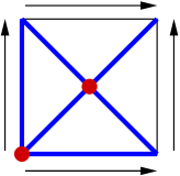
(a) The toric arrangement corresponding to the Zwart–Powell Example in $\mathbb{R}^{2}/\mathbb{Z}^{2}$

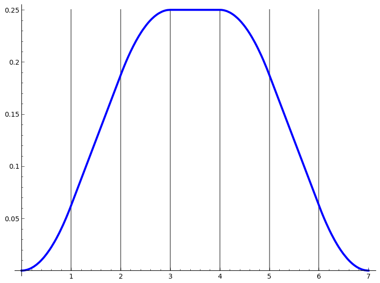
(b) The box spline defined by the list $X=(1,2,4)$

Figure 2. A toric arrangement in $\mathbb{R}^{2}/\mathbb{Z}^{2}$ and a box spline

The projections of the periodic Todd operators are:

$$\tilde{f}_{(0,0)} =1+\frac{1}{2}s_{1}+\frac{3}{2}s_{2}+\frac{3}{4}s_{1}s_{2}+s_{2}^{2}+\frac{1}{4}e_{\phi}$$

$$\tilde{f}_{(0,1)} =1+\frac{1}{2}s_{1}+\frac{1}{2}s_{2}+\frac{1}{4}s_{1}s_{2}-e_{\phi}\frac{s_{1}s_{2}}{4} \tilde{f}_{(1,1)} =1-\frac{1}{2}s_{1}+\frac{1}{2}s_{2}-\frac{1}{4}s_{1}s_{2}+e_{\phi_{1}}\frac{s_{1}s_{2}}{4}$$

$$\tilde{f}_{(0,2)} =1+\frac{1}{2}s_{1}-\frac{1}{2}s_{2}-\frac{1}{4}s_{1}s_{2}+e_{\phi_{1}}\frac{s_{1}s_{2}}{4} \tilde{f}_{(1,2)} =1-\frac{1}{2}s_{1}-\frac{1}{2}s_{2}+\frac{1}{4}s_{1}s_{2}-e_{\phi_{1}}\frac{s_{1}s_{2}}{4}$$

Example 10.2 (Zwart–Powell and the isomorphism $L:\widetilde{\mathcal{P}}(X)\to\mathbb{C}[\Lambda]/\mathop{\mathcal{J}^{\nabla}_{\mathbb{C}}\!}(X)$).

In this example we use the algorithm described in Remark 7.13 to calculate the map $L:\widetilde{\mathcal{P}}_{\mathbb{C}}(X)\to\mathbb{C}[\Lambda]/\mathop{\mathcal{J}^{\nabla}_{\mathbb{C}}\!}(X)$. Recall that $\mathbb{C}[\Lambda]\cong\mathbb{C}[a_{1}^{\pm 1},a_{2}^{\pm 1}]$ and $\operatorname{Sym}_{\mathbb{C}}(U)\cong\mathbb{C}[s_{1},\ldots,s_{d}]$.

1. The toric arrangement has two vertices: $\mathcal{V}(X)=\{(1,1),(-1,-1)\}\subseteq(\mathbb{C}^{*})^{2}$. The primary decomposition of the discrete cocircuit ideal is

   $$\mathop{\mathcal{J}^{\nabla}_{\mathbb{C}}\!}(X) =\biggl{(}(1-a_{1})(1-a_{2})(1-a_{1}a_{2}),(1-a_{1})(1-a_{2})(a_{1}-a_{2}),$$

   $$\qquad(1-a_{1})(1-a_{1}a_{2})(a_{1}-{a_{2}}),(1-a_{2})(1-a_{1}a_{2})(a_{1}-a_{2})\biggr{)}$$

   $$=\underbrace{\big{(}(a_{1}-1)^{3},(a_{1}-1)^{2}(a_{2}-1),(a_{1}-1)(a_{2}-1)^{2},(a_{2}-1)^{3}\big{)}}_{e_{\phi}=(1,1)}\cap\underbrace{\big{(}a_{1}+1,a_{2}+1\big{)}}_{e_{\phi}=(-1,-1)}.$$

2. To begin with, we consider the vertex $e_{\phi}=(-1,-1)$. We choose the representative $\theta(u_{1},u_{2})=\frac{1}{2}(u_{1}+u_{2})$. Then $\mathcal{P}_{\mathbb{C}}(X_{\phi})=\mathbb{C}\cong\operatorname{Sym}_{\mathbb{C}}(U)/\mathop{\mathcal{J}^{\partial}_{\mathbb{C}}\!}(X_{\phi})\cong\mathbb{C}[\Lambda]/\mathop{\mathcal{J}^{\nabla}_{\mathbb{C}}\!}(X)_{\phi}$. So $i_{\log}^{\theta}\circ\tau_{\theta}\circ j_{\phi}$ maps $1\in\mathcal{P}(X_{\phi})$ to $\bar{1}\in\mathbb{C}[\Lambda]/\mathop{\mathcal{J}^{\nabla}_{\mathbb{C}}\!}(X)_{\phi}$.

   Now we consider the vertex $e_{\phi}=(1,1)$. We choose the representative $\theta(u_{1},u_{2})=0$. Since $(a_{1}-1)^{3}$ and $(a_{2}-1)^{3}$ are contained in $\mathop{\mathcal{J}^{\nabla}_{\mathbb{C}}\!}(X)$, we only have to develop the logarithm up to degree $2$. Hence $i_{\log}^{\theta}(\tau_{\theta}(j_{\phi}(s_{1})))=\log(a_{1})=a_{1}-1-\frac{(a_{1}-1)^{2}}{2}=-\frac{a_{1}^{2}}{2}+2a_{1}-{\frac{3}{2}}$. Similarly, $i_{\log}^{\theta}(\tau_{\theta}(j_{\phi}(s_{2})))=-\frac{a_{2}^{2}}{2}+2a_{2}-\frac{3}{2}$. Hence, $i_{\log}^{\theta}\circ\tau_{\theta}\circ j_{\phi}$ maps $\mathcal{P}_{\mathbb{C}}(X)$ to $\mathbb{C}[\Lambda]/\mathop{\mathcal{J}^{\nabla}_{\mathbb{C}}\!}(X)_{(1,1)}$ in the following way:

   $$1 \mapsto 1 s_{1}^{2} \mapsto(a_{1}-1)^{2}$$

   $$s_{1} \mapsto-\frac{a_{1}^{2}}{2}+2a_{1}-\frac{3}{2} s_{1}s_{2} \mapsto(a_{1}-1)(a_{2}-1)$$

   $$s_{2} \mapsto-\frac{a_{2}^{2}}{2}+2a_{2}-\frac{3}{2} s_{2}^{2} \mapsto(a_{2}-1)^{2}$$

3. Now we have to find the embeddings $\kappa^{\phi}:\mathbb{C}[\Lambda]/\mathop{\mathcal{J}^{\nabla}_{\mathbb{C}}\!}(X)_{\phi}\hookrightarrow\mathbb{C}[\Lambda]/\mathop{\mathcal{J}^{\nabla}_{\mathbb{C}}\!}(X)_{\phi}$. Note that $(a_{2}^{2}-4a_{2}+7)(a_{2}+1)-(a_{2}-1)^{3}=8$. Hence $\kappa^{(1,1)}(1)=1+\frac{1}{8}(a_{2}-1)^{3}=\frac{1}{8}a_{2}^{3}-\frac{3}{8}a_{2}^{2}+\frac{3}{8}a_{2}+\frac{7}{8}$ and $\kappa^{(-1,-1)}(1)=1-\frac{1}{8}(a_{2}^{2}-4a_{2}+7)(a_{2}+1)=-\frac{1}{8}a_{2}^{3}+\frac{3}{8}a_{2}^{2}-\frac{3}{8}a_{2}+\frac{1}{8}$.

   Hence the map $L$ maps $\widetilde{\mathcal{P}}_{\mathbb{C}}(X)$ to $\mathbb{C}[\Lambda]/\mathop{\mathcal{J}^{\nabla}_{\mathbb{C}}\!}(X)$ in the following way:

   $$1 \mapsto\frac{1}{8}a_{2}^{3}-\frac{3}{8}a_{2}^{2}+\frac{3}{8}a_{2}+\frac{7}{8} s_{1}^{2} \mapsto\frac{1}{2}a_{2}^{3}+a_{1}^{2}-\frac{3}{2}a_{2}^{2}-2a_{1}+\frac{3}{2}a_{2}+\frac{1}{2}$$

   $$s_{1} \mapsto-\frac{1}{2}a_{2}^{3}-\frac{1}{2}a_{1}^{2}+\frac{3}{2}a_{2}^{2}+2a_{1}-\frac{3}{2}a_{2}-1 s_{1}s_{2} \mapsto\frac{1}{2}a_{2}^{3}+a_{1}a_{2}-\frac{3}{2}a_{2}^{2}-a_{1}+\frac{1}{2}a_{2}+\frac{1}{2}$$

   $$s_{2} \mapsto-\frac{1}{2}a_{2}^{3}+a_{2}^{2}+\frac{1}{2}a_{2}-1 s_{2}^{2} \mapsto\frac{1}{2}a_{2}^{3}-\frac{1}{2}a_{2}^{2}-\frac{1}{2}a_{2}+\frac{1}{2}$$

   $$(-1)^{u_{1}+u_{2}}s_{1}s_{2} \mapsto-\frac{1}{8}a_{2}^{3}+\frac{3}{8}a_{2}^{2}-\frac{3}{8}a_{2}+\frac{1}{8}$$

   One can easily check that the coefficients of the terms on the right-hand side always sum to $0$ except in the case of $L(1)$. This must hold because of Theorem 7.4 and the fact that ${\langle s_{1},1\rangle_{\widetilde{\mathcal{P}}}}={\langle s_{2},1\rangle_{\widetilde{\mathcal{P}}}}=\ldots=0$.

Example 10.3 (The list $X=(1,2,4)$).

Let $X=(1,2,4)$. Let $\xi_{4}$ denote the map that sends $k$ to $e^{\frac{\pi i}{2}k}$, i. e. $\xi_{4}$ is a fourth root of unity. Then $\mathcal{P}(X)=\operatorname{{{span}}}\{1,s,s^{2}\}$ and $\widetilde{\mathcal{P}}(X)=\operatorname{{{span}}}\{1,s,s^{2},\>\xi_{4}s^{2},\xi_{4}^{3}s^{2},\xi_{4}^{2}s,\xi_{4}^{2}s^{2}\}$. The elements of the internal space must satisfy $D_{s}^{2}f=0$ at the origin. Hence $\widetilde{\mathcal{P}}_{-}(X)=\{1,s,\xi_{2}s,\>(1-\xi_{4})s^{2},(\xi_{4}-\xi_{4}^{3})s^{2},(\xi_{4}^{2}-\xi_{4}^{3})s^{2}\}$.

Furthermore, $\mathcal{D}(X)=\operatorname{{{span}}}\{1,t,t^{2}\}$ and $\operatorname{DM}(X)=\operatorname{{{span}}}\{1,t,t^{2},\xi_{4},\xi_{4}^{2},\xi_{4}^{2}t,\xi_{4}^{3}\}$. The box spline is shown in Figure 2(b). Formulas for the splines and the vector partition function are:

$$B_{X}(u) =\begin{cases}\frac{1}{16}u^{2}&0\leq u\leq 1\\ \frac{1}{8}u-\frac{1}{16}&1\leq u\leq 2\\ -\frac{1}{16}u^{2}+\frac{3}{8}u-\frac{5}{16}&2\leq u\leq 3\\ \frac{1}{4}&3\leq u\leq 4\\ -\frac{1}{16}u^{2}+\frac{1}{2}u-\frac{3}{4}&4\leq u\leq 5\\ -\frac{1}{8}u+\frac{13}{16}&5\leq u\leq 6\\ \frac{1}{16}u^{2}-\frac{7}{8}u+\frac{49}{16}&6\leq u\leq 7\end{cases} \>i_{X}(u) =\begin{cases}\frac{1}{16}u^{2}+\frac{1}{2}u+1&u\equiv 0\mod 4\\ \frac{1}{16}u^{2}+\frac{3}{8}u+\frac{9}{16}&u\equiv 1\mod 4\\ \frac{1}{16}u^{2}+\frac{1}{2}u+\frac{12}{16}&u\equiv 2\mod 4\\ \frac{1}{16}u^{2}+\frac{3}{8}u+\frac{5}{16}&u\equiv 3\mod 4\\ \end{cases}$$

$$T_{X}(u) =\frac{1}{16}u^{2} \;i_{X}(u) =\frac{1}{16}u^{2}+\frac{7+\xi_{4}^{2}}{16}u+\frac{21+7\xi_{4}^{2}}{32}+\frac{1}{16}\xi_{4}(1-i)+\frac{1}{16}\xi_{4}^{3}(1+i)$$

The projection of $\operatorname{{T}\widetilde{{od}}{d}}(X,0)$ is

$$\tilde{p}_{0} =1+\frac{7}{2}s+\frac{21}{4}s^{2}+\xi_{4}(\frac{1}{2}-\frac{1}{2}i)s^{2}+\xi_{4}^{3}(\frac{1}{2}+\frac{1}{2}i)s^{2}+\xi_{4}^{2}(\frac{1}{2}s+\frac{7}{4}s^{2}).$$

$$\operatorname{{T}\widetilde{{od}}{d}^{box}}(X) =1+\frac{7}{2}s+\frac{21}{4}s^{2}+\xi_{4}(\frac{1}{2}-\frac{1}{2}i)s^{2}\frac{(1+i\tau_{1})(1+\tau_{2})}{(1-\tau_{1})(1-\tau_{2})}$$

$$\qquad+\xi_{4}^{3}(\frac{1}{2}+\frac{1}{2}i)s^{2}\frac{(1-i\tau_{1})(1+\tau_{2})}{(1-\tau_{1})(1-\tau_{2})}+\xi_{2}(\frac{1}{2}s+\frac{7}{4}s^{2})\frac{(1+\tau_{1})}{(1-\tau_{1})}$$

is the operator defined in Remark 5.11.

The arithmetic Tutte polynomial is ${\mathfrak{M}}_{X}(\alpha,\beta)=(\alpha-1)+7+4(\beta-1)+(\beta-1)^{2}=\alpha+\beta^{2}+2\beta+3$. Hence $q^{2}{\mathfrak{M}}_{X}(0,q^{-1})=1+2q+3q^{2}=\operatorname{{{Hilb}}}(\widetilde{\mathcal{P}}_{-}(X),q)$ and $q^{2}{\mathfrak{M}}_{X}(1,q^{-1})=1+2q+4q^{2}=\operatorname{{{Hilb}}}(\widetilde{\mathcal{P}}(X),q)$.

Example 10.4 (The list $X=(1,2,4)$ and the isomorphism $L$).

The primary decomposition of the discrete cocircuit ideal is

$$\mathop{\mathcal{J}^{\nabla}_{\mathbb{C}}\!}(X) =\operatorname{{{ideal}}}\{(1-a)(1-a^{2})(1-a^{4})\}$$ (76)

$$=\operatorname{{{ideal}}}\{(a-1)^{3}\}\cap\operatorname{{{ideal}}}\{(a+1)^{2}\}\cap\operatorname{{{ideal}}}\{a-i\}\cap\operatorname{{{ideal}}}\{a+i\}.$$ (77)

The toric arrangement has four vertices: $\mathcal{V}(X)=\{1,i,-1,-i\}\subseteq\mathbb{C}^{*}$. They can be represented by $\theta=0,\frac{1}{4},\frac{1}{2},\frac{3}{4}$. One obtains that $i_{\log}^{0}(\tau_{0}(j_{1}(s)))=-\frac{a^{2}}{2}+2a-\frac{3}{2}$, $i_{\log}^{0}(\tau_{0}(j_{1}(s^{2})))=a^{2}-2a+1$, and $i_{\log}^{\frac{1}{2}}(\tau_{\frac{1}{2}}(j_{-1}(s)))=-a-1$. For $\theta\in\{\frac{1}{4},\frac{3}{4}\}$, the spaces are trivial and $i_{\log}^{\theta}\circ\tau_{\theta}\circ j_{\phi}$ just maps $1$ to $\bar{1}$.

Now if we lift these elements we obtain that the map $L$ maps $\widetilde{\mathcal{P}}_{\mathbb{C}}(X)$ to $\mathbb{C}[\Lambda]/\mathop{\mathcal{J}^{\nabla}_{\mathbb{C}}\!}(X)$ in the following way:

$$1 \mapsto\frac{9}{32}a^{6}-\frac{1}{4}a^{5}-\frac{13}{32}a^{4}+\frac{1}{4}a^{3}-\frac{1}{32}a^{2}+\frac{1}{2}a+\frac{21}{32}$$

$$s \mapsto-\frac{5}{16}a^{6}+\frac{1}{8}a^{5}+\frac{7}{16}a^{4}+\frac{5}{16}a^{2}-\frac{1}{8}a-\frac{7}{16}$$

$$s^{2} \mapsto\frac{1}{8}a^{6}-\frac{1}{8}a^{4}-\frac{1}{8}a^{2}+\frac{1}{8}$$

$$\xi_{4}^{2}s \mapsto-\frac{5}{32}a^{6}+\frac{1}{4}a^{5}+\frac{1}{32}a^{4}-\frac{1}{4}a^{3}+\frac{13}{32}a^{2}-\frac{1}{2}a+\frac{7}{32}$$

$$\xi_{4}^{2}s^{2} \mapsto\frac{1}{16}a^{6}-\frac{1}{8}a^{5}+\frac{1}{16}a^{4}-\frac{1}{16}a^{2}+\frac{1}{8}a-\frac{1}{16}$$

$$\xi_{4}s^{2} \mapsto\left(\frac{1}{16}i-\frac{1}{16}\right)a^{6}-\frac{1}{8}ia^{5}+\left(-\frac{1}{16}i+\frac{3}{16}\right)a^{4}+\frac{1}{4}ia^{3}+\left(-\frac{1}{16}i-\frac{3}{16}\right)a^{2}-\frac{1}{8}ia+\frac{1}{16}i+\frac{1}{16}$$

$$\xi_{4}^{3}s^{2} \mapsto\left(-\frac{1}{16}i-\frac{1}{16}\right)a^{6}+\frac{1}{8}ia^{5}+\left(\frac{1}{16}i+\frac{3}{16}\right)a^{4}-\frac{1}{4}ia^{3}+\left(\frac{1}{16}i-\frac{3}{16}\right)a^{2}+\frac{1}{8}ia-\frac{1}{16}i+\frac{1}{16}$$

10.2. Examples involving torsion and deletion-contraction

Figure 3. A toric arrangement in $T(\mathbb{Z}\oplus\mathbb{Z}/3\mathbb{Z})\cong S^{1}\times\mathbb{Z}/3\mathbb{Z}$.

Example 10.5 (A toric arrangement on a disconnected torus).

$$\text{Let }X=\begin{pmatrix}4&2&1&0\\ \bar{0}&\bar{1}&\bar{2}&\bar{1}\end{pmatrix}=(x_{1},x_{2},x_{3},x_{4})\subseteq\mathbb{Z}\oplus\mathbb{Z}/3\mathbb{Z}.$$ (78)

Note that $T(\mathbb{Z}\oplus\mathbb{Z}/3\mathbb{Z})\cong S^{1}\times\{g_{3}^{0},g_{3}^{1},g_{3}^{2}\}$, where $(\alpha,g_{3}^{k})$ maps $(a,\bar{b})$ to $\alpha^{a}\cdot e^{2\pi i\frac{k}{3}}$ for $\alpha\in S^{1}\subseteq\mathbb{C}$, $k\in\{0,1,2\}$, $a\in\mathbb{Z}$ and $\bar{b}\in\mathbb{Z}/3\mathbb{Z}$.

The corresponding toric arrangement is shown in Figure 3. $x_{1}$ defines the twelve (small) cyan vertices. $x_{2}$ defines the six (medium sized) blue vertices and $x_{3}$ defines the three (large) green vertices. Note that $\operatorname{rk}(x_{4})=0$, hence $x_{4}$ does not define a vertex but a one-dimensional hypersurface, the leftmost (red) copy of the $S^{1}$.

Example 10.6.

Let $X=\begin{pmatrix}2&4&0&-1\\ 0&1&2&1\end{pmatrix}$. Note that $\left|\mathcal{V}(X)\right|=14$ (see Figure 4) and $\dim\widetilde{\mathcal{P}}(X)=23$. Some of the differential equations that have to be satisfied by the elements of $\widetilde{\mathcal{P}}_{-}(X)$ are $D_{s_{1}}^{2}p(0,\cdot)=D_{s_{2}}^{2}p(0,\cdot)=D_{s_{1}}D_{s_{2}}p(0,\cdot)=D_{s_{2}}^{2}p((1,0),\cdot)=D_{s_{1}}^{2}p((0,1),\cdot)=0$. We leave it to the reader to calculate $\widetilde{\mathcal{P}}(X)$ and $\widetilde{\mathcal{P}}_{-}(X)$.

Let $x=(2,0)$ be the first column. Then $X/x=((\bar{0},1),(\bar{0},2),(\bar{1},1))\subseteq\mathbb{Z}/2\mathbb{Z}\oplus\mathbb{Z}$ and $\mathcal{V}(X/x)=\{1,(-1)^{b},(-1)^{\bar{a}},(-1)^{\bar{a}+b}\}$. The differential equations for the internal space are $D_{s_{2}}^{2}p((\bar{0},0),\cdot)=D_{s_{2}}^{2}p((\bar{1},0),\cdot)=0$. Hence

$$\widetilde{\mathcal{P}}(X/x) =\{1,\,s_{2},\,s_{2}^{2},(-1)^{b}s_{2},\,(-1)^{b}s_{2}^{2},\,(-1)^{\bar{a}}s_{2}^{2},\,(-1)^{\bar{a}+b}s_{2},\,(-1)^{\bar{a}+b}s_{2}^{2}\}\text{ and}$$

$$\widetilde{\mathcal{P}}_{-}(X/x) =\{1,\,s_{2},\,(-1)^{b}s_{2},\,(-1)^{\bar{a}+b}s_{2},\,s_{2}^{2}-(-1)^{b}s_{2}^{2},\,(-1)^{\bar{a}}s_{2}^{2}-(-1)^{\bar{a}+b}s_{2}^{2}\}.$$

In general, it is non-trivial to find preimages of elements of $\widetilde{\mathcal{P}}_{-}(X/x)$ in $\widetilde{\mathcal{P}}_{-}(X)$. For example, can you find an element of $\pi_{x}^{-1}(s_{2}^{2}+(-1)^{\bar{a}}2s_{2}^{2}-(-1)^{b}s_{2}^{2}-(-1)^{\bar{a}+b}2s_{2}^{2})$? This may help you to do so:

$$\tilde{f}_{(0,1)} =\frac{9}{4}s_{1}^{2}+\frac{9}{4}s_{1}s_{2}+\frac{1}{4}s_{2}^{2}+\frac{5}{2}s_{1}+s_{2}+1+(-1)^{a}(-\frac{5}{4}s_{1}^{2}+\frac{3}{4}s_{1}s_{2}+\frac{1}{2}s_{2}^{2}-\frac{1}{2}s_{1}+\frac{1}{2}s_{2})$$

$$\quad-(-1)^{b}(-s_{1}^{2}+\frac{3}{4}s_{1}s_{2}+\frac{1}{4}s_{2}^{2})-(-1)^{a+b}(5s_{1}^{2}+\frac{13}{4}s_{1}s_{2}+\frac{1}{2}s_{2}^{2}+2s_{1}+\frac{1}{2}s_{2})+\ldots$$

$$\pi_{x}(\tilde{f}_{(0,1)}) =\frac{1}{4}s_{2}^{2}+s_{2}+1+(-1)^{\bar{a}}(\frac{1}{2}s_{2}^{2}+\frac{1}{2}s_{2})-(-1)^{b}\frac{1}{4}s_{2}^{2}-(-1)^{\bar{a}+b}(\frac{1}{2}s_{2}^{2}+\frac{1}{2}s_{2})$$ (79)

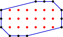
Figure 4. On the left: the toric arrangement in Example 10.6 drawn in $\mathbb{R}^{2}/\mathbb{Z}^{2}$. The three vertices that are circled have a non-trivial $\mathcal{P}$-space attached to it. In the middle: the projection to $T(\mathbb{Z}\oplus\mathbb{Z}/2\mathbb{Z})$. On the right: the zonotope.

Appendix A Commands for sage and Singular

In this appendix we explain how Examples 10.2 and 10.4 can be calculated using computer algebra programs. We use the algorithm described in Remark 7.13. Most of the calculations can be done in Sage [44] which uses Singular [27] for some of the calculations.

Here is the code for the Zwart-Powell element (Example 10.2):

sage: K.<j> = QQ[I]
sage: R.<a,b> = K[]   # the polynomial ring in two variables over the field Q[i]
sage: J = ideal((1-a)*(1-b)*(1-a*b), (1-a)*(1-b)*(a-b), (1-a)*(a-b)*(1-a*b),
(1-b)*(a-b)*(1-a*b)) # the discrete cocircuit ideal
sage: J.variety() # the points defined by the ideal
[{a: -1, b: -1}, {a: 1, b: 1}]
sage: [J1,J2] = J.primary_decomposition() # the primary decomposition
sage: J1
Ideal (b^3 - 3*b^2 + 3*b - 1, a*b^2 - 2*a*b - b^2 + a + 2*b - 1,
a^2*b - a^2 - 2*a*b + 2*a + b - 1, a^3 - 3*a^2 + 3*a - 1) of Multivariate Polynomial Ring
in a, b over Number Field in I with defining polynomial x^2 + 1
sage: J2
Ideal (b + 1, a + 1) of Multivariate Polynomial Ring
in a, b over Number Field in I with defining polynomial x^2 + 1
sage: f1 = (a-1) - (a-1)**2/2  # the image of s1 under tau and the logarithmic isomorphism
sage: f2 = (b-1) - (b-1)**2/2  # the image of s2 under tau and the logarithmic isomorphism
sage: J1.reduce(f1*f1) # f1*f1 reduced modulo the ideal J1
a^2 - 2*a + 1
sage: J1.reduce(f1*f2)
a*b - a - b + 1
sage: J1.reduce(f2*f2)
b^2 - 2*b + 1
sage: g1 = 1+1/8*(a-1)**3 # the lifting of 1 in C[a,b]/J1 to C[a,b]/J
sage: J.reduce(g1)
1/8*b^3 - 3/8*b^2 + 3/8*b + 7/8
sage: J.reduce(g1*f1)
-1/2*b^3 - 1/2*a^2 + 3/2*b^2 + 2*a - 3/2*b - 1
sage: J.reduce(g1*f2)
-1/2*b^3 + b^2 + 1/2*b - 1
sage: J.reduce(g1*f1**2)
1/2*b^3 + a^2 - 3/2*b^2 - 2*a + 3/2*b + 1/2
sage: J.reduce(g1*f1*f2)
1/2*b^3 + a*b - 3/2*b^2 - a + 1/2*b + 1/2
sage: J.reduce(g1*f2**2)
1/2*b^3 - 1/2*b^2 - 1/2*b + 1/2

The equation $(a_{2}^{2}-4a_{2}+7)(a_{2}+1)-(a_{2}-1)^{3}=8$ can be found using the liftstd function of Singular [27]:

> ring r = 0,(a,b),dp;
> ideal J1 = (1-a)**3, (1-a)**2*(1-b), (1-a)*(1-b)**2, (1-b)**3;
> ideal J2 = a + 1, b + 1;
> matrix T;
> def sm = liftstd(J1 + J2, T);
> sm;
sm[1]=8
> T;
T[1,1]=0
T[2,1]=0
T[3,1]=0
T[4,1]=1
T[5,1]=0
T[6,1]=b2-4b+7
> matrix(J1+J2)
_[1,1]=-a3+3a2-3a+1
_[1,2]=-a2b+a2+2ab-2a-b+1
_[1,3]=-ab2+2ab+b2-a-2b+1
_[1,4]=-b3+3b2-3b+1
_[1,5]=a+1
_[1,6]=b+1
> matrix(J1+J2)*T; // This gives us the equation above
_[1,1]=8

Here is the code for the list $X=(1,2,4)$ (Example 10.4):

sage: K.<j> = QQ[I]
sage: R = sage.rings.polynomial.multi_polynomial_libsingular.
MPolynomialRing_libsingular(K, 1, (’a’,), TermOrder(’degrevlex’,1))
# we have to tell sage that we want to use Singular
# otherwise, primary decomposition is not available for polynomial rings in one variable
sage: R.inject_variables()
Defining a
sage: R
Multivariate Polynomial Ring in a over Number Field in I with defining polynomial x^2 + 1
sage: J= ideal( (1-a)*(1-a**2)*(1-a**4)) # the discrete cocircuit ideal
sage:  J.primary_decomposition()
[Ideal (a^3 - 3*a^2 + 3*a - 1) of Multivariate Polynomial Ring
 in a, b over Number Field in I with defining polynomial x^2 + 1,
 Ideal (a^2 + 2*a + 1) of Multivariate Polynomial Ring
 in a, b over Number Field in I with defining polynomial x^2 + 1,
 Ideal (a + (I)) of Multivariate Polynomial Ring
 in a, b over Number Field in I with defining polynomial x^2 + 1,
 Ideal (a + (-I)) of Multivariate Polynomial Ring
 in a, b over Number Field in I with defining polynomial x^2 + 1]
sage: R.<a> = K[] # change the implementation of the ring, otherwise CRT_list does not work
sage: J  = ideal( (1-a)*(1-a**2)*(1-a**4)) # the discrete cocircuit ideal
sage: J1 = ideal( (a-1)**3 )  # the ideal corresponding to the vertex 1
sage: J2 = ideal( (a+1)**2 ) # the ideal corresponding to the vertex -1
sage: g1 = CRT_list( [ 1, 0, 0, 0], [ (a-1)**3, (a+1)**2, (a+j), (a-j) ] )
sage: g2 = CRT_list( [ 0, 1, 0, 0], [ (a-1)**3, (a+1)**2, (a+j), (a-j) ] )
sage: g3 = CRT_list( [ 0, 0, 1, 0], [ (a-1)**3, (a+1)**2, (a+j), (a-j) ] )
sage: g4 = CRT_list( [ 0, 0, 0, 1], [ (a-1)**3, (a+1)**2, (a+j), (a-j) ] )
sage: [g1,g2,g3,g4]
[9/32*a^6 - 1/4*a^5 - 13/32*a^4 + 1/4*a^3 - 1/32*a^2 + 1/2*a + 21/32,
 -5/32*a^6 + 1/4*a^5 + 1/32*a^4 - 1/4*a^3 + 13/32*a^2 - 1/2*a + 7/32,
 (-1/16*I - 1/16)*a^6 + 1/8*I*a^5 + (1/16*I + 3/16)*a^4
 - 1/4*I*a^3 + (1/16*I - 3/16)*a^2 + 1/8*I*a - 1/16*I + 1/16,
 (1/16*I - 1/16)*a^6 - 1/8*I*a^5 + (-1/16*I + 3/16)*a^4
 + 1/4*I*a^3 + (-1/16*I - 3/16)*a^2 - 1/8*I*a + 1/16*I + 1/16]
sage: f1 = -a**2/2 + 2*a - 3/2 # the image of s under the iota map for vertex 1
sage: f2 = -a -1
sage: f1**2
1/4*a^4 - 2*a^3 + 11/2*a^2 - 6*a + 9/4
sage: J1.reduce(f1**2)
a^2 - 2*a + 1
sage: J1.reduce(f1**3)
0
sage: J2.reduce(f2**2)
0
sage: [g1, J.reduce( g1 * f1), J.reduce( g1 * f1**2) ]    # generators corresponding
# to the space at vertex 1
[9/32*a^6 - 1/4*a^5 - 13/32*a^4 + 1/4*a^3 - 1/32*a^2 + 1/2*a + 21/32,
 -5/16*a^6 + 1/8*a^5 + 7/16*a^4 + 5/16*a^2 - 1/8*a - 7/16,
 1/8*a^6 - 1/8*a^4 - 1/8*a^2 + 1/8]
sage: [g2, J.reduce(g2 * f2)] # generators corresponding to the space at vertex -1
[-5/32*a^6 + 1/4*a^5 + 1/32*a^4 - 1/4*a^3 + 13/32*a^2 - 1/2*a + 7/32,
 1/16*a^6 - 1/8*a^5 + 1/16*a^4 - 1/16*a^2 + 1/8*a - 1/16]
sage: J.reduce(g2**2)
-5/32*a^6 + 1/4*a^5 + 1/32*a^4 - 1/4*a^3 + 13/32*a^2 - 1/2*a + 7/32
# note that this is equal to g2
sage: g3 # generator corresponding to the space at vertex -i
(-1/16*I - 1/16)*a^6 + 1/8*I*a^5 + (1/16*I + 3/16)*a^4 - 1/4*I*a^3
+ (1/16*I - 3/16)*a^2 + 1/8*I*a - 1/16*I + 1/16
sage: g4 # generator corresponding to the space at vertex i
(1/16*I - 1/16)*a^6 - 1/8*I*a^5 + (-1/16*I + 3/16)*a^4 + 1/4*I*a^3
 + (-1/16*I - 3/16)*a^2 - 1/8*I*a + 1/16*I + 1/16
sage: J.reduce(f2*g2)
1/16*a^6 - 1/8*a^5 + 1/16*a^4 - 1/16*a^2 + 1/8*a - 1/16
sage: 1/16*6 + 1/8*5 + 1/16*4 - 1/16*2 - 1/8
1
# < L( e_{-1} s s), e_{-1} t>_\nabla = s(D) t = 1
sage: [g1.substitute({a:1}), (J.reduce(g1*f1)).substitute({a:1}),
 (J.reduce(g1*f1**2)).substitute({a:1}), g2.substitute({a:1}),
 (J.reduce(g2*f2**2)).substitute({a:1}), g3.substitute({a:1}), g4.substitute({a:1})]
[1, 0, 0, 0, 0, 0, 0]
 # another check: < L( p ), 1 >_\nabla = 1 iff p = 1

References

- [1] A. A. Akopyan and A. A. Saakyan, A system of differential equations that is related to the polynomial class of translates of a box spline, Mat. Zametki 44 (1988), no. 6, 705–724, 861.
- [2] Federico Ardila and Alexander Postnikov, Combinatorics and geometry of power ideals, Trans. Amer. Math. Soc. 362 (2010), no. 8, 4357–4384.
- [3] by same author, Two counterexamples for power ideals of hyperplane arrangements, 2012, arXiv:1211.1368, to appear in Trans. Amer. Math. Soc. as a correction to [2].
- [4] Matthias Beck and Sinai Robins, Computing the continuous discretely. integer-point enumeration in polyhedra., Undergraduate Texts in Mathematics, Springer, New York, 2007.
- [5] Asher Ben-Artzi and Amos Ron, Translates of exponential box splines and their related spaces, Trans. Amer. Math. Soc. 309 (1988), no. 2, 683–710.
- [6] Andrew Berget, Products of linear forms and Tutte polynomials, European J. Combin. 31 (2010), no. 7, 1924–1935.
- [7] Arzu Boysal and Michèle Vergne, Paradan’s wall crossing formula for partition functions and Khovanski-Pukhlikov differential operator, Ann. Inst. Fourier (Grenoble) 59 (2009), no. 5, 1715–1752.
- [8] Petter Brändén and Luca Moci, The multivariate arithmetic Tutte polynomial, Trans. Amer. Math. Soc. 366 (2014), no. 10, 5523–5540.
- [9] Michel Brion and Michèle Vergne, Residue formulae, vector partition functions and lattice points in rational polytopes, J. Amer. Math. Soc. 10 (1997), no. 4, 797–833.
- [10] by same author, Arrangement of hyperplanes. I. Rational functions and Jeffrey-Kirwan residue, Ann. Sci. École Norm. Sup. (4) 32 (1999), no. 5, 715–741.
- [11] Francesco Cavazzani and Luca Moci, Geometric realizations and duality for Dahmen-Micchelli modules and De Concini-Procesi-Vergne modules, 2012, arXiv:1303.0902.
- [12] David A. Cox, John Little, and Donal O’Shea, Using algebraic geometry, second ed., Graduate Texts in Mathematics, vol. 185, Springer, New York, 2005.
- [13] David A. Cox, John B. Little, and Henry K. Schenck, Toric varieties, Graduate Studies in Mathematics, vol. 124, American Mathematical Society, Providence, RI, 2011.
- [14] Michele D’Adderio and Luca Moci, Ehrhart polynomial and arithmetic Tutte polynomial, European J. Combin. 33 (2012), no. 7, 1479 – 1483.
- [15] Michele D’Adderio and Luca Moci, Arithmetic matroids, the Tutte polynomial and toric arrangements, Adv. Math. 232 (2013), no. 1, 335–367.
- [16] Wolfgang Dahmen and Charles A. Micchelli, On the local linear independence of translates of a box spline, Studia Math. 82 (1985), no. 3, 243–263.
- [17] by same author, On the solution of certain systems of partial difference equations and linear dependence of translates of box splines, Trans. Amer. Math. Soc. 292 (1985), no. 1, 305–320.
- [18] Carl de Boor, Nira Dyn, and Amos Ron, On two polynomial spaces associated with a box spline, Pacific J. Math. 147 (1991), no. 2, 249–267.
- [19] Carl de Boor and Klaus Höllig, -splines from parallelepipeds, J. Analyse Math. 42 (1982/83), 99–115.
- [20] Carl de Boor, Klaus Höllig, and Sherman D. Riemenschneider, Box splines, Applied Mathematical Sciences, vol. 98, Springer-Verlag, New York, 1993.
- [21] Corrado De Concini and Claudio Procesi, Topics in hyperplane arrangements, polytopes and box-splines, Universitext, Springer, New York, 2011.
- [22] Corrado De Concini, Claudio Procesi, and Michèle Vergne, Vector partition functions and index of transversally elliptic operators, Transform. Groups 15 (2010), no. 4, 775–811.
- [23] by same author, Infinitesimal index: cohomology computations, Transformation Groups 16 (2011), no. 3, 717–735 (English).
- [24] by same author, Box splines and the equivariant index theorem, J. Inst. Math. Jussieu 12 (2013), 503–544.
- [25] by same author, The infinitesimal index, J. Inst. Math. Jussieu 12 (2013), no. 2, 297–334.
- [26] Jesús A. De Loera, The many aspects of counting lattice points in polytopes, Math. Semesterber. 52 (2005), no. 2, 175–195.
- [27] Wolfram Decker, Gert-Martin Greuel, Gerhard Pfister, and Hans Schönemann, Singular 3-1-6 — A computer algebra system for polynomial computations, http://www.singular.uni-kl.de, 2012.
- [28] Nira Dyn and Amos Ron, Local approximation by certain spaces of exponential polynomials, approximation order of exponential box splines, and related interpolation problems, Trans. Amer. Math. Soc. 319 (1990), no. 1, 381–403.
- [29] David Eisenbud, Commutative algebra with a view toward algebraic geometry, Graduate Texts in Mathematics, vol. 150, Springer-Verlag, New York, 1995.
- [30] Friedrich Hirzebruch, Neue topologische Methoden in der algebraischen Geometrie, Ergebnisse der Mathematik und ihrer Grenzgebiete (N.F.), Heft 9, Springer-Verlag, Berlin, 1956.
- [31] Olga Holtz and Amos Ron, Zonotopal algebra, Adv. Math. 227 (2011), no. 2, 847–894.
- [32] Olga Holtz, Amos Ron, and Zhiqiang Xu, Hierarchical zonotopal spaces, Trans. Amer. Math. Soc. 364 (2012), no. 2, 745–766.
- [33] Rong-Qing Jia, Subspaces invariant under translations and dual bases for box splines., Chin. Ann. Math., Ser. A 11 (1990), no. 6, 733–743 (Chinese).
- [34] Askold Khovanskiĭ and Aleksandr Pukhlikov, The Riemann-Roch theorem for integrals and sums of quasipolynomials on virtual polytopes, Algebra i Analiz 4 (1992), no. 4, 188–216.
- [35] Serge Lang, Algebra, third ed., Graduate Texts in Mathematics, vol. 211, Springer-Verlag, New York, 2002.
- [36] Matthias Lenz, Hierarchical zonotopal power ideals, European J. Combin. 33 (2012), no. 6, 1120–1141.
- [37] by same author, Splines, lattice points, and (arithmetic) matroids, Proceedings of 26th International Conference on Formal Power Series and Algebraic Combinatorics (FPSAC 2014), DMTCS Proceedings, Assoc. Discrete Math. Theor. Comput. Sci., Nancy, France, 2014, pp. 49–60.
- [38] by same author, Interpolation, box splines, and lattice points in zonotopes, International Mathematics Research Notices (first published online July 10, 2013), 16 pages.
- [39] by same author, Lattice points in polytopes, box splines, and Todd operators, International Mathematics Research Notices (first published online June 12, 2014), 22 pages.
- [40] Luca Moci, A Tutte polynomial for toric arrangements, Trans. Amer. Math. Soc. 364 (2012), no. 2, 1067–1088.
- [41] Peter Orlik and Hiroaki Terao, Commutative algebras for arrangements, Nagoya Math. J. 134 (1994), 65–73.
- [42] James G. Oxley, Matroid theory, Oxford Science Publications, The Clarendon Press Oxford University Press, New York, 1992.
- [43] Richard P. Stanley, An introduction to hyperplane arrangements, Geometric combinatorics, IAS/Park City Math. Ser., vol. 13, Amer. Math. Soc., Providence, RI, 2007, pp. 389–496.
- [44] W. A. Stein et al., Sage Mathematics Software (Version 6.2), The Sage Development Team, 2014, http://www.sagemath.org.
- [45] András Szenes and Michèle Vergne, Residue formulae for vector partitions and Euler-MacLaurin sums, Adv. in Appl. Math. 30 (2003), no. 1-2, 295–342, Formal power series and algebraic combinatorics (Scottsdale, AZ, 2001).
- [46] Michèle Vergne, Residue formulae for Verlinde sums, and for number of integral points in convex rational polytopes, European women in mathematics (Malta, 2001), World Sci. Publ., River Edge, NJ, 2003, pp. 225–285.
- [47] Ren-Hong Wang, Multivariate spline and algebraic geometry, J. Comput. Appl. Math. 121 (2000), no. 1-2, 153–163, Numerical analysis in the 20th century, Vol. I, Approximation theory.