Construction of Tight Frames on Graphs and Application to Denoising

Abstract

Given a neighborhood graph representation of a finite set of points $x_{i}\in\mathbb{R}^{d},i=1,\ldots,n,$ we construct a frame (redundant dictionary) for the space of real-valued functions defined on the graph. This frame is adapted to the underlying geometrical structure of the $x_{i}$, has finitely many elements, and these elements are localized in frequency as well as in space. This construction follows the ideas of Hammond11 , with the key point that we construct a tight (or Parseval) frame. This means we have a very simple, explicit reconstruction formula for every function $f$ defined on the graph from the coefficients given by its scalar product with the frame elements. We use this representation in the setting of denoising where we are given noisy observations of a function $f$ defined on the graph. By applying a thresholding method to the coefficients in the reconstruction formula, we define an estimate of $f$ whose risk satisfies a tight oracle inequality.

1 Introduction

1.1 Motivation

When dealing with high-dimensional data, a general principle is that the curse of dimensionality can be efficiently fought if one assumes the data points to lie on a structure of smaller intrinsic dimensionality, typically a manifold. Some well-known methods to discover such a lower dimensional structure include Isomap isomap00 , LLE lle00 and Laplacian Eigenmaps lap_eig03 .

In this work, our main interest is not in visualizing or representing by an explicit mapping the underlying structure of the observed data points; rather, we want to represent or estimate efficiently a real-valued function on these points. More specifically, we focus on the following denoising problem: assuming we observe a noisy version of the function $f$, $y_{i}=f(x_{i})+\varepsilon_{i}$ at points $(x_{1},\ldots,x_{n})$, we would like to recover the values of $f$ at these points. An important step for solving this problem is to find a dictionary of functions to represent the signal $f$, which is adapted to the structure of the data. Ideally, we would like this dictionary to exhibit the features of a wavelet basis. In traditional signal processing on a flat space, with data points on a regular grid, orthogonal wavelet bases offer a very powerful tool to sparsely represent signals with inhomogeneous regularity (such as a signal that is very smooth everywhere except at a few singular points where it is discontinuous). Such bases are in particular well suited to the denoising task. Can this be generalized to irregularly scattered data on a manifold?

We present such a method to construct a so-called Parseval frame of functions exhibiting wavelet-like properties while adapting to the intrinsic geometry of the data. Furthermore, we use this dictionary for the denoising task using a simple coefficient thresholding method.

This work is organized as follows. In the coming section, we discuss the relationship to previous work on which the present paper is built, as well as pointing out our new contributions. In Section 2, we recall important notions of frame theory as well as of neighborhood graphs needed for our construction. The construction of the frame and its properties is presented in Section 3. In Section 4, we develop a coefficient thresholding strategy for the denoising problem. In Section 5, we present numerical results and method comparison on testbed data.

1.2 Relation to previous work

Regression methods that adapt to an underlying lower dimension of the data have been considered by BiLi ; KpoDas ; Kpo using local polynomial estimates, random projection trees, and nearest-neighbors, respectively. However, these methods are not constructed to adapt to an inhomogeneous regularity of the target function: in these three cases, the smoothing scale (determined by the smoothing kernel bandwidth, the tree partition’s average data diameter, or the number of neighbors, respectively) is fixed globally. In the experimental section 4, for data lying on a smooth manifold but a target function exhibiting a sharp discontinuity, we demonstrate the advantage of our method over kernel smoothing.

Based on motivations similar to ours, a method for constructing a wavelet-like basis on scattered data was proposed by Gavish10 . It is based on a hierarchical tree partition of the data, on which a Haar-like basis of 0-1 functions is constructed. However, the performance of that method is then adapted to the geometry of the tree, in the sense that the distance of two points is measured through tree path distance. This can strongly distort the original distance: two close points in original distance can find themselves in very separated subtrees.

The construction proposed here, based on a transform of the spectral decomposition of the graph Laplacian, follows closely the ideas of Hammond11 . Two important contributions brought forth in the present work are that we construct a Parseval (or tight) frame, rather than a general frame; and we consider an explicit thresholding method for the denoising problem. The former point is crucial to obtain sharp bounds for the thresholding method, and also eliminates the computational problem of signal reconstruction from the frame coefficients, since Parseval frames enjoy a reconstruction formula similar to that of an orthonormal basis. The choice of multiscale bandpass filter functions leading to the tight frame is inspired by the recent work of gerard , where the spectral decomposition principle is also studied, albeit in the setting of a quite general metric space.

2 Notations - Basics

2.1 Setting

We consider a sample of $n$ points $x_{i}\in\mathbb{R}^{d}$. These points are assumed to belong to an unknown low-dimensional submanifold $\mathcal{M}\subset\mathbb{R}^{d}$. We denote the design by $\mathfrak{D}=\{x_{1},\ldots,x_{n}\}\subset\mathcal{M}$. Furthermore, we observe on these points the (noisy) value of a function $f:\mathfrak{D}\rightarrow\mathbb{R}$. Since $\mathfrak{D}$ is finite, we can represent the function $f$ as vector $f=(f(x_{1}),\ldots,f(x_{n}))^{t}\in\mathbb{R}^{n}$. The space of all (square-integrable) functions $f$ defined on $\mathfrak{D}$ is denoted $L^{2}(\mathfrak{D})$ and endowed with the usual Euclidean inner product.

We denote by $y_{i}=f(x_{i})+\epsilon_{i}$ the noisy observation of $f$ at $x_{i}$, where $\epsilon_{i}$ are independent identically distributed centered random variables. The problem we consider in this work is that of denoising, that is, try to recover the underlying value of the function $f$ at the points $x_{i}$.

While the existence of a low-dimensional supporting manifold $\mathcal{M}$ for the design points motivates the construction of the proposed method, we underline (again) that $\mathcal{M}$ is not known to the user and the method only uses the knowledge of the design points. In such a setting, a key idea to recover implicitely some information on the geometry of $\mathcal{M}$ is to construct a neighborhood graph based on the design points (see Section 2.3 for details).

2.2 Frames

For the construction in Section 3, we rely on the notion of a vector frame, for which we recall here some important properties (see e.g. FF2012 , Han07 and Christensen08 ). A frame is an overcomplete dictionary with particular properties allowing it to act almost as basis.

Definition 1

Let $\mathcal{H}$ be a Hilbert space. Then a countable set $\{z_{i}\}_{i\in I}\subset\mathcal{H}$ is a frame with frame bounds $A$ and $B$ for $\mathcal{H}$ if there exists constants $0<A\leq B<\infty$ such that

$$\forall z\in\mathcal{H}:~{}\;A\left\lVert z\right\rVert^{2}\leq\sum_{i\in I}\left\lvert\left\langle z,z_{i}\right\rangle\right\rvert^{2}\leq B\left\lVert z\right\rVert^{2}.$$ (1)

A frame is called tight if $A=B$, in particular the frame is called Parseval if $A=B=1$.

In the remainder of this work we consider the case of a Euclidean space $\mathcal{H}=\mathbb{R}^{n}$, and assume that $\{z_{i}\}_{i\in I}$ is a frame with a finite number of elements. Two important operators associated to the frame are the analysis operator

$$T:\mathbb{R}^{n}\rightarrow\mathbb{R}^{I},~{}Tz:=(\left\langle z,z_{i}\right\rangle)_{i\in I}$$ (2)

(sequence of frame coefficients), and its adjoint the synthesis operator:

$$T^{*}:\mathbb{R}^{I}\rightarrow\mathbb{R}^{n},~{}T^{*}a=T^{*}(a_{i})_{i\in I}^{t}=\sum_{i\in I}a_{i}z_{i}.$$ (3)

Further, the frame operator is defined as $S=T^{*}T$:

$$S:\mathbb{R}^{n}\rightarrow\mathcal{\mathbb{R}}^{n},~{}Sz=T^{*}Tz=\sum_{i\in I}\left\langle z,z_{i}\right\rangle z_{i},$$ (4)

and finally the Gramian operator as $U=TT^{*}$,

$$U:\mathbb{R}^{I}\rightarrow\mathbb{R}^{I},~{}Ua=TT^{*}a=\left\{\left\langle\sum_{i\in I}a_{i}z_{i},z_{k}\right\rangle\right\}_{k\in I}.$$ (5)

In matrix form, the columns of $T^{*}$ are the vectors $z_{i},i\in I$, $T$ is its transpose and $U_{ij}=\left\langle z_{i},z_{j}\right\rangle$.

The definition of a frame implies that $S$ is invertible, and it is possible to reconstruct any $z$ from its frame coefficients by $z=\sum_{i\in I}\left\langle z,z_{i}\right\rangle z^{*}_{i}=\sum_{i\in I}\left\langle z,z^{*}_{i}\right\rangle z_{i}$, where $z^{*}_{i}:=S^{-1}z_{i},i\in I$ is called the canonical dual frame of $(z_{i})_{i\in I}$.

We recall some properties of finite Parseval frames over Euclidean spaces (see e.g. (Han07, , chapter 3) ).

Theorem 2.1 (Properties of Parseval frames)

Let $\mathcal{H}$ be a Hilbert space with $\dim\mathcal{H}=n<\infty$. The following statements are equivalent:

1. $\{z_{i}\}_{1\leq i\leq k}\subset\mathcal{H}$ is a Parseval frame.

2. $\forall y\in\mathcal{H}:~{}~{}y=\sum_{i=1}^{k}\left\langle y,z_{i}\right\rangle z_{i}$

3. the frame operator $S$ is the identity on $\mathbb{R}^{n}$.

4. the Gramian operator $U$ is an orthogonal projector of rank $n$ in $\mathbb{R}^{k}$.

Furthermore if $\{z_{i}\}_{1..k}\subset\mathcal{H}$ is a Parseval frame, then

• $\left\lVert z_{i}\right\rVert\leq 1$ for $i\in\{1,\ldots,k\}$.

• $\dim\mathcal{H}=n=\sum_{i=1}^{k}\left\lVert z_{i}\right\rVert^{2}$.

• the canonical dual frame is the frame itself.

For the present work, the two most important points of this theory are the following: first, the reconstruction formula (point 2 above), where we see that a Parseval frame acts similarly to an orthonormal basis; secondly, if we construct a vector $v=T^{*}a=\sum_{i}a_{i}z_{i}$ from an arbitrary vector of coefficients $(a_{i})$, then

$$\left\lVert\sum_{i}a_{i}z_{i}\right\rVert^{2}=\left\langle T^{*}a,T^{*}a\right\rangle=\left\langle a,Ua\right\rangle=\left\lVert Ua\right\rVert^{2}\leq\left\lVert a\right\rVert^{2},$$ (6)

which follows from property 4 above.

2.3 Neighborhood Graphs

In order to exploit the structure and geometry of the unknown submanifold $\mathcal{M}$ on which the sample $\mathfrak{D}$ is supposed to lie, a powerful idea is to use a graph-based representation of the data $\mathfrak{D}$ through a neighborhood graph. The points in $\mathfrak{D}$ correspond to the vertices of the graph, and two vertices of the graph are joined by an edge when the two corresponding points are neighbors (in some appropriate sense) in $\mathbb{R}^{n}$. The underlying idea is that the local geometry of $\mathbb{R}^{n}$ is reflected in the local connectivity of the graph, while the long-range geometry of the graph reflects the geometrical properties of the manifold $\mathcal{M}$, rather than those of $\mathbb{R}^{n}$.

Formally, a finite graph $G=(V,E)$ is given by a finite set of vertices $V$ ) and a set of edges $E\subset V\times V$. The $|V|\times|V|$ adjacency matrix $A$ of the graph is defined by $A_{i,j}=1$ if $(v_{i},v_{j})\in E$ and $A_{i,j}=0$ otherwise. An undirected graph is such that its adjacency matrix is symmetric.

The graph is called weighted if every edge $e\in E$ has a positive weight $w(e)\in\mathbb{R}_{+}$. In this case the notion of adjacency matrix is extended to $A_{i,j}=w((v_{i},v_{j}))$ if $(v_{i},v_{j})\in E$ and $A_{i,j}=0$ otherwise. The degree of a vertex $v_{i}$ in a (possibly weighted) graph is defined as $d_{i}=d(i)=\sum_{j=1}^{|V|}A_{i,j}$.

As announced, we focus on geometric graphs, which (can) approximate the structure of the unknown $\mathcal{M}$. Each point $x_{i}$ is represented by a vertex, say $v_{i}$. An edge between two vertices represents a small distance, or a high similarity, of the two associated points. The weight of an edge can quantify the similarity more finely.
We use the Euclidean distance $d(x_{i},x_{j})=\left\lVert x_{i}-x_{j}\right\rVert.$ We recall three usual ways to construct the edges of a neighborhood graph:

• (undirected) $k$-nearest-neighbor graph: an undirected edge connects the two vertices $v_{i}$ and $v_{j}$ iff $x_{i}$ belongs to the $k$ nearest neighbors of $x_{j}$, or $x_{j}$ belongs to the $k$ nearest neighbors of $x_{i}$ (”the k-NN-graph”).

• $\epsilon$-graph: an undirected edge connects two vertices $v_{i}$ and $v_{j}$ iff

  $d(x_{i},x_{j})<\epsilon$.

• complete weighted neighborhood graph: for each pair of vertices there exists an undirected edge with a weight depending on the distance/similarity of the two vertices.

A $k$-NN graph or an $\epsilon$-graph can be made weighted by additionally assigning weights to the edges depending on $d(x_{i},x_{j})$, for instance by choosing Gaussian weights $w(\left\{i,j\right\})=\exp(-d^{2}(x_{i},x_{j})/2\lambda^{2})$.

2.4 Spectral Graph Theory

If one considers real-valued functions $f:\mathcal{M}\rightarrow\mathbb{R}$ defined on a submanifold $\mathcal{M}\subset\mathbb{R}^{d}$, it is known that under some regularity assumptions on the submanifold $\mathcal{M}$, the eigenfunctions of the Laplace-Beltrami-operator give a basis of the space of squared-integrable functions on $\mathcal{M}$. Since $\mathcal{M}$ is unknown in our setting, the principle of the Laplacian Eigenmaps method lap_eig03 is to use a discrete analogon, namely the graph Laplace operator $L$ on a neighborhood graph.

Given a finite weighted undirected graph with adjacency matrix $A$ ($n\times n$) and vertex degrees $(d_{i})_{i}$, as introduced in the previous section, we will either use the unnormalized graph Laplace operator $L^{u}$ or the normalized (symmetric) graph Laplace operator $L^{norm}$ defined by

$$L^{u} = D-A$$ (7)

$$L^{norm} = \mathbf{I}_{n}-D^{-1/2}AD^{-1/2},$$

where $D=\mathop{\mathrm{diag}\left(d_{1},\ldots,d_{n}\right)}$ is a diagonal matrix with entries $d_{i}$ on the diagonal. By construction $L^{u}$ and $L^{norm}$ are symmetric matrices. The positive semidefiniteness follows from $f^{t}L^{u}f=0.5\sum_{(i,j)}A_{i,j}(f_{i}-f_{j})^{2}$ and $f^{t}L^{norm}f=0.5\sum_{(i,j)}A_{i,j}(\frac{f_{i}}{\sqrt{d_{i}}}-\frac{f_{j}}{\sqrt{d_{j}}})^{2}$ respectively. The spectral theorem for matrices indicates that the normalized eigenvectors $\Phi_{i}$ of the graph Laplace operator $L$ ($L^{u}$ resp. $L^{norm}$) form an orthonormal basis of $\mathbb{R}^{n}$ and all eigenvalues are nonnegative. Furthermore the number of components of the graph is given by the number of eigenvalues equal to 0.

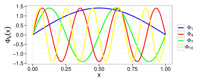
(a)

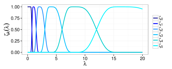
(b)

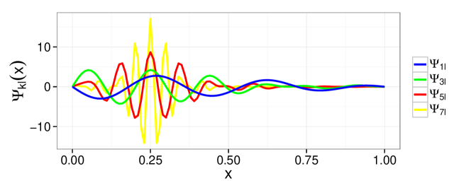
(c)

Figure 1: Littlewood-Paley on $L^{2}(0,1)$: (a) eigenfunctions; (b) multiscale bandpass filter; (c) frame elements.

3 Construction and Properties

3.1 Construction of a tight graph frame

As discussed earlier, the principle of Laplacian Eigenmaps is to use the basis $(\Phi_{i})_{1\leq i\leq n}$ to represent and process the data. An important advantage of this basis as compared with the natural basis of $\mathbb{R}^{d}$ is that it will be adapted to the geometry of the underlying submanifold $\mathcal{M}$ supporting the data distribution. For instance, in the denoising problem, a reasonable estimator of $f$ could be a truncated expansion of the noisy vector of observations $Y$ in the basis $(\Phi_{i})_{1\leq i\leq n}$.

On the other hand, a disadvantage of this basis is that it is not spatially localized. To get an intuitive view, consider the simple case of the interval $[0,1]$ with uniformly distributed data. In the population view, the eigenbasis of the Laplacian is the Fourier basis. While a truncated expansion in this basis is well-adapted to represent functions that are uniformly regular, it is not well-suited for functions exhibiting locally varying regularity (as an extreme example, a signal that is very smooth everywhere except at a few singular points where it is discontinuous). By contrast, wavelet bases, because they are localized both in space and frequency, allow for an efficient (i.e. sparse) representation of signals with locally varying regularity.

If we now think of data supported on a one-dimensional submanifold (curve) of $\mathbb{R}^{d}$, we can expect that the Laplacian eigenmaps method will discover a warped Fourier basis following the curve; and, for a more general submanifold $\mathcal{M}$, “harmonics” on $\mathcal{M}$.

In order to go from this basis to a spatially localized dictionary, following ideas of gerard and Hammond11 , we use the principle of the Littlewood-Paley decomposition.

Let $G$ be an undirected geometric neighborhood graph with adjacency matrix $A$ constructed from $\mathfrak{D}$, and $L$ be an associated symmetric graph Laplace operator with increasing eigenvalues $0=\lambda_{1}\leq\lambda_{2}\leq\ldots\leq\lambda_{n}$ and normalized eigenvectors $\Phi_{i}\in\mathbb{R}^{n},i=1..n$.

We first define a set of vectors using a decomposition of unity and a splitting operation and we will show that this vector set is a Parseval frame.

Definition 2

Let $\{\zeta_{k}\}_{k\in\mathbb{N}}$ be a sequence of functions $\zeta_{k}:\mathbb{R}_{+}\rightarrow[0,1]$ satisfying

(DoU)

$~{}~{}\sum_{j\geq 0}\zeta_{j}(x)=1$ for all $x\geq 0$;

(FD)

$~{}~{}\#\{\zeta_{k}:\zeta_{k}(\lambda_{i})\neq 0\}<\infty$ for $i=1,\ldots,n$.

Then we define the set of column vectors $\{\Psi_{kl}\in\mathbb{R}^{n},0\leq k\leq Q,1\leq j\leq n\}$ by

$$\Psi_{kl}=\sum_{i=1}^{n}\sqrt{\zeta_{k}(\lambda_{i})}\Phi_{i}(x_{l})\Phi_{i}.$$ (8)

with $Q:=\max\{k:\exists i\in\left\{1,\ldots,n\right\}\text{ with }\zeta_{k}(\lambda_{i})>0\}$.

Theorem 3.1

$\{\Psi_{kl}\}_{k,l}$ is a Parseval frame for $\mathcal{H}=\mathbb{R}^{n}$, that is for all $x\in\mathbb{R}^{n}$:

$$\sum_{k,l}\left\lvert\left\langle x,\Psi_{kl}\right\rangle\right\rvert^{2}=\left\lVert x\right\rVert^{2}\,.$$ (9)

Proof

If we can show that $\sum_{(k,l)}\Psi_{kl}\Psi_{kl}^{t}=\mathbf{I}_{n}$, we get immediately

$$y=\mathbf{I}_{n}y=\left(\sum_{(k,l)}\Psi_{kl}\Psi_{kl}^{t}\right)y\stackrel{{\scriptstyle}}{{=}}\sum_{(k,l)}\left\langle y,\Psi_{kl}\right\rangle\Psi_{kl},$$ (10)

for $y\in\mathbb{R}^{n}$. According to theorem 2.1 this equation is equivalent to the condition (1) with $A=B=1$. So we are done. It remains to show $\sum_{k,l}\Psi_{kl}\Psi_{kl}^{t}=\mathbf{I}_{n}$. We have (since we sum over a finite number of elements)

$$\sum_{(k,l)}\Psi_{kl}\Psi_{kl}^{t} = \sum_{k,l,i,j}\sqrt{\zeta_{k}(\lambda_{i})}\sqrt{\zeta_{k}(\lambda_{j})}\Phi_{i}(x_{l})\Phi_{j}(x_{l})\Phi_{i}\Phi_{j}^{t}$$ (11)

$$= \sum_{i=1}^{n}\sum_{k=0}^{Q}\zeta_{k}(\lambda_{i})\,\Phi_{i}\Phi_{i}^{t}$$

$$= \sum_{i=1}^{n}\Phi_{i}\Phi_{i}^{t}=\mathbf{I}_{n}.$$

For the second equality, we have used that $\sum_{l}\Phi_{i}(x_{l})\Phi_{j}(x_{l})=\left\langle\Phi_{i},\Phi_{j}\right\rangle={\mathbf{1}\{i=j\}}$, since $\{\Phi_{i}\}_{i}$ is an orthonormal basis (onb). For the third equality, we used (DoU), and for the last again the onb property. ∎

We now choose a special sequence of functions satisfying the decomposition of unity (DoU) condition while also ensuring (a) a spectral localization property for the frame elements and (b) a multiscale decomposition interpretation of the resulting decomposition. This construction follows gerard , and is known in the context of functional analysis as a smooth Littlewood-Paley decomposition.

Definition 3 (Multiscale bandpass filter)

Let $g\in C^{\infty}(\mathbb{R}_{+})$, $\mathop{\mathrm{supp}}g\subset[0,1]$, $0\leq g\leq 1$, $g(u)=1$ for $u\in[0,1/b]$ (for some constant $b>1$). For $k\in\mathbb{N}=\{0,1,\ldots\}$ the functions $\zeta_{k}:\mathbb{R}_{+}\rightarrow[0,1]$ are defined by

$$\zeta_{k}(x):=\begin{cases}g(x)&\text{if }k=0\\ g(b^{-k}x)-g(b^{-k+1}x)&\text{if }k>0\\ \end{cases}$$ (12)

The sequence $\{\zeta_{k}\}_{k\geq 0}$ is called multiscale bandpass filter.

This definition leads to the following properties: $\zeta_{k}(x)=\zeta_{1}(b^{-k}x)$ for $k\geq 1$ (multiscale decomposition), $\zeta_{k}\in C^{\infty}(\mathbb{R}_{+})$, $0\leq\zeta_{k}\leq 1$, $\mathop{\mathrm{supp}}\zeta_{0}\subset[0,1]$, $\mathop{\mathrm{supp}}\zeta_{k}\subset[b^{k-2},b^{k}]$ for $k\geq 1$ (spectral localization property). Moreover, one can check readily

$$\sum_{j\geq 0}\zeta_{j}(x)=1,$$ (13)

i.e., the (DoU) condition holds. In practice, we use a dyadic bandpass filter, that is, $b=2$. The functions $\zeta_{0},\ldots,\zeta_{5}$ with $b=2$ are displayed in Figure 1b. By construction, the parameter $k$ in $\Psi_{kl}$ is naturally a spectral scale parameter, while $l$ is a spatial localization parameter: the frame element $\Psi_{kl}$ is localized around the point $x_{l}$, as we discuss next.

3.2 Spatial localization

By construction, the elements of the frame are band-limited, i.e. localized in the spectral scale, in the sense that for a fixed $k$, the frame elements $\Psi_{kl}$ ($l=1,\ldots,n$) are linear combinations of the eigenvectors of the graph Laplacian (“graph harmonics”) corresponding to eigenvalues in the range $[b^{k-2},b^{k}]$ only.

From our initial motivations, it is desirable that in contrast with the eigenfunctions of the Laplace operator, the frame elements $\Psi_{kl}$ are spatially localized functions. In the classical Littlewood-Paley construction for the usual Laplacian on the interval $[0,1]$, this is a well-known fact: the use of linear combination of trigonometric functions $\Psi_{kl}(y):=\sin(kl)\sin(ky)$ via smooth multiscale bandpass filters weights as described in Definition 3 gives rise to strongly localized functions (as illustrated in Figure 1).

Regarding the corresponding discrete construction based on the graph Laplacian, this localization property is certainly observed in practice (as illustrated in Figure 2 and 3, see Section 4 for the setup of the numerical experiments).

Concerning the theoretical perspective, we first review briefly the existing results of Hammond11 , denote $d$ the shortest path distance in the graph. Theorem 5.5 of Hammond11 there gives the following localization result for graph frames:

$$\frac{\Psi_{kl}(x)}{\left\lVert\Psi_{kl}\right\rVert_{2}}\leq Cb^{-k}\,,$$ (14)

for all $x$ with $d(x,x_{l})\geq K$, under the assumption that the scaling function $\zeta_{1}$ is $K$-times differentiable with vanishing first $(K-1)$ derivatives in 0, non-vanishing $K$-th derivative, and the scale parameter $k$ is big enough. This says that $\Psi_{kl}$ is “localized” around the point $x_{l}$. Unfortunately, this result is not informative in our framework for two reasons: first, we chose a function $\zeta_{1}$ (see (12)) vanishing in a neighborhood of zero, so that all derivatives vanish in the origin, contradicting one of the above assumptions. Secondly, and independently of this first issue, the condition “$k$ is big enough”, as well as the factor $C$, depend on the size $n$ of the graph and of the largest eigenvalue of the Laplacian. As a consequence it is unclear if this bound covers any interesting part of the spectrum (for $k$ too large, the spectral support $[b^{k-2},b^{k}]$ does not contain any eigenvalues, so that $\Psi_{kl}$ is trivial). Finally, for fixed $k$ the bound also does not give information on the behavior of $\Psi_{kl}(x)$ when the path distance of $x$ to $x_{l}$ becomes very large.

On the other hand the form of the scaling function $\zeta_{1}$ used in the present work is based on gerard where a theory of multiscale frame analysis is developed on very general metric spaces under certain geometrical assumptions. Without entering into detail, it is proved there that using this construction, the obtained frame functions $\Psi_{kl}(x)$ are upper bounded by $O((d(x,x_{l})/b^{k})^{-\nu})$ for $\nu$ arbitrary large. We observe that this type of localization estimate is sharper than (14) for fixed $x$ and growing $k$, as well as for fixed scale $k$ and varying $x$. We conjecture that these theoretical results apply meaningfully in the discrete setting considered here, under the assumption that $x_{1},\ldots,x_{n}$ are iid from a sufficiently regular distribution $\mathbf{P}_{0}$ on a regular manifold $\mathcal{M}$, but it is out of the intended scope of the present paper to establish this formally. In particular “meaningfully” means that the constants involved in the bounds should be independent of the graph size (otherwise the bounds could potentially be devoid of interest for any particular graph, as pointed out above), a question that we are currently investigating.

Figure 2: Swiss roll data: top: eigenvectors $\Phi_{j}$ for $j=10,30,50,100$; bottom: frame elements $\Psi_{kl}$ for $l$ fixed and $k=0,2,5,7$. (Construction from actual swiss roll data, then “unrolled” for clearer graphical representation.)

Figure 3: Sphere data: frame elements $\Psi_{kl}$ for $l$ fixed and $k=1,5,7$

4 Denoising

We consider the regression model for fixed design points $\mathfrak{D}=\left\{x_{i},i=1..n\right\}$ and observations $y_{i}=f(x_{i})+\epsilon_{i}$ ($\epsilon_{i}$ are independent and identically distributed random variables with $\mathbf{E}\left(\epsilon_{i}\right)=0$ and $\mathbf{Var}\left(\varepsilon\right)_{i}=\sigma^{2}$). The aim of denoising is to recover the function $f:\mathfrak{D}\rightarrow\mathbb{R}$ at the design points themselves. We will use the proposed Parseval frame in order to define an estimate ${\widehat{f}}$ of the function $f$. In what follows, since the $\mathfrak{D}$ is fixed, we identify $f$ with the vector $(f(x_{1}),\ldots,f(x_{n}))$ and denote $y=(y_{1},\ldots,y_{n})$.

Given the frame $\mathcal{F}$ with a multiscale bandpass filter as defined in 2 and 3 associated to the data points $\mathfrak{D}$, we denote the frame coefficients $a_{kl}=\left\langle\Psi_{kl},f\right\rangle$ for $f$ and $b_{kl}=\left\langle\Psi_{kl},y\right\rangle$ for $y$. Due to the linearity of the inner product we get $a_{kl}=b_{kl}-\left\langle\Psi_{kl},\epsilon\right\rangle.$ We estimate the unknown coefficients $a_{kl}$ by adjusting the known coefficients $b_{kl}$ by soft-thresholding:

$$S_{s}\left(z,c\right)=\mathop{\mathrm{sgn}}(z)\,(\left\lvert z\right\rvert-c)_{+}.$$ (15)

In order to take into account that the frame elements $\Psi_{kl}$ are not normalized, and generally have different norms, we use element-adapted thresholds of the form $c_{kl}=\sigma\left\lVert\Psi_{kl}\right\rVert t$ which depend on the variance of $\left\langle\epsilon,\Psi_{kl}\right\rangle$ and some global parameter $t$. Equivalently, this corresponds to first normalizing the observed coefficients $b_{kl}$ by dividing by their variance, then applying a global threshold to the normalized coefficients, and finally inverting the normalization.

The estimator of $f$ is then the plug-in estimator

$${\widehat{f}}_{S}=\sum_{k,l}S\left(b_{kl},c_{kl}\right)\Psi_{kl}=T^{*}S(b,c),$$ (16)

where $S(b,c)$ denotes the vector of thresholded coefficients, and $T^{*}$ is the synthesis operator of the frame as introduced in Section 2.2.

To measure the performance of this estimator, we use the risk measure

$$Risk({\widehat{f}},f)=\mathbf{E}_{\epsilon}\left(\left\lVert{\widehat{f}}-f\right\rVert^{2}\right),$$ (17)

that is, the expected quadratic norm at the sampled points (where $\left\lVert f\right\rVert^{2}=\sum_{i=1}^{n}f(x_{i})^{2}$ is the Euclidean vector norm of $f$ on the observation points), for the performance analysis of an estimator ${\widehat{f}}\in\mathbb{R}^{n}$.

For bounding the risk of the thresholding estimator ${\widehat{f}}_{S}$, rather than assuming some specific regularity properties on the function $f$, it is useful to compare the performance of ${\widehat{f}}_{S}$ to that of a group of reference estimators. This is called the oracle approach Candes06 ; Donoho94 : can the proposed estimator have a performance (almost) as good as the best estimator (for this specific $f$) in a reference family (that is to say, as good as if an oracle would have given us advance knowledge of which reference estimator is the best for this function $f$). We review here briefly some important results.

A suitable class of simple reference estimators consists of “keep or kill” (or diagonal projection) estimators, that keep without changes the observed coefficients $b_{k,l}$ for $(k,l)$ in some subset $I$, and put to zero the coefficients for indices outside of $I$:

$${\widehat{f}}_{I}:=\sum_{(k,l)\in I}b_{kl}\Psi_{kl}=T^{*}{\widehat{a}}^{I}_{kl},$$ (18)

where ${\widehat{a}}^{I}_{kl}=b_{kl}{\mathbf{1}\{(k,l)\in I\}}$. Now using the frame reconstruction formula and (6), we obtain

$$\mathbf{E}_{\epsilon}\left(\left\lVert{\widehat{f}}_{I}-f\right\rVert^{2}\right) = \mathbf{E}_{\epsilon}\left(\left\lVert T^{*}(a-{\widehat{a}}^{I})\right\rVert^{2}\right)$$ (19)

$$\leq \mathbf{E}_{\epsilon}\left(\left\lVert a-{\widehat{a}}^{I}\right\rVert^{2}\right)$$

$$= \sum_{(k,l)}\big{(}a_{kl}^{2}{\mathbf{1}\{(k,l)\not\in I\}}$$

$$\;\;\;+\sigma^{2}\left\lVert\psi_{kl}\right\rVert^{2}{\mathbf{1}\{(k,l)\in I\}}\big{)}\,.$$

Therefore, the optimal (oracle) choice of the index set $I^{*}$ obtained by minimizing the above upper bound is given by

$$(k,l)\in I^{*}~{}~{} \Leftrightarrow~{}~{}\left\langle f,\Psi_{kl}\right\rangle^{2}\geq\sigma^{2}\left\lVert\Psi_{kl}\right\rVert^{2}~{}\mbox{~{}~{}(keep)~{}~{}}$$ (20)

$$(k,l)\notin I^{*}~{}~{} \Leftrightarrow~{}~{}\left\langle f,\Psi_{kl}\right\rangle^{2}\leq\sigma^{2}\left\lVert\Psi_{kl}\right\rVert^{2}~{}\mbox{~{}~{}(kill)~{}~{}}.$$

One deduces from this that

$$\inf_{I}\mathbf{E}_{\epsilon}\left(\left\lVert{\widehat{f}}_{I}-f\right\rVert^{2}\right)\leq\sum_{(k,l)\in N}\min\left(\left\langle f,\Psi_{kl}\right\rangle^{2},\sigma^{2}\left\lVert\Psi_{kl}\right\rVert^{2}\right)=:OB(f)\,.$$ (21)

The relation of soft thresholding estimators to the collection of keep-or-kill estimators on a Parseval frame is captured by the following oracle-type inequality (see Candes06 , Section 9):

Theorem 4.1

Let $\{\Psi_{kl}\}_{k,l}$ be a Parseval frame and consider the denoising observation model. Let ${\widehat{f}}_{S_{s}}=\sum_{k,l}S_{s}\left(\left\langle y,\Psi_{kl}\right\rangle,t_{kl}\right)\Psi_{kl}$ be the soft-threshold frame estimator from (16). Then with $t_{kl}=\sigma\left\lVert\Psi_{kl}\right\rVert\sqrt{2\log(n)}$ the following inequality holds:

$$\mathbf{E}_{\epsilon}\left(\left\lVert{\widehat{f}}_{S_{s}}-f\right\rVert^{2}\right)\leq\left(2\log(n)+1\right)\left(\sigma^{2}+OB(f)\right).$$ (22)

To interpret this result, observe that if we renormalize the squared norm by $\frac{1}{n}$, so that it represents averaged squared error per point, we expect (depending on the regularity of $f$) the order of magnitude of $n^{-1}OB(f)$ to be typically a polynomial rate $O(n^{-\nu})$ for some $\nu<1$. Then the term $\sigma^{2}/n$ is negligible in comparison, and the oracle inequality states that the performance of ${\widehat{f}}_{S_{s}}$ is only worse by a logarithmic factor than the performance obtained with the optimal, $f$-dependent choice of $I$ in a keep-or-kill estimator.

For this tight oracle inequality to hold, it is particularly important that a Parseval frame is used. While thresholding strategies can also be applied to the coefficients of a frame that is not Parseval, the reconstruction step is less straightforward, (the canonical dual frame must be computed for reconstruction from the thresholded coefficients, see Section 2.2); furthermore, an additional factor $B/A$ comes into the bound ($A\leq 1\leq B$ being the frame bounds from definition (1)) (see for instance, Haltmeier12 , Prop. 3.10). Therefore, the performance of simple thresholding estimates deteriorates when used with a non-Parseval frame.

5 Numerical experiments

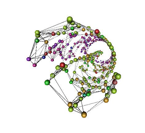
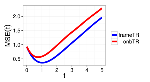
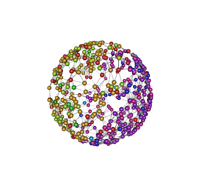
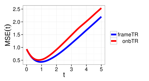
Figure 4: Left: noisy function on swiss roll data (top) and sphere data (bottom), graph representation. Right: MSE for two representative settings (weighted $\varepsilon$-Graph and $k$-NN-Graph) as a function of threshold level. Red is thresholding in the original Laplacian Eigenmaps ONB, blue is thresholding of frame coefficients.

Table 1: MSE performance under optimal parameter choice. FrTh = Frame Tresholding; LETh/LETr = Laplacian Eigenmaps Thresholding/Truncated expansion. Prefix W indicates edge weighting in the graph. CGK is the complete graph with Gaussian weights. U/N is un/normalized graph Laplacian.Standard error in brackets.Top: Sphere example. Bottom: swiss roll example

Example: sphere, jump function,$\sigma^{2}=1,n=500,m=50$ Graph $L$ FrTh LETh LETr kNN U 0.510   (0.050) 0.693   (0.061) 0.905   (0.108) kNN N 0.538   (0.046) 0.712   (0.055) 0.931   (0.094) WkNN U 0.521   (0.049) 0.652   (0.050) 0.800   (0.097) WkNN N 0.530   (0.049) 0.674   (0.057) 0.749   (0.091) CGK U 0.520   (0.055) 0.638   (0.065) 0.821   (0.107) CGK N 0.530   (0.052) 0.670   (0.050) 0.725   (0.081) $\epsilon$G U 0.505   (0.058) 0.650   (0.068) 0.865   (0.115) $\epsilon$G N 0.557   (0.052) 0.710   (0.059) 0.902   (0.106) W$\epsilon$G U 0.482   (0.055) 0.622   (0.064) 0.787   (0.111) W$\epsilon$G N 0.530   (0.049) 0.674   (0.057) 0.749   (0.091)

Smoothing Kernel Regression: min. MSE = 0.612 (0.066)

Kernel Ridge Regression: min. MSE = 0.594 (0.051)

Example: swiss roll, jump function,$\sigma^{2}=1,n=500,m=50$ Graph $L$ FrTh LETh LETr kNN U 0.462   (0.043) 0.647   (0.039) 0.876   (0.079) kNN N 0.494   (0.043) 0.676   (0.043) 0.902   (0.071) WkNN U 0.443   (0.045) 0.600   (0.050) 0.790   (0.102) WkNN N 0.500   (0.043) 0.659   (0.045) 0.775   (0.079) CGK U 0.491   (0.053) 0.625   (0.057) 0.844   (0.096) CGK N 0.520   (0.047) 0.648   (0.049) 0.713   (0.079) $\epsilon$G U 0.459   (0.049) 0.610   (0.053) 0.872   (0.095) $\epsilon$G N 0.532   (0.045) 0.681   (0.050) 0.884   (0.089) W$\epsilon$G U 0.441  (0.049) 0.574   (0.049) 0.793   (0.113) W$\epsilon$G N 0.503   (0.045) 0.643   (0.051) 0.744   (0.089)

Smoothing Kernel Regression: min. MSE = 0.589 (0.082)

Kernel Ridge Regression: min. MSE = 0.779 (0.052)

We investigate the performance of the proposed method for denoising on two testbed datasets where the ground truth is known and the design points are drawn randomly iid from a distribution on a manifold. More precisely, we will consider one example where the design points $\mathfrak{D}$ are drawn uniformly ($n=500$) on the unit square, which is then rolled up into a “swiss roll” shape in 3D. We consider a very simple target function represented (on the original unit square) as a piecewise constant function (with values 5 and -3) on two triangles, displaying a sharp discontinuity along one diagonal of the square and very smooth regularity elsewhere. This function is observed with an additional Gaussian noise of variance $\sigma^{2}=1$. In the second example the design points $\mathfrak{D}$ are drawn uniformly ($n=500$) on the unit sphere in $\mathbb{R}^{3}$. The target function remains a piecewise constant function, defined on the two parts of the sphere when intersecting it with a chosen plane. Again, this function is observed with an additional Gaussian noise of variance $\sigma^{2}=1$. For the swiss roll example as well as for the sphere example, one sample consisting of design points and noisy function values is displayed in Figure 4.

In each example, we consider the different types of neighborhood graphs described in Section 2.3. Following usual heuristics, for the construction of the $k$-NN graph we take $k=7\approx\log n$; for the $\varepsilon$-graph, we take for $\varepsilon$ the average distance to the $k=7$th nearest neighbor, and for weighted graphs we take Gaussian weights, where the bandwidth $\lambda$ is calibrated so that points at the distance $\varepsilon$ defined above are given weight $0.5$.

After constructing the (weighted or unweighted) graph Laplacian, we compute explicitly its eigendecomposition. For the construction of the frame via the multiscale bandpass filter, we use a ${\mathcal{C}}^{3}$ piecewise polynomial plateau function $g$ satisfying the support constraints of Definition 3 for $b=2$ (i.e. constant equal to 1 for $x\leq 0.5$, and zero for $x\geq 1$). While this function is not ${\mathcal{C}}^{\infty}$, it has the advantage of fast computation.

We compare the denoising performance of the following competitors: Parseval frame with soft thresholding, soft thresholding applied to the Laplacian Eigenmaps orthormal basis, and truncated expansion in the Laplacian Eigenmaps basis (only the $k$ coefficients corresponding to the first eigenvalues are kept, without thresholding). The latter method is in the spirit of LapEig2 . It is well-known (from the regular grid case) that the “universal” theoretical threshold $\sigma\sqrt{\log n}$ is often too conservative in practice. For a fair comparison, we therefore compute the mean squared error (MSE) of both thresholding methods for varying threshold $t$ (still modulated by $\left\lVert\Psi_{kl}\right\rVert$ for the Parseval frame). Comparison of the MSE for one sample accross the $t$-range for two particular settings is plotted on Figure 4. For all studied settings (different graph and graph Laplacian types), for the same threshold level $t$ we observed that the frame-based method systematically shows a noticeable improvement.

In Table 1 we report the minimum MSEs and their standard error (averaged over $m=50$ samples of design points and independent noise) for different methods over the possible range of the parameter (threshold level $t$, resp. number of coefficients for truncated expansion), both for the swissroll and for the sphere example. We observe an improvement of 20 to 25% across the different settings (the best overall results being obtained with weighted graphs and the unnormalized Laplacian). We also compared to the more traditional methods of kernel smoothing (Nadaraya-Watson estimator) and kernel ridge regression, using a Gaussian kernel (also with optimal choices of bandwidth and regularization parameter), and observed a comparable performance improvement. While it is not realistic to assume that the optimal parameter choice is known in practice, it is fair to compare all methods under their respective optimal parameter settings, as parameter selection methods will induce a comparable performance hit with respect to the best setting.

6 Outlook

Following the recently introduced idea of generalizing the Littlewood-Paley spectral decomposition, we constructed explicitly a Parseval frame of functions on a neighborhood graph formed on the data points. We established that a thresholding strategy on the frame coefficients has superior performance for the denoising problem as compared to usual, spectral or non-spectral, approaches. Future developments include extension of this methodology to the semisupervised learning setting, and a stronger theoretical basis for spatial localization.

Appendix

7 Proof of Theorem 3

Theorem 4.1 states a oracle-type inequality which captures the relation of soft thresholding estimators $\hat{f}_{S_{s}}=\sum_{k,l}S_{s}\left(\left\langle y,\Psi_{kl}\right\rangle,t_{kl}\right)\Psi_{kl}$ defined in (16) to the collection of keep-or-kill estimators on a Parseval frame. This result is known in the literature (see Candes06 , Section 9), but we provide a short self-contained proof for completeness, modulo a technical result from Donoho94 for soft thresholding of a single one-dimensional Gaussian variable, which is basic for the proof of theorem 4.1.

Lemma 1

For $0\leq\delta\leq 1/2$, $t=\sqrt{2\log(\delta^{-1})}$ and $X\sim\mathcal{N}(\mu,1)$

$$\mathbf{E}_{X}\left(\left(S_{s}(X,t)-\mu\right)^{2}\right) \leq (2\log(\delta^{-1})+1)(\delta+\min(1,\mu^{2}))$$ (23)

$$= (t^{2}+1)\left(\exp\left(-\frac{t^{2}}{2}\right)+\min(1,\mu^{2})\right).$$

The proof of this lemma can be found in appendix 1 of Donoho94 . Now we are able to prove theorem 4.1.

Proof

First note that for $y=\tau x,\tau>0$, we have

$$S_{s}(y,u)=\tau S_{s}\left(x,\frac{u}{\tau}\right).$$ (24)

Secondly we remark that

$$\frac{\left\langle y,\Psi_{kl}\right\rangle}{\sigma\left\lVert\Psi_{kl}\right\rVert}\sim\mathcal{N}\left(\frac{a_{kl}}{\sigma\left\lVert\Psi_{kl}\right\rVert},1\right).$$ (25)

Considering now the risk of the soft thresholding estimator $\hat{f}_{S_{s}}$ we get

$$\mathbf{E}\left(\left\lVert\hat{f}_{S_{s}}-f\right\rVert^{2}\right) = \mathbf{E}\left(\left\lVert\sum_{k,l}\left(S\left(\left\langle y,\Psi_{kl}\right\rangle,t_{kl}\right)-a_{kl}\right)\Psi_{kl}\right\rVert^{2}\right)$$ (26)

$$\leq \mathbf{E}\left(\sum_{k,l}\left(S\left(\left\langle y,\Psi_{kl}\right\rangle,t_{kl}\right)-a_{kl}\right)^{2}\right)$$

$$= \sum_{k,l}\mathbf{E}\left(\left(S\left(\left\langle y,\Psi_{kl}\right\rangle,t_{kl}\right)-a_{kl}\right)^{2}\right).$$

by using inequality (6). By applying (24) and then (23) with $t=\sqrt{2\log(n)}$ it follows that

$$\mathbf{E}\left(\left\lVert\hat{f}_{S_{s}}-f\right\rVert^{2}\right)\leq\sum_{k,l}\sigma^{2}\left\lVert\Psi_{kl}\right\rVert^{2}\mathbf{E}\left(\left(S\left(\frac{\left\langle y,\Psi_{kl}\right\rangle}{\sigma\left\lVert\Psi_{kl}\right\rVert},\sqrt{2\log(n)}\right)-\frac{a_{kl}}{\sigma\left\lVert\Psi_{kl}\right\rVert}\right)^{2}\right)$$ (27)

$$\leq \sum_{k,l}\sigma^{2}\left\lVert\Psi_{kl}\right\rVert^{2}(2\log(n)+1)\left(\exp\left(-\frac{2\log(n)}{2}\right)+\min\left(1,\frac{a_{kl}^{2}}{\sigma^{2}\left\lVert\Psi_{kl}\right\rVert^{2}}\right)\right)$$

$$= \sum_{k,l}(2\log(n)+1)\left(\frac{1}{n}\sigma^{2}\left\lVert\Psi_{kl}\right\rVert^{2}+\min\left(\sigma^{2}\left\lVert\Psi_{kl}\right\rVert^{2},a_{kl}^{2}\right)\right)$$

$$= (2\log(n)+1)\left(\frac{1}{n}\sum_{k,l}\sigma^{2}\left\lVert\Psi_{kl}\right\rVert^{2}+\sum_{k,l}\min\left(\sigma^{2}\left\lVert\Psi_{kl}\right\rVert^{2},a_{kl}^{2}\right)\right).$$

Recalling the Parseval frame property $\sum_{k,l}\left\lVert\Psi_{kl}\right\rVert^{2}=n$, we finally obtain

$$\mathbf{E}\left(\left\lVert\hat{f}_{S_{s}}-f\right\rVert^{2}\right) \leq (2\log(n)+1)\left(\frac{1}{n}n\sigma^{2}+\sum_{k,l}\min\left(\sigma^{2}\left\lVert\Psi_{kl}\right\rVert^{2},a_{kl}^{2}\right)\right)$$ (28)

$$= (2\log(n)+1)\left(\sigma^{2}+\sum_{k,l}\min\left(\sigma^{2}\left\lVert\Psi_{kl}\right\rVert^{2},a_{kl}^{2}\right)\right).$$

where we recognize the upper bound $\sum_{k,l}\min\left(\sigma^{2}\left\lVert\Psi_{kl}\right\rVert^{2},a_{kl}^{2}\right)=OB(f)$ for the oracle. ∎

References

- (1) Belkin, M., Niyogi, P.: Using manifold stucture for partially labeled classification. In: NIPS, pp. 929–936 (2002)
- (2) Belkin, M., Niyogi, P.: Laplacian eigenmaps for dimensionality reduction and data representation. Neural Computation 15(6), 1373–1396 (2003)
- (3) Bickel, P., Li, B.: Complex datasets and inverse problems: tomography, networks and beyond, vol. 54, chap. Local Polynomial Regression on Unknown Manifolds, pp. 177–186. IMS lecture Notes (2007)
- (4) Cand s, E.: Modern statistical estimation via oracle inequalities. Acta Numerica 15, 257–325 (2006)
- (5) Casazza, P., Kutyniok G.and Philipp, F.: Introduction to finite frame theory. In: P.G. Casazza, G. Kutyniok (eds.) Finite Frames, Applied and Numerical Harmonic Analysis, pp. 1–53. Birkh user Boston (2013)
- (6) Christensen, O.: Frames and Bases: An Introductory Course (Applied and Numerical Harmonic Analysis). Birkh user (2008)
- (7) Coulhon, T., Kerkyacharian, G., Petrushev, P.: Heat kernel generated frames in the setting of Dirichlet spaces. J. Fourier Anal. Appl. 18(5), 995–1066 (2012)
- (8) Donoho, D.L., Johnstone, I.M.: Ideal spatial adaptation by wavelet shrinkage. Biometrika 81(3), 425–455 (1994)
- (9) Gavish, M., Nadler, B., Coifman, R.R.: Multiscale wavelets on trees, graphs and high dimensional data: Theory and applications to semi supervised learning. In: J. F rnkranz, T. Joachims (eds.) ICML, pp. 367–374. Omnipress (2010)
- (10) Haltmeier, M., Munk, A.: Extreme Value Analysis of Empirical Frame Coefficients and Implications for Denoising by Soft-Thresholding. ArXiv e-print (2012). To appear in Applied and Computational Harmonic Analysis
- (11) Hammond, D.K., Vandergheynst, P., Gribonval, R.: Wavelets on graphs via spectral graph theory. Applied and Computational Harmonic Analysis 30(2), 129 – 150 (2011)
- (12) Han, D.: Frames for Undergraduates. Student mathematical library. American Mathematical Society (2007)
- (13) Kpotufe, S.: k-NN regression adapts to local intrinsic dimension. In: NIPS, pp. 729–737 (2011)
- (14) Kpotufe, S., Dasgupta, S.: A tree-based regressor that adapts to intrinsic dimension. J. Comput. Syst. Sci. 78(5), 1496–1515 (2012)
- (15) Roweis, S., Saul, L.: Nonlinear dimensionality reduction by locally linear embedding. Science 290, 2323–2326 (2000)
- (16) Tenenbaum, J., de Silva, V., Langford, J.: A global geometric framework for nonlinear dimensionality reduction. Science 290, 2319–2323 (2000)