Convergence of Finite Difference schemes for
the Benjamin–Ono equation

Abstract.

In this paper, we analyze finite difference schemes for Benjamin–Ono equation, $u_{t}=uu_{x}+Hu_{xx}$, where $H$ denotes the Hilbert transform. Both the decaying case on the full line and the periodic case are considered. If the initial data are sufficiently regular, fully discrete finite difference schemes shown to converge to a classical solution. Finally, the convergence is illustrated by several examples.

1. Introduction

This paper considers a fully discrete finite difference scheme for the Benjamin–Ono (BO) equation. The BO equation models the evolution of weakly nonlinear internal long waves. It has been derived by Benjamin [2] and Ono [12] as an approximate model for long-crested unidirectional waves at the interface of a two-layer system of incompressible inviscid fluids, one being infinitely deep. In non-dimensional variables, the initial value problem associated with the BO equation reads

(1.1) $$\begin{cases}u_{t}=uu_{x}+Hu_{xx},\quad x\in\mathbb{R},\ 0\leq t\leq T,&\\ u|_{t=0}=u_{0},&\end{cases}$$

where $H$ denotes the Hilbert transform defined by the principle value integral

$$Hu(x):=\mathrm{P.V.}\,\frac{1}{\pi}\int_{\mathbb{R}}\frac{u(x-y)}{y}\,dy.$$

The BO equation is, at least formally, completely integrable [1] and thus possesses an infinite number of conservation laws. For example, the momentum and the energy, given by

$$M(u):=\int u^{2}\,dx,\,\,\text{and}\,\,E(u):=\frac{1}{2}\int\left|D_{x}^{1/2}u\right|^{2}\,dx+\frac{1}{6}\int u^{3}\,dx,$$

are conserved quantities for solutions of (1.1).

We also consider the corresponding $2L$-periodic problem

(1.2) $$\begin{cases}u_{t}=uu_{x}+\mathbb{H}_{\rm per}u_{xx},\quad&x\in\mathbb{T},\ 0\leq t\leq T,\\ u|_{t=0}=u_{0},&x\in\mathbb{T}\end{cases}$$

where $\mathbb{T}:=\mathbb{R}/2L\mathbb{Z}$. The periodic Hilbert transform is defined by the principle value integral

$$\mathbb{H}_{\rm per}u(x)=\mathrm{P.V.}\frac{1}{2L}\int_{-L}^{L}\cot\Bigl{(}\frac{\pi}{2L}y\Bigr{)}u(x-y)\,dy.$$

The initial value problem (1.1) has been extensively studied in recent years. Well-posedness of (1.1) in $H^{s}(\mathbb{R})$, for $s>3$ was proved by Iorio [9] using purely hyperbolic energy methods. Then, Ponce [15] derived a local smoothing effect associated to the dispersive part of the equation, which combined with compactness methods, enabled him to prove well-posedness also for $s=3$.

By combining a complex version of the Cole–Hopf transform with Strichartz estimates, Tao [18] was able to show well-posedness of the Cauchy problem (1.1) in $H^{1}(\mathbb{R})$. This well-posedness was extended to $H^{s}(\mathbb{R})$ for $s>1$ by Burq and Planchon [4] and for $s\geq 0$ by Ionescu and Kenig [8]. In the periodic setting, Molinet [11] proved well-posedness in $H^{s}(\mathbb{T})$ for $s\geq 0$. For operator splitting methods applied to the BO equation, see [6].

In this paper, we define a numerical scheme for both (1.1) and (1.2), with the aim to develop a convergent finite difference scheme. While there are several numerical methods for the BO equation which perform well in practice, indeed better than the one presented here, see [3] for a recent comparison of different numerical methods, we emphasize that we here prove the convergence of our proposed scheme. Having said this, there are results concerning error estimates for the BO equation in [19, 14, 5]. However, error estimate analysis a priori assumes existence of solutions of the underlying equation, while our convergence analysis, as a by-product, can be viewed as a constructive proof for the existence of solutions of the BO equation (1.1). It is worth mentioning that the scheme under consideration in this paper is similar to the scheme analyzed in [19], the only difference being that a different discretization of Hilbert transform is introduced in this paper.

We analyze the fully discrete Crank–Nicolson difference scheme

(1.3) $$u^{n+1}_{j}=u^{n}_{j}+{\Delta t}\,\tilde{u}^{n+1/2}_{j}Du^{n+1/2}_{j}+{\Delta t}\,\mathbb{H}\left(D_{+}D_{-}u^{n+1/2}\right)_{j},\quad n\in\mathbb{N}_{0},\,j\in\mathbb{Z},$$

where ${\Delta x},{\Delta t}$ are discretization parameters, $u^{n}_{j}\approx u(j{\Delta x},n{\Delta t})$ and $u^{n+1/2}=(u^{n}+u^{n+1})/2$. Furthermore, $D$ and $D_{\pm}$ denote symmetric and forward/backward (spatial) finite differences, respectively, $\mathbb{H}$ denotes a discrete Hilbert transform operator, and $\tilde{u}$ denotes a spatial average. We show (Theorem 2.9) that for initial data $u_{0}\in H^{2}(\mathbb{R})$ there exists a finite time $T$, depending only on the $H^{2}(\mathbb{R})$ norm of the initial data such that for $t\leq T$, the difference approximation (2.4) converges uniformly in $C(\mathbb{R}\times[0,T])$ to the unique solution of the BO equation (1.1) as ${\Delta x}\to 0$ with ${\Delta t}=\mathcal{O}({\Delta x})$. Furthermore, following [19, Theorem 3.2], a second-order error estimate in both time and space for smooth solutions can be obtained by our numerical method.

The rest of the paper is organized as follows: In Section 2, we present necessary notations to introduce the Crank–Nicolson scheme and present the convergence analysis in the full line case, in Section 3 we present the periodic Hilbert transform and outline the proofs in the periodic setting, and finally in Section 4, we test our numerical scheme and provide some numerical results.

2. The finite difference scheme

Throughout this paper, we use the letters $C$, $K$ etc. to denote various constants which may change from line to line. We start by introducing the necessary notation. Derivatives will be approximated by finite differences, and the basic quantities are as follows. For any function $p:\mathbb{R}\to\mathbb{R}$, we set

$$D_{\pm}p(x)=\pm\frac{1}{{\Delta x}}\big{(}p(x\pm{\Delta x})-p(x)\big{)},\ \text{and}\ D=\frac{1}{2}\left(D_{+}+D_{-}\right)$$

for some (small) positive number ${\Delta x}$. If we introduce the averages

$$\tilde{p}(x):=\frac{1}{3}\left(p(x+{\Delta x})+p(x)+p(x-{\Delta x})\right),\,\,\bar{p}(x):=\frac{1}{2}\left(p(x+{\Delta x})+p(x-{\Delta x})\right)$$

and the shift operator

$$S^{\pm}p(x)=p(x\pm{\Delta x}),$$

we find that

$$D(pq) =\bar{p}Dq+\bar{q}Dp,$$

$$D_{\pm}(pq) =S^{\pm}pD_{\pm}q+qD_{\pm}p=S^{\pm}qD_{\pm}p+pD_{\pm}q.$$

We discretize the real axis using ${\Delta x}$ and set $x_{j}=j{\Delta x}$ for $j\in\mathbb{Z}$. For a given function $p$, we define $p_{j}=p(x_{j})$. We will consider functions in $\ell^{2}$ with the usual inner product and norm

$$\langle p,q\rangle={\Delta x}\sum_{j\in\mathbb{Z}}p_{j}q_{j},\quad\left\|p\right\|=\left\|p\right\|_{2}=\langle p,p\rangle^{1/2},\qquad p,q\in\ell^{2}.$$

Moreover, we define $h^{2}$-norm of a grid function as

$$\left\|p\right\|_{h^{2}}:=\Bigl{(}\left\|p\right\|^{2}+\left\|D_{+}p\right\|^{2}+\left\|D_{+}D_{-}p\right\|^{2}\Bigr{)}^{1/2}.$$

Observe that

$$\left\|p\right\|_{\infty}:=\sup_{j\in\mathbb{Z}}\left|p_{j}\right|\leq\frac{1}{{\Delta x}^{1/2}}\left\|p\right\|.$$

In the periodic case, let $N$ be a given odd natural number. We divide the periodicity interval $[-L,L]$ into $N$ sub-intervals $[x_{j},x_{j+1}]$ using ${\Delta x}=\frac{2L}{N}$, where

$$x_{j}=-L+j{\Delta x},\quad\text{for}\quad j=0,1,2,.....,N.$$

In the periodic case the sum over $\mathbb{Z}$ is replaced by a finite sum $j=0,\dots,N$. The various difference operators enjoy the following properties:

$$\langle p,D_{\pm}q\rangle=-\langle D_{\mp}p,q\rangle,\quad\langle p,Dq\rangle=-\langle Dp,q\rangle,\qquad p,q\in\ell^{2}.$$

Furthermore, using Leibniz rules, the following identities can be readily verified:

(2.1a) $$\langle D(pq),q\rangle =\frac{{\Delta x}}{2}\langle D_{+}p\,Dq,q\rangle+\frac{1}{2}\langle S^{-}q\,Dp,q\rangle,$$

(2.1b) $$D_{+}D_{-}(pq) =D_{-}pD_{+}q+D_{+}D_{-}qS^{-}p+D_{+}pD_{+}q+qD_{+}D_{-}p.$$

We also need to discretize in the time direction. Introduce (a small) time step ${\Delta t}>0$, and use the notation

$$D^{t}_{+}p(t)=\frac{1}{{\Delta t}}\big{(}p(t+{\Delta t})-p(t)\big{)},$$

for any function $p\colon[0,T]\to\mathbb{R}$. Write $t_{n}=n{\Delta t}$ for $n\in\mathbb{N}_{0}=\mathbb{N}\cup\{0\}$. A fully discrete grid function is a function $u_{\Delta x}\colon{\Delta t}\,\mathbb{N}_{0}\to\mathbb{R}^{\mathbb{Z}}$, and we write $u_{\Delta x}(x_{j},t_{n})=u^{n}_{j}$. (A CFL-condition will enforce a relationship between ${\Delta x}$ and ${\Delta t}$, and hence we only use ${\Delta x}$ in the notation.)

Next we present a lemma, which essentially gives a relation between discrete and continuous Sobolev norms. Since we shall use this lemma frequently, for the sake of completeness, we present a proof of this lemma in the full line case.

Lemma 2.1.

There exists a constant $C$ such that for all $u\in H^{2}(\mathbb{R})$

$$\left\|u_{\Delta x}\right\|_{h^{2}}\leq C\,\left\|u\right\|_{H^{2}},$$

where we identify $u_{\Delta x}$ with the discrete evaluation $\left\{u(x_{j})\right\}_{j}$.

Proof.

To begin with, observe that the discrete operator $D_{+}D_{-}$ commutes with the continuous operator $\partial_{x}$. A simple use of the Hölder estimate reveals that

$$\left\|D_{+}D_{-}u\right\|^{2}_{L^{2}(\mathbb{R})} ={\Delta x}\sum_{j}\left(\frac{1}{{\Delta x}}\left(D_{-}u(x_{j+1})-D_{-}u(x_{j})\right)\right)^{2}$$

$$={\Delta x}\sum_{j}\left(\int_{x_{j}}^{x_{j+1}}\frac{1}{{\Delta x}}\partial_{x}D_{-}u(x)\,dx\right)^{2}$$

$$\leq{\Delta x}\sum_{j}\left(\left\|\frac{1}{{\Delta x}}\right\|_{L^{2}([x_{j},x_{j+1}])}\left\|\partial_{x}D_{-}u(x)\right\|_{L^{2}([x_{j},x_{j+1}])}\right)^{2}$$

$$=\left\|D_{-}\partial_{x}u\right\|^{2}_{L^{2}(\mathbb{R})}.$$

Similarly, we can show that

$$\left\|D_{-}\partial_{x}u\right\|_{L^{2}(\mathbb{R})}\leq\left\|\partial^{2}_{x}u\right\|_{L^{2}(\mathbb{R})}.$$

Furthermore, similar arguments can be used to show

$$\left\|D_{+}u\right\|_{L^{2}(\mathbb{R})}\leq\left\|\partial^{2}_{x}u\right\|_{L^{2}(\mathbb{R})},\,\,\text{and}\,\,\left\|u\right\|_{L^{2}(\mathbb{R})}\leq\left\|\partial^{2}_{x}u\right\|_{L^{2}(\mathbb{R})}.$$

Combining above results, the result is proved. ∎

We will now provide details for the discrete Hilbert transform, which is different in full line and the periodic cases.

Here we concentrate on the full line case, both regarding the Hilbert transform and the difference scheme. The periodic case is similar, and we will only provide detailed proofs where the differences are sufficiently important. Thus for the moment, we consider the non-periodic case, while the results in the periodic case are outlined in Section 3.

The discrete Hilbert transform on $\mathbb{R}$

Recall that the continuous Hilbert transform $H$ on $\mathbb{R}$ is defined by

(2.2) $$H(u)(x) =\mathrm{P.V.}\,\frac{1}{\pi}\int_{\mathbb{R}}\frac{u(y)}{x-y}\,dy$$

$$=\lim_{\varepsilon\downarrow 0}\frac{1}{\pi}\int_{\varepsilon}^{\infty}\frac{1}{y}\left(u(x-y)-u(x+y)\right)\,dy.$$

As a strategy to discretize the continuous Hilbert transform, we first consider even $j$, and write $(Hu)(x_{j}):=H(u)_{j}$ as

$$H(u)_{j}=\mathrm{P.V.}\frac{1}{\pi}\int_{\mathbb{R}}\frac{u(y)}{x_{j}-y}\,dy.$$

This can be rewritten as

$$H(u)_{j}=\frac{1}{\pi}\sum_{k=\,\text{even}}\int_{x_{k}}^{x_{k+2}}\frac{u(y)}{x_{j}-y}\,dy.$$

Next, we apply the midpoint rule on each of these integrals in the sum, to obtain the following quadrature formula

$$H(u)_{j}\approx\frac{2}{\pi}\sum_{k=\,\text{odd}}\frac{u_{k}}{j-k}.$$

Similar arguments can be repeated almost verbatim to deal with odd $j$, to conclude

$$H(u)_{j}\approx\frac{2}{\pi}\sum_{k=\,\text{even}}\frac{u_{k}}{j-k}.$$

Therefore, combining the above results, we can define the discrete Hilbert transform $\mathbb{H}$ of a function $u$ as

(2.3) $$\mathbb{H}(u_{\Delta x})_{j} =\frac{1}{\pi}\sum_{k\neq j}\frac{u_{k}\left(1-(-1)^{j-k}\right)}{j-k}\qquad j\in\mathbb{Z}$$

$$=\frac{1}{\pi}\sum_{k=1}^{\infty}\frac{1}{k}\left(u_{j-k}-u_{j+k}\right)\left(1-(-1)^{k}\right)$$

$$=\frac{1}{\pi}\sum_{k=0}^{\infty}\int_{x_{2k}}^{x_{2k+2}}\frac{1}{x_{2k+1}}\left(u(x_{j}-x_{2k+1})-u(x_{j}+x_{2k+1})\right)\,dy.$$

We now list some useful properties of (2.3) in the following lemma.

Lemma 2.2.

The discrete Hilbert transform $\mathbb{H}$ on $\mathbb{R}$ defined by (2.3) is a linear operator with the following properties:
(i) (Skew symmetric) For any two grid functions $u$ and $v$, the discrete Hilbert transform satisfies

$$\langle\mathbb{H}u,v\rangle=-\langle u,\mathbb{H}v\rangle.$$

(ii) (Translation invariant) The discrete Hilbert transform commutes with discrete derivatives, i.e.,

$$\mathbb{H}\left(D_{\pm}u\right)=D_{\pm}\mathbb{H}(u).$$

(iii) (Norm preservation) Finally, it also preserves the discrete $L^{2}$-norm

$$\left\|\mathbb{H}u\right\|=\left\|u\right\|.$$

Remark 2.3.

The continuous Hilbert transform (2.2) satisfies the same properties with respect to the standard inner product in $L^{2}$ and ordinary derivatives.

For a proof of the above lemma, we refer to the monograph by King [10, pp. 671–674]. It is worth mentioning that these properties are essential in order to carry out the analysis given below. We shall also have use for the following lemma:

Lemma 2.4.

Let $\varphi$ be a function in $C^{3}_{0}(\mathbb{R})$, and define the piecewise constant function $h_{{\Delta x}}$ by

$$h_{{\Delta x}}(x)=h_{j}=\mathbb{H}(\varphi)(x_{j})\quad\text{ for $x\in[x_{j},x_{j+1})$.}$$

Then

$$\lim_{{\Delta x}\to 0}\left\|H(\varphi)-h_{{\Delta x}}\right\|_{L^{2}(\mathbb{R})}=0.$$

Proof.

We define the auxiliary function

$$\tilde{h}(x)=\tilde{h}_{j}=H(\varphi)(x_{j})\quad\text{ for $x\in[x_{j},x_{j+1})$.}$$

Then

$$\left\|H(\varphi)-\tilde{h}\right\|_{L^{2}(\mathbb{R})}^{2} =\sum_{j}\int_{x_{j}}^{x_{j+1}}\left(H(\varphi)(x)-H(\varphi)(x_{j})\right)^{2}\,dx$$

$$=\sum_{j}\int_{x_{j}}^{x_{j+1}}\Bigl{(}\int_{x_{j}}^{x}H(\varphi)^{\prime}(z)\,dz\Bigr{)}^{2}\,dx$$

$$=\sum_{j}\int_{x_{j}}^{x_{j+1}}\Bigl{(}\int_{x_{j}}^{x}H(\varphi^{\prime})(z)\,dz\Bigr{)}^{2}\,dx$$

$$\leq\sum_{j}\int_{x_{j}}^{x_{j+1}}\int_{x_{j}}^{x_{j+1}}(H(\varphi^{\prime})(z))^{2}\,dz\,(x-x_{j})\,dx$$

$$=\frac{{\Delta x}^{2}}{2}\left\|H(\varphi^{\prime})\right\|_{L^{2}(\mathbb{R})}^{2}$$

$$=\frac{{\Delta x}^{2}}{2}\left\|\varphi^{\prime}\right\|_{L^{2}(\mathbb{R})}^{2}.$$

Next,

$$\left\|h-\tilde{h}\right\|_{L^{2}(\mathbb{R})}^{2} ={\Delta x}\sum_{j}(h_{j}-\tilde{h}_{j})^{2}\leq{\Delta x}\sum_{\left|j\right|\leq J}(h_{j}-\tilde{h}_{j})^{2}+2{\Delta x}\sum_{\left|j\right|>J}h_{j}^{2}+\tilde{h}_{j}^{2}$$

$$=:S_{1}+S_{2}.$$

Now we have that

$$h_{j}-\tilde{h}_{j} =\sum_{k\geq 0}\Big{(}\int_{x_{2k}}^{x_{2k+2}}\psi(x_{j},x_{2k+1})\,dy-\int_{x_{2k}}^{x_{2k+2}}\psi(x_{j},y)\,dy\Big{)},$$

where $\psi(x,y)=(\varphi(x-y)-\varphi(x+y))/y$. By the error formula for the midpoint quadrature rule we have that

$$\Bigl{|}\int_{x_{2k}}^{x_{2k+2}}\psi(x_{j},x_{2k+1})\,dy-\int_{x_{2k}}^{x_{2k+2}}\psi(x_{j},y)\,dy\Bigr{|}\leq C{\Delta x}^{3}\left\|\varphi^{(3)}\right\|_{L^{\infty}(\mathbb{R})}.$$

Furthermore, since the support of $\varphi$ is bounded, the above sum over $k$ contains only a finite number of terms, namely $M_{\varphi}/{\Delta x}$, independently of $j$. Therefore,

$$\left|h_{j}-\tilde{h}_{j}\right|\leq M_{\varphi}C{\Delta x}^{2}\left\|\varphi^{(3)}\right\|_{L^{\infty}(\mathbb{R})},$$

and

$$S_{1}\leq M_{\varphi}C{\Delta x}^{4}\left\|\varphi^{(3)}\right\|_{L^{\infty}(\mathbb{R})}2J.$$

Since $\sum_{j}h_{j}^{2}$ and $\sum_{j}\tilde{h}_{j}^{2}$ are finite, we can choose $J$ large to make $S_{2}$ small, and then ${\Delta x}$ small to make $S_{1}$ small. Hence $\left\|h-\tilde{h}\right\|_{L^{2}}$ converges to zero as ${\Delta x}\to 0$. By the triangle inequality $\left\|H(\varphi)-h\right\|_{L^{2}}\leq\left\|H(\varphi)-\tilde{h}\right\|_{L^{2}}+\left\|h-\tilde{h}\right\|_{L^{2}}\to 0$. ∎

The difference scheme

We propose the following Crank–Nicolson implicit scheme to generate approximate solutions of the BO equation (1.1)

(2.4) $$u^{n+1}_{j}=u^{n}_{j}+{\Delta t}\,\mathbb{G}(u^{n+1/2})_{j}+{\Delta t}\,\mathbb{H}(D_{+}D_{-}u^{n+1/2})_{j},\hskip 8.5359ptn\in\mathbb{N}_{0},\ j\in\mathbb{Z},$$

where we have used the following notations:

$$u^{n+1/2}:=\frac{1}{2}(u^{n}+u^{n+1}),\quad\text{and}\,\,\mathbb{G}(u):=\tilde{u}\,Du.$$

For the initial data we have

$$u^{0}_{j}=u_{0}(x_{j}),\hskip 8.5359ptj\in\mathbb{Z}.$$

Note that since the scheme (2.4) is implicit, we must guarantee that the scheme is well-defined, i.e., that it admits a unique solution. Assuming this for the moment, we show that the implicit scheme is $L^{2}$-conservative, by simply taking inner product of the scheme (2.4) with $u^{n+1/2}_{j}$. This yields

$$\frac{1}{2}\langle u^{n+1}-u^{n},u^{n+1}+u^{n}\rangle={\Delta t}\langle u^{n+1/2},\mathbb{G}u^{n+1/2}\rangle+{\Delta t}\langle u^{n+1/2},\mathbb{H}(D_{+}D_{-}u^{n+1/2})\rangle.$$

A simple calculation, using Lemma 2.2, reveals that

(2.5) $$\langle\mathbb{H}\left(D_{+}D_{-}u\right),u\rangle=0,\quad\text{and}\,\,\langle\mathbb{G}(u),u\rangle=0.$$

Thus, we conclude that

(2.6) $$\left\|u^{n+1}\right\|=\left\|u^{n}\right\|.$$

To solve (2.4), we use a simple fixed point iteration, and define the sequence $\left\{w_{\ell}\right\}_{\ell\geq 0}$ by letting $w_{\ell+1}$ be the solution of the linear equation

(2.7) $$\begin{cases}w_{l+1}=v+{\Delta t}\,\mathbb{G}\left(\frac{v+w_{l}}{2}\right)+\frac{1}{2}{\Delta t}\,\mathbb{H}\Big{(}D_{+}D_{-}\left(v+w_{l+1}\right)\Big{)},\\ w^{0}=v:=u^{n}.\end{cases}$$

See also [19, Lemmas 3.3 and 3.5].

The following stability lemma serves as a building block for the subsequent convergence analysis.

Lemma 2.5.

Choose a constant $L$ such that $0<L<1$ and set

$$K=\frac{6-L}{1-L}>6.$$

We consider the iteration (2.7) with $w^{0}=u^{n}$, and assume that the following CFL condition holds

(2.8) $$\lambda\leq L/\left(K\left\|u^{n}\right\|_{h^{2}}\right),\,\,\text{with}\,\,\lambda={\Delta t}/{\Delta x}.$$

Then there exists a function $u^{n+1}$ which solves (2.4), and $\lim_{\ell\to\infty}w^{\ell}=u^{n+1}$. Furthermore, the following estimate holds:

(2.9) $$\left\|u^{n+1}\right\|_{h^{2}}\leq K\left\|u^{n}\right\|_{h^{2}},$$

where $K$ depends only on given $L$.

Proof.

Define $\Delta w_{l}:=w_{l+1}-w_{l}$, a straightforward calculation using (2.7) returns

(2.10) $$\Big{(}1-\frac{1}{2}{\Delta t}\,\mathbb{H}D_{+}D_{-}\Big{)}\Delta w_{l}={\Delta t}\left[\mathbb{G}\left(\frac{v+w_{l}}{2}\right)-\mathbb{G}\left(\frac{v+w_{l-1}}{2}\right)\right]=:{\Delta t}\Delta\mathbb{G}.$$

Next, applying the discrete operator $D_{+}D_{-}$ to (2.10), then multiplying the resulting equation by ${\Delta x}D_{+}D_{-}\Delta w_{l}$, and subsequently summing over $j\in\mathbb{Z}$, we conclude

$$\left\|D_{+}D_{-}\Delta w_{l}\right\|^{2}={\Delta t}\langle D_{+}D_{-}\Delta\mathbb{G},D_{+}D_{-}\Delta w_{l}\rangle\leq{\Delta t}\left\|D_{+}D_{-}\Delta\mathbb{G}\right\|\,\left\|D_{+}D_{-}\Delta w_{l}\right\|.$$

After some calculations, we find that

$$\Delta\mathbb{G}=\frac{1}{4}\left[\widetilde{\Delta w_{l-1}}D\left(v+w_{l-1}\right)+\widetilde{(v+w_{l})}D\left(\Delta w_{l-1}\right)\right].$$

Next, in order to calculate $D_{+}D_{-}\Delta\mathbb{G}$, we use the identity (2.1b) and discrete Sobolev inequalities (cf. [7, Lemma A.1]). This results in

$$\left\|D_{+}D_{-}\left(\widetilde{\Delta w_{l-1}}D\left(v+w_{l-1}\right)\right)\right\|\leq\frac{1}{{\Delta x}}\max{\Big{\{}\left\|v\right\|_{h^{2}},\left\|w_{l-1}\right\|_{h^{2}}\Big{\}}}\left\|\Delta w_{l-1}\right\|_{h^{2}},$$

and similarly

$$\left\|D_{+}D_{-}\left(\widetilde{(v+w_{l})}D\left(\Delta w_{l-1}\right)\right)\right\|\leq\frac{1}{{\Delta x}}\max{\Big{\{}\left\|v\right\|_{h^{2}},\left\|w_{l}\right\|_{h^{2}}\Big{\}}}\left\|\Delta w_{l-1}\right\|_{h^{2}}.$$

Combining the above results, we obtain

(2.11) $$\left\|D_{+}D_{-}\Delta w_{l}\right\|\leq\lambda\max{\Big{\{}\left\|v\right\|_{h^{2}},\left\|w_{l}\right\|_{h^{2}},\left\|w_{l-1}\right\|_{h^{2}}\Big{\}}}\left\|\Delta w_{l-1}\right\|_{h^{2}}.$$

Observe that an appropriate inequality like (2.11) can be obtained for $\left\|D_{+}\Delta w_{l}\right\|$ and $\left\|\Delta w_{l}\right\|$, which in turn can be used, along with (2.11), to conclude

$$\left\|\Delta w_{l}\right\|_{h^{2}}\leq\lambda\max{\Big{\{}\left\|v\right\|_{h^{2}},\left\|w_{l}\right\|_{h^{2}},\left\|w_{l-1}\right\|_{h^{2}}\Big{\}}}\left\|\Delta w_{l-1}\right\|_{h^{2}}.$$

To proceed further, we need to estimate $\left\|D_{+}D_{-}w_{l}\right\|$. In that context, we first observe that $w_{1}$ satisfies the following equation

$$w_{1}=v+{\Delta t}\,\mathbb{G}(v)+\frac{1}{2}{\Delta t}\,\mathbb{H}\Big{(}D_{+}D_{-}(v+w_{1})\Big{)}.$$

Applying the discrete operator $D_{+}D_{-}$ to the equation satisfied by $w_{1}$, and subsequently taking the inner product with $D_{+}D_{-}(v+w_{1})$, we get

$$\left\|D_{+}D_{-}w_{1}\right\|^{2} =\left\|D_{+}D_{-}v\right\|^{2}+{\Delta t}\langle D_{+}D_{-}\mathbb{G}(v),D_{+}D_{-}(v+w_{1})\rangle)$$

$$=\left\|D_{+}D_{-}v\right\|^{2}+{\Delta t}\langle(D_{+}D_{-}\mathbb{G}(v),D_{+}D_{-}w_{1}\rangle$$

$$\leq\left\|D_{+}D_{-}v\right\|^{2}+{\Delta t}^{2}\left\|D_{+}D_{-}\mathbb{G}(v)\right\|^{2}+\frac{1}{4}\left\|D_{+}D_{-}w_{1}\right\|^{2}.$$

Next, a simple calculation along with discrete Sobolev inequalities (cf. [7, Lemma A.1]) confirms that

$$\left\|D_{+}D_{-}\mathbb{G}(v)\right\|=\left\|D_{+}D_{-}(\tilde{v}\,Dv)\right\|\leq\frac{2}{{\Delta x}}\left\|v\right\|_{h^{2}}^{2}.$$

Hence

(2.12) $$\left\|D_{+}D_{-}w_{1}\right\|\leq\sqrt{\frac{4}{3}}\left(1+4\lambda^{2}\left\|v\right\|_{h^{2}}^{2}\right)^{1/2}\left\|v\right\|_{h^{2}}.$$

Now choose a constant $L\in(0,1)$, and define $K$ by

$$K=\frac{6-L}{1-L}>6.$$

Therefore, it is clear that if $\lambda$ satisfies the CFL condition (2.8), then

$$\sqrt{\frac{4}{3}}\sqrt{1+4\lambda^{2}\left\|v\right\|_{h^{2}}^{2}}\leq 4.$$

Hence from (2.12), making use of the interpolation inequality, we conclude that

$$\left\|w_{1}\right\|_{h^{2}} \leq K\left\|v\right\|_{h^{2}}.$$

At this point, we assume inductively that

(2.13a) $$\left\|w_{l}\right\|_{h^{2}} \leq K\left\|v\right\|_{h^{2}},\quad\text{for}\,\,l=1,\ldots,m,$$

(2.13b) $$\left\|\Delta w_{l}\right\|_{h^{2}} \leq L\left\|\Delta w_{l-1}\right\|_{h^{2}},\quad\text{for}\,\,l=2,\ldots,m.$$

We have already shown (2.13a) for $m=1$. To show (2.13b) for $m=2$, note that

$$\left\|\Delta w_{2}\right\|_{h^{2}}\leq\lambda\max\Big{\{}\left\|v\right\|_{h^{2}},\left\|w_{1}\right\|_{h^{2}}\Big{\}}\left\|\Delta w_{1}\right\|_{h^{2}}\leq 4\lambda\left\|v\right\|_{h^{2}}\left\|\Delta w_{1}\right\|_{h^{2}}\leq L\left\|\Delta w_{1}\right\|_{h^{2}},$$

by CFL condition (2.8). To show (2.13a) for $m>1$,

$$\left\|w_{m+1}\right\|_{h^{2}} \leq\sum_{l=0}^{m}\left\|\Delta w_{l}\right\|_{h^{2}}+\left\|v\right\|_{h^{2}}\leq\left\|(w_{1}-v)\right\|_{h^{2}}\sum_{l=0}^{m}L^{l}+\left\|v\right\|_{h^{2}}$$

$$\leq\left(\left\|w_{1}\right\|_{h^{2}}+\left\|v\right\|_{h^{2}}\right)\frac{1}{1-L}+\left\|v\right\|_{h^{2}}\leq\frac{4+2-L}{1-L}\left\|v\right\|_{h^{2}}=K\left\|v\right\|_{h^{2}}.$$

Then

$$\left\|\Delta w_{m+1}\right\|_{h^{2}}\leq\lambda K\left\|v\right\|_{h^{2}}\,\left\|\Delta w_{m}\right\|_{h^{2}}\leq L\left\|\Delta w_{m}\right\|_{h^{2}},$$

if the CFL condition (2.8) holds.

To sum up, if $L\in(0,1)$, and $K$ is defined by $K=(6-L)/(1-L)$, and $\lambda$ satisfies the CFL-condition

$$\lambda\leq\frac{L}{K\left\|v\right\|_{h^{2}}},$$

then we have the desired estimate (2.9). Finally, using (2.13b), one can show that $\{w_{\ell}\}$ is Cauchy, hence $\{w_{\ell}\}$ converges. This completes the proof. ∎

Remark 2.6.

Observe that the above result guarantees that the iteration scheme converges for one time step under CFL condition (2.8), where the ratio between temporal and spatial mesh sizes must be smaller than an upper bound that depends on the computed solution at that time, i.e., $u^{n}$. Since we want the CFL-condition only to depend on the initial data $u_{0}$, we have to derive local a priori bounds for the computed solution $u^{n}$. This will be achieved in Theorem 2.8 to conclude that the iteration scheme (2.7) converges for sufficiently small ${\Delta t}$.

The following lemma is the most important step towards stability, and the very heart of this paper:

Lemma 2.7.

Let the approximate solution $u^{n}$ be generated by the Crank–Nicolson scheme (2.4), where ${\Delta t}$ and ${\Delta x}$ are such that (2.8) holds. Then we have that

$$D_{+}^{t}\left(\left\|u^{n}\right\|_{h^{2}}\right)\leq\sqrt{\frac{3}{2}}\,\left\|u^{n+1/2}\right\|_{h^{2}}^{2}.$$

Proof.

If $D_{+}D_{-}u^{n}=0$, then $u^{n}=0$ and $u^{n+1}=0$ since $u^{n},u^{n+1}\in\ell^{2}$, so that the lemma trivially holds. Therefore we can assume that $D_{+}D_{-}u^{n}\neq 0$.

Applying the discrete operator $D_{+}D_{-}$ to (2.4), and subsequently taking inner product with $D_{+}D_{-}u^{n+1/2}$ yields

$$\frac{1}{2}\left\|D_{+}D_{-}u^{n+1}\right\|^{2} =\frac{1}{2}\left\|D_{+}D_{-}u^{n}\right\|^{2}+\Delta t\langle D_{+}D_{-}\mathbb{G}(u^{n+1/2}),D_{+}D_{-}u^{n+1/2}\rangle,$$

using (2.5), which implies

(2.14) $$D_{+}^{t}\left(\left\|D_{+}D_{-}u^{n}\right\|\right)=2\frac{\langle D_{+}D_{-}\mathbb{G}(u^{n+1/2}),D_{+}D_{-}u^{n+1/2}\rangle}{\left\|D_{+}D_{-}u^{n+1}\right\|+\left\|D_{+}D_{-}u^{n}\right\|}.$$

For the moment we drop the superscript $n+1/2$ from our notation, and use the notation $u$ for $u^{n+1/2}$, where $n$ is fixed. We use the product rule (2.1b) to write

$$\langle D_{+}D_{-}\mathbb{G}(u),D_{+}D_{-}u\rangle =\langle D_{+}D_{-}\left(\tilde{u}\,Du\right),D_{+}D_{-}u\rangle$$

$$=\langle D_{-}\tilde{u}\,D_{+}(Du),D_{+}D_{-}u\rangle+\langle S^{-}\tilde{u}\,D_{+}D_{-}(Du),D_{+}D_{-}u\rangle$$

$$\quad+\langle D_{+}\tilde{u}\,D_{+}(Du),D_{+}D_{-}u\rangle+\langle D_{+}D_{-}\tilde{u}\,Du,D_{+}D_{-}u\rangle$$

$$=:\mathcal{E}^{1}(u)+\mathcal{E}^{2}(u)+\mathcal{E}^{3}(u)+\mathcal{E}^{4}(u),$$

in the obvious notation. By the discrete Sobolev inequality (cf. [7, Lemma A.1])

$$\left\|D_{-}u\right\|_{\infty}\leq\sqrt{\frac{3}{2}}\left(\left\|D_{+}D_{-}u\right\|+\left\|u\right\|\right),$$

and the relation $\left\|D_{+}D_{-}u\right\|=\left\|D_{+}^{2}u\right\|$, we apply the Cauchy–Schwarz inequality to obtain

$$\left|\mathcal{E}^{1}(u)\right| \leq\left\|D_{-}\tilde{u}\right\|_{\infty}\left\|D_{+}Du\right\|\left\|D_{+}D_{-}u\right\|$$

$$\leq\left\|D_{-}\tilde{u}\right\|_{\infty}\frac{1}{2}\big{(}\left\|D_{+}^{2}u\right\|+\left\|D_{+}D_{-}u\right\|\big{)}\left\|D_{+}D_{-}u\right\|$$

$$=\left\|D_{-}{u}\right\|_{\infty}\left\|D_{+}D_{-}u\right\|^{2}$$

$$\leq\sqrt{\frac{3}{2}}(\left\|D_{+}D_{-}u\right\|+\left\|u\right\|)\left\|D_{+}D_{-}u\right\|^{2}$$

$$\leq\sqrt{\frac{3}{2}}\,\left\|D_{+}D_{-}u\right\|\,\left\|u\right\|_{h^{2}}^{2}.$$

Similar arguments show that

$$\left|\mathcal{E}^{3}(u)\right|\leq\sqrt{\frac{3}{2}}\,\left\|D_{+}D_{-}u\right\|\,\left\|u\right\|_{h^{2}}^{2},\,\text{and}\,\left|\mathcal{E}^{4}(u)\right|\leq\sqrt{\frac{3}{2}}\,\left\|D_{+}D_{-}u\right\|\,\left\|u\right\|_{h^{2}}^{2}.$$

To estimate the last term, we proceed as follows:

$$\mathcal{E}^{2}(u) :=\langle S^{-}\tilde{u}\,D_{+}D_{-}(Du),D_{+}D_{-}u\rangle$$

$$=\langle S^{-}\tilde{u}\,D(D_{+}D_{-}u),D_{+}D_{-}u\rangle$$

$$=\langle S^{-}u\,D_{+}D_{-}u,D(D_{+}D_{-}u)\rangle$$

$$=-\langle D\left(S^{-}\tilde{u}\,D_{+}D_{-}u\right),D_{+}D_{-}u\rangle$$

$$=-\frac{{\Delta x}}{2}\langle D_{+}(S^{-}\tilde{u})\,D(D_{+}D_{-}u),D_{+}D_{-}u\rangle$$

$$\qquad-\frac{1}{2}\langle S^{-}D_{+}D_{-}u\,D(S^{-}\tilde{u}),D_{+}D_{-}u\rangle\quad\text{by \eqref{imp1}}$$

$$=:\mathcal{E}^{21}(u)+\mathcal{E}^{22}(u).$$

Again using the discrete Sobolev inequality (cf. [7, Lemma A.1]) we see that

$$\left|\mathcal{E}^{21}(u)\right| \leq\frac{{\Delta x}}{2}\left\|D_{+}(S^{-}\tilde{u})\right\|_{\infty}\,\left\|DD_{+}D_{-}u\right\|\,\left\|D_{+}D_{-}u\right\|$$

$$=\left\|D_{-}u\right\|_{\infty}\left({\Delta x}\left\|DD_{+}D_{-}u\right\|\right)\left\|D_{+}D_{-}u\right\|$$

$$\leq\left\|D_{-}u\right\|_{\infty}\,\left\|D_{+}D_{-}u\right\|\,\left\|D_{+}D_{-}u\right\|$$

$$\leq\sqrt{\frac{3}{2}}\,\left\|D_{+}D_{-}u\right\|\,\left\|u\right\|_{h^{2}}^{2}.$$

Similarly,

$$\left|\mathcal{E}^{22}(u)\right|\leq\sqrt{\frac{3}{2}}\,\left\|D_{+}D_{-}u\right\|\,\left\|u\right\|_{h^{2}}^{2}.$$

Therefore, we conclude

$$\left|\mathcal{E}^{2}(u)\right|\leq\sqrt{\frac{3}{2}}\,\left\|D_{+}D_{-}u\right\|\,\left\|u\right\|_{h^{2}}^{2}.$$

Hence

$$2\frac{\langle D_{+}D_{-}\mathbb{G}(u^{n+1/2}),D_{+}D_{-}u^{n+1/2}\rangle}{\left\|D_{+}D_{-}u^{n+1}\right\|+\left\|D_{+}D_{-}u^{n}\right\|} \leq 2\sqrt{\frac{3}{2}}\frac{\left\|D_{+}D_{-}u^{n+1/2}\right\|\,\left\|u^{n+1/2}\right\|_{h^{2}}^{2}}{\left\|D_{+}D_{-}u^{n+1}\right\|+\left\|D_{+}D_{-}u^{n}\right\|}$$

$$\leq\sqrt{\frac{3}{2}}\left\|u^{n+1/2}\right\|_{h^{2}}^{2},$$

which by (2.14) implies that

(2.15) $$\left|D_{+}^{t}\left(\left\|D_{+}D_{-}u^{n}\right\|\right)\right|\leq\sqrt{\frac{3}{2}}\,\left\|u^{n+1/2}\right\|_{h^{2}}^{2}.$$

In the same manner, applying the operator $D_{+}$ to (2.4), and subsequently taking the inner product with $D_{+}u^{n+1/2}$, yields

$$D_{+}^{t}\left(\left\|D_{+}u^{n}\right\|\right)=2\frac{\langle D_{+}\mathbb{G}(u^{n+1/2}),D_{+}u^{n+1/2}\rangle}{\left\|D_{+}u^{n+1}\right\|+\left\|D_{+}u^{n}\right\|}.$$

Using the discrete Sobolev inequality $\left\|u\right\|_{\infty}\leq\left\|u\right\|_{h^{1}}$

$$\left|\langle D_{+}\mathbb{G}(u),D_{+}u\rangle\right| =\left|\langle\tilde{u}Du,D_{-}D_{+}u\rangle\right|$$

$$\leq\left\|u\right\|_{\infty}\,\left\|Du\right\|\,\left\|D_{+}D_{-}u\right\|$$

$$\leq\left\|D_{+}u\right\|\left\|u\right\|_{h^{2}}^{2}.$$

Thus, we obtain

(2.16) $$\left|D_{+}^{t}\left(\left\|D_{+}u^{n}\right\|\right)\right|\leq\sqrt{\frac{3}{2}}\left\|u^{n+1/2}\right\|_{h^{2}}^{2}.$$

Furthermore, the conservative property (2.6) implies that

(2.17) $$D_{+}^{t}\left(\left\|u^{n}\right\|\right)=0.$$

Combining (2.15), (2.16), and (2.17) concludes the proof. ∎

We can now state the following stability result:

Theorem 2.8.

If the initial function $u_{0}$ is in $H^{2}$, then there exist a time $T>0$ and a constant $C$, both depending only on $\left\|u_{0}\right\|_{H^{2}}$, such that

$$\left\|u^{n}\right\|_{h^{2}}\leq C,\quad\text{for $t_{n}\leq T$}$$

for all sufficiently small $\lambda={\Delta t}/{\Delta x}$.

Proof.

Set $y_{n}=\left\|u^{n}\right\|_{h^{2}}$. By Lemma 2.5, we have $\left\|u^{n+1/2}\right\|\leq K\left\|u^{n}\right\|$, so that Lemma 2.7 gives

$$y_{n+1}\leq y_{n}+\sqrt{\frac{3}{2}}\left(Ky_{n}\right)^{2}$$

for all ${\Delta t}/{\Delta x}\leq\lambda_{n}=L/(K\left\|u^{n}\right\|_{h^{2}})$. We choose a time discretization ${\Delta t}_{n}$. Let $w(t)$ solve the differential equation $w^{\prime}(t)=\sqrt{3/2}K^{2}w(t)^{2}$, $w(0)=\left\|u_{0}\right\|_{H^{2}}$. This equation has a blow up time $\hat{T}=1/(\sqrt{3/2}K^{2}\left\|u_{0}\right\|_{H^{2}})$, and for $t<T$, $w$ is strictly increasing. Choose $T<\hat{T}$, we have that $w(t)\leq w(T)$, and we claim that also $y_{n}\leq w(t_{n})\leq w(T)$ for $t_{n}\leq T$. This claim is true for $n=0$, and we inductively assume that it is true for $n=0,\ldots,N$. Then

$$y_{N+1}=y_{N}+{\Delta t}_{n}CK^{2}y_{N}^{2} \leq w(t_{N})+\int_{t_{N}}^{t_{N+1}}\sqrt{\frac{3}{2}}K^{2}w(t_{N})^{2}\,dt$$

$$\leq w(t_{N})+\int_{t_{N}}^{t_{N+1}}w^{\prime}(s)\,ds=w(t_{N+1}).$$

This proves that $y_{n}\leq w(T)$ for all $n$ such that $t_{n}\leq T$, thus $\left\|u^{n}\right\|_{h^{2}}\leq C=w(T)$. We can now use a uniform spacing, and let ${\Delta t}/{\Delta x}\leq\lambda\leq L/(KC)$. ∎

Now we turn to the estimate of the temporal derivative of approximate solution $u^{n}$. This bound will enable us to apply the Arzelà–Ascoli theorem in order to prove the convergence of an approximate solution $u^{n}$. From the scheme (2.4), using the propety $\left\|D_{+}D_{-}u\right\|=\left\|\mathbb{H}(D_{+}D_{-}u)\right\|$, we see that

$$\left\|D^{t}_{+}u^{n}\right\|\leq\left\|\mathbb{G}(u^{n+1/2})\right\|\,+\,\left\|D_{+}D_{-}u^{n+1/2}\right\|.$$

By the discrete Sobolev inequality

$$\left\|\mathbb{G}(u^{n+1/2})\right\|\leq\left\|u^{n+1/2}\right\|_{\infty}\left\|Du^{n+1/2}\right\|\leq C\left\|u^{n+1/2}\right\|_{h^{2}}^{2}.$$

Therefore Theorem 2.8 implies that $\left\|D^{t}_{+}u^{n}\right\|\leq C$.

Thus, we can follow Sjöberg [17] to prove convergence of the scheme (2.4) for $t<T$. We reason as follows: We construct the piecewise quadric continuous interpolation $u_{{\Delta x}}(x,t)$ in two steps. First we make a spatial interpolation for each $t_{n}$:

(2.18) $$u^{n}(x) =u_{j}^{n}+(x-x_{j})Du_{j}^{n}$$

$$\quad+\frac{1}{2}(x-x_{j})^{2}D_{+}D_{-}u_{j}^{n},\quad x\in[x_{j},x_{j+1}),\,j\in\mathbb{Z}.$$

Next we interpolate in time:

(2.19) $$u_{{\Delta x}}(x,t)=u^{n}(x)+(t-t_{n})D^{t}_{+}u^{n}(x),\quad x\in\mathbb{R},\,t\in[t_{n},t_{n+1}],\,(n+1)t_{n+1}\leq T.$$

Observe that

$$u_{{\Delta x}}(x_{j},t_{n})=u_{j}^{n},\qquad j\in\mathbb{Z},\quad n\in\mathbb{N}_{0}.$$

Note that $u_{\Delta x}$ is continuous everywhere and continuously differentiable in space.

The function $u_{\Delta x}$ satisfies for $x\in[x_{j},x_{j+1})$ and $t\in[t_{n},t_{n+1}]$

(2.20) $$\partial_{x}u_{\Delta x}(x,t) =Du^{n}_{j}+(x-x_{j})D_{+}D_{-}u^{n}_{j}$$

$$\quad+(t-t_{n})D^{t}_{+}\Big{(}Du^{n}_{j}+(x-x_{j})D_{+}D_{-}u^{n}_{j}\Big{)},$$

(2.21) $$\partial_{x}^{2}u_{\Delta x}(x,t) =D_{+}D_{-}u^{n}_{j}+(t-t_{n})D^{t}_{+}D_{+}D_{-}u^{n}_{j},$$

(2.22) $$\partial_{t}u_{\Delta x}(x,t) =D^{t}_{+}u^{n}(x),$$

which implies

(2.23) $$\left\|u_{{\Delta x}}(\,\cdot\,,t)\right\|_{L^{2}(\mathbb{R})} \leq\left\|u_{0}\right\|_{L^{2}(\mathbb{R})},$$

(2.24) $$\left\|\partial_{x}u_{\Delta x}(\,\cdot\,,t)\right\|_{L^{2}(\mathbb{R})} \leq C,$$

(2.25) $$\left\|\partial_{t}u_{\Delta x}(\,\cdot\,,t)\right\|_{L^{2}(\mathbb{R})} \leq C,$$

(2.26) $$\left\|\partial_{x}^{2}u_{\Delta x}(\,\cdot\,,t)\right\|_{L^{2}(\mathbb{R})} \leq C,$$

for $t\leq T$ and for a constant $C$ which is independent of ${\Delta x}$. The bound on $\partial_{t}u_{\Delta x}$ also implies that $u_{\Delta x}\in\operatorname*{Lip}([0,T];L^{2}(\mathbb{R}))$. Then an application of the Arzelà–Ascoli theorem using (2.23) shows that the set $\left\{u_{\Delta x}\right\}_{{\Delta x}>0}$ is sequentially compact in $C([0,T];L^{2}(\mathbb{R}))$. Thus there exists a sequence $\left\{u_{{\Delta x}_{j}}\right\}_{j\in\mathbb{N}}$ which converges uniformly in $C([0,T];L^{2}(\mathbb{R}))$ to some function $u$.

Next we show that the limit $u$ is a weak solution of the Cauchy problem (1.1), i.e., $u$ satisfies

(2.27) $$\int_{0}^{T}\int_{-\infty}^{\infty}\big{(}u\psi_{t}-\frac{u^{2}}{2}\psi_{x}-uH(\psi_{xx})\big{)}\,dxdt+\int_{-\infty}^{\infty}\psi(x,0)u_{0}(x)\,dx=0,$$

for all test functions $\psi\in C^{\infty}_{0}(\mathbb{R}\times[0,T))$.

To do this, we start by noting that the piecewise constant function

$$\bar{u}_{{\Delta x}}(x,t)=u^{n}_{j}\quad\text{ for $(x,t)\in[x_{j},x_{j+1})\times[t_{n},t_{n+1})$,}$$

also converges to $u$ in $L^{\infty}([0,T];L^{2}_{\mathrm{loc}}(\mathbb{R}))$. It is more convenient to apply a Lax–Wendroff type argument to $\bar{u}_{\Delta x}$ than to $u_{\Delta x}$.

Let $\psi\in C_{0}^{\infty}(\mathbb{R}\times[0,T))$ be any test function and denote $\psi_{j}^{n}=\psi(x_{j},t_{n})$. Multiplying the scheme (2.4) by ${\Delta x}{\Delta t}\psi_{j}^{n}$, and subsequently summing over all $j$ and $n$ yields

$${\Delta x}{\Delta t}\sum_{j}\sum_{n}\psi_{j}^{n}\,D^{t}_{+}u^{n}_{j} ={\Delta x}{\Delta t}\sum_{j}\sum_{n}\psi_{j}^{n}\,\mathbb{G}(u^{n+1/2})_{j}$$

$$\quad-{\Delta x}{\Delta t}\sum_{j}\sum_{n}\psi_{j}^{n}\,\mathbb{H}(D_{+}D_{-}u^{n+1/2})_{j}.$$

It is straightforward to show that

$${\Delta x}{\Delta t}\sum_{j}\sum_{n}\psi_{j}^{n}\,D^{t}_{+}u^{n}_{j} =-{\Delta x}{\Delta t}\sum_{j}\sum_{n}u^{n}_{j}\,D^{t}_{-}\psi_{j}^{n}-{\Delta x}\sum_{j}\psi_{j}^{0}\,u^{0}_{j}$$

$$\to-\int_{\mathbb{R}}\int_{0}^{T}u\psi_{t}\,dx\,dt-\int_{\mathbb{R}}\psi(x,0)u_{0}(x)\,dx\,\text{as}\,\,{\Delta x}\downarrow 0.$$

Next, for the nonlinear term, we proceed as follows:

$${\Delta x}{\Delta t}\sum_{j}\sum_{n}\psi_{j}^{n}\,\mathbb{G}(u^{n+1/2})_{j} ={\Delta x}{\Delta t}\sum_{j}\sum_{n}\psi_{j}^{n}\,\widetilde{u_{j}^{n+1/2}}\,Du_{j}^{n+1/2}$$

$$={\Delta x}{\Delta t}\sum_{j}\sum_{n}\psi_{j}^{n}\Bigg{[}\frac{1}{3}D\Big{(}u_{j}^{n+\frac{1}{2}}\Big{)}^{2}+\frac{1}{3}u_{j}^{n+1/2}\,Du_{j}^{n+1/2}\Bigg{]}.$$

A simple summation-by-parts formula yields

$$\frac{1}{3}{\Delta x}{\Delta t}\sum_{j}\sum_{n}\psi_{j}^{n}\,D\Big{(}u_{j}^{n+1/2}\Big{)}^{2} =-\frac{1}{3}{\Delta x}{\Delta t}\sum_{j}\sum_{n}\Big{(}u_{j}^{n+1/2}\Big{)}^{2}D\psi_{j}^{n}$$

$$\to-\frac{1}{3}\int_{\mathbb{R}}\int_{0}^{T}u^{2}\,\psi_{x}\,dx\,dt,\,\,\text{as}\,\,{\Delta x}\downarrow 0.$$

Again, using summation-by-parts

$$\frac{1}{3}{\Delta x}{\Delta t}\sum_{j}\sum_{n}\psi_{j}^{n}u_{j}^{n+1/2}\,Du_{j}^{n+1/2} =-\frac{1}{12}{\Delta x}{\Delta t}\sum_{j}\sum_{n}u_{j}^{n+1/2}\,u_{j-1}^{n+1/2}\,D_{-}\psi_{j}^{n}$$

$$\quad-\frac{1}{12}{\Delta x}{\Delta t}\sum_{j}\sum_{n}u_{j}^{n+1/2}\,u_{j+1}^{n+1/2}\,D_{+}\psi_{j}^{n}$$

$$\to-\frac{1}{6}\int_{\mathbb{R}}\int_{0}^{T}u^{2}\,\psi_{x}\,dx\,dt\,\,\text{as}\,\,{\Delta x}\downarrow 0.$$

Here we have used the general formula

$$\langle p,qDq\rangle=-\frac{1}{4}\langle qS^{-}q,D_{-}p\rangle-\frac{1}{4}\langle qS^{+}q,D_{+}p\rangle.$$

Hence, we conclude

$${\Delta x}{\Delta t}\sum_{j}\sum_{n}\psi_{j}^{n}\,\mathbb{G}(u_{j}^{n+1/2})\to-\frac{1}{2}\int_{\mathbb{R}}\int_{0}^{T}u^{2}\,\psi_{x}\,dx\,dt\,\,\text{as}\,\,{\Delta x}\downarrow 0.$$

We are left with the term involving the Hilbert transform. With a slight abuse of notation we identify a sequence $\left\{v_{j}\right\}$ with a piecewise constant function, and use the notation $\langle\,\cdot\,,\,\cdot\,\rangle$ for the $\ell^{2}$ inner product as well as for the inner product in $L^{2}(\mathbb{R})$. Then

$$-{\Delta x}{\Delta t}\sum_{j}\sum_{n}\psi_{j}^{n}\,\mathbb{H}(D_{+}D_{-}u^{n+1/2})_{j}={\Delta t}\sum_{n}\langle u^{n+1/2},\mathbb{H}(D_{+}D_{-}\psi^{n})\rangle.$$

Next,

$$\left|\langle u^{n+1/2},\mathbb{H}(D_{+}D_{-}\psi^{n})\rangle-\langle u,H(\psi_{xx}(\,\cdot\,,t_{n})\rangle\right| \leq\left|\langle u^{n+1/2}-u,\mathbb{H}(D_{+}D_{-}\psi^{n})\rangle\right|$$

$$\qquad+\left|\langle u,\mathbb{H}(D_{+}D_{-}\psi^{n})-H(\psi_{xx}(\,\cdot\,,t_{n}))\rangle\right|$$

$$\leq\left\|u^{n+1/2}-u\right\|\,\left\|D_{+}D_{-}\psi^{n}\right\|$$

$$\qquad+\left\|u\right\|\,\left\|\mathbb{H}(D_{+}D_{-}\psi^{n})-H(\psi_{xx}(\,\cdot\,,t_{n}))\right\|.$$

The first term on the right will tend to zero, since $u^{n+1/2}$ converges to $u$ in $L^{2}$. Regarding the second term we have that the piecewise constant function $D_{+}D_{-}\psi^{n}$ will converge to $\psi_{xx}(\,\cdot\,,t_{n})$ since $\psi$ is smooth, as will the piecewise constant function $v^{n}_{j}:=\psi_{xx}(x_{j},t_{n})$. Using these observations

$$\left\|\mathbb{H}(D_{+}D_{-}\psi^{n})-H(\psi_{xx}(\,\cdot\,,t_{n}))\right\| \leq\left\|\mathbb{H}(D_{+}D_{-}\psi^{n}-v^{n})\right\|+\left\|\mathbb{H}(v^{n})-H(\psi_{xx}(\,\cdot\,,t_{n}))\right\|$$

$$\leq\left\|D_{+}D_{-}\psi^{n}-v^{n}\right\|+\left\|\mathbb{H}(v^{n})-H(\psi_{xx}(\,\cdot\,,t_{n}))\right\|.$$

We have already observed that the first term on the right will tend to zero as ${\Delta x}$ to zero, and the second term will vanish by Lemma 2.4 since $\psi_{xx}$ is smooth. Thus we have established that

$${\Delta x}{\Delta t}\sum_{j}\sum_{n}\psi_{j}^{n}\,\mathbb{H}(D_{+}D_{-}u^{n+1/2})_{j}\to-\int_{0}^{T}\int_{\mathbb{R}}uH(\psi_{xx})\,dxdt\,\,\text{as}\,\,{\Delta x}\downarrow 0,$$

which shows that $u$ is a weak solution.

The bounds (2.24), (2.25), and (2.26) mean that $u$ is actually a strong solution such that (1.1) holds as an $L^{2}$ identity. Thus the limit $u$ is the unique solution to the BO equation (1.1) taking the initial data $u_{0}$.

Summing up, we have proved the following theorem:

Theorem 2.9.

Assume that $u_{0}\in H^{2}(\mathbb{R})$. Then there exists a finite time $T$, depending only on $\left\|u_{0}\right\|_{H^{2}(\mathbb{R})}$, such that for $t\leq T$, the difference approximations defined by (2.4) converge uniformly in $C(\mathbb{R}\times[0,T])$ to the unique solution of the Benjamin–Ono equation (1.1) as ${\Delta x}\to 0$ with ${\Delta t}=\mathcal{O}\left({\Delta x}\right)$.

3. The periodic case

To keep the presentation fairly short we have only provided details in the full line case. However, the same proofs apply also in the periodic case but the discrete Hilbert transform is defined differently. In this case it should be an approximation of the singular integral

(3.1) $$\mathbb{H}_{\rm per}u(x)=\mathrm{P.V.}\frac{1}{2L}\int_{-L}^{L}\!\!\cot\left(\frac{\pi}{2L}(x-y)\right)u(y)\,dy,$$

such that Lemma 2.2 holds. A simple use of the trigonometric identity

$$2\cot(\theta)=\cot\left(\frac{\theta}{2}\right)-\tan\left(\frac{\theta}{2}\right),$$

helps use to rewrite (3.1) as

$$\mathbb{H}_{\rm per}u:=T_{1}u-T_{2}u,$$

where

(3.2) $$T_{1}u(x)=\mathrm{P.V.}\frac{1}{4L}\int_{-L}^{L}\cot\left(\frac{\pi}{4L}(x-y)\right)u(y)\,dy,$$

and

(3.3) $$T_{2}u(x)=\mathrm{P.V.}\frac{1}{4L}\int_{-L}^{L}\tan\left(\frac{\pi}{4L}(x-y)\right)u(y)\,dy.$$

Let $n$ be an even integer such that $0\leq n\leq N-1$. For this $n$, we have

$$T_{1}u(x_{n}) =\mathrm{P.V.}\frac{1}{4L}\int_{x_{0}}^{x_{N}}\cot\left(\frac{\pi}{4L}(x_{n}-y)\right)u(y)\,dy$$

$$=\frac{1}{4L}\sum_{j=0}^{\frac{N-3}{2}}\int_{x_{2j}}^{x_{2j+2}}\cot\left(\frac{\pi}{4L}(x_{n}-y)\right)u(y)\,dy$$

$$\quad+\frac{1}{4L}\int_{x_{N-1}}^{x_{N}}\cot\left(\frac{\pi}{4L}(x_{n}-y)\right)u(y)\,dy.$$

We apply the midpoint rule on each of these integrals in the sum and endpoint rule for the last integral, and we obtain the following quadrature formula:

(3.4) $$T_{1}u(x_{n}) =\frac{1}{4L}\sum_{j=\,\text{odd}}2{\Delta x}\,\,u(x_{j})\cot\left(\frac{\pi}{4L}(x_{n}-x_{j})\right)$$

$$\quad+\frac{1}{4L}{\Delta x}\,\,u(x_{N})\cot\left(\frac{\pi}{4L}(x_{n}-x_{N})\right).$$

Using the identity ${\Delta x}=2L/N$, we define

(3.5) $$T_{1}u_{n}=\frac{1}{N}\sum_{j=\,\text{odd}}u_{j}\cot\left(\frac{\pi(n-j)}{2N}\right)\\ +\frac{1}{2N}u(x_{N})\cot\left(\frac{\pi}{4L}(x_{n}-x_{N})\right).$$

Next we write $T_{2}u(x_{n})$ as

$$T_{2}u(x_{n}) =\mathrm{P.V.}\frac{1}{4L}\int_{x_{0}}^{x_{N}}\tan\left(\frac{\pi}{4L}(x_{n}-y)\right)u(y)\,dy$$

$$=\frac{1}{4L}\sum_{j=\,\text{odd}}\int_{x_{j}}^{x_{j+2}}\tan\left(\frac{\pi}{4L}(x_{n}-y)\right)u(y)\,dy$$

$$\quad+\frac{1}{4L}\int_{x_{0}}^{x_{1}}\tan\left(\frac{\pi}{4L}(x_{n}-y)\right)u(y)\,dy.$$

To obtain the quadrature formula, we use the midpoint rule on each of the integral in the sum and endpoint rule on the last integral,

(3.6) $$T_{2}u(x_{n}) =\frac{1}{4L}\sum_{j=\,\text{even},j\neq 0}2{\Delta x}\,\,u(x_{j})\tan\left(\frac{\pi}{4L}(x_{n}-x_{j})\right)$$

$$\quad+\frac{1}{4L}{\Delta x}\,\,u(x_{0})\tan\left(\frac{\pi}{4L}(x_{n}-x_{0})\right).$$

Using the identity ${\Delta x}=2L/N$, we have

(3.7) $$T_{2}u_{n}=\frac{1}{N}\sum_{j=\,\text{even},\;j\neq 0}u_{j}\tan\left(\frac{\pi(n-j)}{2N}\right)\\ +\frac{1}{2N}u(x_{0})\tan\left(\frac{\pi}{4L}(x_{n}-x_{0})\right).$$

Since $u$ is $N$-periodic grid function, we have

$$u(x_{N})\cot\left(\frac{\pi}{4L}(x_{n}-x_{N})\right)=-\,u(x_{0})\tan\left(\frac{\pi}{4L}(x_{n}-x_{0})\right).$$

Therefore, adding (3.7) and (3.5) we have, for even $n$

$$(\mathbb{\mathbb{H}_{\rm per}}u)_{n}=\frac{1}{N}\sum_{j=\,\text{odd}}u_{j}\cot\left(\frac{\pi(n-j)}{2N}\right)-\frac{1}{N}\sum_{j=\,\text{even}}u_{j}\tan\left(\frac{\pi(n-j)}{2N}\right).$$

Similarly, we have for odd $n$

$$(\mathbb{\mathbb{H}_{\rm per}}u)_{n}=\frac{1}{N}\sum_{j=\,\text{even}}u_{j}\cot\left(\frac{\pi(n-j)}{2N}\right)-\frac{1}{N}\sum_{j=\,\text{odd}}u_{j}\tan\left(\frac{\pi(n-j)}{2N}\right).$$

Combining above two relations, we conclude

(3.8) $$\mathbb{\mathbb{H}_{\rm per}}u=c*u,$$

where the vector $c$ is given by

(3.9) $$c_{n}=\frac{1-(-1)^{n}}{2N}\cot\left(\frac{\pi n}{2N}\right)-\frac{1+(-1)^{n}}{2N}\tan\left(\frac{\pi n}{2N}\right).$$

Next we prove the following properties of discrete Hilbert transform $\mathbb{\mathbb{H}_{\rm per}}$ defined by (3.8)–(3.9):

Lemma 3.1.

The discrete Hilbert transform is skew symmetric. Moreover, it satisfies $\left\|\mathbb{\mathbb{H}_{\rm per}}u\right\|\leq\left\|u\right\|$ and $\left\|u\right\|=\left\|\mathbb{\mathbb{H}_{\rm per}}u\right\|$ provided $\sum_{j=0}^{N-1}u_{j}=0$. Furthermore, we have

$$\left\|\mathbb{\mathbb{H}_{\rm per}}D_{+}D_{-}u\right\|=\left\|D_{+}D_{-}u\right\|.$$

Proof.

The skew-symmetric property of $\mathbb{\mathbb{H}_{\rm per}}$ follows from the fact that $c_{-n}=-c_{n}$, for any $n$. Furthermore, we use the discrete Fourier transform (DFT) to prove that $\mathbb{\mathbb{H}_{\rm per}}$ preserves the $\ell^{2}$-norm.

First we recall the definition of discrete Fourier transform. For a given $N$-periodic grid function $u$, we define the DFT by

$$\hat{u}_{k}=\sum_{n=0}^{N-1}u_{n}\,e^{-i\frac{2\pi kn}{N}},\quad k=0,1,2,...,N-1,$$

and the inversion formula is then

$$u_{k}=\frac{1}{N}\sum_{n=0}^{N-1}\hat{u}_{n}\,e^{i\frac{2\pi kn}{N}},\quad k=0,1,2,...,N-1.$$

Then the Parseval formula reads

$$\left\|\hat{u}\right\|=\sqrt{N}\left\|u\right\|.$$

Next we compute the DFT of $c$. We claim that the Fourier transform of $c$ is given by

(3.10) $$\hat{c}_{n}=\begin{cases}-i&\text{for $n=1,2,...,\frac{N-1}{2}$},\\ \,0&\text{for $n=0$},\\ \,i&\text{for $n=\frac{N+1}{2},.....,N-2,N-1$}.\end{cases}$$

To prove this we use inverse discrete Fourier transform. From (3.10), we see that

$$\sum_{k=0}^{N-1}\hat{c}_{k}e^{i\frac{2\pi kn}{N}} =-i\sum_{k=1}^{(N-1)/2}\hat{c}_{k}e^{i\frac{2\pi kn}{N}}+i\sum_{k=(N+1)/2}^{N-1}\hat{c}_{k}e^{i\frac{2\pi kn}{N}}$$

$$=2\sum_{k=1}^{(N-1)/2}\sin\left(\frac{2\pi kn}{N}\right)$$

$$=2\,{\rm Im}\left(\sum_{k=1}^{(N-1)/2}\exp\left(\frac{2\pi ikn}{N}\right)\right)$$

$$=2\,{\rm Im}\left(\frac{e^{i\frac{2\pi n}{N}\frac{N-1}{2}}-1}{e^{i\frac{2\pi n}{N}}-1}e^{i\frac{2\pi n}{N}}\right)$$

$$=-{\rm Im}\left(i\frac{e^{i\frac{2\pi n}{N}\frac{N-1}{2}}-1}{\sin(\frac{\pi n}{N})}e^{i\frac{\pi n}{N}}\right)$$

$$=-{\rm Im}\left(i\frac{(-1)^{n}e^{-i\frac{\pi n}{N}}-1}{\sin(\frac{\pi n}{N})}e^{i\frac{\pi n}{N}}\right)$$

$$=-{\rm Im}\left(i\frac{(-1)^{n}-e^{i\frac{\pi n}{N}}}{\sin(\frac{\pi n}{N})}\right)$$

$$=\cot\left(\frac{\pi n}{N}\right)-\frac{(-1)^{n}}{\sin(\pi n/N)}$$

$$=\frac{\cos^{2}(\frac{\pi n}{2N})-\sin^{2}(\frac{\pi n}{2N})}{2\sin(\frac{\pi n}{2N})\cos(\frac{\pi n}{2N})}-\frac{(-1)^{n}\big{(}\cos^{2}(\frac{\pi n}{2N})+\sin^{2}(\frac{\pi n}{2N})\big{)}}{2\sin(\frac{\pi n}{2N})\cos(\frac{\pi n}{2N})}$$

$$=N\Big{(}\frac{1-(-1)^{n}}{2N}\cot\left(\frac{\pi n}{2N}\right)-\frac{1+(-1)^{n}}{2N}\tan\left(\frac{\pi n}{2N}\right)\Big{)}$$

$$=Nc_{n}.$$

This proves the claim. Therefore, we have

$$\widehat{\mathbb{\mathbb{H}_{\rm per}}u}_{n}=\hat{c}_{n}\,\hat{u}_{n}.$$

Now using Parseval’s formula we have

$$\left\|\mathbb{\mathbb{H}_{\rm per}}u\right\| =\left\|\widehat{\mathbb{\mathbb{H}_{\rm per}}u}\right\|$$

$$=\left\|\hat{c}\,\hat{u}\right\|$$

$$=\Big{(}\sum_{n=1}^{N-1}\left|\hat{u}\right|^{2}_{n}\Big{)}^{1/2}$$

$$\leq\left\|\hat{u}\right\|$$

$$=\left\|u\right\|.$$

Thus we have $\left\|\mathbb{\mathbb{H}_{\rm per}}u\right\|\leq\left\|u\right\|$, and $\left\|\mathbb{\mathbb{H}_{\rm per}}u\right\|=\left\|u\right\|$ provided $\hat{u}(0)=0$, that is,

$$\sum_{j=0}^{N-1}u_{j}=0.$$

∎

Keeping in mind the above discretization for the Hilbert transform, we propose the following implicit scheme to generate approximate solutions to the BO equation (1.2)

(3.11) $$u^{n+1}_{j}=u^{n}_{j}+{\Delta t}\,\mathbb{G}(u^{n+1/2})_{j}+{\Delta t}\,\mathbb{\mathbb{H}_{\rm per}}(D_{+}D_{-}u^{n+1/2})_{j},$$

for $n\geq 0$ and $j=0,\ldots,N-1$. Regarding $u^{0}$ we set

$$u^{0}_{j}=u_{0}(x_{j}),\qquad j=0,\dots,N-1.$$

Using the properties of the discrete Hilbert transform (3.8)–(3.9), and using identical arguments to those used in the proof of Theorem 2.9, we can proove the following theorem:

Theorem 3.2.

Assume that $u_{0}\in H^{2}(\mathbb{T})$. Then there exists a finite time $T$, depending only on $\left\|u_{0}\right\|_{H^{2}(\mathbb{T})}$, such that for $t\leq T$, the difference approximations defined by (3.11) converge uniformly in $C(\mathbb{T}\times[0,T])$ to the unique solution of the Benjamin–Ono equation (1.2) as ${\Delta x}\to 0$ with ${\Delta t}=\mathcal{O}\left({\Delta x}\right)$.

4. Numerical experiments

The fully-discrete scheme given by (2.4) has been tested on suitable test cases, namely soliton interactions, in order to demonstrate its effectiveness. It is well-known that a soliton is a self-reinforcing solitary wave that maintains its shape while traveling at constant speed. Solitons are the result of a delicate cancellation of nonlinear and dispersive effects in the medium. Several authors, see, e.g., [3, 19, 13] have studied the soliton interactions for the BO equation.

A one-soliton solution

The Benjamin–Ono equation (1.2) has one-periodic wave solution that tend towards the one-soliton in the long wave limit, i.e., when the wave number goes to zero. It is given by

(4.1) $$u(x,t)=-\frac{2c\delta^{2}}{1-\sqrt{1-\delta^{2}}\cos(c\delta(x-ct))},\quad\text{with}\quad\delta=\frac{\pi}{cL},$$

where $L$ denotes the period and $c$ is the wave speed.

We have applied scheme (3.11) to simulate the periodic one wave solution (4.1) with $L=15$, $c=0.25$ and initial data $u_{0}(x)=u(x,0)$. The exact solution is periodic in time with the period $p=120$. In Figure 4.1 we show the approximate and exact solution at $t=4p=480$.

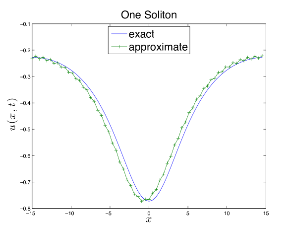
Figure 4.1. Comparison of exact and numerical solutions with initial data (4.1).

We have also computed numerically the error for a range of ${\Delta x}$, where the relative $L^{2}$ error at time $T$ is defined by

$$E1(T)=100\frac{\left\|u-u_{{\Delta x}}\right\|_{2}}{\left\|u\right\|_{2}}$$

where the norms were computed using the trapezoid rule on the points $x_{j}$, and the relative $L^{\infty}$ error is defined by

$$E2(T)=100\frac{\left\|u-u_{{\Delta x}}\right\|_{\infty}}{\left\|u\right\|_{\infty}}.$$

In Table 4.1, we show $L^{2}$ relative errors as well as $L^{\infty}$ relative errors for this example at time $T=480$.

$N$	$E1$	rate	$E2$	rate
33	21.24		23.35
65	5.76	1.9	6.75	1.8
129	1.46	2.0	1.71	2.0
257	0.39	1.9	0.49	1.8
513	9.75e-2	2.0	1.21e-1	2.0
1025	3.34e-2	1.5	4.70e-2	1.4
2049	7.50e-3	2.1	1.07e-2	2.1

Table 4.1. $E1$ and $E2$ for the one-soliton solution at time $T=480$.

The computed solution in Figure 4.1 looks quite well and the errors are also quite low and the convergence rate seems to converge to 2.

4.1. A two-soliton solution

The velocity of a soliton depends on its amplitude; the higher the amplitude, the faster it moves. Thus a fast soliton will overtake a slower soliton moving in the same direction. After the interaction, the solitons will reappear with the same shape, but possibly with a change in phase. As explicit formulas are available, they provide excellent test cases for numerical methods.

Inspired by [19] we use the exact solution

(4.2) $$w(x,t)=-\frac{4c_{1}c_{2}\left(c_{1}\lambda^{2}_{1}+c_{2}\lambda^{2}_{2}+(c_{1}+c_{2})^{3}c_{1}^{-1}c_{2}^{-1}(c_{1}-c_{2})^{-2}\right)}{\left(c_{1}c_{2}\lambda_{1}\lambda_{2}-(c_{1}+c_{2})^{2}(c_{1}-c_{2})^{-2}\right)^{2}+(c_{1}\lambda_{1}+c_{2}\lambda_{2})^{2}},$$

where $\lambda_{j}=\lambda_{j}(x,t)=x-c_{j}t$, $j=1,2$, and $c_{1},c_{2}$ are arbitrary constants. Explicit periodic two-soliton solutions exist, but the exact formula is complicated. See, e.g., [16] for a more detailed discussion. In what follows, we have computed the two-soliton solution (4.2) of the unrestricted Cauchy problem (1.2). Moreover, we have used the initial value $u_{0}(x)=w(x,-10)$ on an interval $(-30,30)$ as initial values. and $c_{1}=2$, $c_{1}=1$. Since we compute on a finite line we have used the periodic continuation, and used the scheme for the periodic case. Since $w(\pm 30,t)$ remains very small in the time interval $[-10,10]$ we believe that the computed solution is very close to $w(t-10,x)$ for $t\leq 20$, and we use $w(10,x)$ as a reference solution.

Computationally, this is a much harder problem than the one-soliton solution due to the fact that in this case the errors stem from both the approximation of the unrestricted initial-value problem by a periodic one, and by the numerical approximation of the latter. In Figure 4.2 we show the exact solution and the approximate solutions at $t=20$ computed using $257$ and $513$ grid points in the interval $[-30,30]$.

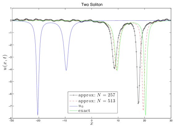
Figure 4.2. The numerical solution $u_{\Delta x}(x,20)$ with initial data $w(x,-10)$.

As the Figure 4.2 exhibits, the scheme performs well in the sense that after the interaction, the two soliton have the same shapes and velocities as before the interaction. In Table 4.2, we show the relative errors $E1$ and $E2$ as well as numerical rate of convergence for the computed solutions. The large errors and the slow convergence rate both indicate that we are not yet in asymptotic regime.

$N$	$E1$	rate	$E2$	rate
65	125.12		113.07
129	124.76	0.0	97.26	0.2
257	108.74	0.2	93.99	0.0
513	71.34	0.6	71.20	0.4
1025	25.28	1.5	29.20	1.3
2049	6.87	1.9	7.98	1.9
4097	2.16	1.7	2.52	1.7

Table 4.2. $E1$ and $E2$ for the two-soliton solution at time $T=20$ with initial data $w(-10,x)$.

To sum up, our conservative scheme performs very well in practice and proven to converge, whereas to the best of our knowledge, there is no constructive proof of convergence, for the other schemes associated to (1.1) or (1.2), except [19] for some partial result (existence of solution has been assumed) in the periodic case (1.2).

References

• [1] M.  J. Ablowitz and A.  S. Fokas. The inverse scattering transform for the Benjamin–Ono equation, a pivot for multidimensional problems. Stud. Appl. Math. 68:1–10 (1983).
• [2] T. B. Benjamin. Internal waves of permanent form in fluid of great depth. J. Fluid. Mech. 29:559–592 (1967).
• [3] J. P. Boyd and Z. Xu. Comparison of three spectral methods for the Benjamin–Ono equation: Fourier pseudospectral, rational Christov functions and Gaussian radial basis functions. Wave Motion 48:702–706 (2011).
• [4] N. Burq and F. Planchon. On well-posedness for the Benjamin–Ono equation. Math. Ann. 340:497–542 (2008).
• [5] Z. Deng, and H. Ma. Optimal error estimates of the Fourier spectral method for a class of nonlocal, nonlinear dispersive wave equations. Appl. Numer. Math. 59:988–1010 (2009).
• [6] R. Dutta, H. Holden, U. Koley, and N. H. Risebro. Operator splitting schemes for the Benjamin–Ono equation. Preprint, 2015.
• [7] H. Holden, U. Koley, and N. H. Risebro. Convergence of a fully discrete finite difference scheme for the Korteweg–de Vries equation. IMA J. Numer. Anal., doi:10.1093/imanum/dru040.
• [8] A.  Ionescu, and C.  E. Kenig. Global well posedness of the Benjamin–Ono equation in low regularity spaces. J. Amer. Math. Soc., 20:753–798 (2007).
• [9] R.  Iorio. On the Cauchy problem for the Benjamin–Ono equation. Comm. Part. Diff. Eq., 11:1031–1081 (1986).
• [10] F. W. King. Hilbert Transforms. Vol. $1$. Cambridge UP, Cambridge (2009).
• [11] L. Molinet. Global well-posedness in $L^{2}$ for the periodic Benjamin–Ono equation. Amer. J. Math. 130:635–683 (2008).
• [12] H. Ono. Algebraic solitary waves in stratified fluids. J. Phy. Soc. Japan 39(4):1082–1091 (1975).
• [13] B. Pelloni and V. A. Dougalis. Numerical solution of some nonlocal, nonlinear dispersive wave equations. J. Nonlinear. Sci. 10:1–22 (2000).
• [14] B. Pelloni and V. A. Dougalis. Error estimate for a fully discrete spectral scheme for a class of nonlinear, nonlocal dispersive wave equations. Appl. Numer. Math. 37:95–107 (2001).
• [15] G. Ponce. On the global well posedness of the Benjamin–Ono equation. Diff. Int. Eq. 4:527–542 1991).
• [16] J. Satsuma, and Y. Ishimori. Periodic wave and rational soliton solutions of the Benjamin–Ono equation. J. Phys. Soc. Japan. 46:681–687 (1979).
• [17] A. Sjöberg. On the Korteweg–de Vries equation: Existence and uniqueness. J. Math. Anal. Appl. 29:569–579 (1970).
• [18] T. Tao. Global well-posedness of the Benjamin–Ono equation in $H^{1}(\mathbb{R})$. J. Hyp. Diff. Equations 1(1):27–49 (2004).
• [19] V. Thomee and A. S. Vasudeva Murthy. A numerical method for the Benjamin–Ono equation. BIT 38(3):597–611 (1998).