Bernoulli-Gaussian Approximate Message-Passing Algorithm for Compressed Sensing with
1D-Finite-Difference Sparsity

Abstract

This paper proposes a fast approximate message-passing (AMP) algorithm for solving compressed sensing (CS) recovery problems with 1D-finite-difference sparsity in term of MMSE estimation. The proposed algorithm, named ssAMP-BGFD, is low-computational with its fast convergence and cheap per-iteration cost, providing phase transition nearly approaching to the state-of-the-art. The proposed algorithm is originated from a sum-product message-passing rule, applying a Bernoulli-Gaussian (BG) prior, seeking an MMSE solution. The algorithm construction includes not only the conventional AMP technique for the measurement fidelity, but also suggests a simplified message-passing method to promote the signal sparsity in finite-difference. Furthermore, we provide an EM-tuning methodology to learn the BG prior parameters, suggesting how to use some practical measurement matrices satisfying the RIP requirement under the ssAMP-BGFD recovery. Extensive empirical results confirms performance of the proposed algorithm, in phase transition, convergence speed, and CPU runtime, compared to the recent algorithms.

I Introduction

I-A Background

We consider compressed sensing (CS) recovery problems for estimating piecewise-constant (PWC) signals $\underline{X}\in\mathbb{R}^{N}$, whose sparsity is in its 1D-finite-difference (FD), from noisy measurements $\underline{Y}\in\mathbb{R}^{M}$ given by

$$\underline{Y}={\mathbf{H}}\underline{X}+\underline{W},$$ (1)

where $\underline{W}\in\mathbb{R}^{M}$ is handled as an AWGN vector, and ${\mathbf{H}}\in{\mathbb{R}^{M\times N}}$ is a measurement matrix. In particular, we deal with incomplete measurements $\underline{Y}$ such that the linear system (1) is underdetermined, meaning that the number of measurements $M$ is significantly smaller than the signal length $N$ $(M\ll N)$.

The 1D-PWC signal model has been mainly used in bioinformatics or computational biology applications such as genomic data analysis [1],[2],[9] and analysis of molecular dynamics for bacteria [3],[4]. For such applications, compressed sensing can be a promising DSP technique with its dimensionality reduction and sparsity-based denoising abilities because the biological signals/data are basically noisy, requiring large memory storage for its huge datasize. We further introduce an excellent work of Little and Jones discussing various types of the PWC signal model and its applications [5].

Since the solution finding of (1) is ill-posed, optimization methods with regularization have been mostly considered. This allows us to pick an unique point ${\widehat{\underline{X}}}$ from the solution space by imposing a suitable regularizer of $\underline{X}$. The most classical regularizer to the present problem is total variation (TV) [6]. In the TV method, the sparsity of $\underline{X}$ can be promoted by applying an 1D-FD operator defined as ${\mathbf{D}}\underline{X}={[{X_{2}}-{X_{1}},{X_{3}}-{X_{2}},...,{X_{N}}-{X_{N-1}}]^{T}}$. Then, the TV regularization is represented as a non-smooth convex optimization [7],[8], given as

$${\widehat{\underline{X}}}=\arg\mathop{\min}\limits_{\underline{X}}\left\|{\underline{Y}-{\mathbf{H}}\underline{X}}\right\|_{2}^{2}+{\lambda}||{\mathbf{D}}\underline{X}|{|_{1}},$$ (2)

where the parameter $\lambda>0$ controls the balance between the FD sparsity and measurement fidelity which is measured by the squared-error term $\left\|{\underline{Y}-{\mathbf{H}}\underline{X}}\right\|_{2}^{2}$. In statistics area, the optimization method (2) is called Fused Lasso [9].

One popular approach for solving (2) is to use the first-order algorithms which provide global convergence in the general class of convex optimizations, whose convergence rate can be accelerated by applying the Nesterov’s method [53]. As practical first-order solvers, Chambolle-Pock (TV-CP) [10], Fast Iterative Soft-Thresholding Algorithm (FISTA) [11], and Efficient Fused Lasso (EFLA) [12] have been highlighted recently.

I-B Contribution

In the present work, we revisit the CS recovery problem with the Bayesian philosophy, recasting the problem to

$$\begin{gathered}\underline{\widehat{X}}=\arg\min_{\underline{x}}\int{\int{{{(\underline{x}-\widehat{\underline{x}})}^{2}}{f_{\underline{X},\underline{Y}}}(\underline{x},\underline{y})d\underline{x}d\underline{y}}}\hfill\\ \,\,\,\,\,\,\,\,=\frac{1}{Z}\int{\underline{x}\,\underbrace{{f_{\underline{X}}}(\mathbf{D}\underline{x})}_{\text{Prior}}\underbrace{\mathcal{N}(\mathbf{H}\underline{x};\underline{y},\Delta)}_{\text{Likelihood}}d\underline{x}}\hfill\\ \end{gathered}$$ (6)

by applying minimum-mean-square-error (MMSE) estimation method [62], where $Z>0$ is a normalization constant independent of $\underline{x}$. The main advantage of the MMSE method over the TV method (2) is the MMSE-optimality. It guarantees better reconstruction quality in terms of MSE if the signal statistics has a good match with the given prior ${f_{\underline{X}}}(\cdot)$ [16],[17],[62]. On the other hand, one critical disadvantage is analytical intractability of the integral calculation of (6).

The main focus of this paper is on low-computational solving of the CS recovery with the 1D-FD sparsity, and for this purpose we approach the MMSE estimation (6) using Bayesian approximate message-passing (AMP) which is an approximate loopy belief propagation (BP) based on the central-limit-theorem (CLT) [13]-[19]. This is motivated by the fact that the “sum-product” mode of the Bayesian AMP provides accurate and low-computational approximation to the posterior information for (6), which have been demonstrated in the CS recovery with direct sparsity [16]-[19]. The AMP approach also has shown their usefulness by providing own mean-square-error (MSE) prediction method, called state evolution [13],[15],[21].

To the MMSE method (6), we propose a Bayesian AMP algorithm using a Bernoulli-Gaussian (BG) prior. We adopt the BG prior as a key to resolve the analytical intractability of the MMSE method. The proposed AMP is referred to as Spike-and-Slab Approximate Message-Passing using Bernoulli-Gaussian finite-difference prior (ssAMP-BGFD), which was partially introduced in our short paper [24]. We claim that ssAMP-BGFD has advantages in the present CS reconstruction problem, as following:

• ssAMP-BGFD shows phase transition (PT) closely approaching to the state-of-the-art performance.

• ssAMP-BGFD provides low-computationality which is originated from its cheap per-iteration cost with $\mathcal{O}(MN)$ and its fast convergence characteristic.

• ssAMP-BGFD is compatible with several non-i.i.d.-random matrices $\mathbf{H}$.

• ssAMP-BGFD optionally provides Expectation-Maximization (EM) tuning for prior parameters. Therefore, ssAMP-BGFD can be parameter-free.

Each statement claimed above will be discussed and validated in the main body of this paper.

TVAMP, proposed by Donoho et al. in [22], can be considered as another AMP option for the present problem, which is an extension of the standard AMP [13] applying an anisotropic TV denoising to estimate $\underline{X}$. Therefore, TVAMP has a simple algorithmic structure, providing highly fast solution to the problem. However, our empirical result reveals that its PT characteristic is apart from the state-of-the-art.

While working on ssAMP-BGFD, we became aware of an relevant AMP work by Schniter et al., named GrAMPA [20], which was carried out independently and concurrently with our work. The GrAMPA algorithm is based on a novel configuration of the generalized AMP (GAMP) package [16] for the analysis CS setup [33], providing the both Bayesian options: MMSE and MAP estimation. Therefore, it is not confined to this CS problem with 1D-FD sparsity, but being applicable to the problem with generalized sparsity. In addition, it has been empirically confirmed that GrAMPA shows the state-of-the-art PT performance in the CS recovery with 1D-FD sparsity [24].

We argue that ssAMP-BGFD is practically advantageous over TVAMP and GrAMPA for the present problem. ssAMP-BGFD provides its solution $\widehat{\underline{X}}$ as simple and fast as TVAMP does, while showing PT characteristic nearly approaching to the state-of-the-art by GrAMPA. In addition, TVAMP and GrAMPA require parameter configuration before running it, whereas ssAMP-BGFD does not with an auto-parameter tuning by an Expectation Maximization (EM) technique. Furthermore, we empirically demonstrate that column-sign-randomization [48],[49] enables ssAMP-BGFD to work well with practical non-i.i.d.-random matrices satisfying the RIP requirement: sub-sampled Discrete Cosine and Walsh-Hadamard Transforms, quasi-Toeplitz, and deterministic bipolar (proposed in [61]) matrices. We also check the compatibility of ssAMP-BGFD with random sparse matrices.

I-C Organization and Notation

The remainder of the paper is organized as follows. Section II is devoted for a brief introduction to the AMP fundamental and the two existing AMP algorithms for the CS recovery with 1D-FD sparsity: TVAMP [22] and GrAMPA [20]. Section III describes the construction details of the proposed algorithm, ssAMP-BGFD. In Section IV, we provides extensive empirical results to validate several aspects of the ssAMP-BGFD algorithm, compared to the two AMP-based solvers, TVAMP and GrAMPA, as well as the two first-order solvers for the TV method (2), Efficient Fused Lasso [12] and Chambolle-Pock [10]. In Section V, we provide a practical example of the ssAMP-BGFD recovery to a genomic data set. Finally, we conclude this paper in Section VI.

Throughout the paper, we use the following notation. We use underlined letter like $\underline{h}$ to denote vectors, boldface capital letters like $\mathbf{H}$ to denote matrices, and calligraphic capital letters like $\mathcal{F}$ to indicate set symbols. The vectors $\underline{1}\equiv[1,...,1]^{T}$ and $\underline{0}\equiv[0,...,0]^{T}$ denote an one vector and a zero vector respectively. In addition, $f_{X_{i}}(x_{i})$ is a probability density function (PDF) of a random variable $X_{i}\sim f_{X_{i}}(x_{i})$ and its realization is denoted by small letters like $x_{i}$. We use $\mathbb{E}_{f_{X_{i}}}[\cdot]$, $\mathbf{Var}_{f_{X_{i}}}[\cdot]$, and $\mathbb{H}({f_{X_{i}}})$ to denote the expectation, the variance, and the information entropy with respect to the PDF ${f_{X_{i}}(x)}$, respectively. For PDF notation, we use $\mathcal{N}(x_{i};\mu,{\sigma^{2}})\equiv\frac{1}{{\sqrt{2\pi{\sigma^{2}}}}}\exp\left({-\frac{{{{(x_{i}-\mu)}^{2}}}}{{2{\sigma^{2}}}}}\right)$ to denote a Gaussian PDF with mean $\mu$ and variance $\sigma^{2}$, and use $\mathcal{U}({x_{i}};\frac{1}{N})$ to denote a discrete uniform PDF with $N$ points. Finally, we use notation ${\left\langle\underline{v}\right\rangle}\equiv\frac{1}{N}\sum\nolimits_{i=1}^{N}{v_{i}}$ for the sample mean of a certain vector $\underline{v}\in\mathbb{R}^{N}$ and $\eta^{\prime}(\cdot)\equiv\frac{\partial}{{\partial\rho}}\eta(\cdot)$ for the first derivative of the function $\eta(\cdot)$.

II AMP Algorithms:
Fundamental and Related Works

The AMP algorithm was originally proposed by Donoho et al. to solve the CS recovery problem with direct sparsity [13],[14]. The AMP solution $\widehat{\underline{X}}^{(t)}=\underline{\mu}^{(t)}$ is found by a simple iteration according to: for the iteration index $t=0,1,2,...$,

$${\underline{\mu}^{(t+1)}}=\eta({{\mathbf{H}}^{T}}{\underline{r}^{(t)}}+{\underline{\mu}^{(t)}})$$ (7)

$${\underline{r}^{(t)}}=\underline{y}-{\mathbf{H}}{\underline{\mu}^{(t)}}+{\underline{r}^{(t-1)}}\begin{array}[]{l}\frac{N}{M}\end{array}\left\langle{\eta^{\prime}({{\mathbf{H}}^{T}}{{\underline{r}}^{(t-1)}}+{{\underline{\mu}}^{(t-1)}})}\right\rangle$$ (9)

where ${\underline{r}^{(t)}}\in\mathbb{R}^{M}$ denotes a residual vector measuring fidelity from $\underline{y}$ at hand, and $\eta(\cdot):\mathbb{R}^{N}\to\mathbb{R}^{N}$ indicates a denoising function, simply called denoiser, to realize the sparse signal estimate $\underline{\mu}^{(t)}\in\mathbb{R}^{N}$. It is known that the AMP iteration (7) achieves the PT performance equivalent to that of the Lasso method in the large limit of $N,M\to\infty$ and $t\to\infty$ [13],[15],[21]. In addition, the AMP algorithm is basically low-computational with $\mathcal{O}(MN)$ per-iteration cost. Motivated by such excellent properties, recently, there have been several AMP extensions with the various types of sparsity:

• For FD sparsity: TVAMP [22], AMP with non-local mean denoiser [23], ssAMP-BGFD [24],

• For group sparsity: Block-AMP [22],[30]

• For complex valued sparsity: Complex-AMP [29]

• For wavelet sparsity: AMP with amplitude-scale-invariant Bayes’estimator [31], Turbo-AMP with hidden Markov tree [32]

• For generalized sparsity: GrAMPA [20]

The practical use of the AMP algorithms is not straightforward. This is mainly caused by the fact that AMP basically postulates the matrix entries $h_{ji}\in\mathbf{H}$ following the i.i.d. statistics of $\mathbb{E}[h_{ji}]=0$ and $\text{Var}[h_{ji}]=\frac{1}{M}$. This postulation is essential to guarantee the AMP convergence and validate the state evolution method providing the own MSE prediction [15],[21],[58]. However, the postulation largely limits practical applicability of the AMP algorithms for the three main reasons as given below:

• Statistical inconsistency in small systems: The law of large number does not hold with small $(M,N)$ such that the sample mean and variance of $h_{ji}$ may not be consistent with $\mathbb{E}[h_{ji}]=0$ and $\text{Var}[h_{ji}]=\frac{1}{M}$.

• No fast implementation of matrix-vector multiplication: The matrix-vector multiplication takes $\mathcal{O}(MN)$ complexity, which is a computational bottleneck in AMP. This can be relaxed by fast implementation methods, such as Fast Fourier Transform (FFT), when $\mathbf{H}$ is some unitary or Toeplitz matrices. In such cases, the complexity is reduced to $\mathcal{O}(N\log N)$ [50]. However, there are no such methods for the i.i.d.-random matrices.

• Large memory for storage: In general, the pure i.i.d.-random matrices $\mathbf{H}$ densely include $\mathcal{O}(MN)$ independent random variables. Hence, its matrix storage requires significant space with large $(M,N)$.

To overcome these limitations, sub-sampled unitary matrices, such as Discrete Cosine Transform (DCT) matrix, have been tested with AMP, reporting successful results for implementation and performance both [17],[52]. As another direction, some researchers have attempted to operate the AMP algorithms with generic matrices $\mathbf{H}$ by using “damping” [25],[26], “mean-removing” [25], “serial updating” [27], and “free-energy minimization” [28]. These approaches generally improve stability of the AMP convergence at the expense of its recovery speed.

In [16], Rangan extended the standard AMP (7) to signals $\underline{X}$, whose elements are drawn from generalized i.i.d. PDFs, by applying Bayesian philosophy, solidifying the foundation for Bayesian AMP works: [17]-[20],[24],[25],[28],[32]. In the work of [16], Rangan classifies the Bayesian AMP into two modes according to its signal estimation criterion.

• Max-sum mode: The mode is originated from the max-sum loopy BP for the MAP estimation of $\underline{X}$. Therefore, the denoiser for this mode estimates the signal by solving a sub-optimization defined as

  $$\begin{array}[]{l}\eta(\underline{\rho})\equiv\arg\mathop{\min}\limits_{\underline{X}}\frac{1}{2}||\underline{\rho}-\underline{X}||_{2}^{2}+g(\mathcal{T}\underline{X}).\end{array}$$ (11)

• Sum-product mode: The mode is based on the sum-product loopy BP for the MMSE estimation of $\underline{X}$. Hence, the denoiser for this mode generates the signal by solving a sub-optimization given as

  $$\eta(\underline{\rho})\equiv\frac{1}{Z}\int{\underline{x}\exp\left(-\frac{1}{2}||\underline{\rho}-\underline{x}||_{2}^{2}-g(\mathcal{T}\underline{x})\right)d\underline{x}}.$$ (12)

In (11) and (12), $\underline{\rho}\in\mathbb{R}^{N}$ is the denoiser input, $\mathcal{T}$ is an analysis operator, and $Z>0$ is a normalization constant. In the Bayesian AMP, the regularizer is a functional of the signal prior $f_{\underline{X}}(\mathcal{T}\underline{x})$, i.e., $g:V\to\mathbb{R}$ where $V\equiv\{{f_{\underline{X}}}:{\mathbb{R}^{N}}\to[0,1]\}$, which controls the denoising behavior for enhancing the signal sparsity in the domain of $\mathcal{T}$.

In the remaining of this section, we briefly introduce the two existing AMP algorithms applicable to the CS recovery with 1D-FD sparsity: TVAMP [22] and GrAMPA [20], by focusing on their denoisers $\eta(\cdot)$. These two algorithms will be included for the simulation-based comparison to the proposed AMP algorithm, ssAMP-BGFD, in Section IV.

II-A TVAMP Algorithm

Donoho et al. introduced TVAMP for the present problem. [22]. TVAMP uses the standard AMP iteration, given in (7), with an anisotropic TV denoiser. TVAMP is classified to the “max-sum” mode such that its denoiser can be represented in the form of the MAP estimation (11), i.e.,

$$\begin{array}[]{l}\eta(\underline{\rho})\equiv\arg\mathop{\min}\limits_{\underline{X}}\frac{1}{2}\left\|{\underline{\rho}-\underline{X}}\right\|_{2}^{2}+\lambda||\mathbf{D}\underline{X}||_{1},\end{array}$$ (14)

where the sparsity is enhanced with the $l_{1}$-regularizer such that $g(\mathcal{T}\underline{X})\equiv\lambda||\mathbf{D}\underline{X}||_{1}$, meaning from a Bayesian viewpoint that Laplacian prior is imposed. The implementation denoiser of (14) requires an numerical TV minimizer, such as FLSA [41], TVDIP [34], FISTA-TV [11], and Condat’s direct method [56], since the optimization (14) is neither scalar-separable nor smooth such that no closed-form solutions exist. Therefore, complexity of TVAMP highly depends upon that of the numerical minimizer.

The minimizer for (14) requires batch vector computation, leading to the non-separability of the TV denoiser. Namely, the denoising operations is not coordinatewise as illustrated in Fig.2. This non-separability prevents TVAMP from characterizing its MSE in terms of a scalar equivalent model, which deprives TVAMP of mathematical completeness for its state evolution formalism [15],[21],[22]. The non-separability does not mean that TVAMP is not scalable for large-scale problems. TVAMP can have very good scalability for large $N,M$ according to choice of the numerical TV minimizer (see Section IV-C for its validation).

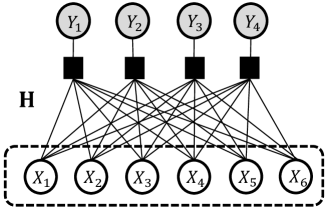
Figure 1: Factor graphical modeling of the linear system (1) having a PWC solution $\underline{X}$, used by the two AMP algorithms: ssAMP-BGFD (proposed) and the GrAMPA [20], where the denoiser $\eta(\cdot)$, indicated by dotted-line boxes in this figure, scalar-separablely works.

Figure 2: Factor graphical modeling of the linear system (1) having a PWC solution $\underline{X}$, used by the TVAMP algorithm [22], where the non-scalar-separable denoiser $\eta(\cdot)$, indicated by a dotted-line box in this figure, is a batch vector function.

II-B GrAMPA Algorithm

Recently, Schniter et al. introduced the GrAMPA algorithm for the analysis CS setup [20]. GrAMPA is useful for general CS recovery problems with arbitrary analysis operators $\mathcal{T}$, arbitrary independent signal priors $g(\mathcal{T}\underline{x})\propto\sum\nolimits_{d}{g_{d}([\mathcal{T}\underline{x}]_{d})}$, and arbitrary independent likelihood $\sum\nolimits_{j}{\log f_{Y_{j}}(y_{j}|{{[\mathbf{H}\underline{x}]}_{j}})}$. Namely, GrAMPA has very good universality to signal and noise models. Hence, this GrAMPA framework can be simply configured for the present problem by setting $\mathcal{T}=\mathbf{D}$ and by assuming the AWGN model. The corresponding factor graph model is shown in Fig.2.

GrAMPA supports the both modes of the Bayesian AMP. In the present work, we are interested in the “sum-product” mode for the method (6), therefore focusing on the MMSE-based denoiser in the form of (12), expressed as

$$\eta(\underline{\rho})\equiv\frac{1}{Z}\int{\underline{x}\exp\left(-\frac{1}{2}||\underline{\rho}-\underline{x}||_{2}^{2}-\sum\limits_{d=1}^{N-1}g_{d}([\mathbf{D}\underline{x}]_{d};\widehat{U}_{d})\right)d\underline{x}},$$ (15)

where the authors suggests to use the regularizer $g_{d}([\mathbf{D}\underline{x}]_{d};\widehat{U}_{d})$ with an MMSE estimate of a FD scalar:

$$\widehat{U}_{d}\equiv{\mathbb{E}}\left[U_{d}|[\mathbf{D}\widehat{\underline{x}}]_{d},v_{d}\right]=\frac{[\mathbf{D}\widehat{\underline{x}}]_{d}}{1+\omega\mathcal{N}(0;[\mathbf{D}\widehat{\underline{x}}]_{d},{\nu_{d}})}.$$ (16)

In (15) and (16), we define the random variable $U_{d}\in\mathbb{R}$ as a clean FD scalar, assuming that the current signal estimate $\widehat{\underline{X}}$ is noisy such that $[\mathbf{D}\widehat{\underline{X}}]_{d}=U_{d}+W^{\prime}$ where $W^{\prime}\sim\mathcal{N}(0,\nu_{d})$. The authors named this denoiser with (15) and (16) as the SNIPE denoiser. The SNIPE denoiser can support any Bernoulli-* prior, where “*” is any continuous PDF, by controlling the parameter $\omega>0$.

The naive per-iteration cost of GrAMPA is $\mathcal{O}(N^{2}+MN-N)\approx\mathcal{O}(N^{2})$ because GrAMPA operates by the GAMP package with an augmented linear transform $\mathbf{H}^{\prime}=\left[{\frac{{\mathbf{H}}}{{\mathbf{D}}}}\right]\in\mathbb{R}^{M+N-1\times N}$. However, its complexity is simply reduced to $\mathcal{O}(MN)$ using a fast sparse multiplication method to $\mathbf{H}^{\prime}$ [43].

III Proposed Algorithm

In this section, we introduce the proposed algorithm, ssAMP-BGFD, for solving (6) We describe the details of the algorithm construction: from its factor graphical modeling to the AMP approximation. Then, we finalize this section with discussion about the prior parameter learning by an EM-tuning method. The overall iteration of ssAMP-BGFD is summarized in Algorithm 2.

III-A Factor Graphical Model and Prior Model

The statistical dependency of linear systems have been effectively modeled using factor graphs [39]. Let $\mathcal{V}\equiv\{1,...,N\}$ be a variable set whose element $i\in\mathcal{V}$ corresponds to a signal scalar $X_{i}$, and $\mathcal{F}_{m}\equiv\{1,...,M\}$ be a factor set whose element $j\in\mathcal{F}_{m}$ corresponds to a measurement scalar $Y_{j}$. To the problem, we include another factor set, defined as $\mathcal{F}_{s}\equiv\{1,...,N-1\}$, to describe statistical connections of a finite-difference (FD) scalar $\forall d\in\mathcal{F}_{s}:U_{d}=[\mathbf{D}\underline{X}]_{d}$. In order to clarify two different factors, we name the set $\mathcal{F}_{m}$ as m-factor set, and the set $\mathcal{F}_{s}$ as s-factor set. Then, a factor graph, denoted by $\mathcal{G}(\mathcal{V},{\mathcal{F}_{m}},{\mathcal{F}_{s}})$, fully models the linear system (1) with a 1D-PWC solution $\underline{X}$, as shown in Fig.2. This graph modeling approach enables us to devise a message-passing rule for statistically connected signals, which is related to the approach of Hybrid-GAMP [40] and also used in GrAMPA [20]. In addition, for convenience, we indicate the neighboring relation between the two sets, $\mathcal{V}$ and $\mathcal{F}_{s}$, by defining $\forall i\in\mathcal{V}:ne(i)\equiv\{d_{1},d_{2}\in\mathcal{F}_{s}|d_{1}=i-1,d_{2}=i\}$ and $\forall d\in\mathcal{F}_{s}:ne(d)\equiv\{i_{1},i_{2}\in\mathcal{V}|i_{1}=d,i_{2}=d+1\}$.

Based on the graph model designed above, we represent the joint PDF of the linear system (1) as

$${f_{\underline{X},\underline{Y}}}(\mathbf{D}\underline{x},\underline{y})=\frac{1}{Z}\underbrace{\prod\limits_{d\in\mathcal{F}_{s}}{{f_{U_{d}}}(u_{d})}}_{\text{Prior}}\underbrace{\prod\limits_{j\in\mathcal{F}_{m}}{{f_{{Y_{j}}|\mathbf{H}\underline{X}}}({y_{j}}|\mathbf{H}\underline{x})}}_{\text{Likelihood}}$$ (17)

where $Z\in\mathbb{R}$ is a normalization constant to validate $\int{{f_{\underline{X},\underline{Y}}}(\mathbf{D}\underline{x},\underline{y})d\underline{x}d\underline{y}=1}$. To each m-factor $j\in\mathcal{F}_{m}$, we consider an independent Gaussian likelihood function, i.e.,

$${{f_{{Y_{j}}|\underline{X}}}({y_{j}}|\mathbf{H}\underline{x})}=\mathcal{N}(y_{j};\left(\mathbf{H}\underline{x}\right)_{j},\Delta),$$ (18)

for our AWGN noise model where $\Delta$ is the noise variance.

To each s-factor $d\in\mathcal{F}_{s}$, we impose an independent Bernoulli-Gaussian (BG) prior for a FD scalar, $\forall i_{1},i_{2}\in ne(d):u_{d}=[\mathbf{D}\underline{x}]_{d}=x_{i_{1}}-x_{i_{2}}$, by assuming its sparsity. The BG prior takes a form of the spike-and-slab PDFs [59], which is given as

$${f_{U_{d}}}(u_{d}=x_{i_{1}}-x_{i_{2}})=(1-q)\delta(u_{d})+q\mathcal{N}(u_{d};0,\sigma_{0}^{2})$$ (19)

where $\delta(u_{d})$ denote a Dirac function peaked at $u_{d}=0$, $q\in[0,1]$ is a probability weight, and $\sigma_{0}^{2}\in(0,\infty)$ is the variance of the Gaussian PDF. Following that, the number of nonzeros in FD of $\underline{X}$ is explicitly Binomial random with $K\sim\mathcal{B}(N-1,q)$. Such a BG prior (19) has been widely used in the CS literature with respect to Bayesian algorithms [17]-[20],[35]-[37] because

1. the PDF has a sparsifying ability,

2. the integration of the PDF is tractable with its Gaussianity, and

3. the PDF is simply parameterized.

Although one recent paper [57] pointed out that the BG prior PDF is not appropriate for dealing with discretized continuous-time signals due to its fast decayed tail, we argue that the BG prior is still a powerful choice for parametric algorithms, which keep track a set of statistical parameters such as mean and variance, by its analytical tractability [17],[19].

Algorithm 1 Sum-Product Rule

for $t=1$ to $t^{*}$ do

     Variable to s-factor (V2sF) update

    $\forall(d,i)\in\mathcal{F}_{s}\times\mathcal{V}\text{ and }d,d^{\prime}\in ne(i):$

    $\widehat{v}_{i\to d}^{(t+1)}({x_{i}})=\frac{1}{\widetilde{Z}_{i\to d}}s_{d^{\prime}\to i}^{(t)}({x_{i}})\prod\limits_{j\in\mathcal{F}_{m}}{m_{j\to i}^{(t)}({x_{i}})}\,\,(d\neq d^{\prime})$

     s-factor to variable (sF2V) update

    $\forall(d,i)\in\mathcal{F}_{s}\times\mathcal{V}\text{ and }i,i^{\prime}\in ne(d):$

    $s_{d\to i}^{(t)}({x_{i}})=\mathbb{E}_{\widehat{v}_{i^{\prime}\to d}^{(t)}(x_{i}^{\prime})}\left[{f_{U_{d}}}(u_{d}={x_{i}}-{x_{i^{\prime}}})|x_{i^{\prime}}\right]\,\,(i^{\prime}\neq i)$

     Variable to m-factor (V2mF) update

    $\forall(j,i)\in\mathcal{F}_{m}\times\mathcal{V}:$

    $v_{i\to j}^{(t+1)}({x_{i}})=\frac{1}{Z_{i\to j}}\prod\limits_{d\in ne(i)}{s_{d\to i}^{(t)}({x_{i}})}\prod\limits_{j^{\prime}\neq j}{m_{j^{\prime}\to i}^{(t)}({x_{i}})}$

     m-factor to variable (mF2V) update

    $\forall(j,i)\in\mathcal{F}_{m}\times\mathcal{V}:$

    $m_{j\to i}^{(t)}({x_{i}})=\mathbb{E}_{\{v_{i^{\prime}\to j}^{(t)}(x_{i}^{\prime})\}}\left[{f_{{Y_{j}}|\mathbf{H}\underline{X}}}({y_{j}}|\mathbf{H}\underline{x})|{\{x_{i^{\prime}}\}}\right]\,\,(i^{\prime}\neq i)$

end for

III-B Sum-Product Belief Propagation for MMSE Estimation

We now make use of the factor graphical model of Fig.2 to derive an efficient recovery algorithms for the present problem. We approach the problem through the MMSE method, which lead us to the “sum-product” rule of loopy BP [16],[44]. There exists a vast literature justifying the use of the sum-product BP algorithm, applying them on concrete problems such as channel coding [45], computer vision [47], as well as compressed sensing (CS) [37],[38].

We construct a sum-product rule based on the joint PDF of (17), which consists of four types of the local message updates as graphically illustrated in Fig.3 and listed in Algorithm 1, where the expectation of the sF2V and mF2V updates are over the previous V2sF and V2mF messages, respectively; the constants $Z_{i\to j},\widetilde{Z}_{i\to d}>0$ are for normalization. This sum-product task is divided into two parts:

1. Pursuing the 1D-FD sparsity with the independent BG prior (19),

2. Seeking the measurement fidelity with the independent Gaussian likelihood function (18) for the AWGN model.

The first part is with respect to the s-factors $\mathcal{F}_{s}$ (the V2sF and sF2V updates), and the second part is with the m-factors $\mathcal{F}_{m}$ (the V2mF and mF2V updates). Then, at the fixed-point ($t=t^{*}$), the marginal posterior of $X_{i}$ is approximated by

$$f_{X_{i}|\underline{Y}}(x_{i}|\underline{y})\propto\prod\limits_{d\in ne(i)}{s_{d\to i}^{(t=t^{*})}({x_{i}})}\prod\limits_{j\in\mathcal{F}_{m}}{m_{j\to i}^{(t=t^{*})}({x_{i}})}.$$ (20)

Using (20), we provide an MMSE approximation of $\widehat{X_{i}}$, whose function is defined as the denoiser of the ssAMP-BGFD algorithm, i.e.,

$$\mu_{i}={\eta}(\cdot) \equiv\mathbb{E}_{f_{X_{i}|\underline{Y}}}\left[{X_{i}}|{\mathbf{H}},\underline{Y}=\underline{y}\right],$$ (21)

and the corresponding variance function is given as

$$\sigma_{i}^{2}={\gamma}(\cdot) \equiv\mathbf{Var}_{f_{X_{i}|\underline{Y}}}\left[{X_{i}}|{\mathbf{H}},\underline{Y}=\underline{y}\right].$$ (22)

However, as claimed in literature [13]-[19], Algorithm 1 is infeasible in practice because i) the messages are density function over the real line, and ii) $2MN+4(N-1)$ message exchanges are required per iteration.

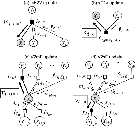
Figure 3: Factor graphical representation of the sum-product rule: (a) m-factor to variable (mF2V) update, (b) s-factor to variable (sF2V) update, (c) variable to m-factor (V2mF) update, (d) variable to s-factor (V2sF) update.

III-C AMP Approximation

We approach the computational infeasibility of Algorithm 1 via the AMP approximation, which have been discussed and analyzed in the literature [13]-[19],[21]. The AMP approximation produces a remarkably simpler algorithm, whose messages are real numbers instead of density functions, which handles $\mathcal{O}(M+N)$ messages rather than $\mathcal{O}(MN)$ messages per iteration. In the conventional literature [13]-[19], this approximation consists of two steps:

• Parameterization step: Based on the central limit theorem (CLT), the sum-product rule is approximated to a parametric message-passing rule exchanging a pair of real numbers,

• First-order approximation step: This step cancels interference caused by the loopy graph connection, leading to reduction of the number of the messages handled in the mF2V and V2mF updates.

In addition to these steps, the present work includes the third step, called Right/Left Toward Message-Passing (R2P/L2P) step, to deal with the sF2V and V2sF updates. This R2P/L2P update is devoted to promote the signal sparsity over the statistical chain connection with $\mathcal{V}$ and $\mathcal{F}_{s}$.

Throughout this AMP approximation, we assume that the matrix $\mathbf{H}$ is a dense i.i.d.-random matrix, i.e., its entries $h_{ji}\in\mathbf{H}$ are randomly distributed with zero mean and variance $\frac{1}{M}$; hence, ${\mathbb{E}}||\underline{h}_{i}||_{2}^{2}=1$. In addition, we clarify beforehand that this AMP approximation is heuristic. Namely, we do not claim any mathematical equivalence between the sum-product rule of Algorithm 1 and the ssAMP-BGFD rule produced by this approximation.

III-C1 STEP I - Parameterization Step

We begin this step with definitions of the mean and variance of $X_{i}$ over the message densities:

$$\mu_{i\to j} = \mathbb{E}_{v_{i\to j}}[X_{i}|{\mathbf{H}},\underline{Y}=\underline{y}],$$ (23a)

$$\sigma_{i\to j}^{2} = \mathbf{Var}_{v_{i\to j}}[X_{i}|{\mathbf{H}},\underline{Y}=\underline{y}],$$ (23b)

$$\mu_{i\to d} = \mathbb{E}_{\widehat{v}_{i\to d}}[X_{i}|{\mathbf{H}},\underline{Y}=\underline{y}],$$ (23c)

$$\sigma_{i\to d}^{2} = \mathbf{Var}_{\widehat{v}_{i\to d}}[X_{i}|{\mathbf{H}},\underline{Y}=\underline{y}].$$ (23d)

For large $N$, we can approximate exponent of the mF2V message by a quadratic function based on CLT; then, the mF2V message becomes a scaled Gaussian PDF [16],[19]. The sF2V message is represented as a Bernoulli-Gaussian PDF by calculating the integration with the BG prior (19). Using these two facts, we specify the message representation from Algorithm 1:

• V2sF messages:

  $$\begin{array}[]{l}{\widehat{v}_{i\to d}}({x_{i}})=\frac{1}{\widetilde{Z}_{i\to d}}{s_{d^{\prime}\to i}}({x_{i}})\mathcal{N}({x_{i}};{\rho_{i}},\theta_{i}),\end{array}$$ (25)

• sF2V messages:

  $$\begin{array}[]{l}{s_{d\to i}}({x_{i}})=(1-q)\mathcal{N}({x_{i}};{\mu_{i^{\prime}\to d}},{\sigma_{i^{\prime}\to d}^{2}})\\ \,\,\,\,\,\,\,\,\,\,\,\,\,\,\,\,\,\,\,\,\,\,\,\,\,\,\,\,\,\,\,\,\,\,\,\,\,\,\,\,+q\mathcal{N}({x_{i}};{\mu_{i^{\prime}\to d}},\sigma_{0}^{2}+\sigma_{i^{\prime}\to d}^{2}),\end{array}$$ (28)

• V2mF messages:

  $$\begin{array}[]{l}{v_{i\to j}}({x_{i}})=\frac{1}{Z_{i\to j}}\prod\limits_{d\in ne(i)}{s_{d\to i}({x_{i}})}{\mathcal{N}({x_{i}};{\rho_{i\to j}},\theta_{i\to j})},\end{array}$$ (30)

• mF2V messages:

  $$\begin{array}[]{l}{m_{j\to i}}({x_{i}})\propto\mathcal{N}\left(h_{ji}{x_{i}};r_{j\to i},\theta_{j\to i}\right),\end{array}$$ (32)

where we need several parameter definitions:

$${\rho_{i\to j}} \equiv \sum\nolimits_{j^{\prime}\neq j}{h_{j^{\prime}i}}{r_{j^{\prime}\to i}},$$ (33a)

$${\rho_{i}} \equiv \sum\nolimits_{j\in\mathcal{F}_{m}}{h_{ji}}{r_{j\to i}},$$ (33b)

$${r_{j\to i}} \equiv {y_{j}}-\sum\nolimits_{i^{\prime}\neq i}{h_{ji^{\prime}}\mu_{i^{\prime}\to j}},$$ (33c)

$${\theta_{j\to i}} \equiv \Delta+\sum\nolimits_{i^{\prime}\neq i}h_{ji^{\prime}}^{2}\sigma_{i^{\prime}\to j}^{2},$$ (33d)

and in the large limit $(M\to\infty)$, the variance parameter ${\theta_{i\to j}}$ can drop its directional nature, i.e.,

$${\theta_{i\to j}}\equiv\sum\limits_{j^{\prime}\neq j}{h_{j^{\prime}i}^{2}{\theta_{j^{\prime}\to i}}}\mathop{=}\limits^{M\to\infty}\frac{1}{M}\sum\limits_{j\in\mathcal{F}_{m}}{{\theta_{j\to i}}}={\theta_{i}}.$$ (34)

Equations (23),(33),(34) establish a message update rule which only exchanges the parameters of the message densities (25)-(32): namely, $(\rho_{i},\theta_{i},\{\mu_{i\to d},\sigma_{i\to d}^{2}\}_{d\in ne(i)})$ for the sF2V and V2sF updates, $(\rho_{i\to j},\theta_{i\to j},\mu_{i\to j},\sigma^{2}_{i\to j})$ for the V2mF update, and $(r_{j\to i},\theta_{j\to i})$ for the mF2V update.

To formulate the calculations of (23) with the parameters we have defined in (33),(34), we further define

$$\eta(\cdot)\equiv\mathbb{E}_{v_{i\to j}}[X_{i}|\rho_{i\to j},\theta_{i},\{\mu_{i\to d},\sigma_{i\to d}^{2}\}_{d\in ne(i)}],$$ (35a)

$$\gamma(\cdot)\equiv\mathbf{Var}_{v_{i\to j}}[X_{i}|\rho_{i\to j},\theta_{i},\{\mu_{i\to d},\sigma_{i\to d}^{2}\}_{d\in ne(i)}],$$ (35b)

$$\phi(\cdot)\equiv\mathbb{E}_{\widehat{v}_{i\to d}}[X_{i}|\rho_{i},\theta_{i},\mu_{i\to d^{\prime}},\sigma_{i\to d^{\prime}}^{2}],$$ (35c)

$$\zeta(\cdot)\equiv\mathbf{Var}_{\widehat{v}_{i\to d}}[X_{i}|\rho_{i},\theta_{i},\mu_{i\to d^{\prime}},\sigma_{i\to d^{\prime}}^{2}].$$ (35d)

The V2mF calculations of (23a),(23b) share the functions, $\eta(\cdot)$ and $\gamma(\cdot)$, with the MMSE approximation of (21),(22), respectively. This is based on the fact that the marginal posterior and the V2mF message are equivalent PDFs except the difference of $\rho_{i}$ and $\rho_{i\to j}$. We can represent the function $\eta(\cdot)$ in the form of an MMSE-based denoiser (12), i.e.,

$$\eta({\rho_{i}};{\theta_{i}},\{\mu_{i^{\prime}\to d},\sigma_{i^{\prime}\to d}^{2}\}_{d\in ne(i)})$$ (36)

$$\equiv\frac{1}{Z}\int{{x_{i}}\exp\left({-\frac{{{({x_{i}}-{\rho_{i}})}^{2}}}{{2{\theta_{i}}}}-{g_{i}}({x_{i}};\{\mu_{i^{\prime}\to d},\sigma_{i^{\prime}\to d}^{2}\})}\right)d{x_{i}}}$$

where the FD sparsity regularizer ${g_{i}}({x_{i}};\cdot)$ is defined as

$${g_{i}}({x_{i}};\{\mu_{i^{\prime}\to d},\sigma_{i^{\prime}\to d}^{2}\})\equiv-\sum\limits_{(d,i^{\prime})}{\log\,{s_{d\to i}}({x_{i}};\mu_{i^{\prime}\to d},\sigma_{i^{\prime}\to d}^{2})}.$$

for $(d,i^{\prime})\in\{({d_{1}},i-1),({d_{2}},i+1)|d_{1},d_{2}\in ne(i)\}$. In addition, we emphasize here that all the functions in (35) basically maps a scalar input onto a scalar output. This property of the functions was introduced that a function is “scalar-separable” if for a vector input $\underline{\rho}=[\rho_{1},...,\rho_{N}]^{T}\in\mathbb{R}^{N}$, we have $\eta(\underline{\rho};\cdot)={[\eta({\rho_{1}};\cdot),...,\eta({\rho_{N}};\cdot)]^{T}}\in\mathbb{R}^{N}$ [22].

The sF2V message modeling is one main difference of the two AMP algorithms originated from the same graph $\mathcal{G}(\mathcal{V},{\mathcal{F}_{m}},{\mathcal{F}_{s}})$: ssAMP-BGFD and GrAMPA. In GrAMPA, the sF2V message is approximated to a scaled Gaussian PDF as done with the mF2V message. However, the 1D-FD operator $\mathbf{D}$ does not include a sufficient number of the row weights to hold the law of large numbers for CLT; hence, the Gaussian approximation of GrAMPA is limited at the s-factor. In contrast, ssAMP-BGFD precisely models the sF2V message using a BG density without any approximation, as shown in (28). This is connected to the faster convergence characteristic of ssAMP-BGFD (see Section IV-B for empirical validation).

III-C2 STEP II - First-Order Approximation at M-factors

The AMP approximation reduces the number of messages handled per iteration, by removing directional nature from the V2mF and mF2V messages. Then, the AMP iteration contains only $\mathcal{O}(M+N)$ messages over the edges $(i,j)\in\mathcal{V}\times\mathcal{F}_{m}$ per iteration, which is much smaller than $\mathcal{O}(MN)$ of the parameter-passing rule.

The directional nature of the messages depends on the index of destination nodes. For instance, the direction of $\{\mu_{i\to j}\}_{j\in\mathcal{F}_{m}}$, sent by a fixed node $i\in\mathcal{V}$, is determined only by $j\in\mathcal{F}_{m}$ since the terms, excluded from the sum on (33a), are changed by $j\in\mathcal{F}_{m}$. Therefore, it is natural to represent the V2mF parameters as

$$\mu_{i\to j} =\mu_{i}+\Delta\mu_{i\to j},$$ (37a)

$$\sigma^{2}_{i\to j} =\sigma^{2}_{i}+\Delta\sigma^{2}_{i\to j},$$ (37b)

$$\rho_{i\to j} =\rho_{i}+\Delta\rho_{i\to j},$$ (37c)

$$\theta_{i\to j} =\theta_{i}+\Delta\theta_{i\to j}$$ (37d)

where $\Delta\mu_{i\to j},\Delta\sigma^{2}_{i\to j},\Delta\rho_{i\to j},\Delta\theta_{i\to j}\in\mathbb{R}$ are the directional correction terms having order $\mathcal{O}(N^{-1/2})$. We can apply the expressions (37) to establish a non-directional V2mF and mF2V updates, which will lead to the message reduction.

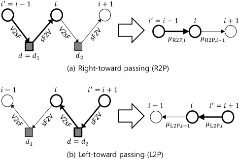
Figure 4: Graphical representation of the R2P/L2P update. This R2P/L2P update enables ssAMP-BGFD to exchange the adjacent information over the chain connection with $\mathcal{V}$ and $\mathcal{F}_{s}$, which is for seeking sparsity in the finite-difference $U_{d}=X_{i}-X_{i^{\prime}}$ where $i,i^{\prime}\in\mathcal{V}$ and $i,i^{\prime}\in ne(d)$.

The first key of this approach is to represent the residual,

$${r_{j}}={y_{j}}-\sum\nolimits_{i\in\mathcal{V}}{{h_{ji}}({\mu_{i}+{\Delta\mu_{i\to j}}})}\,\,\forall j\in\mathcal{F}_{m},$$ (38)

as a function of the non-directional parameters for the mF2V update. If done so, this will lead to a non-directional expression of $\rho_{i},\mu_{i}$ for the V2mF update. Namely, from (33b), we have

$${\rho_{i}} =\sum\nolimits_{j\in\mathcal{F}_{m}}{{h_{ji}}(\underbrace{{y_{j}}-\sum\nolimits_{i^{\prime}\in\mathcal{V}}{{h_{ji^{\prime}}}{\mu_{i^{\prime}\to j}}}}_{=r_{j}}+{h_{ji}}{\mu_{i\to j}})}$$

$$=\sum\nolimits_{j\in\mathcal{F}_{m}}{{h_{ji}}{r_{j}}}+\underbrace{\sum\nolimits_{j\in\mathcal{F}_{m}}{h_{ji}^{2}{\mu_{i\to j}}}}_{={\mu_{i}}(\text{as }M\to\infty)},$$ (39)

which is an input of (36) to generate $\mu_{i}$. The mF2V variance $\theta_{j\to i}$ becomes needless since by plugging (33d) in (34), we can obtain $\theta_{i}$ directly from the V2mF variance $\sigma_{i}^{2}$, i.e.,

$$\begin{array}[]{l}{\theta_{i}}=\Delta+\frac{1}{M}\sum\limits_{i^{\prime}\in\mathcal{V}}\underbrace{\sum\nolimits_{j\in\mathcal{F}_{m}}{h_{ji^{\prime}}^{2}\sigma_{i^{\prime}\to j}^{2}}}_{=\sigma_{i^{\prime}}^{2}(\text{as }M\to\infty)}-\underbrace{\sum\limits_{j\in\mathcal{F}_{m}}{h_{ji}^{2}\sigma_{i\to j}^{2}}}_{=\sigma_{i}^{2}(\text{as }M\to\infty)}\\ \,\,\mathop{=}\limits^{N\to\infty}\Delta+\frac{1}{M}\sum\nolimits_{i\in\mathcal{V}}{\sigma_{i}^{2}}\equiv\theta\end{array}$$ (42)

where we can drop the index $i\in\mathcal{V}$ from ${\theta}_{i}$ with $N\to\infty$. Instead of (42), we can use an approximation [15],[19]

$$\theta\approx\frac{1}{M}||\underline{r}||^{2}_{2}.$$ (43)

In this case, the variance estimation of ${\sigma_{i}^{2}}$ is also not necessary.

Then, the remaining is to obtain an non-directional expression of (38). We approach this through the two-step manipulation given below:

1. Applying the first-order approximation to the V2mF calculation, $\mu_{i\to j}=\eta(\rho_{i}+\Delta\rho_{i\to j};\theta_{i}+\Delta\theta_{i\to j})$,

2. Substituting the result of the first step to (38).

This approach has been introduced in [13]-[19],[21], where the authors verified that although approximation errors are induced in the manipulation, the errors are negligible with the large system limit ($N,M\to\infty$). We omit the details of the manipulation by referring the reader to the conventional literature [13]-[19],[21]. As a result, we obtain a non-directional expression of (38):

$$\begin{array}[]{l}{r_{j}}\mathop{=}\limits^{N,M\to\infty}{y_{j}}-{\sum\nolimits_{i}{h_{ji}}{\mu_{i}}+\underbrace{{r_{j}}\frac{N}{M}\left\langle{\eta^{\prime}(\rho_{i};\cdot)}\right\rangle}_{\text{Onsager term}}}.\end{array}$$ (45)

The last term of (45) corresponds to the term $\sum\nolimits_{i}{h_{ji}\Delta{\mu_{i\to j}}}$ of (38), which corrects the dependency on the index $j\in\mathcal{F}_{m}$ in the directional parameter $\mu_{i\to j}$. This correction term has been called Onsager term in the literature [13]-[19],[21] which is known as a key for convergence of the AMP iterations.

Algorithm 2 ssAMP-BGFD

Inputs: Measurements $\underline{y}$, a measurement matrix $\mathbf{H}$,

prior parameters $q,\sigma_{0}$

Initialization:

set $\{{\underline{\mu}},\underline{\sigma}^{2}\}^{(t=0)}=\{\underline{0},\underline{1}\sigma_{0}^{2}\}$, $\underline{r}^{(t=0)}=\underline{y}$

set $\{{\underline{\mu}_{\text{R2P}}},\underline{\sigma}_{\text{R2P}}^{2}\}^{(t=0)}=\{\underline{0},\underline{1}\sigma_{0}^{2}\}$, $\{{\underline{\mu}_{\text{L2P}}},\underline{\sigma}_{\text{L2P}}^{2}\}^{(t=0)}=\{\underline{0},\underline{1}\sigma_{0}^{2}\}$

Iteration:

for $t=1$ to $t^{*}$ do

    set ${\underline{\rho}^{(t)}}={{\mathbf{H}}^{T}}\underline{r}^{(t-1)}+\underline{\mu}^{(t-1)}$

    set $\theta^{(t)}=\Delta+\frac{1}{M}\underline{1}^{T}(\underline{\sigma}^{2})^{(t)}$

    set $\forall i\in\mathcal{V}\backslash\{1\}:$

$\begin{array}[]{l}\left\{\begin{gathered}{\mu_{{\text{R2P}},i}},\lx@algorithmicx@hfill\\ \sigma_{{\text{R2P}},i}^{2}\lx@algorithmicx@hfill\\ \end{gathered}\right\}^{(t)}\mathop{=}\left\{\begin{gathered}\phi({\rho_{i-1}^{(t)}};{\theta^{(t)}},\{{\mu_{{\text{R2P}},i-1}},\sigma_{{\text{R2P}},i-1}^{2}\}^{(t-1)}),\lx@algorithmicx@hfill\\ \zeta({\rho_{i-1}^{(t)}};{\theta^{(t)}},\{{\mu_{{\text{R2P}},i-1}},\sigma_{{\text{R2P}},i-1}^{2}\}^{(t-1)})\lx@algorithmicx@hfill\\ \end{gathered}\right\}\lx@algorithmicx@hfill\\ \end{array}$

    set $\forall i\in\mathcal{V}\backslash\{N\}:$

$\begin{array}[]{l}\left\{\begin{gathered}{\mu_{{\text{L2P}},i}},\lx@algorithmicx@hfill\\ \sigma_{{\text{L2P}},i}^{2}\lx@algorithmicx@hfill\\ \end{gathered}\right\}^{(t)}\mathop{=}\left\{\begin{gathered}\phi({\rho_{i+1}^{(t)}};{\theta^{(t)}},\{{\mu_{{\text{L2P}},i+1}},\sigma_{{\text{L2P}},i+1}^{2}\}^{(t-1)}),\lx@algorithmicx@hfill\\ \zeta({\rho_{i+1}^{(t)}};{\theta^{(t)}},\{{\mu_{{\text{L2P}},i+1}},\sigma_{{\text{L2P}},i+1}^{2}\}^{(t-1)})\lx@algorithmicx@hfill\\ \end{gathered}\right\}\end{array}$

    set $\underline{\mu}^{(t)}=\eta{({{\underline{\rho}}^{(t)}};\theta^{(t)},{\underline{\mu}_{\text{R2P}}},\underline{\sigma}_{\text{R2P}}^{2},{\underline{\mu}_{\text{L2P}}},\underline{\sigma}_{\text{L2P}}^{2})}$

    set $(\underline{\sigma}^{2})^{(t)}=\gamma{({{\underline{\rho}}^{(t)}};\theta^{(t)},{\underline{\mu}_{\text{R2P}}},\underline{\sigma}_{\text{R2P}}^{2},{\underline{\mu}_{\text{L2P}}},\underline{\sigma}_{\text{L2P}}^{2})}$

    $\begin{gathered}\text{set }\underline{r}^{(t)}=\underline{y}-{\mathbf{H}}\underline{\mu}^{(t)}\lx@algorithmicx@hfill\\ \,\,\,\,\,\,\,\,\,\,\,\,\,\,\,\,\,\,\,\,\,\,\,\,\,+\underline{r}^{(t-1)}\frac{N}{M}{\left\langle{\eta^{\prime}({\underline{\rho}}^{(t)};\theta^{(t)},{\underline{\mu}_{\text{R2P}}},\underline{\sigma}_{\text{R2P}}^{2},{\underline{\mu}_{\text{L2P}}},\underline{\sigma}_{\text{L2P}}^{2})}\right\rangle}\lx@algorithmicx@hfill\\ \end{gathered}$

end for

Outputs: $\widehat{\underline{x}}_{\text{ssAMP-1D}}=\underline{\mu}^{(t=t^{*})}$

III-C3 STEP III - Right/Left Toward Message-Passing at S-factors

In our factor graph model $\mathcal{G}(\mathcal{V},{\mathcal{F}_{m}},{\mathcal{F}_{s}})$, the edge connections between $\mathcal{V}$ and $\mathcal{F}_{s}$ are stronger than the connections between $\mathcal{V}$ and $\mathcal{F}_{m}$. This “weak/strong” concept is based on two facts:

• A s-factor $d\in\mathcal{F}_{s}$ has only two connections to $\mathcal{V}$; hence, the corresponding two scalars $X_{i},X_{i^{\prime}}$ ($i,i^{\prime}\in ne(d)$) have potentially larger influence on $d\in\mathcal{F}_{s}$ than a certain m-factor $j\in\mathcal{F}_{m}$ which has the other $N-2$ connections to $\mathcal{V}\backslash\{i,i^{\prime}\}$,

• The edge weight to $\mathcal{F}_{s}$ is relatively larger than the weight to $\mathcal{F}_{m}$: specifically, the edge weight to $\mathcal{F}_{s}$ is deterministically ‘1’, whereas the weight to $\mathcal{F}_{m}$ is imposed by the matrix entry $h_{ji}\in\mathbf{H}$ which is randomly distributed with zero-mean and the variance $\frac{1}{M}$.

For such strong edges, the approximation, given in the STEP II, does not hold [40]. Therefore, the sF2V and V2sF updates remains in the conventional sum-product form over the chain connection with $\mathcal{V}$ and $\mathcal{F}_{s}$.

Nevertheless, there is still room for the algorithm simplification. We note from (28) that the sF2V update $(d\to i)$ is simple assignment of the V2sF parameters $(i^{\prime}\to d)$ according to the direction of message-passing, where $i,i^{\prime}\in ne(d)$. This direction is decided by placement of the s-factor $d\in ne(i)$.

• When $d=d_{1}$ such that the s-factor is placed on the leftside of the variable node $i\in\mathcal{V}\backslash\{1\}$, we have $i^{\prime}=i-1$; hence, the sF2V parameters is toward right (see Fig.4-(a)).

• When $d=d_{2}$ such that the s-factor is on the rightside of the node $i\in\mathcal{V}\backslash\{N\}$, we have $i^{\prime}=i+1$; hence, the sF2V parameters is left-toward (see Fig.4-(b)).

Accordingly, what we only need is to keep track the V2sF update according to the direction of the sF2V message-passing. We combine these two updates by defining the Right/Left Toward Message-Passing (R2P/L2P) update as

$$\small\begin{array}[]{l}{\text{1) R2P}}\,{\text{update:}\hfill}\\ \forall i\in\mathcal{V}\backslash\{1\}\text{ and }i^{\prime}=i-1:\\ \left\{\begin{gathered}{\mu_{{\text{R2P}},i}},\hfill\\ \sigma_{{\text{R2P}},i}^{2}\hfill\\ \end{gathered}\right\}\equiv\left\{\begin{gathered}\mu_{i-1\to d},\hfill\\ \sigma_{i-1\to d}^{2}\hfill\\ \end{gathered}\right\}=\left\{\begin{gathered}\phi({\rho_{i-1}};{\theta},{\mu_{{\text{R2P}},i-1}},\sigma_{{\text{R2P}},i-1}^{2}),\hfill\\ \zeta({\rho_{i-1}};{\theta},{\mu_{{\text{R2P}},i-1}},\sigma_{{\text{R2P}},i-1}^{2})\hfill\\ \end{gathered}\right\},\hfill\\ \\ {\text{2) L2P}}\,{\text{update:}\hfill}\\ \forall i\in\mathcal{V}\backslash\{N\}\text{ and }i^{\prime}=i+1:\\ \left\{\begin{gathered}{\mu_{{\text{L2P}},i}},\hfill\\ \sigma_{{\text{L2P}},i}^{2}\hfill\\ \end{gathered}\right\}\equiv\left\{\begin{gathered}\mu_{i+1\to d},\hfill\\ \sigma_{i+1\to d}^{2}\hfill\\ \end{gathered}\right\}=\left\{\begin{gathered}\phi({\rho_{i+1}},{\theta};{\mu_{{\text{L2P}},i+1}},\sigma_{{\text{L2P}},i+1}^{2}),\hfill\\ \zeta({\rho_{i+1}},{\theta};{\mu_{{\text{L2P}},i+1}},\sigma_{{\text{L2P}},i+1}^{2})\hfill\\ \end{gathered}\right\},\end{array}$$ (71)

where without loss of generality, we set $\{{\mu_{\text{R2P},i=1}},\sigma_{\text{R2P},i=1}^{2}\}=\{{\mu_{\text{L2P},i=N}},\sigma_{\text{L2P},i=N}^{2}\}=\{0,\sigma_{0}^{2}\}$ for $i=1,N$. These R2P/L2P updates take a role of exchanging the neighboring information over the chain connection with $\mathcal{V}$ and $\mathcal{F}_{s}$, promoting the FD sparsity of $\underline{X}$. It is clarified from (71) that ssAMP-BGFD expends $\mathcal{O}(N)$ per-iteration cost for the R2P/L2P update.

III-D EM-Tuning of Prior Parameters

We provide an online-tuning strategy for the prior parameters, $\tau\equiv\{q,\sigma_{0}^{2}\}$ in ssAMP-BGFD. For this, we setup an maximum likelihood estimation (MLE), applying a popular technique, Expectation-Maximization (EM), to the estimation. This EM approach goes well with the Bayesian AMP parameter tuning, which has been demonstrated by Schniter et al. [17], Kamilov et al. [18], and Krzakala et al. [19] for the CS recovery problem with direct sparsity.

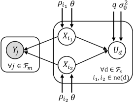
Figure 5: Graphical representation of the EM-tuning of the prior parameters $\mathbf{\tau}\equiv\{q,\sigma_{0}^{2}\}$

The statistical dependency in our MLE setup is graphically represented in Fig.5 where $X_{i_{1}},X_{i_{2}}$ and $\underline{Y}$ are related by the measurement model (1), and we know the connection $i_{1},i_{2}\in ne(d):U_{d}=X_{i_{2}}-X_{i_{1}}$ from (19). In this MLE, we consider the evidence PDF $f_{\underline{Y}}(\underline{y}|\tau)$ as the likelihood function. As in [44], we can decompose the log-likelihood into

$$\log f_{\underline{Y}}(\underline{y}|{\tau})=\mathcal{L}({\widehat{f}_{{\underline{U}}}},{\tau})+{\text{KL}}(\widehat{f}_{\underline{U}}||f_{{\underline{U}}|\underline{Y}})$$ (72)

for an arbitrary PDF ${\widehat{f}_{{\underline{U}}}}\equiv{\widehat{f}_{{\underline{U}}}}(\underline{u}|\tau)$, where we define two functionals, $\mathcal{L}(\cdot,{\tau}):V\to\mathbb{R}$, where $V\equiv\{\widehat{f}_{\underline{U}}:\mathbb{R}^{N}\to[0,1]\}$, and the Kullback-Leibler (KL) divergence ${\text{KL}}({\widehat{f}_{{\underline{U}}}}||f_{{\underline{U}}|\underline{Y}})$, as

$$\begin{gathered}\mathcal{L}({\widehat{f}_{{\underline{U}}}},{\tau})\equiv{\mathbb{E}_{{{\widehat{f}}_{{\underline{U}}}}}}[\log f_{\underline{Y},{\underline{U}}}(\underline{y},{\underline{u}}|{\tau})]+\mathbb{H}({\widehat{f}_{{\underline{U}}}})\hfill\\ \end{gathered},$$ (75)

$$\begin{gathered}{\text{KL}}({\widehat{f}_{{\underline{U}}}}||{f_{{\underline{U}}|\underline{Y}}})\equiv\mathbb{E}_{{\widehat{f}}_{{\underline{U}}}}\left[\log{\frac{{\widehat{f}_{{\underline{U}}}({\underline{u}}|\tau)}}{{f_{{\underline{U}}|\underline{Y}}({\underline{u}}|\underline{y},{\tau})}}}\right]\hfill\\ \end{gathered}.$$ (78)

Note in (72) that the lower bound, i.e., $\log{f_{\underline{Y}}}(\underline{y}|{\tau})\geq\mathcal{L}({\widehat{f}_{{\underline{U}}}},{\tau})$, holds true since the the KL divergence is non-negative.

The EM algorithm consists of two-stages for iteratively maximizing the log-likelihood (72). Let ${\tau^{t}}\equiv\{q,\sigma_{0}^{2}\}^{t}$ denote the current estimate of the parameter set. Then, we derive the EM update for the next estimate ${\tau^{t+1}}\equiv\{q,\sigma_{0}^{2}\}^{t+1}$ as follows.

TABLE I: List of recent solvers in the performance validation

Solvers	Optimization Setup	Parameter Tuning	Solver Type
ssAMP-BGFD	MMSE + BG prior	$q,\sigma_{0},\Delta$ (Oracle/EM)	Sum-product AMP
GrAMPA-BG [20]	MMSE + BG prior	$q,\sigma_{0},\Delta$ (Oracle)	Sum-product AMP (GAMP-based)
TVAMP [22]	MAP + Laplacian prior	$\lambda$ (Empirically optimal)	Max-sum AMP + FLSA [41] or Condat’s 1DTV [56]
EFLA [12]	TV method (2)	$\lambda$ (Empirically optimal)	First-Order + FLSA [41]
TV-CP [10]	TV method (2)	$\lambda$ (Empirically optimal)	First-Order + Chambolle-Pock [10]

III-D1 In the E-step

Given the current estimate ${\tau^{t}}$, we find the PDF ${\widehat{f}_{{\underline{U}}}}$ maximizing the lower bound $\mathcal{L}({\widehat{f}_{{\underline{U}}}},{\tau^{t}})$. For the optimum, we obviously need to set $\widehat{f}_{\underline{U}}=f_{{\underline{U}}|\underline{Y}}({\underline{u}}|\underline{y},{\tau}^{t})$ such that the KL divergence becomes zero and the log-likelihood achieves the lower bound, i.e., $\log{f_{\underline{Y}}}(\underline{y}|{\tau^{t}})=\mathcal{L}({\widehat{f}_{{\underline{U}}}},{\pi^{t}})$. The optimum PDF $\widehat{f}_{\underline{U}}$ is obtained by the product of marginal posterior of $U_{d}$. Namely, we have

$$\widehat{f}_{\underline{U}}=f_{{\underline{U}}|\underline{Y}}({\underline{u}}|\underline{y},{\tau})=\prod\nolimits_{d=1}^{N-1}{{f_{{U_{d}}|\underline{Y}}}({u_{d}}|\underline{y},{\tau})},$$ (79)

and then we find

$$\begin{gathered}{f_{U_{d}|\underline{Y}}}(u_{d}|\underline{y},{\tau})=\frac{{{f_{{U_{d}}}}({u_{d}}|\tau)\mathcal{N}(u_{d};{\rho_{i_{2}}}-{\rho_{i_{1}}},2\theta)}}{{\int{{f_{{U_{d}}}}({u_{d}}|\tau)\mathcal{N}(u_{d};{\rho_{i_{2}}}-{\rho_{i_{1}}},2\theta)d{u_{d}}}}}\hfill\\ \,\,\,\,\,\,\,\,\,\,\,\,\,\,\,\,\,\,\,\,\,\,\,\,\,\,\,\,\,\,\,\,\,\,\,\,\,\,\,=(1-{\pi_{d}})\delta({u_{d}})+{\pi_{d}}\mathcal{N}({u_{d}};{\gamma_{d}},\nu),\hfill\\ \end{gathered}$$ (83)

with some parameters definitions:

$$\begin{gathered}{\pi_{d}}\equiv\frac{1}{{1+{{{\frac{1-q}{{q}}\frac{\mathcal{N}(0;{\rho_{i2}}-{\rho_{i1}},2\theta)}{\mathcal{N}({\rho_{i_{2}}}-{\rho_{i_{1}}};0,2\theta+\sigma_{0}^{2})}}}}}}\hfill\\ \end{gathered},$$ (86)

$$\begin{gathered}{\gamma_{d}}\equiv\frac{{{{\rho_{i_{2}}}-{\rho_{i_{1}}}}}}{{\frac{2\theta}{{\sigma_{0}^{2}}}+1}}\hfill\\ \end{gathered},$$ (89)

$$\begin{gathered}\nu\equiv\frac{1}{{\frac{1}{{\sigma_{0}^{2}}}+\frac{1}{{2\theta}}}}\hfill\\ \end{gathered},$$ (92)

for $i_{1},i_{2}\in ne(d)$, where we note that $\rho_{i_{1}},\rho_{i_{2}},\theta$ are approximated by the ssAMP-BGFD iteration of Algorithm 2.

III-D2 In the M-step

We fix the PDF ${\widehat{f}_{{\underline{U}}}}$ by the E-step and maximize the lower bound $\mathcal{L}({\widehat{f}_{{\underline{U}}}},{\mathbf{\tau}^{t}})$ with respect to ${\mathbf{\tau}}$ to find an next estimate ${\mathbf{\tau}^{t+1}}$. Since the entropy term is independent of $\mathbf{\tau}$ in (75), this maximization clearly can be

$$\begin{gathered}{\tau^{t+1}}=\arg\mathop{\max}\limits_{\tau}{\mathbb{E}_{{{\widehat{f}}_{{\underline{U}}}}}}[\log f_{\underline{Y},\underline{U}}(\underline{y},{\underline{u}}|\mathbf{\tau}^{t})]\hfill\\ \,\,\,\,\,\,\,\,\,\,\,\,\,=\arg\mathop{\max}\limits_{\tau}\sum\limits_{d=1}^{N-1}{\mathbb{E}_{{{\widehat{f}}_{{U_{d}}}}}}[\log f_{U_{d}}(u_{d}|\mathbf{\tau}^{t})]\hfill\\ \end{gathered}$$ (96)

where the equality for the second line holds since we can express the joint PDF as $f_{\underline{Y},\underline{U}}(\underline{y},{\underline{u}}|\mathbf{\tau})=C\times\prod\nolimits_{d=1}^{N-1}{f_{U_{d}}}(u_{d}|\tau)$ for a $\tau$-independent term $C={f_{\underline{Y}|{\underline{X}}}}(\underline{y}|{\underline{x}})$.

The M-step maximization (96) need to be solved with respect to each parameter of $\tau$. We omit the detailed manipulation to handle this M-step maximization by referring readers to the work of Vila and Schniter (Section III-B of [17]). Finally, we formulate our EM update as:

$$\begin{gathered}{q^{t+1}}=\frac{1}{{N-1}}\sum\limits_{d=1}^{N-1}{\pi_{d}^{t}}\hfill\\ \end{gathered}$$ (99)

$$\begin{gathered}{(\sigma_{0}^{2})^{t+1}}=\frac{1}{{{q^{t+1}}(N-1)}}\sum\limits_{d=1}^{N-1}{{\pi_{d}}\left({|\gamma_{d}^{t}{|^{2}}+{\nu^{t}}}\right)}.\hfill\\ \end{gathered}$$ (102)

This EM-tuning routine can be optionally inserted at the end of the ssAMP-BGFD iteration. With (43), (99), and (102), ssAMP-BGFD can be parameter-free.

IV Performance Validation

In this section, we validate performance of the ssAMP-BGFD algorithm with extensive empirical results. Three types of experimental results will be discussed in this section:

1. Noiseless phase transitions,

2. Normalized MSE (NMSE) convergence over iterations,

3. Average CPU runtime.

All these experimental results were averaged using the Monte Carlo method with $100$ trials. At each Monte Carlo trial, we took a synthetic measurement vector $\underline{y}$ by realizing a signal $\underline{x}_{0}$, and an AWGN vector $\underline{w}$.

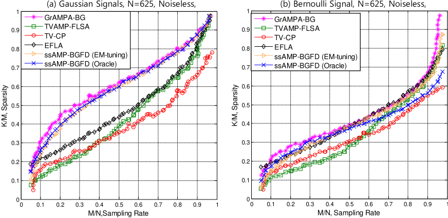
Figure 6: Empirical noiseless PT curves with std. Gaussian $\mathbf{H}$ for two types of the 1D piecewise-constant (PWC) signals: (a) Gaussian PWC signals and (b) Bernoulli PWC signals, which are generated by the PDFs given in Table II where we set the signal length $N=625$ and the variance $\sigma_{0}^{2}=1$.

In this experiment, we included recent solvers for the CS recovery with 1D-FD sparsity, listed in Table I, for a comparison purpose. The source codes of each solver was basically obtained from each authors’s webpage, but TV-CP and TVAMP were implemented by the authors. We provide two version of ssAMP-BGFD according to its EM option for the prior parameter learning. TVAMP was implemented in two ways: “TVAMP-FLSA” and “TVAMP-Condat” according to the denoiser implementation of (14). In addition, we configure GrAMPA to use the BG prior in this experiment, referring to the solver as “GrAMPA-BG” to specify its prior attribute.

We note that ssAMP-BGFD and GrAMPA-BG were configured by the oracle-tuning for the prior parameter $q,\sigma_{0}$ and the noise variance $\Delta$, but ssAMP-BGFD could be parameter-free with the EM-tuning (discussed in Section III-D). For TV-AMP, EFLA, and TV-CP, we used an empirically optimal $\lambda$ for each ($\frac{K}{M},\frac{M}{N}$). Finally, we set the initial guess of the signal estimate to a zero vector for all the solvers. For your information, we note that the empirical results, reported in this paper, have some changes from the results given in our conference paper [24] due to some mis-configuration corrections.

IV-A Noiseless Phase Transition

IV-A1 Experimental setup

For each PT curve, we basically considered a $38\times 38$ grid where we uniformly divided the range $\frac{M}{N}\in[0.05,0.99]$ as the x-axis and the range $\frac{K}{M}\in[0.05,0.99]$ as the y-axis with the stepsize $0.025$. A PT curve is connection of experimental points having 0.5 success rate of the signal recovery, where the recovery success is declared when $\text{NMSE}\equiv\frac{{||{{\underline{x}}_{0}}-\underline{\widehat{x}}||_{2}^{2}}}{{||{{\underline{x}}_{0}}||_{2}^{2}}}\leq 10^{-4}$. We set the number of maximum iterations to $t^{*}=2000$, and the iteration stopping tolerance was very tightly set to $\frac{{||{{\underline{\mu}}^{(t)}}-{{\underline{\mu}}^{(t+1)}}||_{2}^{2}}}{{||{{\underline{\mu}}^{(t)}}||_{2}^{2}}}\leq\text{tol}=10^{-14}$; hence, the PT curves are supposed to represent algorithm performance after convergence.

IV-A2 Comparison over the other solvers

In Fig.6, we provide a PT comparison over the recent solvers listed in Table I. For this, we fixed $\mathbf{H}$ to the standard Gaussian matrix whose entries are drawn from $\mathcal{N}(h_{ji};0,\frac{1}{M})$, setting to $N=625$. Then, we draw PT curves for two types of the signal statistics given in Table II.

In the Gaussian case, we observe from Fig.6-(a) that GrAMPA-BG provides the state-of-the-art, and ssAMP-BGFD retains its place very close to GrAMPA-BG. Those two algorithms significantly improve on the PT performance of the others because their BG prior has a very good match with the Gaussian statistics. We also note in the Gaussian case that the EM method exactly tunes the prior parameters of ssAMP-BGFD such that its PT curve coincides with that by the oracle tuning.

For the Bernoulli case, Fig.6-(b) reports that ssAMP-BGFD using EM is the closest to GrAMPA-BG together with EFLA, and better than TV-CP and TVAMP-FLSA even though its advantage is less remarkable compared to the Gaussian case. In this case, the oracle tuning of ssAMP-BGFD is not as fine as in the Gaussian case because the BG prior is not basically able to provide an accurate description to the statistic of the Bernoulli PWC.

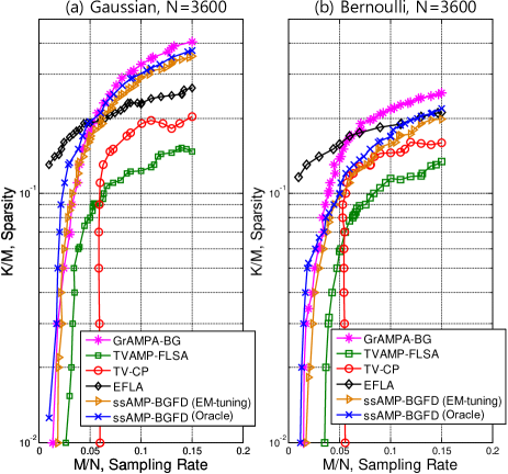
Figure 7: Empirical noiseless PT curves with std. Gaussian $\mathbf{H}$ for the case of $M\ll N$ with $N=3600$.

To better understand the PT characteristic when small $M/N$ ($M\ll N$), we fixed $N=3600$ and constructed a $22\times 8$ uniform grid of ($\frac{K}{M},\frac{M}{N}$) with the stepsize $0.02$ where the range of the x-axis is $\frac{M}{N}\in[0.01,0.15]$, and the range of the y-axis is $\frac{K}{M}\in[0.01,0.43]$. We observe from Fig.7 that as $M/N\to 0$, the PT curves of ssAMP-BGFD and GrAMPA-BG becomes nearly identical, worse than that of EFLA, and much better than those of TVAMP-FLSA and TV-CP.

These comparison results support that ssAMP-BGFD shows the PT performance closely approaching the state-of-the-art by GrAMPA-BG, being superior to the others.

TABLE II: Statistics of the 1D-PWC signals $\underline{X}$

Type	Signal PDFs, $f_{U_{d}}(u_{d})$
Gaussian PWC	$(1-q)\delta(u_{d})+q\mathcal{N}(u_{d};0,\sigma_{0}^{2})$
Bernoulli PWC	$(1-q)\delta(u_{d})+q\mathcal{U}(u_{d}\in\{-{\sigma_{0}},{\sigma_{0}}\};\frac{1}{2})$

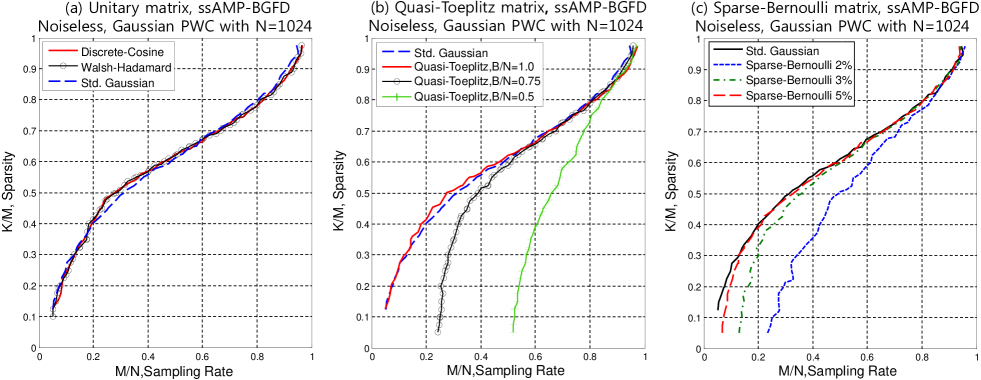
Figure 8: Empirical noiseless PT curves of ssAMP-BGFD (with the EM-tuning) working with non-i.i.d.-random $\mathbf{H}$ and column-sign-randomization: (a) sub-sampled unitary matrices (DCT and WHT), (b) quasi-Toeplitz matrices with the damping factor $\beta=0.5$, (c) sparse-Bernoulli matrices for a variety of the matrix sparsity, where we consider Gaussian PWC signal with $N=1024$.

IV-A3 PT curve of ssAMP-BGFD with RIP matrices $\mathbf{H}$

Candes et al. discussed a natural property on the measurement matrix $\mathbf{H}$ (abbreviated by D-RIP), which is a variant of the restricted isometry property (RIP) for the analysis CS setup [48]. Then, they also stated using the result of [49] that any $\mathbf{H}$ satisfying the standard RIP requirement, will also satisfy the D-RIP with “column-sign-randomization”. Specifically, instead of (1), we consider the measurement generation:

$$\underline{Y}=\underbrace{\mathbf{H}}_{{\text{RIP matrix}}}{\text{diag}}(\underbrace{[1,1,-1,1...,-1]}_{N{\text{ independent random signs}}})\,\underline{X}+\underline{W}.$$ (103)

This leads us to test practical RIP matrices for the proposed algorithm, such as unitary matrices, quasi-Toepliz matrices and/or deterministic matrices, which aims to overcome the practical limitation of AMP (discussed in Section II). We refer the reader to [49] for specific RIP condition of each matrix listed above. In this experiment, we demonstrate that ssAMP-BGFD works well with such RIP matrices and the column-sign-randomization by showing empirical evidences for the Gaussian PWC signals with $N=1024$.

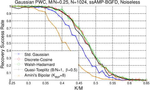
Figure 9: Empirical PT comparison of ssAMP-BGFD (EM-tuning) with various types of the matrices $\mathbf{H}$: Amini’s deterministic bipolar matrix ($K_{\text{RIP}}=8$) [61], DCT and WHT matrices, a quasi-Toeplitz matrix $(B/N=1.0)$ with damping ($\beta=0.5$), and the std. Gaussian matrix, where we consider $M/N=0.25$ and Gaussian PWC with $N=1024$.

• With sub-sampled unitary matrices: We test the two unitary systems: Discrete Cosine Transform (DCT) and Walsh-Hadamard Transform (WHT) with ssAMP-BGFD. We construct $\mathbf{H}$ by randomly sampling $M$ rows from the $N\times N$ DCT or WHT matrix. For such matrices $\mathbf{H}$, the complexity of the matrix-vector multiplication can be reduced to $\mathcal{O}(N\log N)$ from $\mathcal{O}(MN)$ via the fast DCT/WHT method. Fig.8-(a) shows that the PT curve of the DCT and WHT matrices coincides with that of the standard Gaussian matrix.

• With quasi-Toeplitz matrices with damping: We consider quasi-Toeplitz $\mathbf{H}$ for ssAMP-BGFD: the first row consists of $B$ zero-mean Gaussian coefficients, and each row of $\mathbf{H}$ is a copy of the first row with cyclic permutation [50],[51]. This matrix requires memory storage only for the $B$ random numbers, enabling fast matrix-vector multiplications using the FFT method ($\mathcal{O}(N\log N)$ complexity). In addition, the row sampling of $\mathbf{H}$ need not be random in contrast to the unitary case. On the other hand, in this case, the columns of $\mathbf{H}$ are severely correlated, and it may lead to the AMP divergence. For this, we use a simple damping method to stabilize the ssAMP-BGFD iteration. Namely, for the residual update, we use

  $$\small\begin{array}[]{l}\small{\underline{r}^{(t)}}=(1-\beta){\underline{r}^{(t-1)}}+\beta\left({\underline{y}-{\mathbf{H}}{{\underline{\mu}}^{(t)}}+{{\underline{r}}^{(t-1)}}\frac{N}{M}\left\langle{\eta^{\prime}(\cdot)}\right\rangle}\right)\end{array}$$ (105)

  where $0<\beta\leq 1$ is the damping factor. As shown in Fig.8-(b), we test the quasi-Toeplitz matrices for three cases , $B/N=0.5$, $B/N=0.75$ and $B/N=1.0$ with the damping factors $\beta=0.5$.

• With deterministic matrices: Several deterministic construction of $\mathbf{H}$ have been developed to overcome some drawbacks of the random $\mathbf{H}$ [60],[61]: mainly, there are no efficient methods to verify whether a specific realization of the random $\mathbf{H}$ meets the RIP requirement. DeVore provided a deterministic construction of cyclic binary $\mathbf{H}\in\{0,1\}^{M\times N}$ satisfying the RIP under some conditions [60]. Then, Amini et al. made a connection between the DeVore’s approach and channel coding theory (specifically BCH codes) and suggesting construction of cyclic bipolar $\mathbf{H}\in\{-1,1\}^{M\times N}$ [61]. One disadvantage of such deterministic $\mathbf{H}$ is that the matrix size $(M,N)$ is restricted by the code length. Under the ssAMP-BGFD recovery, we compare a PT curves by the $255\times 1024$ Amini’s matrix satisfying RIP order of $K_{\text{RIP}}=8$, to PT curves by the $256\times 1024$ matrices considered above. Fig.9 shows that Amini’s matrix works well with ssAMP-BGFD even through its PT curve slightly underperforms the PT curve by the other matrices.

IV-A4 PT curve of ssAMP-BGFD with matrix sparsity

We consider the use of sparse matrices with ssAMP-BGFD. This is motivated by Low-Density Parity-Check (LDPC) codes as the works in [36]-[38],[46]. The use of the sparse $\mathbf{H}$ provides an accelerated fast matrix-vector multiplication method (its complexity is proportional to the number of nonzeros in $\mathbf{H}$), requiring small memory to store the matrix entries. We examine sparse-Bernoulli random $\mathbf{H}\in\{0,-1,1\}^{M\times N}$ whose column weight is fixed to $L$ such that the matrix sparsity is $L/M\times 100$. Fig.8-(c) reports the corresponding PT curves for a variety of the matrix sparsity: 2,3, and 5% sparsity.

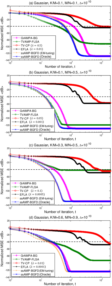
Figure 10: NMSE convergence over iterations for the four cases of ($\frac{K}{M},\frac{M}{N}$) where Gaussian PWC signals are with $N=3600$ and $\sigma_{0}^{2}=1$; the noise variance is set to $\Delta=10^{-10}$; the matrix $\mathbf{H}$ is set to the std. Gaussian.

IV-B NMSE Convergence over Iterations

IV-B1 Experimental setup

We measured NMSE over iterations for the four different cases of ($\frac{K}{M},\frac{M}{N}$):

• Case (a) - $\frac{K}{M}=0.1,\frac{M}{N}=0.1$,

• Case (b) - $\frac{K}{M}=0.1,\frac{M}{N}=0.5$,

• Case (c) - $\frac{K}{M}=0.3,\frac{M}{N}=0.5$,

• Case (d) - $\frac{K}{M}=0.6,\frac{M}{N}=0.9$,

which are points satisfying the Gaussian PT curve of all the solvers (see Fig.6-(a)). In this experiment, we set the noise variance to $\Delta=10^{-10}$, the signal length to $N=3600$, and consider the standard Gaussian $\mathbf{H}$. Also, we inform that all the solvers were set to run by $t^{*}=2000$ iterations without any stopping criterion.

IV-B2 Discussion for the Gaussian PWC case

We consider the Gaussian PWC case first. Table IV and Fig.10 reports that in all the cases, ssAMP-BGFD converges remarkably faster than EFLA and TV-CP, being advantageous over TVAMP-FLSA and GrAMPA-BG. Although TVAMP-FLSA shows the fastest convergence rate in the case (a), it pales into insignificance due to an non-negligible NMSE gap from ssAMP-BGFD at the fixed-point. In such a aspect, GrAMPA-BG is the most comparable, but there exists an uniform gap between ssAMP-BGFD and GrAMPA-BG in convergence rate. We state that this gap is caused by difference of the sF2V message modeling methods (discussed in Section III-C). We support our statement by plotting empirical PDFs of the estimated Gaussian PWC at iteration $t=20$, as shown in Fig.11. In case (b), GrAMPA-BG’s method induces approximation errors in the sF2V modeling, delaying its convergence, resulting in an empirical PDF with a blunt peak at $t=20$. In contrast, ssAMP-BGFD’s method does not cause such errors, promoting its convergence, showing a sharp PDF whose peak nearly coincides with that of the prior PDF even at $t=20$. We also note from Fig.11 that in the case (d), ssAMP-BGFD requires far more iteration than $t=20$ for its convergence, implicating that its convergence advantage is decayed compared to the case (b). This is because the BG-based modeling method of ssAMP-BGFD, given in (28), less effective for non-sparse signals having high $K/M$.

IV-B3 Discussion for the Bernoulli PWC case

In the Bernoulli PWC case, every algorithm basically requires more iterations than the Gaussian case. In addition, we observe from Table IV that in the case (d), the oracle ssAMP-BGFD does not achieve the NMSE =-40dB whereas ssAMP-BGFD with EM does. This observation implicates that the EM-tuning effectively assists ssAMP-BGFD to estimate the Bernoulli PWC signals using the BG prior. This is also connected to the PT improvement of ssAMP-BGFD in Fig.6-(b).

TABLE III: The average number of iterations for achieving the normalized MSE = -40 dB where $N=3600,\Delta=10^{-10}$, and Gaussian PWC.

	Case (a)	Case (b)	Case (c)	Case (d)
Algorithms	K/M=0.1,	K/M=0.1,	K/M=0.3,	K/M=0.6,
	M/N=0.1	M/N=0.5	M/N=0.5	M/N=0.9
ssAMP-BGFD	60	$\mathbf{14}$	17	25
(Oracle)
ssAMP-BGFD	66	$\mathbf{14}$	$\mathbf{16}$	$\mathbf{17}$
(EM-tuning)
TV-CP	921	515	823	1525
EFLA	228	192	289	335
TVAMP-FLSA	$\mathbf{36}$	$\mathbf{14}$	39	23
GrAMPA-BG	121	24	28	20

TABLE IV: The average number of iterations for achieving the normalized MSE = -40 dB where $N=3600,\Delta=10^{-10}$, and Bernoulli PWC.

	Case (a)	Case (b)	Case (c)	Case (d)
Algorithms	K/M=0.1,	K/M=0.1,	K/M=0.3,	K/M=0.6,
	M/N=0.1	M/N=0.5	M/N=0.5	M/N=0.9
ssAMP-BGFD	66	$16$	$\mathbf{25}$	$\infty$
(Oracle)
ssAMP-BGFD	75	$\mathbf{14}$	28	$\mathbf{44}$
(EM-tuning)
TV-CP	1044	570	$\infty$	$\infty$
EFLA	234	191	324	494
TVAMP-FLSA	$\mathbf{54}$	15	$\infty$	69
GrAMPA-BG	143	25	39	47

IV-C Average CPU Runtime

In order to clarify the computational advantage of ssAMP-BGFD, we provide a comparison of CPU runtime over the algorithms of Table I.

IV-C1 Experimental setup

In this experiment, we again considered the four cases of ($\frac{K}{M},\frac{M}{N}$) given in Section IV-B, the Gaussian PWC, the noise variance $\Delta=10^{-10}$, and the standard Gaussian $\mathbf{H}$. For a fair comparison, we set a target MSE since some algorithms may run longer but give a better MSE without any stopping criterion. Namely, we made all the algorithms to stop their iterations when reaching the target MSE $\frac{{||{{\underline{x}}_{0}}-\underline{\widehat{x}}||_{2}^{2}}}{{||{{\underline{x}}_{0}}||_{2}^{2}}}\leq 10^{-4}$ ($-40$ dB of NMSE). We loosely set the maximum iterations to $t^{*}=2000$ based on the result of Section IV-B. In addition, we only counted the cases where all the algorithm achieve the target MSE. We inform that this runtime measuring was performed by using the “tic-and-toc” functions of MATLAB R2013b with Intel Core i7-3770 CPU (3.40 GHz) and RAM 24GB. Finally, we clarify that the 1D-FD matrix $\mathbf{D}$ for GrAMPA-BG and TV-CP is declared by the “sparse” attribute in MATLAB.

IV-C2 Discussion

The complexity cost of the algorithms are dominated by the matrix-vector multiplications, i.e., $\mathbf{H}\underline{\mu}$ and $\mathbf{H}^{T}\underline{r}$. In the case of ssAMP-BGFD and TVAMPs, their per-iteration cost is straightforwardly $\mathcal{O}(MN)$ since they include $\mathbf{H}\underline{\mu}$ and $\mathbf{H}^{T}\underline{r}$ once in a lap of the iteration. EFLA is also $\mathcal{O}(MN)$ by including variably 2$\sim$3 times of the multiplications per iteration. For TV-CP and GrAMPA-BG, their cost is naively $\mathcal{O}(N^{2})$ due to the size of the 1D-FD operator $\mathbf{D}\in\mathbb{R}^{N\times N-1}$, but the cost can be reduced to $\mathcal{O}(MN)$ by applying a fast sparse matrix multiplication method. In Fig.12, we take notice slopes of the runtime curves which manifest the complexity cost. Since the rate $M/N$ is fixed for each case, the per-iteration cost $\mathcal{O}(MN)$ becomes $\mathcal{O}(N^{2})$; hence all the curves approximately have slope ‘2’ with sufficiently large $N$ when the x-axis plot the length $N$ on a logarithmic scale.

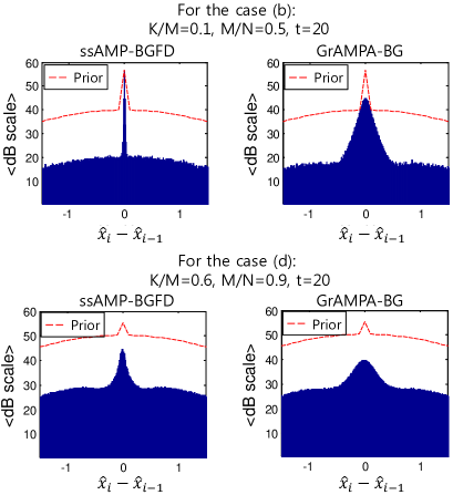
Figure 11: Empirical PDFs (in dB scale) of the estimated Gaussian PWC by ssAMP-BGFD (w/ the EM-tuning) and GrAMPA-BG. These data were obtained with $N=10^{5}$, $\sigma_{0}^{2}=1$, $\Delta=10^{-10}$, and iteration $t=20$ for the two cases: Case (b) ($\frac{K}{M}=0.1$, $\frac{M}{N}=0.5$) and Case (d) ($\frac{K}{M}=0.6$, $\frac{M}{N}=0.9$)

TABLE V: Average CPU runtime (in seconds) per iteration $(N=10000,\Delta=10^{-10})$, Gaussian PWC signals (by MATLAB R2013b with Intel Core i7-3770 CPU (3.40 GHz) with RAM 24GB)

Algorithms	(a) K/M=0.1, M/N=0.1	(b) K/M=0.1, M/N=0.5	(c) K/M=0.3, M/N=0.5	(d) K/M=0.6, M/N=0.9
ssAMP-BGFD (Oracle)	0.014$\pm$4.9e-4	0.052 $\pm$ 1.3e-3	0.050$\pm$1.1e-3	0.094$\pm$3.2e-3
ssAMP-BGFD (EM-tuning)	0.012$\pm$5.4e-4	0.050 $\pm$ 2.0e-3	0.049$\pm$2.2e-3	0.090$\pm$2.7e-2
TV-CP	0.011$\pm$4.5e-4	0.049 $\pm$ 7.0e-4	0.049$\pm$7.1e-4	0.088$\pm$1.8e-2
EFLA	0.017$\pm$2.8e-3	0.063 $\pm$ 9.6e-3	0.062$\pm$9.7e-3	0.128$\pm$5.1e-2
TVAMP-FLSA	0.027$\pm$1.3e-3	0.055 $\pm$ 2.0e-3	0.054$\pm$1.8e-3	0.081$\pm$2.0e-3
TVAMP-Condat	0.010$\pm$3.3e-4	0.038 $\pm$ 1.2e-3	0.038$\pm$1.0e-3	0.066$\pm$1.6e-3
GrAMPA-BG	0.012$\pm$4.8e-4	0.051 $\pm$ 3.8e-3	0.052$\pm$5.4e-3	0.092$\pm$3.8e-2

Then, what are the factors distinguishing the superiority of the runtime curves in this comparison? The most dominant one is the convergence speed discussed in Section IV-B, which determines the required number of iterations to achieve the target MSE$=10^{-4}$ (see Table IV and IV). Therefore, this mainly decides the order of the runtime curves in Fig.12. The second factor is the per-iteration runtime of the algorithms given in Table V, corresponding to the number of the matrix-vector multiplications per iteration. Therefore, we can approximately calculate

CPU runtime

$$\approx{\text{ (\# of iteration to Target MSE) }}\times{\text{ (Per-iteration cost).}}$$

In some cases, the second factor highly accelerates the recovery. In this regard, TVAMP-Condat is very competitive because it has the smallest second factor. In all the cases of Fig.10, it is observed that TVAMP-Condat moves up its runtime from that of TVAMP-FLSA by its cheap per-iteration cost. This also verifies our argument in Section II-A that TVAMP can have very good scalability for large $N$ according to choice of the numerical implementation methods of (14).

Figure 12: CPU runtime comparison (in seconds) over signal length $N$ for the four cases of ($\frac{K}{M}$, $\frac{M}{N}$), where we consider the Gaussian PWC signals $\underline{X}$, the noise variance $\Delta=10^{-10}$, and target MSE $\frac{{||{{\underline{x}}_{0}}-\underline{\widehat{x}}||_{2}^{2}}}{{||{{\underline{x}}_{0}}||_{2}^{2}}}\leq 10^{-4}$. The matrix $\mathbf{H}$ is set to the std. Gaussian. We used MATLAB with Intel Core i7-3770 CPU (3.40 GHz) with RAM 24GB for this experiment.

This runtime comparison validates the low-computationality of ssAMP-BGFD. Its fast convergence nature and cheap per-iteration cost provides a generally faster solution to all the cases of Fig.10. In the case (a), although ssAMP-BGFD hands over the lead to TVAMP-Condat, it is still far better than TV-CP and EFLA, being advantageous over TVAMP-FLSA and GrAMPA-BG. In addition, the result of Section IV-B (see Fig.10-(a)) implicates that ssAMP-BGFD can be faster than TVAMP-Condat if the target MSE is finer.

V Practical Example: Compressed Sensing Recovery of SNP Genomic Data

V-A Background

In this section, we examine the ssAMP-BGFD algorithm to the CS recovery of genomic data. In this example, we consider a real data set of single nucleotide polymorphism (SNP) arrays which is a data measure for DNA copy numbers of genomic region. The SNP data shows a 1D-PWC pattern with FD sparsity when gene mutations occur. Specifically, the mutation causes a gene to be either deleted from the chromosome or amplified, leading to contiguous variation of the DNA copy numbers. Therefore, we can identify some diseases like cancers by analyzing the SNP pattern variation. Such a measured SNP data has been manually interpreted by biologists, but this is time-consuming and inaccurate for two natures of the genomic data: 1) the huge datasize and 2) severe noise. Hence, in recent years, DSP approaches have got attention for automatic interpretations of the genomic data, providing improved accuracy of the analysis [1],[2]. The CS framework is one line of such DSP approaches, which can resolve the datasize problem (by measurement sampling with dimensionality reduction) and the denoising problem (by sparsity regularization) simultaneously.

V-B Experimental setup

We provide a simple demonstration of the CS framework to the SNP data set. This data set was picked from the chromosome 7 region of glioblastoma multiforme (GBM) tumor, which has a large degree of copy number variation. From the data set, we used the 28th, 41th, 78th, and 124th SNP samples for this demonstration. First, we generated CS measurements $\underline{Y}$ from the noisy samples $\underline{X}$ using the standard Gaussian matrix $\mathbf{H}$ with $M/N=0.5$, then applying an algorithms to reconstruct the denoised samples $\widehat{\underline{X}}$ from $\underline{Y}$, where we tested some algorithms from Table I: ssAMP-BGFD (Proposed, w/o the EM-tuning), TVAMP-Condat [22],[56], TV-CP [10] and GrAMPA-BG [20]. We cannot optimally calibrate the parameters of these tested algorithms because this example is data-driven; namely, there are no reference signals for the recovery. Instead, we heuristically configured each algorithm with the parameters minimizing $l_{1}$-norm of the denoised sample $\widehat{\underline{X}}$, where we fixed $\sigma_{0}=1$ and restricted the scope of the parameters to $q\in\{10^{-6},10^{-5},10^{-4},10^{-3},10^{-2}\},\Delta\in[0.01,1.0],\lambda\in\{0.01,0.1,1,10\}$. We set $\text{tol}=10^{-8}$ and $t^{*}=2000$.

V-C Discussion

As shown in Fig.13, all of the algorithms successfully recognize 1D-PWC patterns indicating the copy number alternations in the gene samples $\widehat{\underline{X}}$. TVAMP-Condat appears to be the most practical algorithm for this SNP demonstration because of its fastest CPU runtime and its powerful denoising ability. GrAMPA-BG has the best denoising ability but its slow CPU runtime is demanding in practice. The TV-CP curves do not catch the PWC shape of the SNP samples, which might cause misidentification of copy number variations if the samples are severely noisy. The proposed ssAMP-BGFD shows clean PWC patterns with reasonable CPU runtime for all the SNP samples.

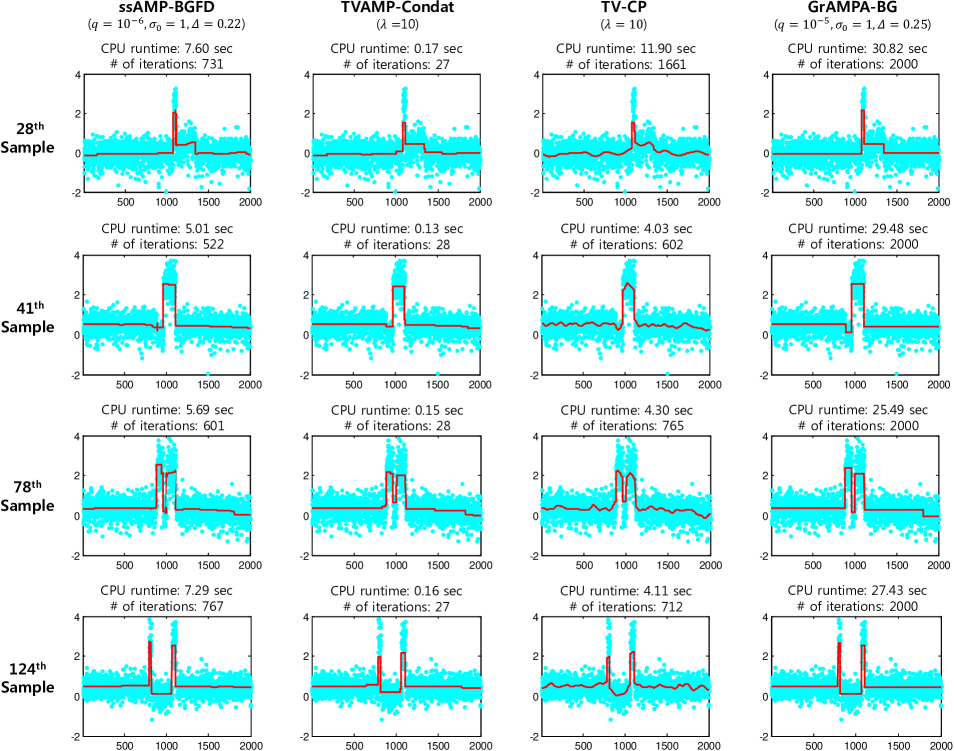
Figure 13: An exemplary demonstration of the CS recovery ($M/N=0.5$) with FD sparsity to five SNP samples of the chromosome 7 region of GBM tumor cell. Panels in the same row are for the same SNP sample. The blue-dots in each panel represents the original noisy SNP sample $\underline{X}$. The red-solid line in each panel indicates the SNP sample $\widehat{\underline{X}}$ reconstructed and denoised from the CS measurements $\underline{Y}=\mathbf{H}\underline{X}$ via a certain algorithm, whose name is shown on the top of each column with its parameter setup, where we use the standard Gaussian $\mathbf{H}$. In addition, we provide CPU runtime (in sec) spent by each reconstruction on the top of each panel where we used MATLAB R2013b with Intel Core i5-750 CPU (2.67 GHz) with RAM 18GB for the CPU runtime measuring.

VI Conclusions and Further works

The ssAMP-BGFD algorithm, which has been proposed in the present work, aims to solve the CS recovery with 1D-FD sparsity in terms of MMSE estimation (6). In this paper, the algorithm construction of ssAMP-BGFD has been mainly discussed. We have emphasized that the key of this construction is a sum-product rule, given in Algorithm 1, based on a factor graph consisting of two types of the factor nodes: the “s-factors” describing the finite-difference (FD) connection of the signal $\underline{X}$, and the “m-factors” being associated with the measurement generation (1). From a Bayesian prospective, we have imposed a Bernoulli-Gaussian prior (19) on the s-factors, seeking the FD sparsity of $\underline{X}$. Then, we have shown the derivation of ssAMP-BGFD from the sum-product rule, where the Gaussian approximation based on the central-limit-theorem and the first-order approximation were applied to the message update with the m-factors, and a proposed method was used to simplify the message update with the s-factors. In addition, we have provided an EM-tuning methodology for the prior parameter learning. The operations of ssAMP-BGFD is fully scalar-separable and low-computational. In addition, ssAMP-BGFD can be parameter-free with the EM-tuning, showing phase transition closely approaching the state-of-the-art performance by recent algorithms. We have empirically validated these characteristics of ssAMP-BGFD compared to the algorithms listed in Table I. As a practical example, we have applied the ssAMP-BGFD algorithm to the compressed sensing framework with SNP genomic data set, demonstrating that ssAMP-BGFD works well with real-world signals. An important further work is 2D/3D extension of the ssAMP-BGFD algorithm. This work is very essential in order to apply the ssAMP-BGFD algorithm to image denoising applications.

References

- [1] D. Witten and R. Tibshirani, “Extensions of sparse canonical correlation analysis with applications to genomic data,” Stat. Appl. Genet. Mol. Biol., vol. 8, issue 1, article no. 28, 2009.
- [2] D. Witten, R. Tibshirani, and T. Hastie, “A penalized matrix decomposition, with applications to sparse principal components and canonical correlation analysis,” Biostatistics, vol 10, issue 3, pp. 515-534, Apr. 2009.
- [3] M.A. Little, and NS. Jones. “Sparse Bayesian step-filtering for high-throughput analysis of molecular machine dynamics,” Proc. of IEEE ICASSP Conf., pp. 4162-4165, Dallas, TX, Mar. 2007.
- [4] Y. Sowa, A. Rowe, M. Leake, T. Yakushi, M. Homma, A. Ishijima, and R. Berry, “Direct observation of steps in rotation of the bacterial flagellar motor,” Nature, vol. 437, no. 7060, pp. 916-919, 2005.
- [5] M.A. Little and N.S. Jones, “Generalized methods and solvers for noise removal from piecewise constant signals: I. Background theory,” Proc. of the Royal Society of London A: mathematical, physical and engineering sciences, vol. 467, no. 2135, pp. 3088-3114, Nov. 2011.
- [6] L.I. Rudin, S. Osher, and E. Fatemi, “Nonlinear total variation based noise removal algorithms,” Physica D:Nonlinear Phenomena, vol. 60, pp. 259-268, Nov. 1992.
- [7] S.S. Chen, D.L. Donoho, and M.A. Saunders, “Atomic decomposition by basis pursuit,” SIMA J. Sci. Comput., vol 20, issue 1, pp. 33-61, 1998
- [8] E.J. Candes, J. Romberg, and T. Tao, “Robust uncertainty principles: Exact signal reconstruction from highly incomplete frequency information,” IEEE Trans. Inf. Theory., vol. 52, no. 2, pp. 489-509, Feb. 2006
- [9] R. Tibshirani, M. Saunders, S. Rosset, J. Zhu, and K. Knight, “Sparsity and smoothness via the fused lasso,” J. R. Statist. Soc. Ser. B, vol.67, no. 205, pp. 91-108, 2005.
- [10] A. Chambolle, T. Pock, “A first-order primal-dual algorithm for convex problems with applications to imaging,” J. Math. Imag. Vis., vol. 40, pp. 120-145, May 2011.
- [11] A. Beck, and M. Teboulle. “A fast iterative shrinkage-thresholding algorithm for linear inverse problems,” SIAM J. on Imag. Sci., vol. 2, no. 1, pp. 183-202, 2009.
- [12] J. Liu, L. Yuan, and J. Ye, “An efficient algorithm for a class of fused lasso problems,” proc of ACM SIGKDD Conference on Knowledge Discovery and Data Mining, 2010.
- [13] D.L. Donoho, A. Maleki, and A. Montanari, “Message passing algorithms for compressed sensing,” Proc. Nat. Acad. Sci., vol. 106, pp. 18914-18919, Nov. 2009.
- [14] D.L. Donoho, A. Maleki, and A. Montanari, “Message passing algorithms for compressed sensing: I. Motivation and construction,” Proc. in IEEE Inform. Theory Workshop (ITW), Cairo, Egypt, Jan. 2010.
- [15] A. Montanari, “Graphical models concepts in compressed sensing,” available at arXiv:1011.4328v3[cs.IT], Mar. 2011.
- [16] S. Rangan, “Generalized approximate message passing for estimation with random linear mixing,” available at ArXiv:1010.5141v2 [cs.IT], Aug. 2012.
- [17] J. Vila and P. Schniter, “Expectation-maximization Gaussian-mixture approximate message passing,” IEEE Trans. Signal Process., vol. 61, no. 19, pp. 4658-4672, Oct. 2013.
- [18] U.S. Kamilov, S. Rangan, A. K. Fletcher, and M. Unser, “Approximate message passing with consistent parameter estimation and applications to sparse learning,” IEEE Trans. Inform. Theory., vol. 60, no. 5, pp. 2969-2985, May 2014.
- [19] F. Krzakala, M. Mezard, F. Sausset, Y. Sun, and L. Zdeborova, “Statistical physics-based reconstruction in compressed sensing,” Phys. Rev X, No. 021005, May 2012.
- [20] M.A. Borgerding, P. Schniter, J. Vila, and S. Rangan, “Generalized approximate message passing for cosparse analysis vompressive sensing,” Proc. IEEE Conf. on Acoustics Speech and Signal Processing (ICASSP), (Brisbane, Australia), Apr. 2015. MATLAB code is available at http://www2.ece.ohio-state.edu/ schniter/GrAMPA/index.html.
- [21] M. Bayati and A. Montanari, “The dynamics of message passing on dense graphs, with applications to compressed sensing,” IEEE Trans. Inform. Theory, vol. 57, no. 2, pp. 764-785, Feb. 2011.
- [22] D.L. Donoho, I. Johnstone, and A. Montanari, “Accurate prediction of phase transitions in compressed sensing via a connection to minimax denoising, ” IEEE Trans. Inform. Theory, vol. 59, no. 6, pp. 3396-3433, June 2013.
- [23] C. Metzler, A. Maleki, and R. Baraniuk, “ From denoising to compressed sensing,” available at ArXiv:1406.4175v4 [cs.IT], Jul. 2014.
- [24] J. Kang, H. Jung, H.-N. Lee, and K. Kim, “One-dimensional piecewise-constant signal recovery via spike-and-slab approximate message-passing,” proc. of the 48th Asilomar Conference, Pacific Grove, CA, Nov. 2014.
- [25] J. Vila, P. Schniter, S. Rangan, F. Krzakala, and L. Zdeborova, “Adaptive damping and mean removal for the generalized approximate message passing algorithm,” Proc. IEEE Conf. on Acoustics Speech and Signal Processing (ICASSP), Apr. 2015.
- [26] F. Caltagirone, F. Krzakala, and L. Zdeborova, “On convergence of approximate message passing,” Proc. IEEE Int. Symp. Inform. Thy. (ISIT), pp. 1812-1816, July 2014.
- [27] A. Manoel, F. Krzakala, E.W. Tramel, and L. Zdeborova, Sparse estimation with the swept approximated message-passing algorithm, arXiv:1406.4311, June 2014.
- [28] S. Rangan, A.K. Fletcher, P. Schniter, and U. Kamilov, “Inference for generalized linear models via alternating directions and bethe free energy minimization,” to appear in Proc. IEEE Int. Symp. Inform. Thy. (ISIT), June 2015.
- [29] A. Maleki, L. Anitori, and Z. Yang, “Asympotic analysis of complex lasso via complex approximate message passing (CAMP),” IEEE Trans. Inform. Theory, vol. 59, no. 7, pp. 4290-4308, 2013.
- [30] A. Taeb, A. Maleki, C. Studer, R. Baraniuk, “Maximin analysis of message passing for recovering group sparse signals,” Proc. of SPARS 2013, EPFL, Lausanne, June 2013.
- [31] J. Tan, Y. Ma, and D. Baron, “Compressive imaging via approximate message passing with image denoising,” IEEE Trans. Signal Process., vol. 63, no. 8, pp. 2085-2092, Apr. 2015
- [32] S. Som and P. Schniter, “Compressive Imaging using Approximate Message Passing and a Markov-Tree Prior ,” IEEE Trans. Signal Process., vol. 60, no. 7, pp. 3439-3448, July 2012.
- [33] S. Nam, M.E. Davies, M. Elad, and R. Gribonval, “The cosparse analysis model and algorithms,” Appl. Computational Harmonic Anal., vol. 34, pp. 30-56, Jan. 2013.
- [34] M.A. Little “TVDIP: Total variation denosing by convex interior-point optimization,” http://www.maxlitte.net/software/tvdip.zip.
- [35] L. He, and L. Carin,“Exploiting structure in wavelet-based Bayesian compressive sensing,” IEEE Trans. Signal Process., vol. 57, no. 9, pp. 3488-3497, Sep. 2009.
- [36] J. Kang, H.-N. Lee, and K. Kim, “Bayesian hypothesis test using nonparametric belief propagation for noisy sparse recovery,” IEEE Trans. Signal Process., vol. 63, issue 4, pp. 935-948, Feb. 2015.
- [37] D. Baron, S. Sarvotham, and R. Baraniuk, “Bayesian compressive sensing via belief propagation,” IEEE Trans. Signal Process., vol. 58, no. 1, pp. 269-280, Jan. 2010.
- [38] M. Akcakaya, J. Park, and V. Tarokh, “A coding theory approach to noisy compressive sensing using low density frame,” IEEE Trans. Signal Process., vol. 59, no. 12, pp. 5369-5379, Nov. 2011.
- [39] F.R. Kschischang, B. J. Frey, and H.-A. Loeliger, “Factor graphs and the sum-product algorithm,” IEEE Trans. Inform. Theory, vol. 47, no. 2, pp. 498-519, Feb. 2001.
- [40] S. Rangan, A.K. Fletcher, V.K. Goyal, and P. Schniter, “Hybrid generalized approximate message passing with applications to structured sparsity,” Proc. of IEEE Int. Symp. Inform. Theory (ISIT), pp. 1236-1240, July 2012.
- [41] J. Friedman, T. Hastie, H. Hofling, and R. Tibshirani, “Pathwise coordinate optimization,” Annals of Applied Statistics, vol. 1, issue 2, pp. 302-332, 2007.
- [42] J. Liu, S. Ji, and J. Ye, Sparse learning with efficient projections (SLEP) [Online] available at http://www.public.asu.edu/ jye02/Software/SLEP/.
- [43] JR. Gilbert, C. Moler, and R. Schreiber.“Sparse matrices in MATLAB: design and implementation,” SIAM J. Matrix Anal. and Appl., vol. 13, issue 1, pp. 333-356, 1992.
- [44] C.M. Bishop, Pattern Recognition and Machine Learning, Springer: NY, 2006.
- [45] R.G. Gallager, Low-Density Parity Check Codes, MIT Press: Cambridge, MA, 1963.
- [46] A.G. Dimakis, R. Smarandache and P.O. Vontobel, “LDPC codes for compressed sensing,” IEEE Trans. on Inform. Theory, vol. 58, issue 5, pp. 3093-3114, May 2012..
- [47] E. Sudderth, A. Ihler, W. Freeman, and A. S. Willsky, “Nonparametric belief propagation,” Communi. of the ACM vol 53, no. 10, pp. 95-103, Oct. 2010.
- [48] E.J. Candes, Y. C. Eldar, D. Needell, and P. Randall, “Compressed sensing with coherent and redundant dictionaries,” Appl. Comput. Harmon. Anal., vol. 31, no. 1, pp. 59-73, Sep. 2011.
- [49] F. Krahmer and R. Ward,“New and improved Johnson-Lindenstrauss embeddings via the restricted isometry property,” SIAM Journal on Math. Analysis, vol. 43, pp. 1269-1281, 2011.
- [50] W. Bajwa, J. Haupt, G. Raz, S. Wright, and R. Nowak, “Toeplitz-structured compressed sensing matrices,” Proc. of IEEE SSP Workshop, pp. 294-298, Aug. 2007.
- [51] J. Tropp, M. Wakin, M. Duarte, D. Baron, and R. Baraniuk, “Random filters for compressive sampling and reconstruction,” Proc. of IEEE ICASSP Conf., vol. III, pp. 872-875, May 2006.
- [52] P. Maechler, C. Studer, D. Bellasi, A. Maleki, A. Burg, N. Felber, H. Kaeslin, and R. Baraniuk, “VLSI design of approximate message passing for signal restoration and compressive sensing,” IEEE J. Emerg. Sel. Topics Circuits Systems, vol. 2, no. 3, Oct. 2012.
- [53] Y. Nesterov, “A method of solving a convex programming problem with convergence rate ,” Soviet Math. Dokl. vol. 27, pp. 372-376, 1983
- [54] R. Beroukhim, G. Getz, L. Nghiemphu, J. Barretina, T. Hsueh, D. Linhart, and W.R. Sellers, “Assessing the significance of chromosomal aberrations in cancer: methodology and application to glioma,” Proc. Nat. Acad. Sci., vol. 104, 20007-20012, 2007.
- [55] Y. Hur, and H. Lee, “Wavelet-based identification of DNA focal genomic aberrations from single nucleotide polymorphism arrays,” BMC bioinformatics, vol.12 issue 1, article 146, May 2011.
- [56] L. Condat, “A direct algorithm for 1D total variation denoising,” IEEE Signal Process. Lett., vol 20, no. 11, 1054-1057, Nov. 2013.
- [57] A. Amini, U. S. Kamilov, and M. Unser, “The analog formulation of sparsity implies infinite divisibility and rules out Bernoulli-Gaussian priors,” Proc. of IEEE Inform. Theory Workshop (ITW), Lausanne Switzerland, pp. 682-686, Sep. 2012.
- [58] M. Bayati, M. Lelarge, and A. Montanari, “Universality in polytope phase transitions and message passing algorithms,” available at arXiv:1207.7321, 2012.
- [59] H. Ishwaran and J. S. Rao, “Spike and slab variable selection : Frequentist and Bayesian strategies,” Ann. Statist., vol.33, pp. 730-773, 2005.
- [60] R. A. DeVore, “Deterministic construction of compressed sensing matrices,” J. Complex., vol. 23, pp. 918-925, Mar. 2007.
- [61] A. Amini and F. Marvasti, “Deterministic construction of Binary, Bipolar, and Ternary compressed sensing matrices,” IEEE Trans. on Inform. Theory, vol. 57, no. 4, pp. 2360-2370, Apr. 2011.
- [62] J. S. Turek, I. Yavneh, and M. Elad, “On MAP and MMSE estimators for the co-sparse analysis model,” Digital Signal Process., vol. 28, pp. 57-74, 2014.