Flow curvature manifolds
for shaping chaotic attractors:
i Rössler-like systems

Abstract

Poincaré recognized that phase portraits are mainly structured around fixed points. Nevertheless, the knowledge of fixed points and their properties is not sufficient to determine the whole structure of chaotic attractors. In order to understand how chaotic attractors are shaped by singular sets of the differential equations governing the dynamics, flow curvature manifolds are computed. We show that the time dependent components of such manifolds structure Rössler-like chaotic attractors and may explain some limitation in the development of chaotic regimes.

Keywords: Chaos topology ; Flow curvature manifold.

1 Introduction

Since the recognition of the importance of chaotic attractors in the description of physical phenomena [1, 2, 3, 4], interest in developing techniques to characterize chaotic behaviours has lead to many different approaches that can be roughly classified into i) a statistical approach related to the ergodic theory [5, 6] and ii) a topological approach [7]. The characterization of chaotic behaviours is a rather mature problem, at least for the three-dimensional cases. In particular, the different types of chaos that can be encountered in three-dimensional phase spaces are now well documented [7, 8, 9]. In spite of that, little has been said about the algebraic structure that the differential equations must have for producing chaos. It is known since Poincaré’s early works that equations describing chaotic flows must be nonlinear, non-integrable and at least three-dimensional, according to the Poincaré-Bendixson theorem [10, 11].

These conditions are necessary but not sufficient to produce chaos. Recently, it has been proved that quadratic systems of ordinary differential equations, with a total of four terms on the right-hand side, cannot produce chaotic attractors [12]. In other words, a fifth term is required to produce a chaotic attractor. From this point of view, the minimal algebraic structure of a set of three ordinary differential equations that produce a chaotic attractor corresponds to four linear terms and one nonlinear term in the right-hand side (see [13] for a review of investigations to discover simpler examples of chaotic flows than the Lorenz and Rössler systems). Sprott was able to identify two minimal equivalent chaotic flows [14], whereas Malasoma [15] found seven new examples of such minimal flows. These nine chaotic systems can be grouped into two distinct classes [15]. Nevertheless, nothing is said about the topology of their chaotic solutions.

Indeed, although fixed points have a prominent role in structuring the phase portrait, the whole shape of the attractor cannot be deduced from them. Recently, it has been established [16, 17] that local metric properties of chaotic attractors like the curvature of the flow can be analytically computed. The set of points where the curvature vanishes defines the so-called flow curvature manifold for which the invariance under the flow was proved by the Darboux theorem [16, 17, 18]. The aim of this paper is to show that the time dependent component of the flow curvature manifold plays an important role in the structure of chaotic attractors. The subsequent part of this paper is organized as follows. In section 2, the procedure to compute flow curvature manifold is detailed and its topology in the neighborhood of the fixed points is described. Section 3 is devoted to explicit examples of many Rössler-like attractors. Section 4 gives a conclusion.

2 Flow curvature manifold for 3D linear flows

Let us consider the set of differential equations

$$\dot{\mbox{X}}=\frac{{\rm d}\mbox{X}}{{\rm d}t}=\mbox{F}(\mbox{X})$$ (1)

where $\dot{\mbox{X}}$ is the velocity vector. The state vector is such that

$$\mbox{X}=\left[\displaystyle x_{1},x_{2},...,x_{n}\right]^{t}\in E\subset\mbox{\bbfnt R}^{n}$$ (2)

and

$$\mbox{F}(\mbox{X})=\left[\displaystyle F_{1}(\mbox{X}),F_{2}(\mbox{X}),...,F_{n}(\mbox{X})\right]^{t}\in E\subset\mbox{\bbfnt R}^{n}\,.$$ (3)

The vector field $\mbox{F}(\mbox{X})$ is defined in a subspace $E$ in which its components $F_{i}$ are supposed to be continuous and infinitely differentiable with respect to all $x_{i}$ and $t$, that is, to be $C^{\infty}$ functions in $E$ with values in ℝ. A solution to system (1) is a trajectory curve $\mbox{X}(t)$. Since none of components $F_{i}$ depends explicitely on time, the system is said to be autonomous. The acceleration vector $\ddot{\mbox{X}}$ of a dynamical system can be written as

$$\ddot{\mbox{X}}={\mbox{J}}\dot{\mbox{X}}$$ (4)

where J is the functional Jacobian matrix of the system.

Trajectory curves integral to dynamical system (1) can be viewed as curves in a $n$-dimensional Euclidean space. They possess local metric properties, namely curvatures, which can be analytically deduced from the so-called Frénet formula (see next section) since only time derivatives of the trajectory curves are involved in the definition of curvature. For dynamical systems in $\mbox{\bbfnt R}^{2}$ and $\mbox{\bbfnt R}^{3}$ the concept of curvature may be exemplified. A curve in $\mbox{\bbfnt R}^{2}$ is a plane curve which has a torsion vanishing identically. A curve in $\mbox{\bbfnt R}^{3}$ has two curvatures, named curvature and torsion, which are also known as first and second curvatures, respectively. Curvature measures the curve deviation from a straight line in the neighborhood of any of its points. Roughly, torsion measures magnitude and sense of the curve deviation from the osculating plane defined as the plane spanned by the instantaneous velocity and acceleration vectors. Physically, a straight line can be deformed into any 3D curve by bending (curvature) and twisting (torsion). A curve in $n$-dimensional Euclidean space ($n>3$) has ($n-1$) curvatures which may be computed using a Gram-Schmidt procedure.

The set of points where the curvature of the flow, that is, the curvature of the trajectory of any $n$-dimensional dynamical system, vanishes defines a ($n-1$) dimensional invariant manifold. The flow curvature manifold is thus defined by

$$\begin{array}[]{rl}\phi(\mbox{X})&=\dot{\mbox{X}}\cdot\left(\displaystyle\ddot{\mbox{X}}\wedge\stackrel{{\scriptstyle...}}{{\mbox{X}}}\wedge...\wedge\stackrel{{\scriptstyle n}}{{\mbox{X}}}\right)=\mbox{det }\left(\displaystyle\dot{\mbox{X}},\ddot{\mbox{X}},\stackrel{{\scriptstyle...}}{{\mbox{X}}},...\stackrel{{\scriptstyle n}}{{\mbox{X}}}\right)=0\end{array}$$ (5)

where $\stackrel{{\scriptstyle n}}{{\mbox{X}}}$ represents the time derivatives of X. For a proof, see [17]. For a three-dimensional dynamical system, the sets of points where curvature of the flow vanishes defines a two-dimensional invariant manifold whose analytical equation reads

$$\phi(\mbox{X})=\dot{\mbox{X}}\cdot\left(\displaystyle\ddot{\mbox{X}}\wedge\stackrel{{\scriptstyle...}}{{\mbox{X}}}\right)=\mbox{det }\left(\displaystyle\dot{\mbox{X}},\ddot{\mbox{X}},\stackrel{{\scriptstyle...}}{{\mbox{X}}}\right)=0\,.$$ (6)

In this case, the manifold is defined by points where the torsion vanishes.

Differentiating (4) with respect to time $t$ leads to

$$\stackrel{{\scriptstyle...}}{{\mbox{X}}}={\mbox{J}}\ddot{\mbox{X}}+\frac{{\rm d}{\mbox{J}}}{{\rm d}t}\dot{\mbox{X}}\,.$$ (7)

Inserting this expression into (5), we obtain

$$\phi(\mbox{X})=\underbrace{\dot{\mbox{X}}\cdot\left({\mbox{J}}\dot{\mbox{X}}\wedge{\mbox{J}}\ddot{\mbox{X}}\right)}_{\phi_{c}}+\underbrace{\dot{\mbox{X}}\cdot\left(\displaystyle\ddot{\mbox{X}}\wedge\frac{{\rm d}{\mbox{J}}}{{\rm d}t}\dot{\mbox{X}}\right)}_{\phi_{t}}$$ (8)

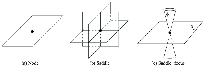
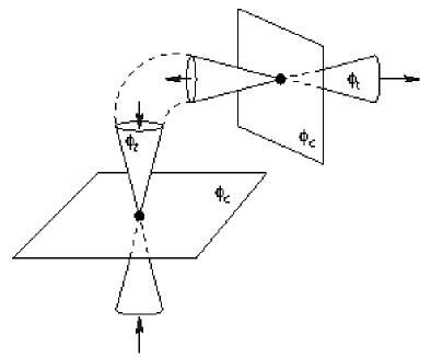
where $\phi_{c}$ is the time independent component and $\phi_{t}$ the time dependent component [17]. Since $\phi_{c}$ does not contain time derivative of $J$ it is associated with the linear component of the vector field and $\phi_{t}$ with the nonlinear component. In the neighborhood of fixed points $\mbox{X}^{*}$, the time independent component of the flow curvature manifold corresponds to the osculating plane [17]. As a consequence, the attractor takes the shape of $\phi_{c}$ in this neighborhood because the osculating plane cannot be crossed by a trajectory. This results from the fact that the osculating plane is invariant with respect to the flow. In all cases, the flow curvature manifold is thus made of a plane parallel to the osculating plane. In the case of a saddle, time-independent component $\phi_{c}$ is also made of two additional transverse planes (Fig. 1b). The fixed point is at the intersection of these three planes. The two complex conjugated eigenvalues of saddle-focus fixed points induce a non null time-dependent component which takes the form of two elliptic paraboloïds, one associated with the each branch of the 1D manifold of the fixed point (Fig. 1c). Fixed points of a saddle-focus type are the only ones with a non-null time-dependent component $\phi_{t}$.

Figure 1: Generic shapes of the flow curvature manifold in the neighborhood of fixed points. There is a time dependent component only for a saddle-focus fixed point.

3 Rössler-like systems

The way according which the flow curvature manifold structures the flow is now illustrated for Rössler-like systems, that is, for systems which have Rössler-like attractors for their solutions.

3.1 Systems with two fixed points

Let us start with the original Rössler system [3]:

$$\left\{\begin{array}[]{l}\dot{x}=-y-z\\ \dot{y}=x+ay\\ \dot{z}=b+z(x-c)\,.\end{array}\right.$$ (9)

We choose to center the Rössler system but this is not compulsory for our analysis. The Rössler system is thus centered through a rigid displacement, that is, the inner fixed point, $F_{-}$, is moved to the origin of the phase space $\mbox{\bbfnt R}^{3}(x,y,z)$. In the translated coordinate system, the equations for the centered system are

$$\left\{\begin{array}[]{l}\dot{x}=-y-z-y_{-}-z_{-}\\ \dot{y}=x+ay+x_{-}+ay_{-}\\ \dot{z}=b+z(x+x_{-}-c)+z_{-}x+z_{-}(x-c)\end{array}\right.$$ (10)

where $\frac{x_{-}}{a}=-y_{-}=z_{-}=\frac{c-\sqrt{c^{2}-4ab}}{2a}$ are the coordinates of the inner fixed point of the Rössler system (9). The system may then be rewritten as:

$$\left\{\begin{array}[]{l}\dot{x}=-y-z\\ \dot{y}=x+ay\\ \dot{z}=\tilde{b}x+z(x-\tilde{c})\,.\end{array}\right.$$ (11)

where $\tilde{b}=z_{-}$ and $\tilde{c}=c-x_{-}$. This centered Rössler system has one fixed point $F_{-}$ located at the origin of the phase space and another one located at

$$F_{+}=\left|\begin{array}[]{l}x_{+}=\tilde{c}-a\tilde{b}\\[5.69046pt] \displaystyle y_{+}=-\frac{x_{+}}{a}\\[5.69046pt] \displaystyle z_{+}=\frac{x_{+}}{a}\end{array}\right.\,.$$ (12)

The structure of the flow near the origin and along the $x$-$y$ plane is governed to a large extent by the unstable fixed point $F_{-}$ (previously designated as the inner fixed point). This causes the flow to “spiral around” this point. On a larger scale, the flow in the Rössler attractor wraps around the one-dimensional unstable manifold associated with the outer fixed point $F_{+}$.

(a) Two branch template		(b) Four branch template

Figure 2: Templates for two different chaotic attractors solution to the Rössler system. Typical parameter values: $b=2$ and $c=4$. Template (a) is obtained with $a=0.432$ and template (b) for $a=0.52$.

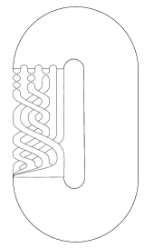
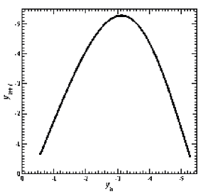
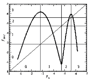
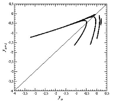
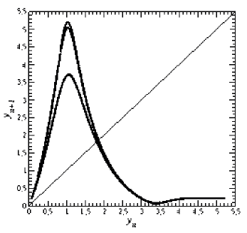
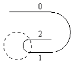
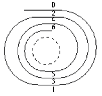
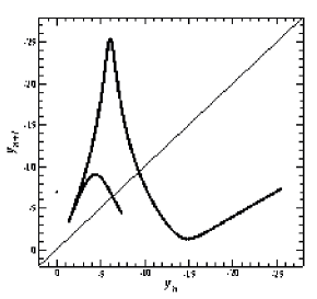
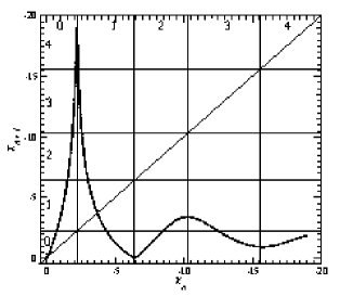
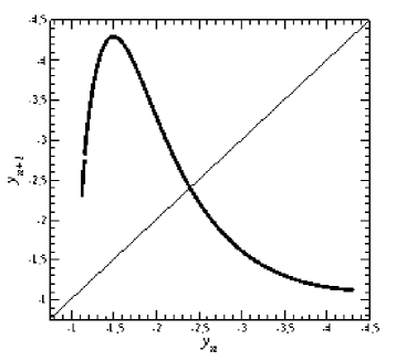
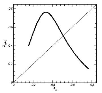
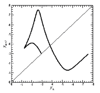
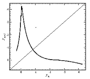
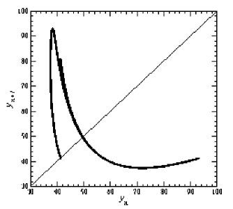
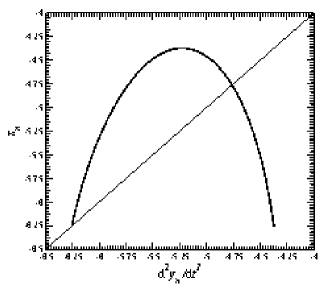
The simplest chaotic attractor solution to the Rössler system has a topology which can be described by a template with two branches as shown in Fig. 2a [20]. Its first-return map to a Poincaré section presents two monotonic branches (Fig. 3a). When parameter $a$ is increased, the attractor after a sequence of bifurcations becomes of funnel type, that is, characterized by a first-return map to a Poincaré section with many monotone branches (four in the case shown in Fig. 3b). The template has therefore two additional branches (Fig. 2b) compared to the previous template (Fig. 2a). In order to describe the way in which monotonic branches are developed and visited, a partition of the attractor can be defined according to the critical points (extrema) of the first-return map (Fig. 3b). A transition matrix is thus defined according to the panels where at least one point can be found. In the case of the first-return map shown in Fig. 3b, all panels are visited and the corresponding transition matrix is

$$\Gamma=\left[\begin{array}[]{cccc}~{}1{}&~{}1{}&~{}1{}&~{}1{}\\ 1&1&1&1\\ 1&1&1&1\\ 1&1&1&1\end{array}\right]\,.$$ (13)

A detailed study of the Rössler attractor can be found in [20].

(a) $a=0.432$		(b) $a=0.52$

Figure 3: First-return map to a Poincaré section of two different chaotic attractors solution to the Rössler system. Typical parameter values: $b=2$ and $c=4$.

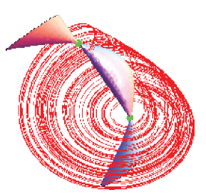
According to the generic shapes for the time-independent component of the flow curvature manifold identified in the previous section, a scheme of the flow curvature manifold can be drawn as shown in Fig. 4. The inner fixed point $F_{-}$ has a plane associated with its unstable 2D manifold and an elliptic paraboloïd centered on its stable 1D manifold. The outer fixed point $F_{+}$ has a elliptic paraboloïd associated with its unstable 1D manifold and a plane corresponding to the stable 2D manifold. In all systems investigated in this paper the inner fixed point has a 2D unstable manifold and those associated with the outer fixed point is 1D. To our knowledge, there is no continuous dynamical system producing an attractor topologically equivalent to the Rössler attractor, and surrounding a fixed point with a 2D stable manifold.

Figure 4: Scheme of the flow curvature manifold for the Rössler attractor. The two elliptic paraboloïds from the fixed points are joined to form a single closed ellipsoïd.

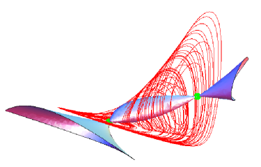
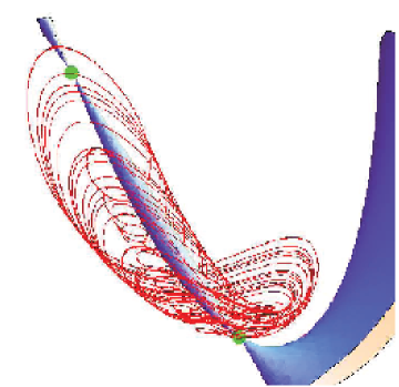
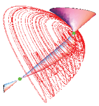
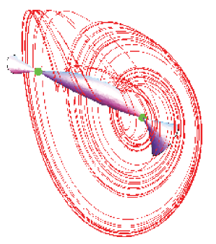
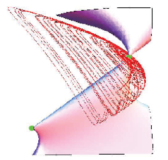
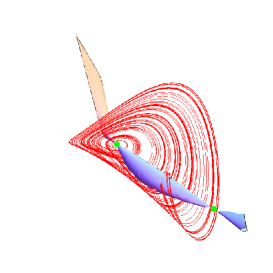
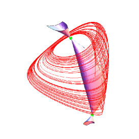
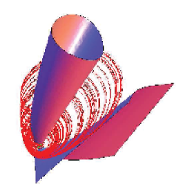
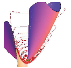
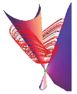
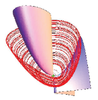
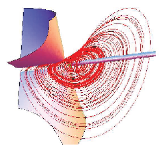
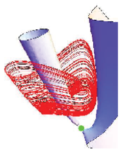
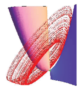
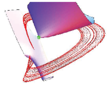
The two components of the flow curvature manifold of the Rössler system are shown in Fig. 5. As expected, in the neighborhood of the inner fixed point, time dependent component of the flow curvature manifold is tangent to the osculating plane, that is, nearly parallel to the $x$-$y$ plane. Component $\phi_{t}$ presents an elliptic paraboloïd at each side of the 2D manifolds of the fixed points. Between the two fixed points, these elliptic paraboloïds are joined to form a closed ellipsoïd (Fig. 5b). The trajectory wraps around a significant part of this closed ellipsoïd. Close to the inner fixed point, the trajectory crosses component $\phi_{t}$. Note that the boundary of the non visited neighborhood of the inner fixed point roughly corresponds to the location where the trajectory crosses component $\phi_{t}$. Such an intersection between the trajectory and component $\phi_{t}$ could be an explaination to the limitation to the development of the dynamics. According to such an assumption, such a crossing could be responsible for the pruning of periodic orbits observed in the neighborhood of the inner fixed point [20]. This is confirmed by the fact that, for $a=0.43295$, the trajectory visits the neighborhood of the inner fixed point and does not intersect component $\phi_{t}$.

(a) Time-independent component $\phi_{c}$	(b) Time-dependent component $\phi_{t}$

Figure 5: The two components of the flow curvature manifold $\phi$ for the Rössler system with parameter values: $a=0.556$, $b=2$ and $c=4$.

Figure 6: Time-dependent component $\phi_{t}$ of the flow curvature manifold for the Rössler system with parameter values: $a=0.43295$, $b=2$ and $c=4$.

Nine other Rössler-like systems were investigated. All the other systems investigated in the subsequent part of this paper can be written under the general form

$$\left\{\begin{array}[]{l}\dot{x}=a_{2}y+a_{3}z+a_{4}xz+a_{5}z^{2}\\[2.84544pt] \dot{y}=b_{1}x+b_{2}y+b_{3}z+b_{4}y^{2}+b_{5}z^{2}\\[2.84544pt] \dot{z}=c_{1}x+c_{2}y+c_{3}z+c_{4}xy+c_{5}xz+c_{6}x^{2}\\[2.84544pt] \end{array}\,.\right.$$ (14)

Only coefficents $a_{i}$, $b_{j}$ and $c_{k}$ are reported in Tab. 1. In all of these systems but one, the elliptic paraboloïds emerging from the fixed points form a closed ellipsoïd (Figs 5b and 7).

Table 1: Specific coefficients of each system here investigated. Compared to their original form as published in [3] and [19], each system was centered, that is, the inner fixed point was located at the origin of the phase space.

		$\dot{x}=$				$\dot{y}=$					$\dot{z}=$
		$y$	$z$	$xz$	$z^{2}$	$x$	$y$	$z$	$y^{2}$	$z^{2}$	$x$	$y$	$z$	$xy$	$xz$	$x^{2}$
System		$a_{2}$	$a_{3}$	$a_{4}$	$a_{5}$	$b_{1}$	$b_{2}$	$b_{3}$	$b_{4}$	$b_{5}$	$c_{1}$	$c_{2}$	$c_{3}$	$c_{4}$	$c_{5}$	$c_{6}$
Rössler		-1	-1	0	0	+1	$+a$	0	0	0	$\tilde{b}$	0	$-\tilde{c}$	0	+1	0
Sprott F		-1	+1	0	0	+1	$+a$	0	0	0	0	0	-1	0	0	+1
Sprott G		-1	+1	0	0	+1	$+a$	0	0	0	0	0	$-b$	+1	0	0
Sprott H		-1	0	0	+1	+1	$+a$	0	0	0	+1	0	$-1$	0	0	0
Sprott K		-1	0	+1	0	+1	$+a$	0	0	0	+1	0	$-b$	0	0	0
Sprott M		-1	0	0	0	$+a$	0	+1	0	0	$+b$	0	-1	0	0	-1
Sprott O		+1	0	0	0	+1	0	-1	0	0	+1	$+a$	0	0	+1	0
Sprott P		$+a$	+1	0	0	-1	0	0	+1	0	+1	+1	0	0	0	0
Sprott Q		-1	0	0	0	$+a$	$+b$	0	0	+1	+1	0	-1	0	0	0
Sprott S		+1	0	0	0	0	$-a$	$-b$	0	0	+2	+1	0	0	0	+1

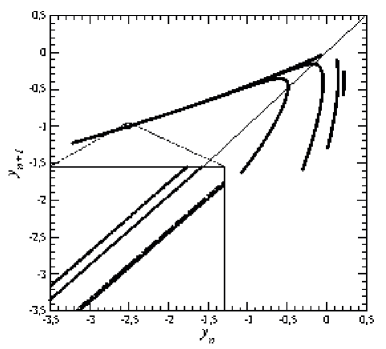
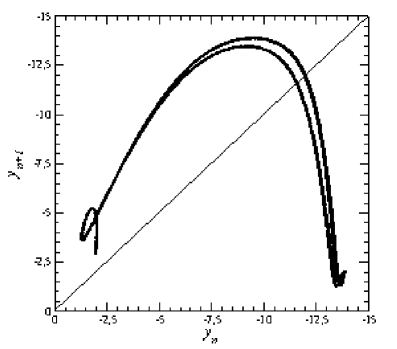
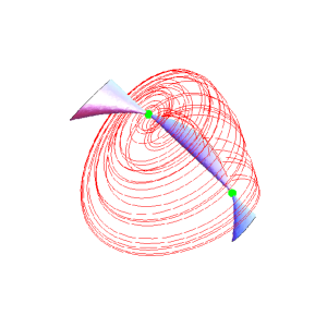
For instance, we observe that Sprott systems F and H produce well developed and similar funnel attractors (Figs. 7a and 7b). For these two systems, the trajectory wraps around component $\phi_{t}$ — and therefore does not cross it — almost everywhere between the two fixed points. First-return map to a Poincaré section of attractors solution to Sprott systems F and H have unusual shapes. Four decreasing monotonous branches are clearly distinguished and a blow up shows four increasing branches (Figs. 7a and 7b). The map has thus eight branches. Such a feature results from the numerical difficulties in computing a proper Poincaré section. Sprott system Q also does not present a trajectory crossing component $\phi_{t}$ too but its funnel structure is less developed (Fig. 7c) than the one of Sprott systems F and H. In particular, the first-return map has only two branches (Fig. 7c). The main departure between these systems could be how fast the trajectory wraps around component $\phi_{t}$.

Chaotic attractor	First-return map
(a) Sprott system F, $a=0.5$
(b) Sprott system H, $a=0.5$
(c) Sprott system Q, $a=3.1$ and $b=0.5$

Figure 7: Chaotic solutions to Sprott system F, H and Q.

In order to roughly quantify this dynamical property, we compute a wrapping number defined as

$$W=\frac{\omega}{\lambda_{3}}D_{F_{+}-F_{-}}$$ (15)

where $\omega$ is the imaginary part of the complex conjugated eigenvalues of the outer fixed point, $\lambda_{3}$ its real eigenvalue and $D_{F_{+}-F_{-}}$ the distance between the two fixed points $F_{+}$ and $F_{-}$. For the three Sprott systems F, H and Q, we obtained $W_{F}=59.4$, $W_{H}=48.5$ and $W_{Q}=0.2$, respectively. Obviously, the trajectory solution to Sprott system Q wraps more slowly than trajectories solution to Sprott systems F and H. The dynamics of Sprott system Q is therefore less developed. In this case, such a limitation results from the eigenvalues of the outer fixed point.

It must be pointed out that the eigenvalues of the outer fixed point do not explain the development of all attractors investigated here. Indeed, when wrapping numbers $W$ are computed for the five other Sprott systems reported in Tab. 1, we got

$$\begin{array}[]{cc}W_{S}=3.8<W_{O}=4.3<W_{P}=8.5<W_{M}=14<...\\[2.84544pt] ...<W_{G}=21.3<W_{K}=27.1\,.\end{array}$$

In particular, $W_{K}$ is significantly greater than $W_{S}$ but the attractor solution to Sprott system S has an attractor (Fig. 9) which is not significantly more developed than the attractor solution to Sprott system K (Fig. 8): the latter presents a unimodal map (Fig. 8b) and the former a three branches map (Fig. 9b) where the third branch is rather small. Moreover, $W_{K}$ is around the half of $W_{F}$ and a more developed dynamics (at least four branches) was expected. The major ingredient, observed in Sprott systems K and S but not in systems F and H, is that the trajectory intersects the time-dependent component $\phi_{t}$. Such an intersection is viewed as being the main reason for the limitation of the dynamics, that is, of the number of monotonous branches in the first-return map.

(a) Chaotic attractor	(b) First-return map

Figure 8: Chaotic behavior solution to Sprott system K. Parameter values: $a=0.35$ and $b=0.5$. Component $\phi_{t}$ is not a closed ellipsoïd due to a singularity which appears when solving $\phi(x,y,z)=0$. By applying the implicit function theorem, we can express $z=\Psi(x,y)$ in terms of $x$ and $y$ where there is a singularity in $x$ inducing numerical artifacts.

The structure of Rössler-like attractors therefore depends on the fixed points (and their eigenvalues) and, the interplay between the flow curvature manifold and the trajectory. The core of the time-dependent component $\phi_{t}$ can be considered as an axis around which the trajectory wraps when there is no intersection between the trajectory and component $\phi_{t}$. The four remaining Sprott systems with two fixed points are quite similar to the case of Sprott system S (Fig. 10).

(a) Chaotic attractor	(b) First-return map

Figure 9: Chaotic behavior solution to Sprott system S. Parameter values: $a=0.99$ and $b=3.8$.

(a) Sprott system G	(b) Sprott system M
$a=0.42$ and $b=1.29$	$a=1.95$ and $b=1.65$
(c) Sprott system O	(d) Sprott system P
$a=2.67$ and $b=0.5$	$a=2.68$

Figure 10: Chaotic attractors solution to Rössler-like systems with their two fixed points (designated by green circles in the figures) and the time-dependent component of their flow curvature manifold. Parameter values correspond to the most developed attractor we identified for each system.

(a) With intersection		(b) Without intersection

Figure 11: Scheme of the transverse structure to the flow observed in a Poincaré section with component $\phi_{t}$ (dashed line). When the trajectory wraps around $\phi_{t}$ the number of branches in the first-return map — or equivalently in the template — is limited by the ratio $W$ (b). Once there is an intersection between the trajectory and component $\phi_{t}$, the number of branches can no longer increase because the trajectory is not longer in the neighborhood of component $\phi_{t}$ (a).

In fact, when the trajectory intersects component $\phi_{t}$, it presents a folding rather than a wrapping structure. Once the trajectory crossed component $\phi_{t}$ and described a fold, it is no longer located in a zone of the phase space where there is a structure (component $\phi_{t}$) around which it can wrap (Fig. 11a). The corresponding attractor can no longer develop new branches and the “funnel” type is quite limited (most often three branches in the first-return map). The probability having an intersection between the trajectory and component $\phi_{t}$ seems to be greater than not. This would explain why limited funnel attractors are more often observed.

3.2 Systems with a single fixed point

In his exhaustive search procedure, Sprott also found systems with a single fixed point. Seven of them will be investigated in this section. Once these systems were centered, they have the general form (14) and their cœfficients are reported in Tab. 2. One system proposed by Thomas [21] and two by Malasoma [15] were also considered. For all of these systems, parameter values used for this study correspond to the most developed chaotic attractor we observed in these systems.

Table 2: Specific coefficients for the systems with a single fixed point here investigated. The last four systems — Sprott systems L and N, and Malasoma systems A and B — produce an inverted Rössler-like chaotic attractor.

		$\dot{x}=$		$\dot{y}=$				$\dot{z}=$
		$y$	$z$	$x$	$y$	$z$	$z^{2}$	$x$	$y$	$z$	$xy$	$y^{2}$
System		$a_{2}$	$a_{3}$	$b_{1}$	$b_{2}$	$b_{3}$	$b_{5}$	$c_{1}$	$c_{2}$	$c_{3}$	$c_{4}$	$c_{7}$
Sprott D		-1	0	+1	0	+1	0	0	+1	$+a$	0	1
Sprott I		$-a$	0	+1	0	+1	0	+1	0	-1	0	+1
Sprott J		$+a$	0	-1	0	+1	0	+1	+1	$-a$	0	0
Sprott R		-1	0	0	0	+1	0	$+a$	$-\frac{b}{a}$	-1	+1	0
Thomas		+1	0	-1	$+a$	-1	0	0	0	$-c$	0	+1
Sprott L		-1	0	$+a$	0	+1	0	0	$+2b$	-1	0	$+b$
Sprott N		$-a$	0	+1	0	$+\frac{2}{a}$	+1	0	+1	$-a$	0	0
Malasoma A		+1	0	0	$-a$	+1	0	-1	0	0	+1	0
Malasoma B		0	+1	0	$-a$	+1	0	-1	0	0	+1	0

(a) Sprott system J, $a=1.76$
(b) Thomas system, $a=0.28$ and $c=2$

Figure 12: Two systems with a single fixed point. The trajectory crosses component $\phi_{t}$ of the flow curvature manifold. This limits the development of the attractor.

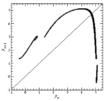
The Sprott system J and Thomas system present a time-dependent component which is crossed by the trajectory (Fig. 12). Their attractors are therefore not so developed as in the previous case. As observed for systems with two fixed points, once the trajectory crosses component $\phi_{t}$ of the flow curvature manifold, it is no longer possible to continue to develop the wrapping process. The resulting attractor is slightly more developed than a unimodal attractor. Sprott system J presents five branches, two of them being under the first two branches (Fig. 12a). In particular, the small increasing branch is quite difficult to distinguish from the first large increasing branch due to the difficulty of computing a well-defined Poincaré section. Thomas system is quite similar to Sprott system J. The advantage of Thomas system is that a safe Poincaré section can be easily computed. As a consequence, its first-return map clearly presents five monotonous branches (Fig. 12b). In both cases, there are two well developed branches and three others that are not very developed. The corresponding transition matrix

$$\Gamma=\left[\begin{array}[]{ccccc}~{}1{}&~{}1{}&~{}1{}&~{}1{}&~{}1{}\\ 1&1&1&1&1\\ 1&1&0&0&0\\ 1&1&0&0&0\\ 1&1&0&0&0\end{array}\right]$$ (16)

reveals that, for instance, points in branches labelled 2, 3 and 4 are necessarily followed by points located in the first two branches (labelled 0 and 1, respectively). According to our views, this feature results from intersections between the trajectory and component $\phi_{t}$.

Sprott systems D and I present a different configuration. The trajectory does not intersect component $\phi_{t}$ around which it wraps. In the case of Sprott system D (Fig. 13a), there are numerical artifacts in computing component $\phi_{t}$ due to a singularity occuring when solving $\phi(x,y,z)=0$. As a consequence, a spurious part is obtained in addition to the two elliptic paraboloïds usually found. The trajectory intersects the spurious part of component $\phi_{t}$ and we can consider that there is no intersection between the trajectory and component $\phi_{t}$. What limits the dynamics is in fact the two pure imaginary eigenvalues of the fixed point which forbid the trajectory visiting the neighborhood of the fixed point. A similar conclusion is obtained for Sprott system I (Fig. 13b) where the fixed point has two complex conjugated eigenvalues with very small real parts. In both cases, the development of the attractors can be understood using fixed point eigenvalues combination with component $\phi_{t}$.

(a) Sprott system D, $a=2.3$
(b) Sprott system I, $a=0.25$

Figure 13: Two systems with a single fixed point producing a quite limited chaotic attractor. System D has two pure imaginary eigenvalues and system I has two complex conjugated eigenvalues with small real parts (Re$(\lambda_{\pm})\approx 0.07$).

First-return maps to a Poincaré section of these two attractors present two monotonic branches that are not fully developed. These two chaotic regimes are therefore less developed than previous cases that have three monotonic branches in their first-return maps.

(a) Chaotic attractor	(b) First-return map

Figure 14: Sprott system R with a single fixed point. The trajectory wraps around component $\phi_{t}$. One of the elliptic paraboloïds emerging from the fixed point results from a singularity occuring when solving $\phi(x,y,z)=0$ as for Sprott system K. This leads to a funnel chaotic attractor. Parameter values: $a=0.90$ and $b=0.395$.

3.3 Inverted Rössler-like chaos

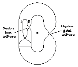
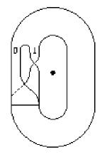
Among Sprott systems with a single fixed point, two of them, namely systems L and N, produce chaotic attractors which have an inverted Rössler-like topology. Typically, an inverted Rössler-like attractor — also named inverted Horseshoe attractor [7] — differs from a “direct” Rössler-like attractor by a global torsion of a half-turn. The usual organization with the order preserving branch close to the inner fixed point and the order reversing branch at the periphery of the attractor (Fig. 2a) is therefore inverted and the order reversing branch of the first-return map is close to the inner fixed point and the order-preserving branch is at the periphery of the attractor (Fig. 15b).

(a) Template with global torsion		(b) Equivalent template

Figure 15: A template with a negative global half-turn and a positive local half-turn (a) can be reduced under an isotopy to an inverted Rössler-like template (b), that is, without any global half-turn and with a single local half-turn (here negative). The branch with a local half-turn of the reduced template is associated with the decreasing branch of the first-return map and is located near the inner fixed point (designated by $\bullet$).

Sprott systems L and N do not present a component $\phi_{t}$ very different from those obtained for systems I and J, for instance. Nevertheless, the two attractors (Figs. 16a and 16b) are located relatively far from the fixed point (compared to previous cases). In these two cases, the influence of component $\phi_{t}$ seems to be induced by the second elliptic paraboloïd which constrains the attractor by its periphery. Funnel attractors would not be observed due to this external constraint.

(a) Sprott system L, $a=3.87$ and $b=0.91$
(b) Sprott system N, $a=4.2$

Figure 16: Chaotic attractors solution to Sprott systems L and N. In both cases, the trajectory spirals arouund component $\phi_{t}$ of the flow curvature manifold.

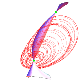
Two other systems with a single fixed point were proposed by Malasoma [15]. They are minimal in the sense that it is not possible to obtain chaotic system with a simpler algebraic structure. From the flow curvature manifold point of view, these two systems are similar and only one of them is discussed here. As for many minimal systems, the chaotic domain in the parameter space is quite limited. The attraction basin is also quite small. Component $\phi_{t}$ presents an unusual shape with a cylindrical aspect for one of the two elliptic paraboloïds (Fig. 17). Once again, this results from numerical artefacts induced by a singularity appearing when solving $\phi(x,y,z)=0$. In this case, the trajectory solution to Malasoma system A intersects component $\phi_{t}$. Compared to all cases previously discussed, this is the first example for which the whole attractor intersects component $\phi_{t}$ in the non ambiguous part. According to our assumption, such a global intersection strongly limits the development of the chaotic attractor. But the limitation of the dynamics occurs in a slighly different way than the previous two cases. The first-return map presents a fully developed unimodal map (Fig. 17b), that is, more developed than those computed for Sprott systems D and I (Figs. 13). Nevertheless, real parts of the complex conjugated eigenvalues of Malasoma system A is clearly non zero. The intersection of the whole attractor with component $\phi_{t}$ limits the region of the phase space where the attractor can exist. In particular, it constrains the attractor to be developed quite far from the fixed point. As a consequence, the branch without any half-turn is not observed and this is an inverted Rössler-like chaos.

(a) Chaotic attractor	(b) First-return map

Figure 17: Chaotic attractor solution to Malasoma system A. Component $\phi_{t}$ presents an unusual shape and crosses all the attractor, thus limiting the chaotic regime. Parameter value: $a=2.017$. Initial conditions: $x_{0}=0.1$, $y_{0}=1$ and $z_{0}=1.9$.

Among these seven systems with a single fixed point, one — Sprott system R — presents a time-dependent component $\phi_{t}$ around which the trajectory wraps (Fig. 14). Nevertheless, its time-dependent component is affected by a singularity which prevents us from avoiding a spurious third elliptic paraboloïd. It is therefore difficult to make conclusions about this system. The presence of a second fixed point is therefore not required to observe a chaotic attractor of a funnel type. The relevant ingredient is indeed that the trajectory wraps around component $\phi_{t}$ without any intersection with it.

4 Conclusion

It is still a very challenging problem to connect topological properties of phase portraits with some analytical properties of the governing equations. Fixed points are certainly the first step for such a connection. But the whole topological structure cannot be obtained from them. In this paper, we showed that the flow curvature manifold can bring some additional light on what structures the phase portrait. This manifold was split into one time-dependent and one time-independent components. We showed that the time-independent component was tangent to the osculating plane in the neighborhood of the inner fixed point. Our results suggest that the time-dependent component is mainly responsible for limiting the development of chaotic attractors when they are crossed by the trajectory. An attractor is thus not only constrained by fixed points and some other solutions — unstable periodic orbits for instance — co-existing in the phase space, but by the flow curvature manifold too. The next step is now to investigate permeability properties of the flow curvature manifold to better understand why the time dependent component $\phi_{t}$ of the flow curvature is not always crossed by trajectories.

Acknowledgements

C. Letellier thanks L. A. Aguirre, R. Gilmore, U. Freitas and J.-M. Malasoma for stimulating discussions. Both of us thank Aziz-Alaoui for stimulating remarks while he was preparating his own slides at the International Workshop-School Chaos and Dynamics in Biological Networks in Cargèse (Corsica).

References

- [1] D. Ruelle & F. Takens, On the Nature of Turbulence, Communications in Mathematical Physics, 20, 167-192, 1971.
- [2] J. P. Gollub & H. L. Swinney, Onset of turbulence in a rotating fluid, Physical Review Letters, 35, 927-930, 1975.
- [3] O. E. Rössler, Chaotic behavior in simple reaction systems, Zeitschrift für Naturforschung A, 31, 259-264, 1976.
- [4] H. Haken, Analogy between higher instabilities in fluids and lasers, Physics Letters A, 53 (1), 77-78, 1975.
- [5] J. P. Eckmann & D. Ruelle, Ergodic theory of chaos and strange attractors, Review of Modern Physics, 57, 617-656, 1985.
- [6] H. D. I. Abarbanel, R. Brown, J. J. Sidorowich & L. Sh. Tsimring. The analysis of observed chaotic data in physical systems, Review of Modern Physics, 65 (4), 1331-1388, 1993.
- [7] R. Gilmore & M. Lefranc, The topology of chaos, Wiley, 2002.
- [8] T. D. Tsankov & R. Gilmore, Strange attractors are classified by bounding tori, Physical Review Letters, 91 (13), 134104, 2003.
- [9] C. Letellier, E. Roulin & O. E. Rössler, Inequivalent topologies of chaos in simple equations, Chaos, Solitons & Fractals, 28, 337-360, 2006.
- [10] H. Poincaré, Sur le Problème des trois corps et les équations de la dynamique, Acta Mathematica, 13, 1-279, 1890.
- [11] I. Bendixson, Sur les Courbes définies par des équations différentielles, Acta Mathematica, 24, 1-88, 1901.
- [12] Z. Fu & J. Heidel, Non-chaotic behavior in three-dimensional quadratic systems, Nonlinearity, 10, 1289-1303, 1997.
- [13] J. C. Sprott & S. J. Linz , Algebraically simple chaotic flows, Internation Journal in Chaos Theory and Applications, 5, 3-22, 2000.
- [14] J. C. Sprott, Simplest dissipative chaotic flows, Physics Letters A, 228, 271-274, 1997.
- [15] J.-M. Malasoma, A new class of minimal chaotic flows, Physics Letters A, 305, 52-58, 2002.
- [16] J.-M. Ginoux, Differential geometry applied to dynamical systems, World Scientific Nonlinear Science, Series A, Vol. 66, 2009.
- [17] J.-M. Ginoux, B. Rossetto & L. O Chua, Slow invariant manifolds as curvature of the flow of dynamical systems, International Journal of Bifurcations & Chaos, 18 (11), 3409-3430, 2008.
- [18] G. Darboux, Sur les équations différetielles algébriques du premier ordre et du premier degré, Bulletin des Sciences Mathématiques, Série 2, 2, 60-96, 123-143, 151-200, 1878.
- [19] J. C. Sprott, Some simple chaotic flows, Physical Review E, 50 (2), 647-650, 1994.
- [20] C. Letellier, P. Dutertre & B. Maheu, Unstable periodic orbits and templates of the Rössler system: toward a systematic topological characterization, Chaos, 5 (1), 271-282, 1995.
- [21] R. Thomas, Nullclines and nullclines intersection, International Journal of Bifurcation and Chaos, 16 (10), 3023-3033, 2006.