Reconstruct the Distance Duality Relation by Gaussian Process
Yi Zhang a,111Email: zhangyia@cqupt.edu.cn
aCollege of Mathematics and Physics, Chongqing University
of Posts and Telecommunications,
Chongqing 400065, China
Abstract
In this letter, the distance-duality (DD) relation is reconstructed by Gaussian process (GP) which is cosmological model-independent. Generally, the GP plays two important roles. One is to shape the tendency which denotes the deviation from the DD relation, the other one is to produce the luminosity-distance (LD, ) and the angular-diameter-distance (ADD, ) data at the same redshift. The shapes of are given out based on SNe Ia (Type Ia supernovae) data with different light-curve fitters (including MLCS2K2 and SALT2) and ADD data with different galaxy cluster morphologies (including the elliptical and spherical models). The data related to MLCS2K2 light-curve fitter have higher values of compared to that related to the SALT2 light-curve fitter. As for the morphology of galaxy cluster, the DD relation is favored by the elliptical one.
1 Introduction
In astronomy, the distance-duality (DD) relation is of fundamental importance as it connects the luminosity-distance (LD, ) and the angular-diameter-distance (ADD, ). Initially, the DD relation () is called Etherington relation [2, 3]. It is valid in any cosmological background where photons travel along null geodesics and where photon number is conserved. In fact, many geometric properties are invariant when the roles of source and observer in astronomical observations are transposed. As the key element of analyzing the galaxies observations, the Cosmic Black-body Radiation (CBR) observations and the gravitational lensing, DD relation has been usually used in cosmology for granted. A major crisis would arise for observational cosmology if DD relation was found to not be true. However, if there were deviations from a metric theory of gravity or variations of fundamental constants, or photons not traveling along unique null geodesics, the DD relation would be violated theoretically [5].
In the earlier work [6, 7, 8, 9, 10, 11, 12, 13, 14, 15, 16, 17, 18], a new parameter
| (1) |
is defined to denote the departure from DD relation. was tested as constant and parameterizations [19, 20, 21, 22, 23, 24, 25]. Maximum likelihood estimation is employed to determine the most probable values which needs sample first. One way of getting sample is to combine the distance results from both observation and theoretical expressions. Obviously, the test depends on cosmological model heavily. The LD or ADD data could be fixed by the CDM model with the fixed observational cosmological parameters. Observationally, the LD data could be derived from Type Ia supernovae (SNe Ia) compilation; while the ADD data could be estimated from astrophysical sources such as Baryon acoustic oscillation (BAO) data, galaxy clusters, FRIIb galaxies,radio galaxies, etc.. However, the main problem for the observational-only data is that the observational LD and ADD data are not at the same redshift. Therefore, the observational data must be combined with the theoretical one. Anyway, an interesting contradiction appeared: Refs.[10, 17, 18, 16] saw no evidence of violation for DD relation while a violation of the DD relation is concluded by Ref.[7].
In recent work, local regression methods are used (e.g. Ref.[14]) to avoid introducing errors due to the redshift mismatch. Specially, the method of binning LD data with the redshift range worth attentions. In Refs.[22, 23, 25], the DD relation is found to discriminate the morphology of cluster galaxy. For example, Li et al. [22] found that the DD relation can be accommodated at confidence level (CL) for the elliptical one, and at CL for the spherical one.
Though the data sample based on the criterion is model-independent, the derived is still model-dependent. In principle, the DD relation should be tested only from the astronomical observations, i.e. finding cosmological sources whose intrinsic luminosity and intrinsic sizes are known. Gaussian process (GP) is a powerful non-linear interpolation tool which allows one to reconstruct a function from data without assuming a parameterization [26, 27, 28, 29]. It has been applied to cosmology for the equation of state of dark energy [30, 31, 32, 33, 34, 35, 36, 37]. In this letter, the Gaussian process will be applied to reconstruct the DD relation which will play two main roles: to get the shape of and to match the redshifts of the LD and ADD data. SNe Ia data from different light-curve fitters will be investigated. Specificlly, we will use the SNe Ia compilations in Ref.[38, 39] which were derived from both SALT2 and MLCS2K2 light-curve fitters by Kessler et al. and the Union2.1 compilation based on the SALT2 fitter [40]. Furthermore, the ADD sample with different morphological models are chosen as well. The elliptical [41, 42, 43] and the spherical galaxy clusters [44] are used to test the intrinsic shape of cluster.
The letter is organized as follows. In Sec.2, the GP will be introduced. In Sec.3, we will give out the luminosity-distance and the angular-diameter-distance. In Sec.4, the GP is used to get the LD and ADD data at the same redshift. In Sec.5, we will use new samples to test the DD relation, one is based the improved criterion that the redshift difference of ADD and LD should be less than . The other one is based on GP data of the LD and the observational ADD data (or GP data of the ADD and the observational LD data, or both GP data of the LD and ADD). The deviation from will be investigated. And a summary will be given out in Sec.6.
2 Gaussian Process
As a powerful non-linear interpolating tool, Gaussian process is useful for cosmology and astronomy [26, 27, 28, 29]. The GP has been introduced as non-parametric technique and has successfully reconstructed the equation of state of dark energy [30, 31, 32, 33, 34]. Here, the public available code GAPP (Gaussian Processes in Python) [30, 31] is used to reconstruct the DD relation. In the following, if GP was applied, the label “(GP)” would be put after the name of the data.
A Gaussian distribution is a distribution over random variables, while a GP is distribution over functions which has elements of an infinite dimensional space. Here, we give the basic conception of GP which could perform a reconstruction of function from data without assuming function parameterization. In the reconstruction of DD relation, the observational data and the reconstructed data are combined to form a joint distribution. Based on the joint distribution, the GP is given by a mean function with Gaussian error bands, where the function values at different points are connected through a covariance function.
The freedom in GP comes from the chosen covariance function which determines how smooth the process is and how nearby points are correlated. Throughout the whole letter, we will use the Matern covariance function
| (2) |
where are represent two different points, hyper-parameter is the typical change of variable, hyper-parameter is the typical length scale of function, is the Gamma function and is a modified Bessel function with and . The hyper-parameters and could be trained by maximizing the marginal likelihood which only depends on the locations of the observations. Indeed, the GP approach is rather robust to the covariance function choice [26, 27, 28, 29].
3 Observational Data
The deviation from corresponds to the violation of DD relation. Even a small deviation indicates breakdown of fundamental physical theories. It is obvious that the observational ADD and LD data are needed if we want to reconstruct DD relation. In isotropic and homogenous cosmological background, the angular-diameter-distance and luminosity-distance,
| (3) |
are also called standard rulers and standard distances where is the Hubble parameter.
3.1 The Angular-Diameter-Distance Data
Two galaxy cluster data sets which provide the ADD data based on different morphology and dynamics are used here.
The first samples are formed by 25 galaxy clusters in redshift range of [41, 42, 43]. In Ref. [41], cosmological angular-diameter-distance is known from the redshift and the prior knowledge of the cosmology. Based on Eq.(10) in Ref.[41] and assuming the isothermal triaxial cluster profile, the experimental quantity of ADD was calculated which combined X-ray surface brightness and SZE analysis. We call it the ES sample instead of the name in Ref.[41]. And, Ref.[41] also listed the experimental estimate of SS which was assumed with spherical symmetry and reported by Refs. [42, 43]. The data will be used as standard rulers. The ES will be used for morphology comparison. The SS data will be used for data comparisons.
The second samples are defined by the 38 ADD galaxy clusters from Ref.[44] where the cluster plasma and dark matter distributions were analyzed by assuming generalized spherical model. We call it the Spherical Sample (SS). They are in the redshift range of . As reported by Ref.[44], almost all the ADD data are followed by asymmetric uncertainties. To deal with the asymmetric uncertainties, we choose three data dealing methods for comparison and call them SS\@slowromancapi@ , SS\@slowromancapii@ and SS\@slowromancapiii@. The first one addressed this issue by combining the statistical and systematic uncertainties in quadrature [13, 22]:
| (4) |
where the denotes the expected value, is the standard deviation, and are the upper and lower limits of error. We also use the reported value as expected value and the larger flank of each two-sided error as standard deviation [23]
| (5) |
As stressed by Ref.[44], the modeling uncertaintis of the angular diameter distances presented contribute to statistical uncertainties. Therefore, it is reasonable to make the following correction and estimations [45] ,
| (6) |
Specially, the error of and SS data are asymmetrical too. For simplity, they will be dealt by the third method.
3.2 The Luminosity-distance Data
In order to check consistency of GP, we will perform same analysis among SNe Ia samples which have different light-curve fitters. We consider the MLCS2K2 (the current version of Multicolor light-curve Shape method) and SALT2 (the current version of Spectral Adaptive light-curve Template) light curve fitters which are the commonly used. The two different light-curve fitters reflect different assumptions about the nature of color variations in SNe Ia, different approach to training the models using pre-existing data, and different ways of determining parameters.
The SNe Ia data provide the luminosity-distance relation
| (7) |
where is the distance moduli. Anyway, the SALT2 fitter which is a spectral-template-based fit method [40] depends on the cosmological parameter where the cosmological parameters and light-curve parameters are fitted simultaneously. In contrast, there is no such cosmological parameter dependence for the MLCS2K2 fitter [38, 39].
In Ref.[38], the SN Ia data is analyzed with both MLCS2K2 and SALT2 light-curve fitters. It has 288 data set of distance moduli in the redshift range of with a 247 data set in the redshift range of . They are dubbed as MLCS2K2:09 and SALT2:09. The Union2.1 SNe Ia compilation [35] has been analyzed with the SALT2 light-curve fitter and has 580 dataset of in the redshift range of with a 508 dataset in the redshift range of . In principle, the data related to Union2.1 and that related to SALT2:09 should give out similar results.
3.3 Our GP
We give out the details of how we use data with GP. Besides the luminosity-distance and the angular-diameter-distance, the value of is required for getting . As the above section mentioned, the data set of Union2.1 (or MLCS2K2:09) is larger than that of galaxy cluster. To be precise, we use the redshift in the luminosity-distance data to obtain . Technically, we transfer the SNe Ia distance moduli to a new variable .
And, we choose the range of reconstructed redshift as which will cover the our smallest redshift region . And as the observational redshift is in the precision of , the redshift number of GP is chosen as 800. Thus, every observational data in will correspond to a reconstructed one.
At last, as Ref.[30] suggested, we have run Gaussian process repeatedly with different initial conditions for the hyper-parameters (, ) to get a smooth result in case that the optimization of the hyper-parameters getting stuck in a local maximum.
4 Rough Checking of GP
4.1 The GP of LD and ADD
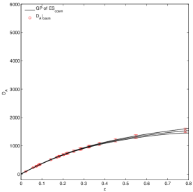
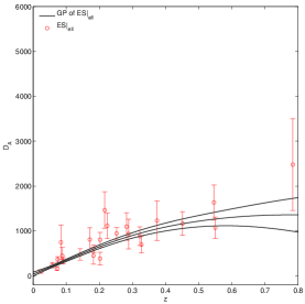
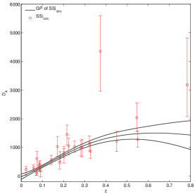
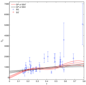
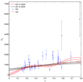
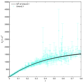
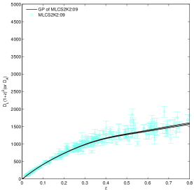
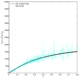
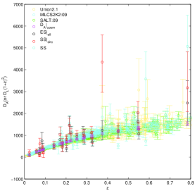
In Figure 1, we present the GP results of the ADD and LD data which show the systematical error of GP result become smaller compared to the original data, especially in the dense data regime. When two observational data are very close, the GP results favor the one with smaller error. Thus, the GP results avoid large deviated data .
Generally, the data from Ref.[41] (, ES and SS) have the same monotone increasing reconstructed shapes. As high redshift data from Ref.[41] is rare, it is reasonable that the error of GP results become large as z increase. The error of GP result is SSES. Specially, the GP result of shape of SS does not favor the (A370) and (MS 1137.5+6625) data.
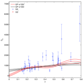
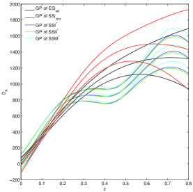
However, the GP results of SS data (SS\@slowromancapi@, SS\@slowromancapii@ and SS\@slowromancapiii@) suffer from systematics of heterogeneous data. The GP results seem consistent with the observational data. But there is no explanation for the high value around . Because based on Eq.3, the value of ADD data should be 0 when . This phenomenon is caused by the lack of SS data in the low redshift. To fix this problem, we use a faked data at with which is close to the value derived from the definition of standard ruler. And its errors , are from the lowest redshift data in the SS sample where . We call the SS with fake data as SS\@slowromancapi@∗, SS\@slowromancapii@∗ and SS\@slowromancapiii@∗. Anyway, the GP results of SS\@slowromancapi@∗, SS\@slowromancapii@∗ and SS\@slowromancapiii@∗ are oscillating.
4.2 The Comparisons
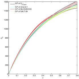
In the left panel of Figure 2, the region of the Union2.1, MLCS2K2:09 and SALT:09 are shown. Roughly, the GP value of is MLCS2K2:09 Union2.1 SALT:09. The GP result of nearly cover all the GP of SNe which indicates the and LD data are consistent.
As the middel panel of Figure 2 shown, the GP tendencies of ES and SS data are nearly the same in the low redshifts where the data are concentrated. And because of the different galaxy morphology, the ES data give out smaller GP result at high redshift. It is expected that the SS data (SS\@slowromancapi@, SS\@slowromancapii@ and SS\@slowromancapiii@) should have the same GP tendency with the SS data because both of them are assumed spherical symmetry. Anyway, the SS obtain a oscillating behavior while the SS data obtain a monotone increasing function. Because of different error dealing methods, the GP result show SS \@slowromancapiii@ (GP) SS \@slowromancapi@ (GP) SS \@slowromancapii@ (GP) with slight differences. The GP of SS \@slowromancapiii@ seems closest to the LD data. The oscillating behavior may be caused by GP but it does not affect the GP of as we will see.
5 Reconstruction of DD relation
5.1 with One GP

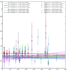
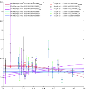
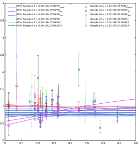
| Union2.1/SS \@slowromancapi@ | MLCS2K2:09/SS \@slowromancapi@ | SALT2:09/SS \@slowromancapi@ | |||
|---|---|---|---|---|---|
| Union2.1/SS \@slowromancapii@ | MLCS2K2:09/SS \@slowromancapii@ | SALT2:09/SS \@slowromancapii@ | |||
| Union2.1/SS \@slowromancapiii@ | MLCS2K2:09/SS \@slowromancapiii@ | SALT2:09/SS \@slowromancapiii@ | |||
| Union2.1/ | MLCS2K2:09/ | SALT2:09/ | |||
| Union2.1/ES | MLCS2K2:09/ES | SALT2:09/ES | |||
| Union2.1/SS | MLCS2K2:09/SS | SALT2:09/SS | |||
| Union2.1/(GP) | MLCS2K2:09/(GP) | SALT2:09/ (GP) | |||
| Union2.1/ES(GP) | MLCS2K2:09/ES(GP) | SALT2:09/ES (GP) | |||
| Union2.1/SS(GP) | MLCS2K2:09/SS(GP) | SALT2:09/SS (GP) | |||
| Union2.1(GP)/ | MLCS2K2:09(GP)/ | SALT2:09(GP)/ | |||
| Union2.1(GP)/ES | MLCS2K2:09(GP)/ES | SALT2:09(GP)/ES | |||
| Union2.1(GP)/SS | MLCS2K2:09(GP)/SS | SALT2:09(GP)/SS |
The model-independent criterion that the redshift difference of the ADD and LD data should be less than was used. In order to avoid the appearance of too many data for one redshift, the criterion is improved to in this letter. Thus we have the so-called sample by combining all the uncertainties in quadrature. The derived values of are more centered around the line compared to Refs.[22, 25]. The redshift range of the SS related sample is , while that of the ES related sample is . The exact number of sample at each ADD redshift are summarized in Table 2. In principle, the GP could be applied to see the tendency of instead of assuming a parameterization of .
5.1.1 Overlap Sample
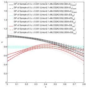
In Figure 3, the Union2.1 and MLCS2K2:09 (or SALT2:09) data are combined as LD data. Meanwhile, the SS (SS\@slowromancapi@, SS\@slowromancapii@ or SS\@slowromancapiii@) data from Ref.[44] and the samples from Ref.[41] (, or ES, or SS) are combined as ADD data. The value of the Union2.1+ MLCS2K2:09/ADD sample seems smaller than that of the Union2.1+SALT2:09/ADD sample. Though the SS\@slowromancapi@, SS\@slowromancapii@, SS\@slowromancapiii@ related data are varied with the error dealing methods, the error dealing methods just affect their reconstruction of on the value slightly. And, only the ES related data give out constant results which is around and not consistent with the DD relation. The samples which are related to spherical symmetry (SS+SS) shape like bulge. The related data are supposed to have a constant reconstruction. But it seems to be affected by the galaxy cluster sample of spherical symmetry which makes a declining trend of . Based on the above discussions, we do not regard the combination of the SS and the ES models a good idea.
5.1.2 Separated Samples
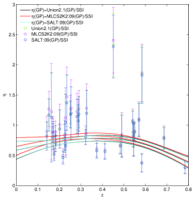
In this section, we will discuss the sample derived from the separated LD and ADD data. The number of every separated sample is enough to have an effective GP as Figure 4 shows. As for the spherical sysmmetry of cluster, the SS related data give out a monotone increasing function. However, all the other samples give out a nearly constant . The MLCS2K2:09/ES data has which is closest to . And, there is no physical explanation for the difference between the SS\@slowromancapi@ ( or SS\@slowromancapii@ or SS\@slowromancapiii@) and SS related data. Respect to the reconstructing results of Union2.1/ and SALT2:09/ in Figure 4 and Table 1, the DD relation() is faved. Meanwhile, the MLCS2K2:09/ result gives out a decreasing tendency and gets with a departure from the DD relation. The difference between the MLCS2K2 and SALT2 fitter will appear in the following.
5.2 GP with Two GPs
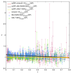
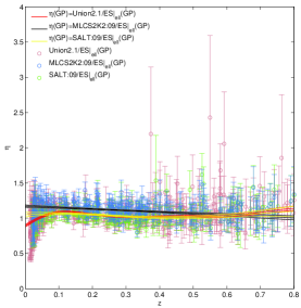
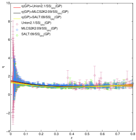
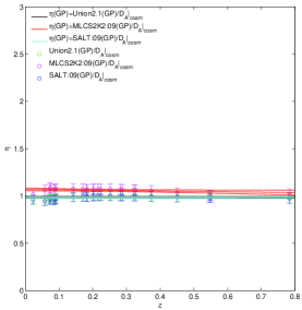
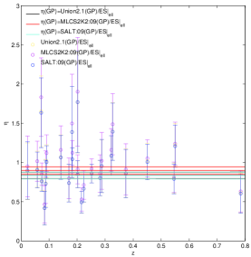
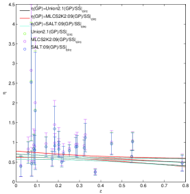
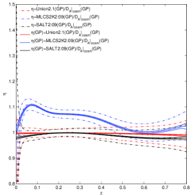
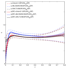
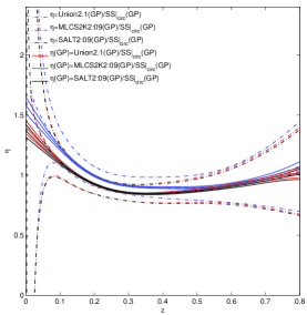

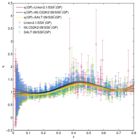
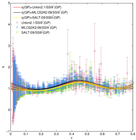
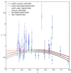
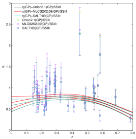
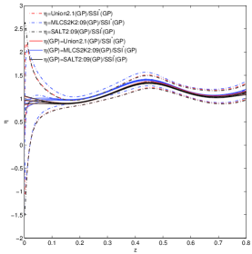
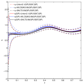
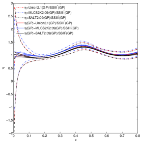
As we have derived the LD and ADD at same redshift by GP in Sec.4, new samples could be constructed from the GP of LD and the observational data of ADD, or from the GP of ADD and the observational data of LD, or from both GP of ADD and LD data. Then, the shape of could be given out by using GP again. We present the new samples in Figure 5 and 6.
Generally speaking, the GP results of shown in Figure 5 and 6 are not reliable. Because they are far from DD relation at low redshift which could be tested by Milky Way observation. This phenomenon may be caused by the lack of observational data at low redshift. We do not analyze the results in the following. And, most of the MLCS2K2:09 related samples have declining trends and larger values than the Union2.1 and SALT2:09 related ones.
The left panels of Figure 5 present the GP result of the LD(or GP)/(or GP) sample. As expected, the Union2.1/(GP) and SALT2:09/(GP) (or Union2.1(GP)/ and SALT2:09(GP)/) samples give out flat trends and suggest no violation of the DD relation. The exact values of are shown in Table 1. These results are not a surprise because the Union2.1, SALT2:09 and data are based on cosmological parameter. Meantimes, It suggests the GP method is effective.
The middle panels in the vertical direction of Figure 5 show the GP results of the LD(or GP)/ES(or GP) sample. Except the MLCS2K2:09/(GP) data, the derived from GP which is related to the ES is flat. The Union2.1(GP)/ES and SALT2:09(GP)/ES suggest that no violation of the DD relation. And, the GP of Union2.1/ES(GP) and SALT2:09/ES(GP) data obtain a constant but below . Especially, the GP of MLCS2K2:09/(GP) has a flat trend as well. The exact value of could be referred to Table 1 as well. It seems the is flat and smaller than the DD relation If ES data play main role.
The right panels of Figure 5 show the GP results of the LD(or GP)/SS(GP) which are declining. The of LD(or GP)/SS(GP) are listed in Table 2 as all which is around . Basically, the SS should have the similar result with the SS samples (SS\@slowromancapi@, SS\@slowromancapii@, SS\@slowromancapiii@) from Ref.[44]. But the SS samples have the bulge effect around which are shown in Figure 6. The three different SS data with different error dealing method do not show obvious difference. And, the bulge effect is hard to explained by physics. It is possible that the bulge behaviors are caused by the GP of the SS sample which favors the data with smaller error bar.
5.3 Discussions
During all the GP reconstructions, no parameterization is assumed. The approach is fully model-independent, only the statistical quantities and covariance matrices are considered in the GP approach.
Here, we concentrate on the test of light-curve fitter. Nearly in all the comparison between MLCS2K2 and SALT2 fitters, the value from the MLCS2K2 fitter is larger than that from SALT2. In Kessler’s work, the constraining result of Equation of State based on CDM model for MLCS2K2:09 is larger than that based on SALT2:09 which indicates MLCS2K2:09 data itself have a higher . From this point of view, our results for DD relation are consistent with Ref.[38].
The connection between the validity of the DD relation and the morphology of galaxy cluster is investigated as well. In Refs.[20, 21], the verification of the DD relation seems to favor an elliptical shape, but for spherical model the validity of the DD relation seems only marginally compatible.
Uzan et.al concluded there is no significant violation of the DD relation for a CDM model by using ADD from X-ray surface brightness and Sunyaev-Zel’dovich effect measurements of galaxy cluster [6]. Our ES sample includes the ADD data used by Ref.[6]. In all the GP related to the ES data, the reconstructions of are nearly constant. This phenomenon suggests the ES favor the DD relation though the value are affected by LD data. In another saying, if the DD relation was correct, it would favor the galaxy morphology of elliptical one.
There is disagreement between our result and the result in Ref.[10] where De Bernardis et al. gave out no violating result of DD relation and found at CL based on the SS. Though GP has improved the error range of SS, the SS\@slowromancapi@, SS\@slowromancapii@ and SS\@slowromancapiii@ related data display bulge behaviors with values smaller than . The GP results of are not affected by the fake SS data at because the sample and the LD(GP)/ADD sample also give out the bulge shapes. Our results based on the SS do not favor the DD relation. When the spherical sample changed to SS, Figure 4 shows increases with redshift, while Figure 5 show decreases with redshift. The incompatible results are not reliable which may be caused by the large error. The spherical samples do not favor the DD relation.
6 The Summary
Based on Gaussian process, we have introduced new reconstructing approachs for DD relation. The DD relation relates the luminosity-distance with the angular-diameter-distance, and it has been widely used in cosmological models. Checking the validity of DD relation with high accuracy may provide probe of exotic physics. GP is a non-parametric technique which could smooth the noise of data. In this letter, it has two effects in our reconstructions: to reconstruct the shape of and to get the LD and ADD data at the same redshift.
The related data of MLCS2K2 light-curve fitter show high values and declining trends in most cases. In contrast, the related data of SALT2 light-curve fitters (Union2.1 and SALT2:09) are easier to get constant . The GPs derived from the Union2.1 and (the standard ruler) data show is close to which suggest GP is an effective method. The reconstructed results related to data show constant in most cases as well. And, for the SS related data, our three different methods of dealing asymmetric errors do not make obvious differences where all the related GP results have bulge shapes. And the varied behavior of the SS related data suggests its large error could not lead to reliable results. Respect to galaxy cluster morphology, the DD relation is favored by the elliptical one.
| The SS | The ES | ||||||
|---|---|---|---|---|---|---|---|
| Name | z | N(Union2.1/SS) | N(SALT:09/SS) | Name | z | N(Union2.1/ES) | N(SALT:09/ES) |
| CL J1226.9+3332 | 0.890 | - | - | MS 1137.5+6625 | 0.784 | - | - |
| MS 1054.5-0321 | 0.826 | - | - | MS 0451.6-0305 | 0.550 | 2 | 1 |
| RX J1716.4+6708 | 0.813 | - | - | CL 0016+1609 | 0.541 | - | - |
| MS 1137.5+6625 | 0.784 | - | - | RX J1347.5-1145 | 0.451 | 1 | 1 |
| MACS J0744.8+3927 | 0.686 | 2 | 2 | Abell 370 | 0.374 | 1 | - |
| MACS J0647.7+7015 | 0.584 | 1 | - | MS 1358.4+6245 | 0.327 | 1 | 1 |
| MS 2053.7-0449 | 0.583 | 3 | 1 | Abell 1995 | 0.322 | - | 1 |
| MACS J2129.4-0741 | 0.570 | 3 | - | Abell 611 | 0.288 | 2 | 1 |
| MS 0451.6-0305 | 0.550 | 2 | 1 | Abell 697 | 0.282 | - | - |
| MACS J1423.8+2404 | 0.545 | - | - | Abell 1835 | 0.252 | 2 | 2 |
| MACS J1149.5+2223 | 0.544 | - | - | Abell 2261 | 0.224 | - | - |
| CL 0016+1609 | 0.541 | 2 | 1 | Abell 773 | 0.216 | 4 | 3 |
| MACS J1311.0-0310 | 0.490 | 1 | 1 | Abell 2163 | 0.202 | 1 | 1 |
| MACS J2214.9-1359 | 0.483 | - | - | Abell 520 | 0.202 | 1 | 1 |
| RX J1347.5-1145 | 0.451 | 1 | 1 | Abell 1689 | 0.183 | 1 | - |
| MACS J2228.5+2036 | 0.412 | 1 | - | Abell 665 | 0.182 | 1 | 2 |
| Abell 370 | 0.374 | 1 | - | Abell 2218 | 0.171 | 1 | - |
| MS 1358.4+6245 | 0.327 | 1 | 1 | Abell 1413 | 0.142 | 2 | - |
| Abell 1995 | 0.322 | - | 1 | Abell 2142 | 0.091 | - | - |
| ZW 3146 | 0.291 | 2 | 1 | Abell 478 | 0.088 | 1 | - |
| Abell 611 | 0.288 | 2 | 1 | Abell 1651 | 0.084 | 1 | - |
| Abell 697 | 0.282 | - | - | Abell 401 | 0.074 | - | - |
| Abell 68 | 0.255 | 1 | - | Abell 399 | 0.072 | - | 1 |
| Abell 1835 | 0.252 | 2 | 2 | Abell 2256 | 0.058 | 4 | - |
| RX J2129.7+0005 | 0.235 | - | - | Abell 1656 | 0.023 | 7 | 2 |
| Abell 267 | 0.230 | - | - | - | - | - | - |
| Abell 2111 | 0.229 | 1 | 1 | - | - | - | - |
| Abell 2261 | 0.224 | - | - | - | - | - | - |
| Abell 773 | 0.217 | 4 | 3 | - | - | - | - |
| Abell 2163 | 0.202 | 1 | 1 | - | - | - | - |
| Abell 1689 | 0.183 | 1 | 1 | - | - | - | - |
| Abell 665 | 0.182 | 1 | 1 | - | - | - | - |
| Abell 2218 | 0.176 | - | - | - | - | - | - |
| Abell 586 | 0.171 | 2 | - | - | - | - | - |
| Abell 1914 | 0.171 | - | - | - | - | - | - |
| Abell 2259 | 0.164 | 1 | 1 | - | - | - | - |
| Abell 2204 | 0.152 | 1 | 1 | - | - | - | - |
| Abell 1413 | 0.142 | 2 | - | - | - | - | - |
| Total Galaxy | - | 39 | 22 | Total Galaxy | - | 33 | 17 |
| Removed Galaxy | - | 13 | 20 | Removed Galaxy | - | 8 | 13 |
Acknowledgements
I am grateful for the anonymous referee’s important comments. This work was supported by the National Natural Science Foundation of China under grant Nos.10935013 and 11175270.
References
- [1]
- [2] R. C. Tolman, Proc. Natl. Acad. Sci. U.S.A. 16, 511 (1930)
- [3] I. M. H. Etherington, Phil. Mag. 15, 761 (1933) reprinted in Gen. Rel. Grav. 39, 1055 (2007)
- [4] G. F. R. Ellis, Gen. Rel. Grav. 39, 1047 (2007)
-
[5]
G. F. R. Ellis, Relativistic Cosmology , Proc. Int. School Phys. Enrico Fermi, R. K. Sachs (ed.), 104-182 (Academic Press: New York) 1971 reprinted in GRG 41, 581 (2007);
P. Schneider, J. Ehlers and E. E. Falco, Gravitational Lenses (Springer-Verlag, Berlin, 1992);
P. J. E. Peebles, Principles of Physical Cosmology , (Princeton University Press: New Jersey, 1993). - [6] J. -P. Uzan, N. Aghanim and Y. Mellier, Phys. Rev. D 70, 083533 (2004) [astro-ph/0405620].
- [7] B. A. Bassett and M. Kunz, Phys. Rev. D 69, 101305 (2004) [astro-ph/0312443].
- [8] J. A. S. Lima, J. V. Cunha and V. T. Zanchin, arXiv:1110.5065 [astro-ph.CO].
- [9] A. Avgoustidis, C. Burrage, J. Redondo, L. Verde and R. Jimenez, JCAP 1010, 024 (2010) [arXiv:1004.2053 [astro-ph.CO]].
- [10] F. De Bernardis, E. Giusarma and A. Melchiorri, Int. J. Mod. Phys. D 15, 759 (2006) [gr-qc/0606029].
- [11] R. F. L. Holanda, R. S. Goncalves and J. S. Alcaniz, JCAP 1206, 022 (2012) [arXiv:1201.2378 [astro-ph.CO]].
- [12] R. S. Goncalves, J. S. Alcaniz, J. C. Carvalho and R. F. L. Holanda, arXiv:1306.6644 [astro-ph.CO].
- [13] R. F. L. Holanda, J. A. S. Lima and M. B. Ribeiro, Astron. Astrophys. 528, L14 (2011) [arXiv:1003.5906 [astro-ph.CO]].
- [14] R. Nair, S. Jhingan and D. Jain, JCAP 1212, 028 (2012) [arXiv:1210.2642 [astro-ph.CO]].
- [15] S. Jhingan, D. Jain and R. Nair, J. Phys. Conf. Ser. 484, 012035 (2014) [arXiv:1403.2070 [gr-qc]].
- [16] R. Nair, S. Jhingan and D. Jain, JCAP 1105, 023 (2011) [arXiv:1102.1065 [astro-ph.CO]].
- [17] R. Lazkoz, S. Nesseris and L. Perivolaropoulos, JCAP 0807, 012 (2008) [arXiv:0712.1232 [astro-ph]].
- [18] H. Lampeitl, R. C. Nichol, H. J. Seo, T. Giannantonio, C. Shapiro, B. Bassett, W. J. Percival and T. M. Davis et al., Mon. Not. Roy. Astron. Soc. 401, 2331 (2009) [arXiv:0910.2193 [astro-ph.CO]].
- [19] S. Cao and Z. H. Zhu, Sci. China G54, 2260 (2011) [arXiv:1102.2750 [astro-ph.CO]].
- [20] S. Cao and N. Liang, Res. Astron. Astrophys. 11, 1199 (2011) [arXiv:1104.4942 [astro-ph.CO]].
- [21] R. F. L. Holanda, J. A. S. Lima and M. B. Ribeiro, Astron. Astrophys. 538, A131 (2012) [arXiv:1104.3753 [astro-ph.CO]].
- [22] Z. Li, P. Wu and H. W. Yu, Astrophys. J. 729, L14 (2011) [arXiv:1101.5255 [astro-ph.CO]].
- [23] X. -L. Meng, T. -J. Zhang and H. Zhan, Astrophys. J. 745, 98 (2012) [arXiv:1104.2833 [astro-ph.CO]].
- [24] X. Yang, H. -R. Yu and T. -J. Zhang, arXiv:1305.6989 [astro-ph.CO].
- [25] R. F. L. Holanda, J. A. S. Lima and M. B. Ribeiro, Astrophys. J. 722, L233 (2010) [arXiv:1005.4458 [astro-ph.CO]].
- [26] C. Rasmussen and C. Williams, Gaussian Processes for Machine Learning, The MIT Press (2006)
- [27] D. MacKay, Information Theory, Inference and Learning Algorithms, Cambridge University Press (2003), chapter 45
- [28] C. Williams, Prediction with Gaussian processes: From linear regression to linear prediction and beyond, in Learning in Graphical Models, ed. M. I. Jordan, 599-621. The MIT Press (1999)
- [29] http://www.Gaussianprocess.org/
- [30] M. Seikel, C. Clarkson and M. Smith, JCAP 1206 (2012) 036 [arXiv:1204.2832 [astro-ph.CO]].
- [31] R. Nair, S. Jhingan and D. Jain, arXiv:1306.0606 [astro-ph.CO].
- [32] T. Holsclaw, U. Alam, B. Sanso, H. Lee, K. Heitmann, S. Habib and D. Higdon, Phys. Rev. D 84, 083501 (2011) [arXiv:1104.2041 [astro-ph.CO]].
- [33] T. Holsclaw, U. Alam, B. Sanso, H. Lee, K. Heitmann, S. Habib and D. Higdon, Phys. Rev. Lett. 105, 241302 (2010) [arXiv:1011.3079 [astro-ph.CO]].
- [34] T. Holsclaw, U. Alam, B. Sanso, H. Lee, K. Heitmann, S. Habib and D. Higdon, Phys. Rev. D 82, 103502 (2010) [arXiv:1009.5443 [astro-ph.CO]].
- [35] N. Suzuki, D. Rubin, C. Lidman, G. Aldering, R. Amanullah, K. Barbary, L. F. Barrientos and J. Botyanszki et al., Astrophys. J. 746, 85 (2012) [arXiv:1105.3470 [astro-ph.CO]].
- [36] R. Amanullah, C. Lidman, D. Rubin, G. Aldering, P. Astier, K. Barbary, M. S. Burns and A. Conley et al., Astrophys. J. 716, 712 (2010) [arXiv:1004.1711 [astro-ph.CO]].
- [37] V. C. Busti, C. Clarkson and M. Seikel, arXiv:1407.5227 [astro-ph.CO].
- [38] R. Kessler, A. Becker, D. Cinabro, J. Vanderplas, J. A. Frieman, J. Marriner, T. M. Davis and B. Dilday et al., Astrophys. J. Suppl. 185, 32 (2009) [arXiv:0908.4274 [astro-ph.CO]].
- [39] S. Jha, A. G. Riess and R. P. Kirshner, Astrophys. J. 659, 122 (2007) [astro-ph/0612666].
- [40] J. Guy et al. [SNLS Collaboration], Astron. Astrophys. 443, 781 (2005) [astro-ph/0506583].
- [41] E. De Filippis, M. Sereno, M. W. Bautz and G. Longo, Astrophys. J. 625, 108 (2005) [astro-ph/0502153].
- [42] E. D. Reese, J. E. Carlstrom, M. Joy, J. J. Mohr, L. Grego and W. L. Holzapfel, Astrophys. J. 581, 53 (2002) [astro-ph/0205350].
- [43] B.S.Mason, S. T. Myers, A. C. S. Readhead, Astrophys. J. Volume 555, Issue 1, pp. L11-L15 (2001).
- [44] M. Bonamente, M. K. Joy, S. J. La Roque, J. E. Carlstrom, E. D. Reese and K. S. Dawson, Astrophys. J. 647, 25 (2006) [astro-ph/0512349].
- [45] G. D’Agostini, physics/0403086.