Tensor Numerical Approach to Linearized Hartree-Fock Equation for Lattice-type and Periodic Systems

Abstract

This paper introduces and analyses the new grid-based tensor approach for approximate solution of the eigenvalue problem for linearized Hartree-Fock equation applied to the 3D lattice-structured and periodic systems. The set of localized basis functions over spatial $(L_{1},L_{2},L_{3})$ lattice in a bounding box (or supercell) is assembled by multiple replicas of those from the unit cell. All basis functions and operators are discretized on a global 3D tensor grid in the bounding box which enables rather general basis sets. In the periodic case, the Galerkin Fock matrix is shown to have the three-level block circulant structure, that allows the FFT-based diagonalization. The proposed tensor techniques manifest the twofold benefits: (a) the entries of the Fock matrix are computed by 1D operations using low-rank tensors represented on a 3D grid, (b) the low-rank tensor structure in the diagonal blocks of the Fock matrix in the Fourier space reduces the conventional 3D FFT to the product of 1D FFTs. We describe fast numerical algorithms for the block circulant representation of the core Hamiltonian in the periodic setting based on low-rank tensor representation of arising multidimensional functions. Lattice type systems in a box with open boundary conditions are treated by our previous tensor solver for single molecules, which makes possible calculations on large $(L_{1},L_{2},L_{3})$ lattices due to reduced numerical cost for 3D problems. The numerical simulations for box/periodic $(L,1,1)$ lattice systems in a 3D rectangular “tube” with $L$ up to several hundred confirm the theoretical complexity bounds for the tensor-structured eigenvalue solvers in the limit of large $L$.

AMS Subject Classification: 65F30, 65F50, 65N35, 65F10

Key words: Hartree-Fock equation, tensor-structured numerical methods, 3D grid-based tensor approximation, Fock operator, core Hamiltonian, periodic systems, lattice summation, block circulant matrix, Fourier transform.

1 Introduction

The efficient numerical simulation of periodic and perturbed periodic systems is one of the most challenging computational tasks in quantum chemistry calculations of crystalline, metallic and polymer-type compounds. The reformulation of the nonlinear Hartree-Fock equation for periodic molecular systems based on the Bloch theory [1] has been addressed in the literature for more than forty years ago, and nowadays there are several implementations mostly relying on the analytic treatment of arising integral operators [12, 40, 25]. The mathematical analysis of spectral problems for PDEs with the periodic-type coefficients was an attractive topic in the recent decade, see [6, 7, 13] and the references therein. However, the systematic developments and optimization of the basic numerical algorithms in the Hartree-Fock calculations for large lattice structured compounds still are largely unexplored.

Grid-based approaches for single molecules and moderate size systems based on the locally adaptive grids and multiresolution techniques have been discussed (see [22, 11, 10, 7, 13, 2, 41] and references therein).

In this paper, we consider the Hartree-Fock equation for extended systems composed of atoms or molecules, determined by means of an $(L_{1},L_{2},L_{3})$ lattice in a box, both for open boundary conditions and in the periodic setting (supercell). The grid-based tensor-structured method is applied (see [19, 36, 29, 28] and references therein) to calculate the core Hamiltonian in the localized Gaussian-type basis sets living on a box/periodic spatial lattice. To perform numerical integration by using low-rank tensor formats we represent all basis functions on the fine global grid covering the whole computational box (supercell). The Hartree-Fock equation for periodic systems is reformulated as the eigenvalue problem for large block circulant matrices which are diagonalizable in the Fourier space, that allows efficient computations on large lattices of size $L=\max\{L_{1},L_{2},L_{3}\}$. In the following we consider the model problem for the Fock operator confined to the core Hamiltonian part.

One of the severe difficulties in the Hartree-Fock calculations for lattice-structured periodic or box-restricted systems is the computation of 3D lattice sums of a large number of long-distance Coulomb interaction potentials. This problem is traditionally treated by the so-called Ewald-type summation techniques [14] combined with the fast multipole expansion or/and FFT methods. Notice that the traditional approaches for lattice summation by the Ewald-type methods scale as $O(L^{3}\log L)$ at least, for both periodic and box-type lattice sums. We apply the recent lattice summation method [28] by assembled rank-structured tensor decomposition, which reduces the asymptotic cost at this computational step to linear scaling in $L$, i.e. $O(L)$.

In the presented approach the Fock matrix is calculated directly by 3D grid-based tensor numerical methods in the basis set of localized Gaussian-type-orbitals (GTO) specified by $m_{0}$ elements in the 3D unit cell [38, 36]. Hence, we do not impose explicitly the periodicity-like features of the solution by means of the approximation ansatz that is normally the case in the Bloch formalism. Instead, the periodic properties of the considered system appear implicitly through the block structure in the Fock matrix. In periodic case this matrix is proved to inherit the three-level symmetric block circulant form, that allows its efficient diagonalization in the Fourier basis [27, 8]. In the case of $d$-dimensional lattice ($d=1,2,3$), the weak overlap between lattice translated basis functions improves the block sparsity thus reducing the storage cost to $O(m_{0}^{2}L)$, while the FFT-based diagonalization procedure amounts to $O(m_{0}^{2}L^{d}\log L)$ operations. Introducing the low-rank tensor structure into the diagonal blocks of the Fock matrix represented in the Fourier space, and using the initial block-circulant structure it becomes possible to further reduce the numerical costs to linear scaling in $L$, $O(m_{0}^{2}L\log L)$. We present numerical tests in the case of a rectangular 3D “tube” composed of $(L,1,1)$ cells with $L$ up to several hundred.

In the new approach one can potentially benefit from the additional flexibility that allows to treat slightly perturbed periodic systems in a straightforward way. Such situations may arise, for example, in the case of finite extended systems in a box (open boundary conditions) also considered in this paper, or for slightly perturbed periodic compounds, say for quasi-periodic systems with vacancies [43]. The proposed numerical scheme can be applied in the framework of self-consistent Hartree-Fock calculations, in particular, in the reduced Hartree-Fock model [6], where the similar block-structure in the Fock matrix can be observed. The Wannier-type basis constructed by the lattice translation of the initial localized molecular orbitals precomputed on the reference unit cell, can be also adapted to our framework.

Furthermore, the arising block-structured matrix representing the stiffness matrix $H$ of the core Hamiltonian, as well as some auxiliary function-related tensors, can be shown to be well suited for further optimization by imposing the low-rank tensor formats, and in particular, the quantics-TT (QTT) tensor approximation [32] of long vectors, which especially benefits in the limiting case of large $L$-periodic systems. In the QTT approach the algebraic operations on the 3D $n\times n\times n$ Cartesian grid can be implemented with logarithmic cost $O(\log n)$. Literature surveys on tensor algebra and rank-structured tensor methods for multi-dimensional PDEs can be found in [30, 29, 16], see also [31, 9].

The rest of the paper is organized as follows. Section 2 recalls the main properties of the multilevel block circulant matrices with special focus on their diagonalization by FFT. Section 3 includes the main results on the analysis of core Hamiltonian on lattice structured compounds. In particular, section 3.1 describes the tensor-structured calculation of the core Hamiltonian for large lattice-type molecular/atomic systems. We recall tensor-structured calculation of the Laplace operator and fast summation of lattice potentials by assembled canonical tensors. The complexity reduction due to low-rank tensor structures in the matrix blocks is discussed (see Proposition 4.2). Section 4 discusses in detail the block circulant structure of the core Hamiltonian and presents numerical illustrations for $(L,1,1)$ lattice systems. Appendix recalls the classical results on the properties of block circulant/Toeplitz matrices.

2 Diagonalizing multilevel block circulant matrices

The direct Hartree-Fock calculations for lattice structured systems in the localized GTO-type basis lead to the symmetric block circulant/Toeplitz matrices (see Appendix 6), where the first-level blocks, $A_{0},...,A_{L-1}$, may have further block structures. In particular, the Galerkin approximation of the 3D Hartree-Fock core Hamiltonian in periodic setting leads to the symmetric, three-level block circulant matrix.

2.1 Multilevel block circulant/Toeplitz matrices

In this section we consider the extension of (one-level) block circulant matrices described in Appendix. First, we recall the main notions of multilevel block circulant (MBC) matrices with the particular focus on the three-level case. Given a multi-index ${\bf L}=(L_{1},L_{2},L_{3})$, we denote $|{\bf L}|=(L_{1},\,L_{2},\,L_{3})$. A matrix class ${\cal BC}(d,{\bf L},m_{0})$ ($d=1,2,3$) of $d$-level block circulant matrices can be introduced by the following recursion.

Definition 2.1

For $d=1$, define a class of one-level block circulant matrices by ${\cal BC}(1,{\bf L},m)\equiv{\cal BC}(L_{1},m)$ (see Appendix), where ${\bf L}=(L_{1},1,1)$. For $d=2$, we say that a matrix $A\in\mathbb{R}^{|{\bf L}|m_{0}\times|{\bf L}|m_{0}}$ belongs to a class ${\cal BC}(d,{\bf L},m_{0})$ if

$$A=\operatorname{bcirc}(A_{1},...,A_{L_{1}})\quad\mbox{with}\quad A_{j}\in{\cal BC}(d-1,{\bf L}_{[1]},m_{0}),\;j=1,...,L_{1},$$

where ${\bf L}_{[1]}=(L_{2},L_{3})\in\mathbb{N}^{d-1}$. Similar recursion applies to the case $d=3$.

Likewise to the case of one-level BC matrices (see Appendix), it can be seen that a matrix $A\in{\cal BC}(d,{\bf L},m_{0})$, $d=1,2,3$, of size $|{\bf L}|m_{0}\times|{\bf L}|m_{0}$ is completely defined (parametrized) by a $d$th order matrix-valued tensor ${\bf A}=[A_{k_{1}...k_{d}}]$ of size $L_{1}\times...\times L_{d}$, ($k_{\ell}=1,...,L_{\ell}$, $\ell=1,...,d$), with $m_{0}\times m_{0}$ matrix entries $A_{k_{1}...k_{d}}$, obtained by folding of the generating first column vector in $A$.

A diagonalization of a MBC matrix is based on representation via a sequence of cycling permutation matrices $\pi_{L_{1}},...,\pi_{L_{d}}$, $d=1,2,3$. Recall that the $q$-dimensional Fourier transform (FT) can be defined via the Kronecker product of the univariate FT matrices (rank-$1$ operator),

$$F_{\bf L}=F_{L_{1}}\otimes\cdots\otimes F_{L_{d}}.$$

The block-diagonal form of a MBC matrix is well known in the literature. Here we prove the diagonal representation in a form that is useful for the description of numerical algorithms. To that end we generalize the notations ${\cal T}_{L}$ and $\widehat{A}$ (see Section 6) to the class of multilevel matrices. We denote by $\widehat{A}\in\mathbb{R}^{|{\bf L}|m_{0}\times m_{0}}$ the first block column of a matrix $A\in{\cal BC}(d,{\bf L},m_{0})$, with a shorthand notation

$$\widehat{A}=[A_{0},A_{1},...,A_{L-1}]^{T},$$

so that a $|{\bf L}|\times m_{0}\times m_{0}$ tensor ${\cal T}_{\bf L}\widehat{A}$ represents slice-wise all generating $m_{0}\times m_{0}$ matrix blocks. Notice that in the case $m_{0}=1$, $\widehat{A}\in\mathbb{R}^{|{\bf L}|}$ represents the first column of the matrix $A$. Now the Fourier transform $F_{\bf L}$ applies to ${\cal T}_{\bf L}\widehat{A}$ columnwise, and the backward reshaping of the resultant tensor, ${\cal T}_{\bf L}^{\prime}$, returns an $|{\bf L}|m_{0}\times m_{0}$ block matrix column.

Lemma 2.2

A matrix $A\in{\cal BC}(d,{\bf L},m_{0})$, is block-diagonalysed by the Fourier transform,

$$A=(F_{\bf L}^{\ast}\otimes I_{m_{0}})\operatorname{bdiag}\{\bar{A}_{\bf 0},\bar{A}_{\bf 1},\ldots,\bar{A}_{\bf L-1}\}(F_{\bf L}\otimes I_{m_{0}}),$$ (2.1)

where

$$\left[\bar{A}_{\bf 0},\bar{A}_{\bf 1},\ldots,\bar{A}_{\bf L-1}\right]^{T}={\cal T}_{\bf L}^{\prime}(F_{\bf L}({\cal T}_{\bf L}\widehat{A})).$$

Proof. First, we confine ourself to the case of three-level matrices, i.e. $d=3$, and proceed

$$A =\sum\limits^{L_{1}-1}_{k_{1}=0}\pi_{L_{1}}^{k_{1}}\otimes{\bf A}_{k_{1}}$$

$$=\sum\limits^{L_{1}-1}_{k_{1}=0}\pi_{L_{1}}^{k_{1}}\otimes(\sum\limits^{L_{2}-1}_{k_{2}=0}\pi_{L_{2}}^{k_{2}}\otimes{\bf A}_{k_{1}k_{2}})=\sum\limits^{L_{1}-1}_{k_{1}=0}\sum\limits^{L_{2}-1}_{k_{2}=0}\pi_{L_{1}}^{k_{1}}\otimes\pi_{L_{2}}^{k_{2}}\otimes{\bf A}_{k_{1}k_{2}}$$

$$=\sum\limits^{L_{1}-1}_{k_{1}=0}\sum\limits^{L_{2}-1}_{k_{2}=0}\sum\limits^{L_{3}-1}_{k_{3}=0}\pi_{L_{1}}^{k_{1}}\otimes\pi_{L_{2}}^{k_{2}}\otimes\pi_{L_{3}}^{k_{3}}\otimes A_{k_{1}k_{2}k_{3}},$$

where ${\bf A}_{k_{1}}\in\mathbb{R}^{L_{2}\times L_{3}\times m_{0}\times m_{0}}$, ${\bf A}_{k_{1}k_{2}}\in\mathbb{R}^{L_{3}\times m_{0}\times m_{0}}$ and $A_{k_{1}k_{2}k_{3}}\in\mathbb{R}^{m_{0}\times m_{0}}$.

Diagonalizing the periodic shift matrices $\pi_{L_{1}}^{k_{1}},\pi_{L_{2}}^{k_{2}}$, and $\pi_{L_{3}}^{k_{3}}$ via the Fourier transform (see Appendix), we arrive at

$$A =(F_{\bf L}^{\ast}\otimes I_{m_{0}})\left[\sum\limits^{L_{1}-1}_{k_{1}=0}\sum\limits^{L_{2}-1}_{k_{2}=0}\sum\limits^{L_{3}-1}_{k_{3}=0}D_{L_{1}}^{k_{1}}\otimes D_{L_{2}}^{k_{2}}\otimes D_{L_{3}}^{k_{3}}\otimes A_{k_{1}k_{2}k_{3}}\right](F_{\bf L}\otimes I_{m_{0}})$$ (2.2)

$$=(F_{\bf L}^{\ast}\otimes I_{m_{0}})\mbox{bdiag}_{m_{0}\times m_{0}}\{{\cal T}_{\bf L}^{\prime}(F_{\bf L}({\cal T}_{\bf L}\widehat{A}))\}(F_{\bf L}\otimes I_{m_{0}}),$$

with the monomials of diagonal matrices $D_{L_{\ell}}^{k_{\ell}}\in\mathbb{R}^{L_{\ell}\times L_{\ell}}$, $\ell=1,2,3$ are defined by (6.4).

The generalization to the case $d>3$ can be proven by the similar argument.   

Taking into account representation (6.11), the multilevel symmetric block circulant matrix can be described in form (2.1), such that all real-valued diagonal blocks remain symmetric.

Similar to Definition 2.1, a matrix class ${\cal BT}_{s}(d,{\bf L},m_{0})$ of symmetric $d$-level block Toeplitz matrices can be introduced by the following recursion.

Definition 2.3

For $d=1$, ${\cal BT}_{s}(1,{\bf L},m_{0})\equiv{\cal BT}_{s}(L_{1},m_{0})$ is the class of one-level symmetric block circulant matrices with ${\bf L}=(L_{1},1,1)$. For $d=2$ we say that a matrix $A\in\mathbb{R}^{|{\bf L}|m\times|{\bf L}|m_{0}}$ belongs to a class ${\cal BT}_{s}(d,{\bf L},m_{0})$ if

$$A=\operatorname{btoepl}_{s}(A_{1},...,A_{L_{1}})\quad\mbox{with}\quad A_{j}\in{\cal BT}_{s}(d-1,{\bf L_{[1]}},m_{0}),\;j=1,...,L_{1}.$$

Similar recursion applies to the case $d=3$.

The following remark compares the properties of circulant and Toeplitz matrices.

Remark 2.4

A block Toeplitz matrix does not allow diaginalization by FT as it was the case for block circulant matrices. However, it is well known that a block Toeplitz matrix can be extended to the double-size (at each level) block circulant that makes it possible the efficient matrix-vector multiplication, and, in particular, the efficient application of power method for finding the senior eigenvalues.

2.2 Low-rank tensor structure in matrix blocks

In the case $d=3$, the general block-diagonal representation (2.1) - (2.2) takes form

$$A=(F_{\bf L}^{\ast}\otimes I_{m_{0}})(\sum\limits^{L_{1}-1}_{k_{1}=0}\sum\limits^{L_{2}-1}_{k_{2}=0}\sum\limits^{L_{3}-1}_{k_{3}=0}D_{L_{1}}^{k_{1}}\otimes D_{L_{2}}^{k_{2}}\otimes D_{L_{3}}^{k_{3}}\otimes A_{k_{1}k_{2}k_{3}})(F_{\bf L}\otimes I_{m_{0}}),$$

that allows the reduced storage costs of order $O(|{\bf L}|m_{0}^{2})$, where $|{\bf L}|=L^{3}$. For large $L$ the numerical cost may become prohibitive. However, the above representation indicates that the further storage and complexity reduction becomes possible if the third-order coefficients tensor ${\bf A}=[A_{k_{1}k_{2}k_{3}}]$, $k_{\ell}=0,...,L_{\ell}-1$, with the matrix entries $A_{k_{1}k_{2}k_{3}}\in\mathbb{R}^{m_{0}\times m_{0}}$, allows some low-rank tensor representation (approximation) in the multiindex ${\bf k}$ described by a small number of parameters.

To fix the idea, let us assume the existence of rank-$1$ separable matrix factorization,

$$A_{k_{1}k_{2}k_{3}}=A_{k_{1}}^{(1)}\odot A_{k_{2}}^{(2)}\odot A_{k_{3}}^{(3)},\quad A_{k_{1}}^{(1)},A_{k_{2}}^{(2)},A_{k_{3}}^{(3)}\in\mathbb{R}^{m_{0}\times m_{0}},\quad\mbox{for}\quad k_{\ell}=0,...,L_{\ell}-1,$$

where $\odot$ denotes the Hadamard (pointwise) product of matrices. The latted representation can be written in the factorized tensor-product form

$$D_{L_{1}}^{k_{1}}\otimes D_{L_{2}}^{k_{2}}\otimes D_{L_{3}}^{k_{3}}\otimes A_{k_{1}k_{2}k_{3}}$$

$$= ((D_{L_{1}}^{k_{1}}\otimes A_{k_{1}}^{(1)})\otimes I_{L_{2}}\otimes I_{L_{3}})\odot(I_{L_{1}}\otimes(D_{L_{2}}^{k_{2}}\otimes A_{k_{2}}^{(2)})\otimes I_{L_{3}})\odot(I_{L_{1}}\otimes I_{L_{2}}\otimes(D_{L_{3}}^{k_{3}}\otimes A_{k_{3}}^{(3)})).$$

Given $\ell\in\{1,...,d\}$ and a matrix $A\in\mathbb{R}^{L_{\ell}\times L_{\ell}}$, define the tensor prolongation mapping, ${\cal P}_{\ell}:\mathbb{R}^{L_{\ell}\times L_{\ell}}\to\mathbb{R}^{|{\bf L}|\times|{\bf L}|}$, by

$${\cal P}_{\ell}(A):=\bigotimes_{i=1}^{\ell-1}I_{L_{i}}\otimes A\bigotimes_{i=\ell+1}^{d}I_{L_{i}}.$$ (2.3)

This leads to the powerful matrix factorization

$$A= (F_{\bf n}^{\ast}\otimes I_{m})\left[\sum\limits^{L_{1}-1}_{k_{1}=0}{\cal P}_{1}(D_{L_{1}}^{k_{1}}\otimes A_{k_{1}}^{(1)})\odot\sum\limits^{L_{2}-1}_{k_{2}=0}{\cal P}_{2}(D_{L_{2}}^{k_{2}}\otimes A_{k_{2}}^{(2)})\odot\sum\limits^{L_{3}-1}_{k_{3}=0}{\cal P}_{3}(D_{L_{3}}^{k_{3}}\otimes A_{k_{3}}^{(3)})\right](F_{\bf L}\otimes I_{m_{0}}),$$

$$= (F_{\bf L}^{\ast}\otimes I_{m})\left[{\cal P}_{1}(\sum\limits^{L_{1}-1-1}_{k_{1}=0}D_{L_{1}}^{k_{1}}\otimes A_{k_{1}}^{(1)})\odot{\cal P}_{2}(\sum\limits^{L_{2}-1}_{k_{2}=0}D_{L_{2}}^{k_{2}}\otimes A_{k_{2}}^{(2)})\odot{\cal P}_{3}(\sum\limits^{L_{3}-1}_{k_{3}=0}D_{L_{3}}^{k_{3}}\otimes A_{k_{3}}^{(3)})\right](F_{\bf n}\otimes I_{m_{0}}),$$

$$= (F_{\bf L}^{\ast}\otimes I_{m_{0}})\left[{\cal P}_{1}(\mbox{bdiag}F_{L_{1}}A^{(1)})\odot{\cal P}_{2}(\mbox{bdiag}F_{L_{2}}A^{(2)})\odot{\cal P}_{3}(\mbox{bdiag}F_{L_{3}}\otimes A^{(3)})\right](F_{\bf L}\otimes I_{m_{0}}),$$

where the tensor $A^{(\ell)}\in\mathbb{R}^{L_{\ell}\times m_{0}\times m_{0}}$ is defined by concatenation $A^{(\ell)}=[A_{0}^{(\ell)},...,A_{L_{\ell}-1}^{(\ell)}]^{T}$, and the tensor prolongation ${\cal P}_{\ell}$ is defined by (2.3). This representation requires only 1D Fourier transforms thus reducing the numerical cost to

$$O(m_{0}^{2}{\sum}_{\ell=1}^{d}L_{\ell}\log L_{\ell}).$$

Moreover, and it is even more important, that the eigenvalue problem for the large matrix $A$ now reduces to only $L_{1}+L_{2}+L_{3}\ll L_{1}L_{2}L_{3}$ small $m_{0}\times m_{0}$ matrix eigenvalue problems.

The above block-diagonal representation for $d=3$ generalizes easily to the case of arbitrary dimension $d$. Finally, we prove the following general result.

Theorem 2.5

Introduce the notation $D_{\bf L}^{\bf k}=D_{L_{1}}^{k_{1}}\otimes D_{L_{2}}^{k_{2}}\otimes\cdots\otimes D_{L_{d}}^{k_{d}}$, then we have

$$A=(F_{\bf L}^{\ast}\otimes I_{m_{0}})(\sum\limits^{\bf L-1}_{\bf k=0}D_{\bf L}^{\bf k}\otimes A_{\bf k})(F_{\bf L}\otimes I_{m_{0}}).$$

Assume the separability of a tensor $[A_{\bf k}]$ in the ${\bf k}$ space, we arrive at the factorized block-diagonal form of $A$

$$A=(F_{\bf L}^{\ast}\otimes I_{m_{0}})\left[{\cal P}_{1}(F_{L_{1}}A^{(1)})\odot{\cal P}_{2}(F_{L_{2}}A^{(2)})\odot\dots\odot{\cal P}_{d}(F_{L_{d}}A^{(d)})\right](F_{\bf L}\otimes I_{m_{0}}).$$

The rank-$1$ decomposition was considered for the ease of exposition only. The above low-rank representations can be easily generalized to the case of canonical or Tucker formats in ${\bf k}$ space (see Proposition 4.2 below).

Notice that in the practically interesting 3D case the use of MPS/TT type factorizations does not take the advantage over the Tucker format since the Tucker and MPS ranks in 3D appear to be close to each other. Indeed, the HOSVD for a tensor of order $3$ leads to the same rank estimates for both the Tucker and MPS/TT tensor formats.

3 Core Hamiltonian for lattice structured compounds

In this section we analyze the structure of the Galerkin matrix for the core Hamiltonian part in the Fock operator with respect to the localized GTO basis replicated over a lattice, $\{g_{m}(x)\}_{1\leq m\leq N_{b}},x\in{\mathbb{R}^{3}}$ in a box, or in a supercell with the priodic boundary conditions.

3.1 The core Hamiltonian in a GTO basis set

The nonlinear Fock operator ${\cal F}$ in the governing Hartree-Fock eigenvalue problem, describing the ground state energy for $2N_{b}$-electron system, is defined by

$$\left[-\frac{1}{2}\Delta-v_{c}(x)+\int_{\mathbb{R}^{3}}\frac{\rho({y})}{\|{x}-{y}\|}\,d{y}\right]\varphi_{i}({x})-\int_{\mathbb{R}^{3}}\;\frac{\tau({x},{y})}{\|{x}-{y}\|}\,\varphi_{i}({y})d{y}=\lambda_{i}\,\varphi_{i}({x}),\quad x\in\mathbb{R}^{3},$$

where $i=1,...,N_{orb}$. The linear part in the Fock operator is presented by the core Hamiltonian

$${\cal H}=-\frac{1}{2}\Delta-v_{c},$$ (3.1)

while the nonlinear Hartree potential and exchange operators, depend on the unknown eigenfunctions (molecular orbitals) comprising the electron density, $\rho({y})=2\tau(y,y)$, and the density matrix, $\tau(x,y)=\sum\limits^{N_{orb}}_{i=1}\varphi_{i}(x)\varphi_{i}(y),\quad x,y\in\mathbb{R}^{3},$ respectively. The electrostatic potential in the core Hamiltonian is defined by a sum

$$v_{c}(x)=\sum_{\nu=1}^{M}\frac{Z_{\nu}}{\|{x}-a_{\nu}\|},\quad Z_{\nu}>0,\;\;x,a_{\nu}\in\mathbb{R}^{3},$$ (3.2)

where $M$ is the total number of nuclei in the system, $a_{\nu}$, $Z_{\nu}$, represent their Cartesian coordinates and the respective charge numbers. Here $\|\cdot\|$ means the distance function in $\mathbb{R}^{3}$.

Given a general set of localized GTO basis functions $\{g_{\mu}\}$ ($\mu=1,...,N_{b}$), the occupied molecular orbitals $\psi_{i}$ are approximated by

$$\psi_{i}=\sum\limits_{\mu=1}^{N_{b}}C_{\mu i}g_{\mu},\quad i=1,...,N_{orb},$$ (3.3)

with the unknown coefficients matrix $C=\{C_{\mu i}\}\in\mathbb{R}^{N_{b}\times N_{orb}}$ obtained as the solution of the discretized Hartree-Fock equation with respect to $\{g_{\mu}\}$, and described by $N_{b}\times N_{b}$ Fock matrix. Since the number of basis functions scales cubically in $L$, $N_{b}=m_{0}L^{3}$, the calculation of the Fock matrix may become prohibitive as $L$ increases ($m_{0}$ is the number of basis functions in the unit cell).

In what follows we describe the grid-based tensor method for the block-structured representation of the core Hamiltonian in the Fock matrix in a box and in a supercell subject to the periodic boundary conditions. The stiffness matrix $H=\{h_{\mu\nu}\}$ of the core Hamiltonian (3.1) is represented by the single-electron integrals,

$$h_{\mu\nu}=\frac{1}{2}\int_{\mathbb{R}^{3}}\nabla g_{\mu}\cdot\nabla g_{\nu}dx-\int_{\mathbb{R}^{3}}v_{c}(x)g_{\mu}g_{\nu}dx,\quad 1\leq\mu,\nu\leq N_{b},$$ (3.4)

such that the resulting $N_{b}\times N_{b}$ Galerkin system of equations governed by the reduced Fock matrix $H$ reads as follows

$$HC =SC\Lambda,\quad\Lambda=diag(\lambda_{1},...,\lambda_{N_{orb}}),$$

$$C^{T}SC =I_{N},$$

where the mass (overlap) matrix $S=\{s_{\mu\nu}\}_{1\leq\mu,\nu\leq N_{b}}$, is given by $s_{\mu\nu}=\int_{\mathbb{R}^{3}}g_{\mu}g_{\nu}dx.$

The numerically extensive part in (3.4) is related to the integration with the large sum of lattice translated Newton kernels. Indeed, let $M_{0}$ be the number of nuclei in the unit cell, then the expensive calculations are due to the summation over $M_{0}L^{3}$ Newton kernels, and further spacial integration of this sum with the large set of localized atomic orbitals $\{g_{\mu}\}$, ($\mu=1,...,N_{b}$), where $N_{b}$ is of order $m_{0}L^{3}$.

The present approach solves this problem by using the fast and accurate grid-based tensor method for evaluation of the electrostatic potential $v_{c}$ defined by the lattice sum in (3.2), see [28], and subsequent efficient computation and structural representation of the stiffness matrix $V_{c}$,

$$V_{c}=[V_{\mu\nu}]:\quad V_{\mu\nu}=\int_{\mathbb{R}^{3}}v_{c}(x)g_{\mu}g_{\nu}dx,\quad 1\leq\mu,\nu\leq N_{b},$$

by numerical integration by using the low-rank tensor representation on the grid of all functions involved.

This approach is applicable to the large $L\times L\times L$ lattice. In the next sections, we show that in the periodic case the resultant stiffness matrix $H=\{h_{\mu\nu}\}$ of the core Hamiltonian can be parametrized in the form of a symmetric, three-level block circulant matrix. In the case of lattice system in a box the block structure of $H$ is a small perturbation of the block Toeplitz matrix.

3.2 Low-rank tensor form of the nuclear potential in a box

We consider the nuclear (core) potential operator describing the Coulomb interaction of the electrons with the nuclei, see (3.2). In the scaled unit cell $\Omega=[-b/2,b/2]^{3}$, we introduce the uniform $n\times n\times n$ rectangular Cartesian grid $\Omega_{n}$ with the mesh size $h=b/n$. Let $\{\psi_{\textbf{i}}\}$ be the set of tensor-product piecewise constant basis functions, $\psi_{\textbf{i}}(\textbf{x})=\prod_{\ell=1}^{d}\psi_{i_{\ell}}^{(\ell)}(x_{\ell})$ for ${\bf i}=(i_{1},i_{2},i_{3})\in I\times I\times I$, $i_{\ell}\in I=\{1,...,n\}$. The Newton kernel is discretized by the projection/collocation method in the form of a third order tensor of size $n\times n\times n$, defined point-wise as

$$\mathbf{P}:=[p_{\bf i}]\in\mathbb{R}^{n\times n\times n},\quad p_{\bf i}=\int_{\mathbb{R}^{3}}\frac{\psi_{{\bf i}}({x})}{\|{x}\|}\,\,\mathrm{d}{x},$$ (3.5)

see [19, 3, 38, 36]. Our low-rank canonical decomposition of the $3$rd order tensor $\mathbf{P}$ is based on using exponentially convergent $\operatorname*{sinc}$-quadratures for approximation of the Laplace-Gauss transform, see [44, 15, 17],

$$\frac{1}{z}=\frac{2}{\sqrt{\pi}}\int_{\mathbb{R}_{+}}e^{-z^{2}t^{2}}dt,$$

which can be adapted to the Newton kernel by substitution $z=\sqrt{x_{1}^{2}+x_{2}^{2}+x_{3}^{2}}$. Rational type approximation by exponential sums have been addressed in [5, 4]. We denote the resultant $R$-term canonical representation by

$$\mathbf{P}\approx\mathbf{P}_{R}=\sum\limits_{q=1}^{R}{\bf p}^{(1)}_{q}\otimes{\bf p}^{(2)}_{q}\otimes{\bf p}^{(3)}_{q}\in\mathbb{R}^{n\times n\times n}.$$ (3.6)

In a similar way, we also introduce the “master tensor”, $\widetilde{\bf P}_{R}\in\mathbb{R}^{\widetilde{n}\times\widetilde{n}\times\widetilde{n}}$, approximating the Newton kernel in the extended (accompanying) domain $\widetilde{\Omega}\supset\Omega$, and associated with the grid parameter $\widetilde{n}=n_{0}+n$ (say, $n_{0}=n$),

$$\widetilde{\bf P}_{R}=\sum\limits_{q=1}^{R}\widetilde{\bf p}^{(1)}_{q}\otimes\widetilde{\bf p}^{(2)}_{q}\otimes\widetilde{\bf p}^{(3)}_{q}\in\mathbb{R}^{\widetilde{n}\times\widetilde{n}\times\widetilde{n}}.$$

The core potential for the molecule is approximated by the canonical tensor

$${\bf P}_{c}=\sum_{\nu=1}^{M_{0}}Z_{\nu}{\bf P}_{{c},\nu}\approx\widehat{\bf P}_{c}\in\mathbb{R}^{n\times n\times n},$$

with the rank bound $rank({\bf P}_{c})\leq M_{0}R$, where the rank-$R$ tensor ${\bf P}_{{c},\nu}$ represents the single Coulomb potential shifted according to coordinates of the corresponding nuclei, [28],

$${\bf P}_{c,\nu}={\cal W}_{\nu}\widetilde{\bf P}_{R}=\sum\limits_{q=1}^{R}{\cal W}_{\nu}^{(1)}\widetilde{\bf p}^{(1)}_{q}\otimes{\cal W}_{\nu}^{(2)}\widetilde{\bf p}^{(2)}_{q}\otimes{\cal W}_{\nu}^{(3)}\widetilde{\bf p}^{(3)}_{q}\in\mathbb{R}^{n\times n\times n},$$ (3.7)

such that every rank-$R$ canonical tensor ${\cal W}_{\nu}\widetilde{\bf P}_{R}\in\mathbb{R}^{n\times n\times n}$ is thought as a sub-tensor of the master tensor obtained by a shift and restriction (windowing) of $\widetilde{\bf P}_{R}$ onto the $n\times n\times n$ grid $\Omega_{n}$ in the unit cell $\Omega$, $\Omega_{n}\subset\Omega_{\widetilde{n}}$. A shift from the origin is specified according to the coordinates of the corresponding nuclei, $a_{\nu}$, counted in the $h$-units. Here $\widehat{\bf P}_{c}$ is the rank-$R_{c}$ ($R_{c}\leq M_{0}R$, actually $R_{c}\approx R$) canonical tensor obtained from ${\bf P}_{c}$ by the rank optimization procedure (see [28], Remark 2.2).

For the tensor representation of the Newton potentials, ${\bf P}_{{c},\nu}$, we make use of the piecewise constant discretization on the equidistant tensor grid, where, in general, the univariate grid size $n$ can be noticeably smaller than that used for the piecewise linear discretization applied to the Laplace operator. Indeed, since we use the global basis functions for the Galerkin approximation to the eigenvalue problem, the grid-based representation of these basis functions can be different in the calculation of the kinetic and potential parts in the Fock operator. The corresponding choice is the only controlled by the respective approximation error and by the numerical efficiency depending on the separation rank parameters.

The error $\varepsilon>0$ arising due to the separable approximation of the nuclear potential is controlled by the rank parameter $R_{P}=rank({\bf P}_{c})$. Now letting $rank({\bf G}_{m})=R_{m}$ implies that each matrix element is to be computed with linear complexity in $n$, $O(R_{k}R_{m}R_{P}\,n)$. The almost exponential convergence of the rank approximation in $R_{P}$ allows us the choice $R_{P}=O(|\log\varepsilon|)$.

Let us discuss the lattice structured systems. Low-rank tensor decomposition of the Coulomb interaction defined by the large lattice sum is proposed in [28]. Given the potential sum $v_{c}$ in the scaled unit cell $\Omega=[-b/2,b/2]^{3}$, of size $b\times b\times b$, we consider an interaction potential in a symmetric box (supercell)

$$\Omega_{L}=B_{1}\times B_{2}\times B_{3},$$

consisting of a union of $L_{1}\times L_{2}\times L_{3}$ unit cells $\Omega_{\bf k}$, obtained from $\Omega$ by a shift proportional to $b$ in each variable, and specified by the lattice vector $b{\bf k}$, where ${\bf k}=(k_{1},k_{2},k_{3})\in\mathbb{Z}^{3}$, $-(L_{\ell}-1)/2\leq k_{\ell}\leq(L_{\ell}-1)/2$, ($\ell=1,2,3$), such that, without loss of generality, we assume $L_{\ell}=2p_{\ell}+1,p_{\ell}\in\mathbb{N}$. Hence, we have

$$B_{\ell}=\frac{b}{2}[-L_{\ell},L_{\ell}],\quad\mbox{for}\quad L_{\ell}\in\mathbb{N},$$

where $L_{\ell}=1$ corresponds to one-layer systems in the respective variable. Recall that $b=nh$, where $h$ is the spacial grid size that is the same for all spacial variables. To simplify the discussion, we often consider the case $L_{\ell}=L$. We also introduce the accompanying domain $\widetilde{\Omega}_{L}$.

In the case of extended system in a box, further called case (B), the summation problem for the total potential $v_{c_{L}}$ is formulated in the box $\Omega_{L}=\bigcup_{k_{1},k_{2},k_{3}=-(L-1)/2}^{(L-1)/2}\Omega_{\bf k}$ as well as in the accompanying domain $\widetilde{\Omega}_{L}$. On each $\Omega_{\bf k}\subset\Omega_{L}$, the potential sum of interest, $v_{\bf k}(x)=(v_{c_{L}})_{|\Omega_{\bf k}}$, is obtained by summation over all unit cells in $\Omega_{L}$,

$$v_{\bf k}(x)=\sum_{\nu=1}^{M_{0}}\sum\limits_{k_{1},k_{2},k_{3}=-(L-1)/2}^{(L-1)/2}\frac{Z_{\nu}}{\|{x}-a_{\nu}(k_{1},k_{2},k_{3})\|},\quad x\in\Omega_{\bf k},$$ (3.8)

where $a_{\nu}(k_{1},k_{2},k_{3})=a_{\nu}+b{\bf k}$. This calculation is performed at each of $L^{3}$ elementary cells $\Omega_{\bf k}\subset\Omega_{L}$, which is implemented by the tensor summation method described in [28]. The resultant lattice sum is presented by the canonical tensor ${\bf P}_{c_{L}}$ with the rank $R_{0}\leq M_{0}R$,

$${\bf P}_{c_{L}}=\sum\limits_{\nu=1}^{M_{0}}Z_{\nu}\sum\limits_{q=1}^{R}(\sum\limits_{k_{1}=0}^{L-1}{\cal W}_{\nu({k_{1}})}\widetilde{\bf p}^{(1)}_{q})\otimes(\sum\limits_{k_{2}=0}^{L-1}{\cal W}_{\nu({k_{2}})}\widetilde{\bf p}^{(2)}_{q})\otimes(\sum\limits_{k_{3}=0}^{L-1}{\cal W}_{\nu({k_{3}})}\widetilde{\bf p}^{(3)}_{q}).$$ (3.9)

The numerical cost and storage size are bounded by $O(M_{0}RLN_{L})$, and $O(M_{0}RN_{L})$, respectively (see [28], Theorem 3.1), where $N_{L}=nL$. The lattice sum is also computed in the accompanying domain $\widetilde{\Omega}_{L}$, $\widetilde{\bf P}_{c_{L}}$, where the grid size is equal to $N_{L}+2n_{0}$.

The lattice sum in (3.9) converges only conditionally as $L\to\infty$. This aspect will be addressed in Section (4.2) following the approach introduced in [28].

3.3 Nuclear potential operator in a box

First, consider the case of a single molecule in the unit cell. Given the GTO-type basis set $\{{g}_{k}\}$, $k=1,...,m_{0}$, i.e. $N_{b}=m_{0}$, associated with the scaled unit cell and extended to the local bounding box $\widetilde{\Omega}$. The corresponding rank-$1$ coefficients tensors ${\bf G}_{k}={\bf g}_{k}^{(1)}\otimes{\bf g}_{k}^{(2)}\otimes{\bf g}_{k}^{(3)}$ representing their piecewise constant approximations $\{\overline{g}_{k}\}$ on the fine $\widetilde{n}\times\widetilde{n}\times\widetilde{n}$ grid. Then the entries of the respective Galerkin matrix for the core potential operator $v_{c}$ in (3.2), ${V}_{c}=\{{V}_{km}\}$, are represented (approximately) by the following tensor operations,

$${V}_{km}\approx\int_{\widetilde{\Omega}_{L}}V_{c}(x)\overline{g}_{k}(x)\overline{g}_{m}(x)dx\approx\langle{\bf G}_{k}\odot{\bf G}_{m},{\bf P}_{c}\rangle=:{v}_{km},\quad 1\leq k,m\leq m_{0}.$$ (3.10)

In the case of lattice syastem in a box we define the basis set on a supercell $\Omega_{L}$ (and on $\widetilde{\Omega}_{L}$) by translation of the generating basis by the lattice vector $\delta{\bf k}$, i.e., $\{g_{\mu}({x})\}\mapsto\{g_{\mu}({x+\delta{\bf k}})\}$, where ${\bf k}=(k_{1},k_{2},k_{3})$, $0\leq k_{\ell}\leq L_{\ell}-1$, ($\ell=1,2,3$), assuming zero extension of $\{g_{\mu}({x+\delta{\bf k}})\}$ beyond each local bounding box $\widetilde{\Omega}_{\bf k}$. In this construction the total number of basis functions is equal to $N_{b}=m_{0}L_{1}L_{2}L_{3}$. In practically interesting case of localized atomic orbital basis functions, the matrix $V_{c_{L}}$ exhibits the special block sparsity pattern since the effective support of localized atomic orbitals associated with every unit cell $\Omega_{\bf k}\subset\widetilde{\Omega}_{\bf k}$ overlaps only fixed (small) number of neighboring cells.

In the following, the matrix block entries will be numbered by a pair of multi-indicies, $V_{c_{L}}=\{V_{{\bf k}{\bf m}}\}$, ${\bf k}=(k_{1},k_{2},k_{3})$, where the $m_{0}\times m_{0}$ matrix block $V_{{\bf k}{\bf m}}$ is defined by

$$V_{{\bf k}{\bf m}}=\langle{\bf G}_{\bf k}\odot{\bf G}_{\bf m},{\bf P}_{c_{L}}\rangle,\quad-L/2\leq k_{\ell},m_{\ell}\leq L/2,\quad\ell=1,2,3,$$ (3.11)

where the canonical tensors ${\bf G}_{\bf k}$ inherit the same block numbering.

We denote by $L_{0}$ the number of cells measuring the overlap in basis functions in each spacial direction (overlap constant).

Lemma 3.1

Assume that the number of overlapping cells in each spacial direction does not exceed $L_{0}$, then in case (B): (a) the number of non-zero blocks in each block row (column) of the symmetric Galerkin matrix $V_{c_{L}}$ does not exceed $(2L_{0}+1)^{3}$, (b) the required storage is bounded by $m_{0}^{2}[(L_{0}+1)L]^{3}$.

Proof. In case (B), the matrix representation $V_{c_{L}}=\{v_{km}\}\in\mathbb{R}^{N_{b}\times N_{b}}$ of the tensor as in (3.10) is obtained elementwise by the following tensor operations

$$\overline{v}_{km}=\int_{\mathbb{R}^{3}}v_{c}(x)\overline{g}_{k}(x)\overline{g}_{m}(x)dx\approx\langle{\bf G}_{k}\odot{\bf G}_{m},{\bf P}_{c_{L}}\rangle=:v_{km},\quad 1\leq k,m\leq N_{b},$$ (3.12)

where $\{\overline{g}_{k}\}$ denotes the piecewise constant representations to the respective Galerkin basis functions. This leads to the final expression

$$\begin{split}{v}_{km}&=\sum\limits_{\nu=1}^{M_{0}}Z_{\nu}\sum\limits_{q=1}^{R_{\cal N}}\langle{\bf G}_{k}\odot{\bf G}_{m},(\sum\limits_{k_{1}=0}^{L_{1}-1}{\cal W}_{\nu({k_{1}})}\widetilde{\bf p}^{(1)}_{q})\otimes(\sum\limits_{k_{2}=0}^{L_{2}-1}{\cal W}_{\nu({k_{2}})}\widetilde{\bf p}^{(2)}_{q})\otimes(\sum\limits_{k_{3}=0}^{L_{3}-1}{\cal W}_{\nu({k_{3}})}\widetilde{\bf p}^{(3)}_{q})\rangle\\ &=\sum\limits_{\nu=1}^{M_{0}}Z_{\nu}\sum\limits_{q=1}^{R_{\cal N}}\prod\limits_{\ell=1}^{3}\langle{\bf g}_{k}^{(\ell)}\odot{\bf g}_{m}^{(\ell)},\sum\limits_{k_{\ell}=1}^{L_{\ell}}{\cal W}_{\nu({k_{\ell}})}\widetilde{\bf p}^{(\ell)}_{q}\rangle.\end{split}$$

Taking into account the block representation (3.11) and the overlapping property

$${\bf G}_{\bf k}\odot{\bf G}_{\bf m}=0\quad\mbox{if}\quad|k_{\ell}-m_{\ell}|\geq L_{0},$$ (3.13)

we analyze the block sparsity pattern in the Galerkin matrix $V_{c_{L}}$. Given $3M_{0}R_{\cal N}$ vectors $\sum\limits_{k_{\ell}=1}^{L_{\ell}}{\cal W}_{\nu({k_{\ell}})}\widetilde{\bf p}^{(\ell)}_{q}\in\mathbb{R}^{N_{L}}$, where $N_{L}$ denotes the total number of grid points in $\Omega_{L}$ in each space variable. Now the numerical cost to compute ${v}_{km}$ for every fixed index $(k,m)$ is estimated by $O(M_{0}R_{\cal N}N_{L})$ indicating linear scaling in the large grid parameter $N_{L}$ (but not cubic).

Fixed the row index in $(k,m)$, then (b) follows from the bound on the total number of cells $\Omega_{\bf k}$ in the effective integration domain in (3.12), that is $(2L_{0}+1)^{3}$, and the symmetry of $V_{c_{L}}$.   

Figure 3.1 illustrates the sparsity pattern of the nuclear potentail operator $V_{c_{L}}$ in the matrix $H$, for $(L,1,1)$ lattice in a supercell with $L=32$ and $m_{0}=4$, corresponding to the overlapping parameter $L_{0}=3$. One can observe the nearly-boundary effects due to the non-equalized contributions from the left and from the right (supercell in a box).

Figure 3.1 shows the difference between matrices $V_{c_{L}}$ in periodic (see §4.1 for more details) and non-periodic cases. The relative norm of the difference is vanishing if $L\to\infty$.

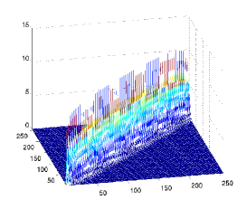
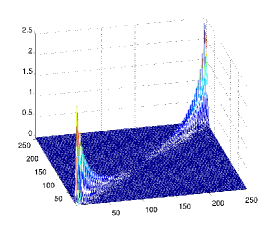
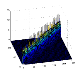
Figure 3.1: Matrix $V_{c_{L}}$ in a supercell for $L_{0}=3,L=32$ (left). Difference between matrices $V_{c_{L}}$ in periodic and single-box cases (middle). Block-sparsity in the matrix $V_{c_{L}}$ in periodic case (right).

Notice that the quantized approximation of canonical vectors involved in ${\bf G}_{k}$ and ${\bf P}_{c_{L}}$ reduces this cost to the logarithmic scale, $O(M_{0}R_{\cal N}\log N_{L})$, that is important in the case of large $L$ in view of $N_{L}=O(L)$.

The block $L_{0}$-diagonal structure of the matrix $V_{c_{L}}=\{V_{{\bf k}{\bf m}}\}$, ${\bf k}\in\mathbb{Z}^{3}$ ($-L/2\leq{k}_{\ell}L/2$) described by Lemma 3.1 allows the essential saving in the storage costs.

However, the polynomial complexity scaling in $L$ leads to severe limitations on the number of unit cells. These limitations can be relax if we look more precisely on the defect between matrix ${V}_{c_{L}}$ and its block-circulant version corresponding to the periodic boundary conditions (see §4.1). This defect can be split into two components with respect to their local and non-local features:

1. Non-local effect due to the asymmetry in the interaction potential sum on the lattice in a box.

2. The near boundary (local) defect that effects only those blocks in $V_{c_{L}}=\{V_{{\bf k}{\bf m}}\}$ lying in the $L_{0}$-width of $\partial\Omega_{L}$,

   $$L_{0}+1-(L-1)/2\leq k_{\ell},m_{\ell}\leq(L-1)/2-1-L_{0}.$$

Item (A) is related to a slight modification of the core potential to the shift invariant Toeplitz-type form $V_{{\bf k}{\bf m}}=V_{|{\bf k}-{\bf m}|}$ by replication of the central block corresponding to $k=0$, as considered in the next section. In this way the overlap condition (3.13) for the tensor ${\bf G}_{\bf k}$ will impose the block sparsity.

The boundary effect in item (B) becomes relatively small for large number of cells so that the block-circulant part of the matrix $V_{c_{L}}$ is getting dominating as $L\to\infty$.

The full diagonalization for above mentioned matrices is impossible. However the efficient storage and fast matrix-times-vector algorithms can be applied in the framework of iterative methods for calculation of a small subset of eigenvalues.

3.4 Discrete Laplacian and the mass matrix

The Laplace operator part included in eigenvalue problem for a single molecule is posed in the unit cell $\Omega=[-b/2,b/2]^{3}\in\mathbb{R}^{3}$, subject to the homogeneous Dirichlet boundary conditions on $\partial\Omega$. In periodic case they should be substituted by the periodic boundary conditions. For given discretization parameter $\overline{n}\in\mathbb{N}$, we use the equidistant $\overline{n}\times\overline{n}\times\overline{n}$ tensor grid $\omega_{{\bf 3},\overline{n}}=\{x_{\bf i}\}$, ${\bf i}\in{\cal I}:=\{1,...,\overline{n}\}^{3}$, with the mesh-size $h=2b/(\overline{n}+1)$, which might be different from the grid $\omega_{{\bf 3},n}$ introduced for representation of the interaction potential (usually, $n\leq\overline{n}$).

Define a set of piecewise linear basis functions $\overline{g}_{k}:={\bf I}_{1}g_{k}$, $k=1,...,N_{b}$, by linear tensor-product interpolation via the set of product hat functions, $\{\xi_{\bf i}\}=\xi_{i_{1}}(x_{1})\xi_{i_{2}}(x_{2})\xi_{i_{3}}(x_{3})$, ${\bf i}\in{\cal I}$, associated with the respective grid-cells in $\omega_{{\bf 3},N}$. Here the linear interpolant ${\bf I}_{1}={I}_{1}\times{I}_{1}\times{I}_{1}$ is a product of 1D interpolation operators, $\overline{g}_{k}^{(\ell)}={I}_{1}{g}_{k}^{(\ell)}$, $\ell=1,...,3$, where ${I}_{1}:C^{0}([-b,b])\to W_{h}:=span\{\xi_{i}\}_{i=1}^{\overline{n}}$ is defined over the set of piecewise linear basis functions by

$$({I}_{1}\,w)(x_{\ell}):=\sum_{i=1}^{\tilde{n}}w(x_{i_{\ell}})\xi_{i}(x_{\ell}),\quad x_{\bf i}\in\omega_{{\bf 3},\tilde{n}}.$$

With these definitions, the rank-$3$ tensor representation of the standard FEM Galerkin stiffness matrix for the Laplacian, $A_{3}$, in the tensor basis $\{\xi_{i}(x_{1})\xi_{j}(x_{2})\xi_{k}(x_{3})\}$, $i,j,k=1,\ldots\overline{n}$, is given by

$$A_{3}:=A^{(1)}\otimes S^{(2)}\otimes S^{(3)}+S^{(1)}\otimes A^{(2)}\otimes S^{(3)}+S^{(1)}\otimes S^{(2)}\otimes A^{(3)}\in\mathbb{R}^{\overline{n}^{\otimes 3}\times\overline{n}^{\otimes 3}},$$

where the 1D stiffness and mass matrices $A^{(\ell)},S^{(\ell)}\in\mathbb{R}^{\overline{n}\times\overline{n}}$, $\ell=1,\,2,\,3$, are represented by

$$A^{(\ell)}:=\{\langle\frac{d}{dx_{\ell}}\xi_{i}(x_{\ell}),\frac{d}{dx_{\ell}}\xi_{j}(x_{\ell})\rangle\}^{\overline{n}}_{i,j=1}=\frac{1}{h}\mbox{tridiag}\{-1,2,-1\},$$

$$S^{(\ell)}=\{\langle\xi_{i},\xi_{j}\rangle\}^{\overline{n}}_{i,j=1}=\frac{h}{6}\;\mbox{tridiag}\{1,4,1\},$$

respectively.

This leads to the separable grid-based approximation of the initial basis functions $g_{k}(x)$,

$$g_{k}(x)\approx\overline{g}_{k}(x)=\prod^{3}_{\ell=1}\overline{g}_{k}^{(\ell)}(x_{\ell})=\prod^{3}_{\ell=1}\sum\limits^{\overline{n}}_{i=1}g_{k}^{(\ell)}(x_{i_{\ell}})\xi_{i}(x_{\ell}),$$ (3.14)

where the rank-$1$ coefficients tensor ${\bf G}_{k}$ is given by ${\bf G}_{k}={\bf g}_{k}^{(1)}\otimes{\bf g}_{k}^{(2)}\otimes{\bf g}_{k}^{(3)}$, with the canonical vectors ${\bf g}_{k}^{(\ell)}=\{g_{k_{i}}^{(\ell)}\}\equiv\{g_{k}^{(\ell)}(x_{i_{\ell}})\}$. Let us agglomerate the rank-$1$ tensors ${\bf G}_{k}\in\mathbb{R}^{{\overline{n}}^{\otimes 3}}$, ($k=1,...,N_{b}$) in a tensor-valued matrix $G\in\mathbb{R}^{N^{\otimes 3}\times N_{b}}$, the Galerkin matrix in the basis set ${\bf G}_{k}$ can be written in a matrix form

$$A_{G}=G^{T}A_{3}G\in\mathbb{R}^{N_{b}\times N_{b}},$$

corresponding to the standard matrix-matrix transform under the change of basis. The matrix entries in $A_{G}=\{a_{km}\}$ can be represented by

$$a_{km}=\langle A_{3}{\bf G}_{k},{\bf G}_{m}\rangle,\quad k,m=1,...,N_{b}.$$

Likewise, for the entries of the stiffness matrix we have $s_{km}=\langle{\bf G}_{k},{\bf G}_{m}\rangle$.

It is easily seen that in the periodic case both matrices, $A_{G}$ and $S$, take the multilevel block circulant structure.

4 Linearized spectral problem by FFT-diagonalization

There are two possibilities for mathematical modeling of the $L$-periodic molecular systems, composed, of $(L,L,L)$ elementary unit cells. In the first approach, the system is supposed to contain an infinite set of equivalent atoms that map identically into itself under any translation by $L$ units in each spacial direction. The other model is based on the ring-type periodic structures consisting of $L$ identical units in each spacial direction, where every unit cell of the periodic compound will be mapped to itself by applying a rotational transform from the corresponding rotational group symmetry [39].

The main difference between these two concepts is in the treatment of the lattice sum of Coulomb interactions, thought, in the limit of $L\to\infty$ both models approach each other. In this paper we mainly follow the first approach with the particular focus on the asymptotic complexity optimization for large lattice parameter $L$. The second concept is useful for understanding the block structure of the Galerkin matrices for Laplacian and the identity operators.

4.1 Block circulant structure of core Hamiltonian in periodic case

Inthis section we consider the periodic case, further called case (P), and derive the more refined sparsity pattern of the matrix $V_{c_{L}}$ using the $d$-level ($d=1,2,3$) tensor structure in this matrix. The matrix block entries are numbered by a pair of multi-indices, $V_{c_{L}}=\{V_{{\bf k}{\bf m}}\}$, ${\bf k}=(k_{1},k_{2},k_{3})$, where the $m_{0}\times m_{0}$ matrix block $V_{{\bf k}{\bf m}}$ is defined by (3.11). Figure 4.1 illustrates an example of 3D lattice-type structure of size $(4,4,2)$.

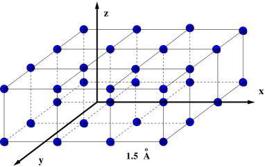
Figure 4.1: Example of the 3D lattice-type structure of size $(4,4,2)$.

Following [28] we introduce the periodic cell ${\cal R}=\mathbb{Z}^{d}$, $d=1,2,3$ for the $\bf k$ index, and consider a 3D $B$-periodic supercell $\Omega_{L}=B\times B\times B$, with $B=\frac{b}{2}[-L,L]$. The total electrostatic potential in the supercell $\Omega_{L}$ is obtained by, first, the lattice summation of the Coulomb potentials over $\Omega_{L}$ for (rather large) $L$, but restricted to the central unit cell $\Omega_{0}$, and then by replication of the resultant function to the whole supercell. Hence, that the total potential sum $v_{c_{L}}(x)$ is designated at each elementary unit-cell in $\Omega_{L}$ by the same value (${\bf k}$-translation invariant). The effect of the conditional convergence of the lattice summation can be treated by using the extrapolation to the limit (regularization) on a sequence of different lattice parameters $L$ as described in [28].

The electrostatic potential in any of $B$-periods can be obtained by copying the respective data from $\Omega_{L}$. The basis set in $\Omega_{L}$ is constructed by replication from the the master unit cell $\Omega_{0}$ over the whole periodic lattice.

Consider the case $d=3$ in more detail. Recall that the reference value $v_{c_{L}}(x)$ will be computed at the central cell $\Omega_{0}$, indexed by $(0,0,0)$, by summation over all contributions from $L^{3}$ elementary sub-cells in $\Omega_{L}$. For technical reasons here and in the following we vary the summation index in $k_{\ell}=0,...,L-1$ and obtain

$$v_{0}(x)=\sum_{\nu=1}^{M_{0}}\sum\limits_{k_{1},k_{2},k_{3}=0}^{L-1}\frac{Z_{\nu}}{\|{x}-a_{\nu}(k_{1},k_{2},k_{3})\|},\quad x\in\Omega_{0}.$$ (4.1)

The local lattice sum on the index set $n\times n\times n$ corresponding to $\Omega_{0}$, is represented by

$${\bf P}_{\Omega_{0}}=\sum_{\nu=1}^{M_{0}}Z_{\nu}\sum\limits_{k_{1},k_{2},k_{3}=0}^{L-1}\sum\limits_{q=1}^{R_{\cal N}}{\cal W}_{\nu({\bf k})}\widetilde{\bf p}^{(1)}_{q}\otimes\widetilde{\bf p}^{(2)}_{q}\otimes\widetilde{\bf p}^{(3)}_{q}\in\mathbb{R}^{n\times n\times n},$$

for the corresponding local projected tensor of small size $n\times n\times n$. Here the $\Omega$-windowing operator, ${\cal W}_{\nu({\bf k})}={\cal W}_{\nu(k_{1})}^{(1)}\otimes{\cal W}_{\nu(k_{2})}^{(2)}\otimes{\cal W}_{\nu(k_{3})}^{(3)},$ restricts onto the small $n\times n\times n$ unit cell by shifting by the lattice vector ${\bf k}=(k_{1},k_{2},k_{3})$. This reduces both the computational and storage costs by factor $L$.

In the 3D case, we set $q=3$ in the notation for multilevel BC matrix. Similar to the case of one-level BC matrices, we notice that a matrix $A\in{\cal BC}(3,{\bf L},m)$ of size $|{\bf L}|m\times|{\bf L}|m$ is completely defined by a $3$-rd order coefficients tensor ${\bf A}=[A_{k_{1}k_{2}k_{3}}]$ of size $L_{1}\times L_{2}\times L_{3}$, ($k_{\ell}=0,...,L_{\ell}-1$, $\ell=1,2,3$), with $m\times m$ block-matrix entries, obtained by folding of the generating first column vector in $A$.

Lemma 4.1

Assume that in case (P) the number of overlapping unit cells (in the sense of supports of basis functions) in each spatial direction does not exceed $L_{0}$. Then the Galerkin matrix $V_{c_{L}}$ exhibits the symmetric, three-level block circulant Kronecker tensor-product form. i.e. $V_{c_{L}}\in{\cal BC}(3,{\bf L},m_{0})$, (${\bf L}=(L_{1},L_{2},L_{3})$)

$$V_{c_{L}}=\sum\limits_{k_{1}=0}^{L_{1}-1}\sum\limits_{k_{2}=0}^{L_{2}-1}\sum\limits_{k_{3}=0}^{L_{3}-1}\pi_{L_{1}}^{k_{1}}\otimes\pi_{L_{2}}^{k_{2}}\otimes\pi_{L_{3}}^{k_{3}}\otimes A_{k_{1}k_{2}k_{3}},\quad A_{k_{1}k_{2}k_{3}}\in\mathbb{R}^{m_{0}\times m_{0}},$$ (4.2)

where the number non-zero matrix blocks $A_{k_{1}k_{2}k_{3}}$ does not exceed $(L_{0}+1)^{3}$.

The required storage is bounded by $m_{0}^{2}[(L_{0}+1)]^{3}$ independent of $L$. The set of non-zero generating matrix blocks $\{A_{k_{1}k_{2}k_{3}}\}$ can be calculated in $O(m_{0}^{2}[(L_{0}+1)]^{3}n)$ operations.

Furthermore, assume that the QTT ranks of the assembled canonical vectors do not exceed $r_{0}$. Then the numerical cost can be reduced to the logarithmic scale, $O(m_{0}^{2}[(L_{0}+1)]^{3}\log n)$.

Proof. First, we notice that the shift invariance property in the matrix $V_{c_{L}}=\{V_{{\bf k}{\bf m}}\}$ is a consequence of the translation invariance in the canonical tensor ${\bf P}_{c_{L}}$ (periodic case), and in the basis-tensor ${\bf G}_{\bf k}$ (by construction),

$${\bf G}_{\bf km}:={\bf G}_{\bf k}\odot{\bf G}_{\bf m}={\bf G}_{|{\bf k}-{\bf m}|}\quad\mbox{for}\quad|k_{\ell}|,|m_{\ell}|\leq L-1,$$ (4.3)

so that we have

$$V_{{\bf k}{\bf m}}=V_{|{\bf k}-{\bf m}|},\quad 0\leq k_{\ell},m_{\ell}\leq L-1.$$ (4.4)

This ensures the perfect three-level block-Toeplitz structure of $V_{c_{L}}$ (compare with the case of a box). Now the block circulant pattern in ${\cal BC}(3,{\bf L},m_{0})$ is imposed by the periodicity of a lattice-structured basis set.

To prove the complexity bounds we observe that a matrix $V_{c_{L}}\in{\cal BC}(3,{\bf L},m_{0})$ can be represented in the Kronecker tensor product form (4.2), obtained by an easy generalization of (6.2). In fact, we apply (6.2) by successive slice-wise and fiber-wise splitting to obtain

$$\begin{split}V_{c_{L}}&=\sum\limits_{k_{1}=0}^{L_{1}-1}\pi_{L_{1}}^{k_{1}}\otimes{\bf A}_{k_{1}}\\ &=\sum\limits_{k_{1}=0}^{L_{1}-1}\pi_{L_{1}}^{k_{1}}\otimes\left(\sum\limits_{n_{2}=0}^{L_{2}-1}\pi_{L_{2}}^{k_{2}}\otimes{\bf A}_{k_{1}k_{2}}\right)\\ &=\sum\limits_{k_{1}=0}^{L_{1}-1}\pi_{L_{1}}^{k_{1}}\otimes\left(\sum\limits_{k_{2}=0}^{L_{2}-1}\pi_{L_{2}}^{k_{2}}\otimes\left(\sum\limits_{k_{3}=0}^{L_{3}-1}\pi_{L_{3}}^{k_{3}}\otimes{A}_{k_{1}k_{2}k_{3}}\right)\right),\end{split}$$

where ${\bf A}_{k_{1}}\in\mathbb{R}^{L_{2}\times L_{3}\times m_{0}\times m_{0}}$, ${\bf A}_{k_{1}k_{2}}\in\mathbb{R}^{L_{3}\times m_{0}\times m_{0}}$, and $A_{k_{1}k_{2}k_{3}}\in\mathbb{R}^{m_{0}\times m_{0}}$. Now the overlapping assumption ensures that the number of non-zero matrix blocks $A_{k_{1}k_{2}k_{3}}$ does exceed $(L_{0}+1)^{3}$.

Furthermore, the symmetric mass matrix, $S_{c_{L}}=\{{s}_{\mu\nu}\}\in\mathbb{R}^{N_{b}\times N_{b}}$, for the Galerkin representation of the identity operator reads as follows,

$${s}_{\mu\nu}=\langle{\bf G}_{\mu},{\bf G}_{\nu}\rangle=\langle S^{(1)}{\bf g}_{\mu}^{(1)},{\bf g}_{\nu}^{(1)}\rangle\langle S^{(2)}{\bf g}_{\mu}^{(2)},{\bf g}_{\nu}^{(2)}\rangle\langle S^{(3)}{\bf g}_{\mu}^{(3)},{\bf g}_{\nu}^{(3)}\rangle,\quad 1\leq\mu,\nu\leq N_{b},$$

where $N_{b}=m_{0}L^{3}$. It can be seen that in the periodic case the block structure in the basis-tensor ${\bf G}_{\bf k}$ imposes the three-level block circulant structure in the mass matrix $S_{c_{L}}$

$$S_{c_{L}}=\sum\limits_{k_{1}=0}^{L_{1}-1}\sum\limits_{k_{2}=0}^{L_{2}-1}\sum\limits_{k_{3}=0}^{L_{3}-1}\pi_{L_{1}}^{k_{1}}\otimes\pi_{L_{2}}^{k_{2}}\otimes\pi_{L_{3}}^{k_{3}}\otimes S_{k_{1}k_{2}k_{3}},\quad S_{k_{1}k_{2}k_{3}}\in\mathbb{R}^{m_{0}\times m_{0}}.$$ (4.5)

By the previous arguments we conclude that $S_{k_{1}k_{2}k_{3}}=S^{(1)}_{k_{1}}S^{(2)}_{k_{2}}S^{(3)}_{k_{3}}$ implying the rank-$1$ separable representation in (4.5).

Likewise, it is easy to see that the stiffness matrix representing the (local) Laplace operator in the periodic setting has the similar block circulant structure,

$$\Delta_{c_{L}}=\sum\limits_{k_{1}=0}^{L_{1}-1}\sum\limits_{k_{2}=0}^{L_{2}-1}\sum\limits_{k_{3}=0}^{L_{3}-1}\pi_{L_{1}}^{k_{1}}\otimes\pi_{L_{2}}^{k_{2}}\otimes\pi_{L_{3}}^{k_{3}}\otimes B_{k_{1}k_{2}k_{3}},\quad B_{k_{1}k_{2}k_{3}}\in\mathbb{R}^{m_{0}\times m_{0}},$$ (4.6)

where the number non-zero matrix blocks $B_{k_{1}k_{2}k_{3}}$ does not exceed $(L_{0}+1)^{3}$. In this case the matrix block $B_{k_{1}k_{2}k_{3}}$ admits a rank-$3$ product factorization.

This proves the sparsity pattern of our tensor approximation to $H$.   

In the Hartree-Fock calculations for lattice structured systems we deal with the multilevel, symmetric block circulant/Toeplitz matrices, where the first-level blocks, $A_{0},...,A_{L_{1}-1}$, may have further block structures. In particular, Lemma 4.1 shows that the Galerkin approximation of the 3D Hartree-Fock core Hamiltonian in periodic setting leads to the symmetric, three-level block circulant matrix.

Figure 4.2 represents the block-sparsity in the core Hamiltonian matrix in a box for $L=8$ (left), and the rotated matrix profile (right).

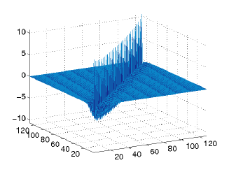
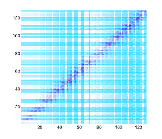
Figure 4.2: Block-sparsity in the core Hamiltonian matrix in a box for $L=8$ (left); Rotated matrix profile (right).

In the next section we discuss computational details of the FFT-based eigenvalue solver on the example of 3D linear chain of molecules.

4.2 Regularized spectral problem and complexity analysis

Combining the block circulant representations (4.2), (4.6) and (4.5), we are able to represent the eigenvalue problem for the Fock matrix in the Fourier space as follows

$$\sum\limits^{L_{1}-1}_{k_{1}=0}\sum\limits^{L_{2}-1}_{k_{2}=0}\sum\limits^{L_{3}-1}_{k_{3}=0}D_{L_{1}}^{k_{1}}\otimes D_{L_{2}}^{k_{2}}\otimes D_{L_{3}}^{k_{3}}\otimes(B_{k_{1}k_{2}k_{3}}+A_{k_{1}k_{2}k_{3}})U=\lambda\sum\limits^{L_{1}-1}_{k_{1}=0}\sum\limits^{L_{2}-1}_{k_{2}=0}\sum\limits^{L_{3}-1}_{k_{3}=0}D_{L_{1}}^{k_{1}}\otimes D_{L_{2}}^{k_{2}}\otimes D_{L_{3}}^{k_{3}}S_{k_{1}k_{2}k_{3}}U,$$

with the diagonal matrices $D_{L_{\ell}}^{k_{\ell}}\in\mathbb{R}^{L_{\ell}\times L_{\ell}}$, $\ell=1,2,3$, where $U=F_{\bf L}\otimes I_{m}C$. The equivalent block-diagonal form reads

$$\mbox{bdiag}_{m_{0}\times m_{0}}\{{\cal T}_{\bf L}^{\prime}[F_{\bf L}({\cal T}_{\bf L}\widehat{B})+F_{\bf L}({\cal T}_{\bf L}\widehat{A})]-\lambda{\cal T}_{\bf L}^{\prime}(F_{\bf L}[{\cal T}_{\bf L}\widehat{S})]\}U=0.$$ (4.7)

The block structure specified by Lemma 4.1 allows to apply the efficient eigenvalue solvers via FFT based diagonalization in the framework of Hartree-Fock calculations, in general, with the numerical cost $O(m_{0}^{2}L^{d}\log L)$.

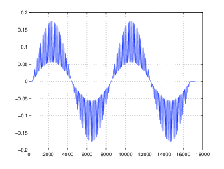
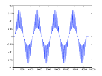
Figure 4.3: Molecular orbitals, i.e. the eigenvectors represented in GTO basis: the $4$th orbital (left), the $8$th orbital (right).

Proposition 4.2

The low-rank structure in the coefficients tensor mentioned above (see Section 2.2) allows to reduce the factor $L^{d}\log L$ to $L\log L$ for $d=2,3$. It was already observed in the proof of Lemma 4.1 that the respective coefficients in the overlap and Laplacian Galerkin matrices can be treated as the rank-$1$ and rank-$3$ tensors, respectively. Clearly, the factorization rank for the nuclear part of the Hamiltonian does not exceed $R_{\cal N}$. Hence, Theorem 2.5 can be applied in generalized form.

Figure 4.3 visualizes molecular orbitals on fine spatial grid with $n=2^{14}$: the $4$th orbital (left), the $8$th orbital (right). The eigenvectors are computed in GTO basis for $(L,1,1)$ system with $L=128$ and $m_{0}=4$.

Table 4.1 compares CPU times in sec. (Matlab) for the full eigenvalue solver on a 3D $(L,1,1)$ lattice in a box, and for the FTT-based diagonalization in the periodic supercell, all computed for $m_{0}=4$, $L=2^{p}$ ($p=7,8,...,15$). The number of basis function (problem size) is given by $N_{b}=m_{0}L$.

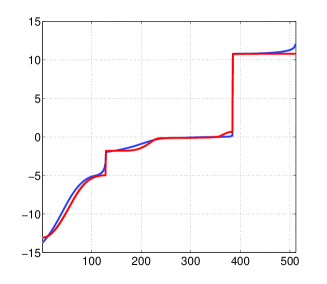
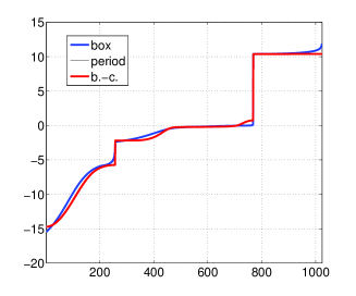
Figure 4.4: Spectrum of the core Hamiltonian.

Problem size $N_{b}=n_{0}L$	$512$	$1024$	$2048$	$4096$	$8192$	$16384$	$32768$	$65536$	$131072$
Full EIG-solver	$0.67$	$5.49$	$48.6$	$497.4$	$--$	$--$	$--$	$--$	$--$
FFT diagonalization	$0.10$	$0.09$	$0.08$	$0.14$	$0.44$	$1.5$	$5.6$	$22.9$	$89.4$

Table 4.1: CPU times (sec.): full eig-solver vs. FFT-based diagonalization for $(L,1,1)$ lattice, and with $m_{0}=4$, $L=2^{p}$, $p=7,8,...,15$.

Figure 4.4 represents the spectrum of the core Hamiltonian in a box vs. those in a periodic supercell for different number of cells $L=128,256$, where $m_{0}=4$. The systematic difference between the eigenvalues in both cases can be observed even for very large $L$. This spectral pollution effects have been discussed and theoretically analyzed in [6].

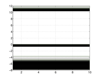
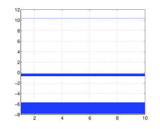
Figure 4.5: Spectrum of the core Hamiltonian for a $(L,1,1)$ lattice with $L=256$, and $m_{0}=4$, in a box (left) and for periodic case (right).

Figure 4.5 presents the spectral bands for a $(L,1,1)$ lattice system in a box and in the periodic setting, for $L=256$, and $m_{0}=4$.

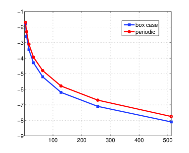
Figure 4.6: Average energy per unit cell vs. $L$ for a $(L,1,1)$ lattice in a 3D rectangular “tube“.

Figure 4.6 demonstrates the relaxation of the average energy per unit cell with $m_{0}=4$, for a $(L,1,1)$ lattice structure in a 3D rectangular “tube‘ up to $L=512$, for both periodic and open boundary conditions.

5 Conclusions

We have introduced and analyzed the grid-based tensor product approach to discretization and solution of the Hartree-Fock equation in ab initio modeling of the lattice-structured molecular systems. In this presentation we consider the case of core Hamiltonian. All methods and algorithms developed in this paper are implemented and tested in Matlab.

The proposed tensor techniques manifest the twofold benefits: (a) the entries of the Fock matrix are computed by 1D operations using low-rank tensors represented on a 3D grid, (b) the low-rank tensor structure in the diagonal blocks of the Fock matrix in the Fourier space reduces the conventional 3D FFT to the product of 1D Fourier transforms. The main contributions include:

• Fast computation of Fock matrix by 1D matrix-vector operations using low-rank tensors represented on a 3D spacial grid.

• Analysis and numerical implementation of the multilevel block circulant representation of the Fock matrix in the periodic setting.

• Investigation of the low-rank tensor structure in the diagonal blocks of the Fock matrix represented in the Fourier space, that allows to reduce the conventional 3D FFT to the product of 1D FFTs.

• Numerical tests illustrating the computational efficiency of the tensor-structured methods applied to the reduced Hartree-Fock equation for lattice-type and periodic systems. Numerical experiments on verification of the theoretical results on the asymptotic complexity estimated of the presented algorithms.

Here we confine ourself to the case of core Hamiltonian part in the full Fock matrix (linear part in the Fock operator). The rigorous study of the fully nonlinear self-consistent Hartree-Fock eigenvalue problem for periodic and lattice-structured systems in a box is a matter of future research.

6 Appendix: Overview on block circulant matrices

We recall that a one-level block circulant matrix $A\in{\cal BC}(L,m_{0})$ is defined by [8],

$$A=\operatorname{bcirc}\{A_{0},A_{1},...,A_{L-1}\}=\begin{bmatrix}A_{0}&A_{L-1}&\cdots&A_{2}&A_{1}\\ A_{1}&A_{0}&\cdots&\vdots&A_{2}\\ \vdots&\vdots&\ddots&A_{0}&\vdots\\ A_{L-1}&A_{L-2}&\cdots&A_{1}&A_{0}\\ \end{bmatrix}\in\mathbb{R}^{Lm_{0}\times Lm_{0}},$$ (6.1)

where $A_{k}\in\mathbb{R}^{m_{0}\times m_{0}}$ for $k=0,1,\ldots,L-1$, are matrices of general structure. The equivalent Kronecker product representation is defined by the associated matrix polynomial,

$$A=\sum\limits^{L-1}_{k=0}\pi^{k}\otimes A_{k}=:p_{A}(\pi),$$ (6.2)

where $\pi=\pi_{L}\in\mathbb{R}^{L\times L}$ is the periodic downward shift (cycling permutation) matrix,

$$\pi_{L}:=\begin{bmatrix}0&0&\cdots&0&1\\ 1&0&\cdots&0&0\\ \vdots&\vdots&\ddots&\vdots&\vdots\\ 0&\cdots&1&0&0\\ 0&0&\cdots&1&0\\ \end{bmatrix},$$ (6.3)

and $\otimes$ denotes the Kronecker product of matrices.

In the case $m_{0}=1$ a matrix $A\in{\cal BC}(L,1)$ defines a circulant matrix generated by its first column vector $\widehat{a}=(a_{0},...,a_{L-1})^{T}$. The associated scalar polynomial then reads

$$p_{A}(z):=a_{0}+a_{1}z+...+a_{L-1}z^{L-1},$$

so that (6.2) simplifies to

$$A=p_{A}(\pi_{L}).$$

Let $\omega=\omega_{L}=\exp(-\frac{2\pi i}{L})$, we denote by

$$F_{L}=\{f_{k\ell}\}\in\mathbb{R}^{L\times L},\quad\mbox{with}\quad f_{k\ell}=\frac{1}{\sqrt{L}}\omega_{L}^{(k-1)(\ell-1)},\quad k,l=1,...,L,$$

the unitary matrix of Fourier transform. Since the shift matrix $\pi_{L}$ is diagonalizable in the Fourier basis,

$$\pi_{L}=F_{L}^{\ast}D_{L}F_{L},\quad D_{L}=\mbox{diag}\{1,\omega,...,\omega^{L-1}\},$$ (6.4)

the same holds for any circulant matrix,

$$A=p_{A}(\pi_{L})=F_{L}^{\ast}p_{A}(D_{L})F_{L},$$ (6.5)

where

$$p_{A}(D_{L})=\mbox{diag}\{p_{A}(1),p_{A}(\omega),...,p_{A}(\omega^{L-1})\}=\mbox{diag}\{F_{L}a\}.$$

Conventionally, we denote by $\mbox{diag}\{x\}$ a diagonal matrix generated by a vector $x$. Let $X$ be an $Lm_{0}\times m_{0}$ matrix obtained by concatenation of $m_{0}\times m_{0}$ matrices $X_{k}$, $k=0,...,L-1$, $X=\operatorname{conc}(X_{0},...,X_{L-1})=[X_{0},...,X_{L-1}]^{T}$. For example, the first block column in (6.1) has the form $\operatorname{conc}(A_{0},...,A_{L-1})$. We denote by $\mbox{bdiag}\{X\}$ the $Lm_{0}\times Lm_{0}$ block-diagonal matrix of block size $L$ generated by $m_{0}\times m_{0}$ blocks $X_{k}$.

It is known that similarly to the case of circulant matrices (6.5), block circulant matrix in ${\cal BC}(L,m_{0})$ is unitary equivalent to the block diagonal one by means of Fourier transform via representation (6.2), see [8]. In the following, we describe the block-diagonal representation of a matrix $A\in{\cal BC}(L,m_{0})$ in the form that is convenient for generalization to the multi-level block circulants as well as for the description of FFT based implementational schemes. To that end, let us introduce the reshaping (folding) transform ${\cal T}_{L}$ that maps a $Lm_{0}\times m_{0}$ matrix $X$ (i.e., the first block column in $A$) to $L\times m_{0}\times m_{0}$ tensor $B={\cal T}_{L}X$ by plugging the $i$th $m_{0}\times m_{0}$ block in $X$ into a slice $B(i,:,:)$. The respective unfolding returns the initial matrix $X={\cal T}_{L}^{\prime}B$. We denote by $\widehat{A}\in\mathbb{R}^{Lm_{0}\times m_{0}}$ the first block column of a matrix $A\in{\cal BC}(L,m_{0})$, with a shorthand notation

$$\widehat{A}=[A_{0},A_{1},...,A_{L-1}]^{T},$$

so that the $L\times m_{0}\times m_{0}$ tensor ${\cal T}_{L}\widehat{A}$ represents slice-wise all generating $m_{0}\times m_{0}$ matrix blocks.

Proposition 6.1

For $A\in{\cal BC}(L,m_{0})$ we have

$$A=(F_{L}^{\ast}\otimes I_{m_{0}})\operatorname{bdiag}\{\bar{A}_{0},\bar{A}_{1},\ldots,\bar{A}_{L-1}\}(F_{L}\otimes I_{m_{0}}),$$ (6.6)

where

$$\bar{A}_{j}=\sum\limits^{L-1}_{k=0}\omega_{L}^{jk}A_{k}\in\mathbb{C}^{m_{0}\times m_{0}},$$

can be recognized as the $j$-th $m_{0}\times m_{0}$ matrix block in block column ${\cal T}_{L}^{\prime}(F_{L}({\cal T}_{L}\widehat{A}))$, such that

$$\left[\bar{A}_{0},\bar{A}_{1},\ldots,\bar{A}_{L-1}\right]^{T}={\cal T}_{L}^{\prime}(F_{L}({\cal T}_{L}\widehat{A})).$$

A set of eigenvalues $\lambda$ of $A$ is then given by

$$\{\lambda|Ax=\lambda x,\;x\in\mathbb{C}^{Lm_{0}}\}=\bigcup\limits_{j=0}^{L-1}\{\lambda|\bar{A}_{j}u=\lambda u,\;u\in\mathbb{C}^{m_{0}}\}.$$ (6.7)

The eigenvectors corresponding to the spectral sets

$$\Sigma_{j}=\{\lambda_{j,m}|\bar{A}_{j}u_{j,m}=\lambda_{j,m}u_{j,m},\;u_{j,m}\in\mathbb{C}^{m_{0}}\},\quad j=0,1,\ldots,L-1,\quad m=1,...,m_{0},$$

can be represented in the form

$$U_{j,m}=(F_{L}^{\ast}\otimes I_{m})\bar{U}_{j,m},\quad\mbox{where}\quad\bar{U}_{j,m}=E_{[j]}\operatorname{vec}\,[u_{0,m},u_{1,m},...,u_{L-1,m}],$$ (6.8)

with $E_{[j]}=\operatorname{diag}\{e_{j}\}\otimes I_{m_{0}}\in\mathbb{R}^{Lm_{0}\times Lm_{0}}$, and $e_{j}\in\mathbb{R}^{L}$ being the $j$th Euclidean basis vector.

Proof. We combine representations (6.2) and (6.4) to obtain

$$A =\sum\limits^{L-1}_{k=0}\pi^{k}\otimes A_{k}=\sum\limits^{L-1}_{k=0}(F_{L}^{\ast}D^{k}F_{L})\otimes A_{k}$$ (6.9)

$$=(F_{L}^{\ast}\otimes I_{m_{0}})(\sum\limits^{L-1}_{k=0}D^{k}\otimes A_{k})(F_{L}\otimes I_{m_{0}})$$

$$=(F_{n}^{\ast}\otimes I_{m})(\sum\limits^{L-1}_{k=0}\mbox{bdiag}\{A_{k},\omega_{L}^{k}A_{k},...,\omega_{L}^{k(L-1)}A_{k}\})(F_{L}\otimes I_{m_{0}})$$

$$=(F_{L}^{\ast}\otimes I_{m_{0}})\mbox{bdiag}\{\sum\limits^{L-1}_{k=0}A_{k},\sum\limits^{L-1}_{k=0}\omega_{L}^{k}A_{k},...,\sum\limits^{L-1}_{k=0}\omega_{L}^{k(L-1)}A_{k}\}(F_{L}\otimes I_{m_{0}})$$

$$=(F_{L}^{\ast}\otimes I_{m_{0}})\mbox{bdiag}_{m_{0}\times m_{0}}\{{\cal T}_{L}^{\prime}(F_{L}({\cal T}_{L}\widehat{A}))\}(F_{L}\otimes I_{m_{0}}),$$

where the final step follows by the definition of FT matrix and by the construction of ${\cal T}_{L}$. The structure of eigenvalues and eigenfunctions then follows by simple calculations with block-diagonal matrices.   

The next statement describes the block-diagonal form for a class of symmetric BC matrices, ${\cal BC}_{s}(L,m_{0})$, that is a simple corollary of [8], Proposition 6.1. In this case we have $A_{0}=A_{0}^{T}$, and $A_{k}^{T}=A_{L-k}$, $k=1,...,L-1$.

Corollary 6.2

Let $A\in{\cal BC}_{s}(L,m_{0})$ be symmetric, then $A$ is unitary similar to a Hermitian block-diagonal matrix, i.e., $A$ is of the form

$$A=(F_{L}\otimes I_{m_{0}})\operatorname{bdiag}(\tilde{A}_{0},\tilde{A}_{1},\ldots,\tilde{A}_{L-1})(F_{L}^{\ast}\otimes I_{m_{0}}),$$ (6.10)

where $I_{m_{0}}$ is the $m_{0}\times m_{0}$ identity matrix. The matrices $\tilde{A}_{j}\in\mathbb{C}^{m_{0}\times m_{0}}$, $j=0,1,\ldots,L-1$, are defined for even $n\geq 2$ as

$$\tilde{A}_{j}=A_{0}+\sum\limits^{L/2-1}_{k=1}(\omega^{kj}_{L}A_{k}+\overline{\omega}^{kj}_{L}A^{T}_{k})+(-1)^{j}A_{L/2}.$$ (6.11)

Corollary 6.2 combined with Proposition 6.1 describes a simplified structure of eigendata in the symmetric case. Notice that the above representation imposes the symmetry of each real-valued diagonal blocks $\tilde{A}_{j}\in\mathbb{R}^{m_{0}\times m_{0}},\;j=0,1,\ldots,L-1$, in (6.10).

Finally, we recall that a one-level symmetric block Toeplitz matrix $A\in{\cal BT}_{s}(L,m_{0})$ is defined by [8],

$$A=\operatorname{BToepl}_{s}\{A_{0},A_{1},...,A_{L-1}\}=\begin{bmatrix}A_{0}&A_{1}^{T}&\cdots&A_{L-2}^{T}&A_{L-1}^{T}\\ A_{1}&A_{0}&\cdots&\vdots&A_{L-2}^{T}\\ \vdots&\vdots&\ddots&A_{0}&\vdots\\ A_{L-1}&A_{L-2}&\cdots&A_{1}&A_{0}\\ \end{bmatrix}\in\mathbb{R}^{Lm_{0}\times Lm_{0}},$$ (6.12)

where $A_{k}\in\mathbb{R}^{m_{0}\times m_{0}}$ for $k=0,1,\ldots,L-1$, are matrices of a general structure.

References

• [1] Bloch, André, ”Les th or mes de M.Valiron sur les fonctions enti res et la th orie de l’uniformisation”. Annales de la facult des sciences de l’Universit de Toulouse 17 (3): 1-22 (1925). ISSN 0240-2963.
• [2] F.A. Bischoff and E.F. Valeev. Low-order tensor approximations for electronic wave functions: Hartree-Fock method with guaranteed precision. J. of Chem. Phys., 134, 104104-1-10 (2011).
• [3] C. Bertoglio, and B.N. Khoromskij. Low-rank quadrature-based tensor approximation of the Galerkin projected Newton/Yukawa kernels. Comp. Phys. Comm. 183(4) (2012) 904–912.
• [4] D. Braess. Nonlinear approximation theory. Springer-Verlag, Berlin, 1986.
• [5] D. Braess. Asymptotics for the Approximation of Wave Functions by Exponential-Sums. J. Approx. Theory, 83: 93-103, (1995).
• [6] E. Cancés, A. Deleurence and M. Lewin, A new approach to the modeling of local defects in crystals: The reduced Hartree-Fock case. Comm. Math. Phys. 281 (2008) 129-177.
• [7] E. Cancés, V. Ehrlacher, and Y. Maday. Periodic Schrödinger operator with local defects and spectral pollution. SIAM J. Numer. Anal. v. 50, No. 6 (2012), pp. 3016-3035.
• [8] J. P. Davis. Circulant matrices. New York. John Wiley & Sons, 1979.
• [9] S. Dolgov, B.N. Khoromskij, D. Savostyanov, and I. Oseledets. Computation of extreme eigenvalues in higher dimensions using block tensor train format. Comp. Phys. Communications, Volume 185, Issue 4, April 2014, 1207-1216. doi:10.1016/j.cpc.2013.12.017.
• [10] L. Frediani, E. Fossgaard, T. Flå and K. Ruud. Fully adaptive algorithms for multivariate integral equations using the non-standard form and multiwavelets with applications to the Poisson and bound-state Helmholtz kernels in three dimensions. Molecular Physics, v. 111, 9-11, 2013.
• [11] Y. Saad, J. R. Chelikowsky, and S. M. Shontz. Numerical Methods for Electronic Structure Calculations of Materials. SIAM Review, v. 52 (1), 2010, 3-54.
• [12] R. Dovesi, R. Orlando, C. Roetti, C. Pisani, and V.R. Sauders. The Periodic Hartree-Fock Method and its Implementation in the CRYSTAL Code. Phys. Stat. Sol. (b) 217, 63 (2000).
• [13] V. Ehrlacher, C. Ortner, and A. V. Shapeev. Analysis of boundary conditions for crystal defect atomistic simulations. e-prints ArXiv:1306.5334, 2013.
• [14] Ewald P.P. Die Berechnung optische und elektrostatischer Gitterpotentiale. Ann. Phys 64, 253 (1921).
• [15] I.P. Gavrilyuk, W. Hackbusch and B.N. Khoromskij. Hierarchical Tensor-Product Approximation to the Inverse and Related Operators in High-Dimensional Elliptic Problems. Computing 74 (2005), 131-157.
• [16] L. Grasedyck, D. Kressner and C. Tobler. A literature survey of low-rank tensor approximation techniques. arXiv:1302.7121v1, 2013.
• [17] W. Hackbusch and B.N. Khoromskij. Low-rank Kronecker product approximation to multi-dimensional nonlocal operators. Part I. Separable approximation of multi-variate functions. Computing 76 (2006), 177-202.
• [18] B.N. Khoromskij and V. Khoromskaia. Multigrid tensor approximation of function related multi-dimensional arrays. SIAM J. Sci. Comp. 31(4) (2009) 3002-3026.
• [19] B.N. Khoromskij, V. Khoromskaia, and H.-J. Flad. Numerical Solution of the Hartree-Fock Equation in Multilevel Tensor-structured Format. SIAM J. Sci. Comp. 33(1) (2011) 45-65.
• [20] V. Khoromskaia. Numerical Solution of the Hartree-Fock Equation by Multilevel Tensor-structured methods. PhD thesis, TU Berlin, 2010.
• [21] V. Khoromskaia, B.N. Khoromskij, and R. Schneider. Tensor-structured calculation of two-electron integrals in a general basis. SIAM J. Sci. Comput., 35(2), 2013, A987-A1010.
• [22] R.J. Harrison, G.I. Fann, T. Yanai, Z. Gan, and G. Beylkin. Multiresolution quantum chemistry: Basic theory and initial applications. J. of Chem. Phys. 121(23) (2004) 11587-11598.
• [23] D. R. Hartree. The Calculation of Atomic Structure, Wiley, New York, 1957.
• [24] Ch. Froese Fischer. The Hartree-Fock Method for Atoms – A Numerical Approach, Wiley, New York, 1977.
• [25] M.J. Frisch, G.W. Trucks, H.B. Schlegel, G.E. Scuseria, M.A. Robb, J.R. Cheeseman, G. Scalmani, V. Barone, B. Mennucci, G.A. Petersson et al., Gaussian development version Revision H.1, Gaussian Inc., Wallingford, CT, 2009.
• [26] E. A. McCullough, Jr. Numerical Hartree-Fock methods for molecules, in P. v. R. Schleyer et al. (eds.), Encyclopedia of Computational Chemistry (Vol. 3), Wiley, Chichester, (1998) 1941–1947.
• [27] T. Kailath, and A. Sayed. Fast reliable algorithms for matrices with structure. SIAM Publication, Philadelphia, 1999.
• [28] V. Khoromskaia and B. N. Khoromskij. Grid-based lattice summation of electrostatic potentials by assembled rank-structured tensor approximation. arXiv:1405.2270. CPC 2014, to appear.
• [29] B.N. Khoromskij. Tensors-structured Numerical Methods in Scientific Computing: Survey on Recent Advances. Chemometr. Intell. Lab. Syst. 110 (2012), 1-19.
• [30] T. G. Kolda and B. W. Bader. Tensor Decompositions and Applications. SIAM Rev. 51(3) (2009) 455–500.
• [31] W. Hackbusch, B.N. Khoromskij, S. Sauter, and E. Tyrtyshnikov. Use of tensor formats in elliptic eigenvalue problems. Numer. Lin. Alg. Appl., v. 19(1), 2012, 133-151.
• [32] B.N. Khoromskij. $O(d\log N)$-Quantics Approximation of $N$-$d$ Tensors in High-Dimensional Numerical Modeling. Constr. Approx. 34 (2011) 257–280.
• [33] H.-J. Werner, P.J. Knowles, et al. Molpro version 2010.1, A Package of Ab-Initio Programs for Electronic Structure Calculations.
• [34] T. Helgaker, P. Jørgensen, and J. Olsen. Molecular Electronic-Structure Theory. Wiley, New York, 1999.
• [35] V. Khoromskaia. Computation of the Hartree-Fock Exchange in the Tensor-structured Format. Comp. Meth. App. Math., 10(2) (2010) 204–218.
• [36] V. Khoromskaia. Black-box Hartree-Fock solver by tensor numerical methods. Comp. Meth. in Applied Math., vol. 14(2014) No. 1, pp.89-111.
• [37] T. H. Dunning, Jr. Gaussian basis sets for use in correlated molecular calculations. I. The atoms boron through neon and hydrogen, J. Chem. Phys. 90 (1989) 1007–1023.
• [38] Venera Khoromskaia. Numerical Solution of the Hartree-Fock Equation by Multilevel Tensor-structured methods. PhD thesis, TU Berlin, 2010.
http://opus4.kobv.de/opus4-tuberlin/frontdoor/index/index/docId/2780.
• [39] A. Szabo, and N. Ostlund. Modern Quantum Chemistry. Dover Publication, New York, 1996.
• [40] C. Pisani, M. Schütz, S. Casassa, D. Usvyat, L. Maschio, M. Lorenz, and A. Erba. CRYSCOR: a program for the post-Hartree-Fock treatment of periodic systems, Phys. Chem. Chem. Phys., 2012, 14, 7615-7628.
• [41] M. V. Rakhuba, I. V. Oseledets. Fast multidimensional convolution in low-rank formats via cross approximation. arXiv:1402.5649, 2013.
• [42] S. A. Losilla, D. Sundholm, J. Juselius The direct approach to gravitation and electrostatics method for periodic systems. J. Chem. Phys. 132 (2) (2010) 024102.
• [43] T. Blesgen, V. Gavini, V. Khoromskaia. Approximation of the electron density of Aluminium clusters in tensor-product format. J. Comp. Phys. 231(6) (2012) 2551–2564.
• [44] F. Stenger. Numerical methods based on Sinc and analytic functions. Springer-Verlag, 1993.