Multipolar universal relations between $f$-mode frequency and tidal deformability of compact stars

Abstract

Though individual stellar parameters of compact stars usually demonstrate obvious dependence on the equation of state (EOS), EOS-insensitive universal formulas relating these parameters remarkably exist. In the present paper, we explore the interrelationship between two such formulas, namely the $f$-$I$ relation connecting the $f$-mode quadrupole oscillation frequency $\omega_{2}$ and the moment of inertia $I$, and the $I$-Love-$Q$ relations relating $I$, the quadrupole tidal deformability $\lambda_{2}$, and the quadrupole moment $Q$, which have been proposed by Lau, Leung, and Lin [Astrophys. J. 714, 1234 (2010)] and Yagi and Yunes [Science 341, 365 (2013)], respectively. A relativistic universal relation between $\omega_{l}$ and $\lambda_{l}$ with the same angular momentum $l=2,3,\ldots$, the so-called “diagonal $f$-Love relation” that holds for realistic compact stars and stiff polytropic stars, is unveiled here. An in-depth investigation in the Newtonian limit is further carried out to pinpoint its underlying physical mechanism and hence leads to a unified $f$-$I$-Love relation. We reach the conclusion that these EOS-insensitive formulas stem from a common physical origin — compact stars can be considered as quasiincompressible when they react to slow time variations introduced by $f$-mode oscillations, tidal forces and rotations.

I Introduction

The structure of neutron stars (NSs), the remnants of supernovae, is dictated by the strong gravity prevailing inside such stars. As a result, the density of the inner core of a typical NS can be several times the normal nuclear density $2.8\times 10^{14}\,{\rm g\,cm}^{-3}$, which is not yet achievable (at least in a stable form) in the terrestrial environment. The equation of state (EOS) of nuclear matter in NSs is often masked by various uncertainties in nuclear and particle physics, leading to the associated uncertainties in the physical characteristics of NSs, including their masses, radii, and moments of inertia. Thus, it has become a common practice for nuclear physicists to examine how EOSs of high-density nuclear matter could affect the structure of NSs, e.g., the mass-radius relation, and systematic investigations along such direction have also been carried out (see, e.g., (Weber, 1999; Lattimer and Prakash, 2001; Lattimer and Schutz, 2005; Lattimer and Prakash, 2007)). On the other hand, mass efforts have been pooled together to infer the details of nuclear matter from various possibly detectable characteristics (such as mass, radius, moment of inertia and gravitational-wave spectrum) of NSs (see, e.g., (Andersson and Kokkotas, 1996, 1998; Lattimer and Prakash, 2001; Lattimer and Schutz, 2005; Lattimer and Prakash, 2007; Özel and Psaltis, 2009; Ho et al., 2013; Lattimer and Steiner, 2014; Lattimer and Lim, 2013)).

However, paralleling these attempts to differentiate the structure of NSs with respect to nuclear EOS and vice versa, several universal EOS-insensitive formulas connecting different physical parameters (e.g., mass, radius and moment of inertia) of NSs or quark stars (QSs) have also been discovered. Such formulas are important and useful as they enable astronomers to infer (or at least to constrain) a physical parameter of NSs (or QSs) from the others that are more amenable to physical measurement even in the absence of exact information of relevant EOSs. For example, Lattimer and Schutz Lattimer and Schutz (2005) and Bejger and Haensel Bejger and Haensel (2002) found formulas relating the moment of inertia $I$, the mass $M$, and the radius $R$ for NSs constructed with different realistic EOSs, which could be used to determine the moment of inertia of star A in the double pulsar system J0737-3039 (Burgay et al., 2003; Lyne et al., 2004) to about 10% accuracy. Besides, several universal behaviors of the quadrupolar $f$-mode oscillations of NSs have been established and applied to infer the EOS of nuclear matter (Andersson and Kokkotas, 1996, 1998; Benhar et al., 1999, 2004; Tsui and Leung, 2005a, b, c; Tsui et al., 2006; Lau et al., 2010), and similar studies have been extended to the quadrupolar and higher spherical order $f$-mode oscillations of rapidly rotating neutron stars (Gaertig and Kokkotas, 2011; Doneva et al., 2013)

It is particularly interesting to note that some of these universal formulas actually relate the dynamical response of a NS (or QS) under external perturbation to its static stellar structure. In particular, Lau, Leung, and Lin Lau et al. (2010) found that the frequency and damping rate of $f$-mode quadrupole oscillation are expressible in terms of $M$ and the effective compactness $\eta\equiv\sqrt{M^{3}/I}$, hereafter referred to as the “$f$-$I$ relations”. Hence, the values of $M$, $R$, and $I$ of a NS (or QS) can be inferred accurately from the $f$-mode gravitational-wave signals (Lau et al., 2010). Since pulsating NSs are expected to be promising sources of gravitational waves, the above-mentioned relations can lead to useful information about the static structure of NSs (or QSs) once the third-generation gravitational-wave detectors (e.g., the Einstein Telescope (Punturo et al., 2010)) are available in the future.

On the other hand, universal relations expressing the distortion of a NS induced by tidal forces or spin in terms of its static structural parameters have also been found recently (Yagi and Yunes, 2013a; Yagi and Yunes, 2013b; Urbanec et al., 2013; Baubock et al., 2013). The so-called “$I$-Love-$Q$ relations”, discovered by Yagi and Yunes Yagi and Yunes (2013a); Yagi and Yunes (2013b), relate $I$, the quadrupole tidal Love number $\lambda_{2}$ (or, more precisely, tidal deformability (Damour and Nagar, 2009; Yagi, 2014)), and the spin-induced quadrupole moment $Q$, with $M$ being a proper scaling parameter. The relations are robust and also prevail in several different situations, including binary systems with strong dynamical tidal field (Maselli et al., 2013), magnetized NSs with sufficiently high rotation rates (Haskell et al., 2014), and rapidly rotating stars (Pappas and Apostolatos, 2014; Chakrabarti et al., 2014). Besides, there are works extending the $I$-Love-$Q$ relations to consider the relation between higher-order multipole moments induced by either tidal forces or rotation (Yagi, 2014; Yagi et al., 2014; Stein et al., 2014).

Similar to other universal relations, these $I$-Love-$Q$ relations enable us to infer any two of $I$, $\lambda_{2}$ and $Q$ from the detected value of the remaining one even in the absence of prior knowledge of the EOS of NSs. In addition, the I-Love-Q relations could facilitate the analysis of gravitational-wave signals emitted during the late stages of NS-NS binary mergers (Flanagan and Hinderer, 2008; Hinderer, 2008; Yagi and Yunes, 2013a; Yagi and Yunes, 2013b), and also serve as an indicator to identify the validity of other modified gravity theories (Yagi and Yunes, 2013a; Yagi and Yunes, 2013b; Sham et al., 2014; Pani and Berti, 2014; Doneva et al., 2014; Kleihaus et al., 2014).

Despite the fact that the above-mentioned $f$-$I$ relation and $I$-Love-$Q$ relations were discovered separately, the moment of inertia $I$ is involved in both of them. It is physically natural to expect that there should be a link between these two relations. The present paper aims at examining their interrelationship and establishing universal relations that can directly link the characteristics of multipolar distortions induced respectively by oscillations and tidal forces together. First of all, we investigate the so-called “$f$-Love relation” between the $l$th multipolar f-mode oscillation frequency $\omega_{l}$ and the $l^{\prime}$th multipolar tidal deformability $\lambda_{l^{\prime}}$, where $l,l^{\prime}=2,3,4,\ldots$. We show that there exist approximately EOS-independent and relativistically correct relations between these two if $l=l^{\prime}$, which are referred to as the diagonal $f$-Love relations hereafter. It is obvious that the case with $l=2$ is a direct consequence of the original $f$-$I$ and $I$-Love-$Q$ relations (Yagi and Yunes, 2013a; Yagi and Yunes, 2013b; Lau et al., 2010). For the off-diagonal $f$-Love relations with $l\neq l^{\prime}$, the relation between the two relevant physical quantities become more EOS-sensitive (see Sec. III and Figs. 1-4). This finding is important and useful. On the one hand, assuming that the mass of a NS is known from astronomical measurements, one can use the diagonal $f$-Love relation to determine the f-mode frequency from the measured tidal deformability in the same angular momentum sector (Flanagan and Hinderer, 2008; Hinderer, 2008; Yagi and Yunes, 2013a; Yagi and Yunes, 2013b) (and vice versa) even in the absence of detailed knowledge of nuclear EOS. On the other, the details of EOS could be inferred from the off-diagonal $f$-Love relations.

To pursue the physical origin of the EOS-independency of the diagonal $f$-Love relations, we compare the $f$-Love relations of realistic stars and polytropic stars with those of incompressible stars (see Sec. III and Figs. 1-4). We find that the latter can nicely approximate the behavior of realistic stars (including both NSs and QSs) and polytropic stars whose polytropic indices $N$ are less than 1. As a matter of fact, the polytropic index of most (if not all) popular realistic nuclear EOSs in the high density regime is less than 1. Hence, these prevailing EOSs are stiff enough to guarantee the $f$-Love relations except for NSs with very low masses. If softer nuclear EOSs were proposed and used to construct NSs, such stars would demonstrate significant deviations from the $f$-Love relation discovered in the present paper. Conversely, if the $f$-Love relations were violated, it would hint at the softening of nuclear matter due to physical mechanisms such as kaon condensation or other phase transitions.

Furthermore, regarding the physical origin of the multipolar $f$-$I$, $I$-Love and $f$-Love formulas in the Newtonian limit, we consider a model star characterized by a density profile $\rho(r)=\rho_{0}(1-\delta x^{2})$ with $x\equiv r/R$ and $\rho_{0}$ being the central density (see Sec. IV A). Here $1\geq\delta\geq 0$ is a parameter controlling the stiffness of the star. With such a stellar model, we can approximately reproduce the behavior of QSs and NSs whose polytropic index is less than 1, while rendering calculations of physical quantities more manageable and simplified (see the discussion in Sec. IV A). First of all, we analytically derive the $f$-$I$ formula relating $\omega_{l}$ and $I_{n}$, where $I_{n}\equiv\int_{0}^{R}\rho(r)r^{2+n}\mathrm{d}r$ is the $n$th mass moment (see Sec. IV B), and the $I$-Love formula connecting $I_{n}$ and $\lambda_{l}$ (see Sec. IV C). In general, these two relations explicitly depend on the value of $\delta$, i.e., the underlying EOS of the star, and lack of universality. However, if $n=2l-2$, to first order in $\delta$ both of them are independent of $\delta$. Consequently, combining the $f$-$I$ and $I$-Love formulas, we can show that the diagonal $f$-Love formula is also to first order independent of $\delta$, corroborating the EOS independence of the diagonal $f$-Love formula discovered here (see Sec. IV D).

The analytic studies developed in the present paper clearly explain why these universal formulas are so insensitive to changes in EOSs. We arrive at the conclusion that the crux of the observed universality is (i) these universal relations actually derive from the behavior of incompressible stars; (ii) they are stationary with respect to changes in $N$ around the incompressible limit (i.e. $N=0$) and hence are EOS-insensitive; and (iii) the prevailing EOSs for nuclear matter are stiff enough to be considered as almost incompressible (termed as quasiincompressible here) in certain slow physical processes (e.g., $f$-mode oscillations, tidal and rotational deformation).

Physically speaking, if an external perturbation is applied to a compact star, the response of the star to such perturbation is given by the Green’s function, which consists of the contributions arising from different oscillation modes (Chandrasekhar, 1963; Press and Teukolsky, 1977). Tidal deformation of NSs is merely the zero-frequency component of the Green’s function. We show in the present paper that for quasiincompressible stars in the Newtonian limit, the tidal field couples only to the f-mode oscillation and establish a robust $f$-$I$-Love relation. Such a relation readily shows that the $f$-$I$ and $I$-Love relations imply each other, thus unifying these two independently discovered universal relations.

The plan of the paper is as follows. In Sec. II we briefly review the previously discovered universal behaviors of the quadrupole $f$-$I$ and $I$-Love-$Q$ relations for NSs. We present the multipolar $f$-Love universal relations in Sec. III and study how the stiffness of nuclear matter could affect the accuracy of the $f$-Love relation. Newtonian analytic analysis will be carried out in Sec. IV to establish the multipolar $f$-$I$, $I$-Love and $f$-Love relations. A unified Green’s function approach to multipolar tidal deformation in the Newtonian regime and hence a novel multipolar $f$-$I$-Love relation are given in Sec. V. The conclusions of the present paper are presented in Sec. VI. Unless otherwise stated explicitly, we use geometric units where $G=c=1$.

II Quadrupole $F$-$I$ and $I$-Love-$Q$ relations

When compact stars are perturbed away from their equilibrium state, their subsequent oscillations can be analyzed in terms of quasinormal modes (QNMs) (Press, 1971; Leaver, 1986; Ching et al., 1998; Kokkotas and Schmidt, 1999; Berti et al., 2009). Each QNM is characterized by a complex eigenfrequency $\omega=\omega_{\rm r}+i\omega_{\rm i}$, with $\omega_{\rm i}$ measuring its decay rate due to emission of gravitational waves. For typical NSs, the oscillation frequency $\omega_{\rm r}$ of the fundamental (f) mode usually lies in the kilohertz range, which is lower than other QNMs such as the pressure ($p$) modes and the spacetime (w) modes. Hence, as far as gravitational waves emitted from oscillating NSs are concerned, f-mode oscillations are most likely to be detectable with advanced gravitational-wave observatories such as the Einstein telescope (Punturo et al., 2010). Owing to this, numerous approximate formulas attempting to relate $\omega_{\rm r}$ and $\omega_{\rm i}$ of $f$-mode oscillation to other physical parameters of NSs have been proposed (Andersson and Kokkotas, 1996, 1998; Benhar et al., 1999, 2004; Tsui and Leung, 2005a). In most of these cases, $M$ and $R$ were used as the independent parameters to express the $f$-mode frequency. It is not until Lau, Leung, and Lin Lau et al. (2010) introduced $M$ and $I$ as the two parameters to quantify quadrupolar $f$-mode oscillations and found two nearly EOS-independent relations

$$\bar{\omega}_{2}\equiv M\omega_{\rm r} = -0.0047+0.133\eta+0.575\eta^{2},$$ (1)

$$I^{2}\omega_{\rm i}/M^{5} = 0.00694-0.0256\eta^{2},$$ (2)

where the effective compactness $\eta\equiv\sqrt{M^{3}/I}$ replaces the role of the traditionally defined compactness ${\cal C}\equiv M/R$. [In (1) we have corrected a typographical error in (Lau et al., 2010).] As shown in Table 1 of (Lau et al., 2010), Eqs. (1) and (2) are more accurate than other universal relations using $R$ as a parameter. The typical deviation from the above two formulas for a realistic NS is less than a few percent. In the present discussion we focus our attention on (1) and refer it as the $f$-$I$ relation.

For a star with a given mass $M$, the effective radius $R_{\rm e}\equiv\sqrt{I/M}$ measures its average size weighted by its mass distribution and is therefore more relevant to the dynamics of the star than the geometric radius $R$. Hence, the introduction of the effective compactness $\eta=M/R_{\rm e}$ is expected to be a crucial reason to lead to the better performance of (1) and (2).

On the other hand, owing to the frequency sensitivity limit of currently available gravitational-wave observatories, only the low-frequency part (less than about 100 Hz) of gravitational waves emitted in the early stage of binary inspirals of compact stellar objects could be detected in the near future. However, as suggested by Flanagan and Hinderer Flanagan and Hinderer (2008), such signals are still likely to be affected by the internal structure of the binary systems. For the same reason, it was proposed that the EOS of nuclear matter could also be constrained from these gravitational-wave signals (Flanagan and Hinderer, 2008; Hinderer, 2008; Damour and Nagar, 2009; Postnikov et al., 2010). In particular, the influence of stellar structure on the phase of gravitational-wave signal in the early stage of inspirals is uniquely determined by the quadrupole tidal deformability $\lambda_{2}$ defined by

$$Q_{ij}=-\lambda_{2}{\cal E}_{ij}~{},$$ (3)

where $Q_{ij}$ is the traceless quadrupole moment tensor of the star and ${\cal E}_{ij}$ is the tidal field tensor inducing the deformation. Besides, the term tidal Love number $k_{2}\equiv 3\lambda_{2}/(2R^{5}$) is also often referred to in the literature (Damour and Nagar, 2009; Yagi, 2014). Numerous investigations have been performed to study how the tidal deformability (or Love number) depends on $R$, $M$, ${\cal C}$ and the EOS. In general, obvious EOS dependence is observed if the tidal deformability (or Love number) is considered as a function of any one of $R$, $M$, and ${\cal C}$ (Hinderer, 2008; Damour and Nagar, 2009; Postnikov et al., 2010).

Nonetheless, a set of almost universal relations, the $I$-Love-$Q$ relations, were discovered recently by Yagi and Yunes Yagi and Yunes (2013a); Yagi and Yunes (2013b). In such relations, three dimensionless scaled physical quantities, namely, the scaled moment of inertia ${\bar{I}}\equiv I/M^{3}$, the scaled quadrupole tidal deformability ${\bar{\lambda}}_{2}\equiv\lambda_{2}/M^{5}$, and the scaled rotational quadrupole moment ${\bar{Q}}\equiv-MQ/J^{2}$, where $Q$ and $J$ are, respectively, the spin-induced quadrupole moment and the angular moment of the star (see, e.g., (Hartle, 1967; Hartle and Thorne, 1968; Flanagan and Hinderer, 2008; Hinderer, 2008; Damour and Nagar, 2009; Binnington and Poisson, 2009; Yagi and Yunes, 2013a; Urbanec et al., 2013) for methods to evaluate these quantities in general relativity), are related through three nearly EOS-independent empirical formulas, which can be cast into the following form (Yagi and Yunes, 2013a; Yagi and Yunes, 2013b):

$$\ln y_{i}=a_{i}+b_{i}\ln x_{i}+c_{i}\left(\ln x_{i}\right)^{2}+d_{i}\left(\ln x_{i}\right)^{3}+e_{i}\left(\ln x_{i}\right)^{4},$$ (4)

where $(x_{i},y_{i})$ are any two of ${\bar{I}}$, ${\bar{\lambda}}_{2}$ and ${\bar{Q}}$, $a_{i}$, $b_{i}$, $c_{i}$, $d_{i}$, and $e_{i}$ are some fitting coefficients (see (Yagi and Yunes, 2013a; Yagi and Yunes, 2013b)). Thus, given any one of these three scaled quantities, the remaining two can be obtained. In addition, the $I$-Love-$Q$ relations also imply that the degeneracy between the quadrupole moments and spins of NSs in binary inspiral waveforms can be removed. Hence, with the advent of second-generation gravitational-wave detectors, the averaged (dimensionless) spin of binary systems could be measured with accuracy up to $10\%$ (Yagi and Yunes, 2013a; Yagi and Yunes, 2013b). Motivated by the possible applications of the $I$-Love-$Q$ relations in astrophysics, general relativity and fundamental physics, there has recently been a surge of interest in this field (Yagi and Yunes, 2013a; Yagi and Yunes, 2013b; Maselli et al., 2013; Haskell et al., 2014; Doneva et al., 2014; Pappas and Apostolatos, 2014; Chakrabarti et al., 2014; Yagi et al., 2014; Stein et al., 2014; Chatziioannou et al., 2014).

On the other hand, it is remarkable that ${\bar{I}}$ considered in the $I$-Love-$Q$ relations is actually equal to the inverse square of the effective compactness (i.e., $\eta^{-2}$) used in the $f$-$I$ relations (1) and (2). This prompts us to study the possibility whether universal relations directly linking ${\bar{\lambda}}_{2}$, ${\bar{Q}}$ and $\bar{\omega}_{2}$ exist. An additional question also arises naturally. Could such relations exist in higher-order multipoles? The focus of the present paper is to perform an in-depth investigation on these issues. Specifically, we study the so-called $f$-Love relation between the $f$-mode frequency and the electric tidal deformability in the context of multipolar distortion in the following discussion.

III $f$-Love relations

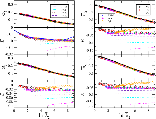
Figure 1: In the upper panel of each of the above four subfigures, $\bar{\omega}_{l}$ for $l=2$ (left top), 3 (left bottom), 4 (right top), and $5$ (right bottom) is plotted against $\ln\bar{\lambda}_{l^{\prime}}$ for $l^{\prime}=2$ case. Five kinds of realistic NSs (including AU, UU, WS, BBB2 and FPS EOSs), one QS, and the incompressible star (indicated by the black solid line) are considered (see the legend in the right-top subfigure). In the lower panel of each subfigure, the fractional deviation $E$ from the incompressible limit (the solid line in the upper panel) is shown as a function of $\ln\bar{\lambda}_{l^{\prime}}$ for $l^{\prime}=2$ case. In addition to the data of the realistic stars mentioned above, we include in the lower panel the data of polytropic stars with $\Gamma=1.8,2,2.2,2.5$ (see the legend in the upper panel of the left-top subfigure). For the diagonal case with $l=l^{\prime}$, the (blue) continuous line in the lower panel shows the fractional deviation between the scaled frequencies given respectively by the best fitting curve (9) and the incompressible limit.

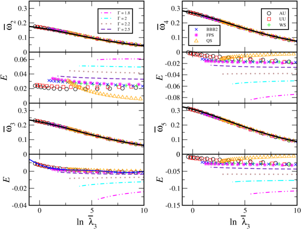
Figure 2: Similar to Fig. 1, except that the case $l^{\prime}=3$ is considered here.

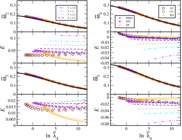
Figure 3: Similar to Fig. 1, except that the case $l^{\prime}=4$ is considered here.

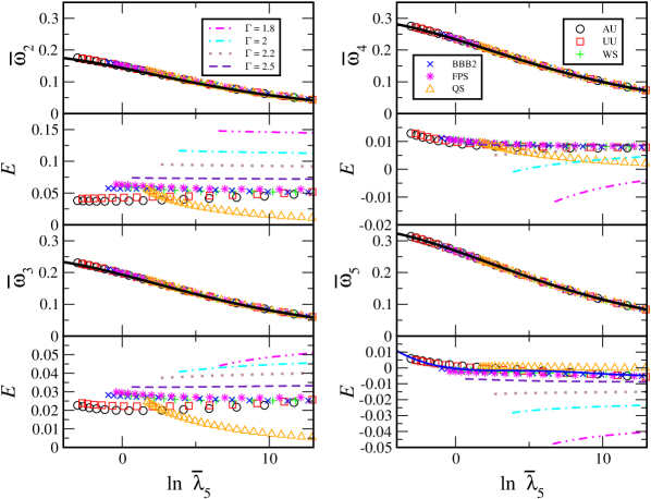
Figure 4: Similar to Fig. 1, except that the case $l^{\prime}=5$ is considered here.

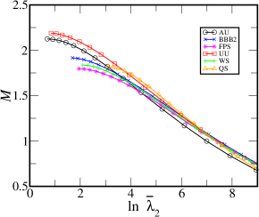
Figure 5: The masses (in $M_{\odot}$) of the realistic compact stars considered in Figs. 1-4 are shown against $\ln{\bar{\lambda}}_{2}$.

In the present paper, we adopted the convention introduced in (Damour and Nagar, 2009; Yagi, 2014) to discuss multipolar tidal deformation. We consider the $l$th order electric tidal deformability (see (Damour et al., 1992; Damour and Nagar, 2009; Yagi, 2014) for its definition), $\lambda_{l}$, with $l$ being the angular momentum index of the tidal field in consideration, as well as the dimensionless $l$th order electric tidal deformability

$$\bar{\lambda}_{l}\equiv\frac{\lambda_{l}}{M^{2l+1}},$$ (5)

which is also related to $l$th order electric tidal Love number $k_{l}$ through the relation (Damour and Nagar, 2009)

$$k_{l}\equiv\frac{(2l-1)!!}{2}{\cal C}^{2l+1}\bar{\lambda}_{l}.$$ (6)

As highlighted above, we investigate the relationship between the $l$th multipole scaled $f$-mode frequency $\bar{\omega}_{l}\equiv M{\omega}_{l}$ and the $l^{\prime}$th multipole dimensionless deformability ${\bar{\lambda}}_{l^{\prime}}$. In general, the values of $l$ and $l^{\prime}$ can be distinct. In Figs. 1-4, $\bar{\omega}_{l}$ is plotted against $\ln{\bar{\lambda}}_{l^{\prime}}$ (the upper panel), where $l=2,3,4,5$, and $l^{\prime}=2$ (Fig. 1), $l^{\prime}=3$ (Fig. 2), $l^{\prime}=4$ (Fig. 3) and $l^{\prime}=5$ (Fig. 4), for five kinds of realistic NSs (respectively constructed with AU (Wiringa et al., 1988), UU (Wiringa et al., 1988), WS (Lorenz et al., 1993; Wiringa et al., 1988), BBB2 (Baldo et al., 1997) and FPS Pandharipande and Ravenhall (1989); Lorenz et al. (1993) EOSs), one QS described by the MIT bag model (see, e.g., (Johnson, 1975; Alcock et al., 1986; Witten, 1984)), and incompressible stars. For reference, the masses of the realistic compact stars considered here are shown in Fig. 5 where $M$ (in $M_{\odot}$) is plotted against $\ln{\bar{\lambda}}_{2}$.

At first sight, all such $\bar{\omega}_{l}$ versus $\ln{\bar{\lambda}}_{l^{\prime}}$ graphs demonstrate a certain degree of EOS independence. In particular, all data points of realistic NSs and QSs nearly coalesce onto the solid line representing the data of incompressible stars. To further examine the degree of accuracy of the universal relations manifested in these curves, we use the case of incompressible stars as a reference and show the fractional deviation $E\equiv(\bar{\omega}_{l}-\bar{\omega}_{l}^{(0)})/\bar{\omega}_{l}^{(0)}$, where $\bar{\omega}_{l}^{(0)}$ is the scaled frequency of incompressible stars, in the lower panel of each of these plots. It is clearly shown that for a fixed $l^{\prime}$, $|E|$ is the smallest for the diagonal case where $l=l^{\prime}$ and, in addition, also least sensitive to EOS (including both NSs and QSs). In fact, $|E|$ is less than 0.01 in all diagonal cases considered here. Generally speaking, for the off-diagonal cases where $l\neq l^{\prime}$, the fractional deviation $E$ of QSs deviates obviously from those of NSs.

To investigate how the fractional deviation $E$ in $\bar{\omega}_{l}$ depends on the stiffness of a star, we also show in Figs. 1-4 $E$ versus $\ln\bar{\lambda}_{l^{\prime}}$ for polytropic stars with different values of relativistic adiabatic index $\Gamma\equiv[(\rho+p)/p](dp/d\rho)=1+1/N$, where $\rho$, $p$, and $N$ are energy density, pressure and the polytropic index, respectively. Save for some “atypical cases” which will be further discussed later, the diagonal $f$-Love relations again yield the smallest deviation from the incompressible limit and demonstrate the least dependence on the adiabatic index $\Gamma$. We also note that $|E|$ increases with the polytropic index $N$ and markedly grows if $N>1$, especially for dense stars close to the maximum mass limit (i.e., stars with small scaled tidal deformability). As a rule of thumb, general relativistical effects could apparently soften the stiffness of matter and lead to a smaller effective value of the adiabatic index (see, e.g., (Chandrasekhar, 1964, 1965) and Chap. 6 of (Shapiro and Teukolsky, 1983) for a heuristic explanation for the decrease in the effective adiabatic index due to gravitational effect). For example, NSs with adiabatic index $\Gamma>$ 2 still become unstable towards the high compactness end as a result of the decrease in the effective value of $\Gamma$. Similarly, the reduction of the effective value of $\Gamma$ also explains the increase in $E$ towards the maximum mass limit observed in Figs. 1-4. The above-mentioned observations clearly indicate that the stiffness of nuclear EOS is a crucial factor affecting the $f$-Love relation discovered here.

Moreover, some interesting behaviors of $E$ can be observed from the graphs shown in Figs. 1-4. For all diagonal cases, $E$ is negative (except near the maximum mass limit in Fig. 1) and its magnitude decreases with the stiffness (or $\Gamma$) of the EOS. For nondiagonal cases showing $E$ in the plots of $\bar{\omega}_{l}$ versus $\ln{\bar{\lambda}}_{l^{\prime}}$, if $l>l^{\prime}$, the above-mentioned behavior of $E$ remains unchanged. In fact, $|E|$ also increases with $l$ for a fixed $l^{\prime}$. However, the situation for cases with $l<l^{\prime}$ becomes more complicated. For the diagrams of $E$ with $(l,l^{\prime})=(2,3),(2,4),(2,5),(3,5)$, $E$ becomes positive although its magnitude still decreases with increasing stiffness (or increasing $\Gamma$). On the other hand, for the “atypical cases” with $(l,l^{\prime})=(3,4),(4,5)$ there are some crossings between lines representing EOSs of different stiffness and the sign of $E$ is not uniquely defined. Thus, the magnitude of $E$ is no longer a good indicator for the stiffness of EOS.

Based on these observations, we figure out a phenomenological method, whose analytical basis will be provided in Sec. IV, to explain the above-mentioned behavior of $E$. Schematically we expand $E$ in power series of $N$,

$$E(\ln{\bar{\lambda}}_{l^{\prime}};l,l^{\prime};N)=E_{1}(l,l^{\prime})N+E_{2}(l,l^{\prime})N^{2},$$ (7)

where the coefficients $E_{1}(l,l^{\prime})$ and $E_{2}(l,l^{\prime})$ in general could also depend on ${\bar{\lambda}}_{l^{\prime}}$, and only terms up to $N^{2}$ are kept in the expansion. As shown in Figs. 1-4, as long as $N<1$, $E$ is insensitive to changes in $N$ for the diagonal case. Hence, it is reasonable to assume that if $l=l^{\prime}$, $E_{1}$ vanishes and is proportional to $l-l^{\prime}$ (or any of its positive powers). Without loss of generality, we rewrite (7) as

$$E(\ln{\bar{\lambda}}_{l^{\prime}};l,l^{\prime};N)=-\alpha(l-l^{\prime})N-\beta N^{2},$$ (8)

where $\alpha$ and $\beta$ (both are dependent on $l,l^{\prime}$) are assumed to be positive constants in order to explain the numerical data shown in the figures. Therefore, for the diagonal cases with $l=l^{\prime}$, $E=-\beta N^{2}<0$ and $|E|$ increases with $N$. This successfully captures the trend observed in Figs. 1-4. In fact, we have verified this point (within the accuracy of available numerical data) in Figs. 1-4 in the Newtonian limit (see also Table 3).

On the other hand, for off-diagonal cases with $l>l^{\prime}$, it follows from (8) that $E$ is still negative and $|E|$ also increases with $N$. Complication arises for off-diagonal cases with $l<l^{\prime}$. Several situations could be possible. Two of them are: (i) If either $N$ is small or $|l-l^{\prime}|$ is large, then the first-order term dominates the second-order term. Consequently, $E$ is positive and increases with $N$ [see the diagrams of $E$ with $(l,l^{\prime})=(2,3),(2,4),(2,5),(3,5)$]. (ii) If the first-order and the second-order terms are of similar magnitudes, they could partly cancel each other out. Hence, $E$ is not of a definite sign and its magnitude may be rather small due to the cancellation of these two terms. Such is the explanation for the atypical cases mentioned above [cases with $(l,l^{\prime})=(3,4),(4,5)$]. Hence, in these atypical cases the magnitude of the deviation could not used as a direct measure of the stiffness of nuclear matter.

However, (8) has to be properly modified in order to account for relativistic effects. As can be observed from the diagonal cases in Figs. 1-4, for a fixed EOS $|E|$ usually increases towards the maximum mass limit, which could be understood as the consequence of the general relativistical softening effect mentioned above. Therefore, the polytropic index $N$ used in (8) should be replaced by its modified value, which is expected to be larger than the original value. Such replacement can qualitatively explain the increase in $|E|$ observed for dense stars. Empirically, we find that the modified polytropic index $N$ increases by an amount of the order of the compactness of the star, which is in agreement with the post-Newtonian analysis carried out in (Chandrasekhar, 1964, 1965). On the other hand, a subtlety can also be observed from these figures especially for stiff stars in the small $\bar{\lambda}$ regime (i.e., dense stars). It seems that an extra anomalous (positive) contribution emerges in the right-hand side of (7). For example, in the diagonal case of Fig. 1, both the curves with $\Gamma=2.5,2.2$ cross zero in the small $\bar{\lambda}$ regime. We expect the magnitude of this extra term, which is more important for stiff stars, grows with compactness and leads to this anomalous behavior. However, the effect of this anomalous term is quite small and we cannot extract its quantitative dependence from our data.

To sum up the above observations, we find that both realistic NSs and QSs obey the $f$-Love universal relation as shown in Figs. 1-4. Such universal behavior, which is shown to be insensitive to changes in polytropic index $N$ as long as $N$ is less than unity (see Figs. 1-4), is attributable to the fact that realistic NSs far from the theoretical minimum mass limit are made of stiff nuclear matter with $N<1$. On the other hand, for QSs obeying the simple MIT bag model (see, e.g., (Chodos et al., 1974; Glendenning, 1997; Weber, 1999)), it is straightforward to show that $N=\rho/(4B)-1$, where $B$ is the bag constant. Unless for QSs with central density much higher than the bag constant, $N$ is also less than unity. In fact, $N$ is almost zero for low mass QSs. Hence, QSs also reveal similar $f$-Love universal behavior.

Lastly, we note that the diagonal $f$-Love universal relation can be represented by the following empirical formula

$$\bar{\omega}_{l}=\bar{a}_{0}+\bar{a}_{1}x+\bar{a}_{2}x^{2}+\bar{a}_{3}x^{3}+\bar{a}_{4}x^{4}~{},$$ (9)

where $x=\ln\bar{\lambda}_{l}$. The coefficients $\bar{a}_{0}$, $\bar{a}_{1}$, $\bar{a}_{2}$, $\bar{a}_{3}$ and $\bar{a}_{4}$ for $l=2,3,4,5$ obtained from the best fit to the data of the realistic stars considered in Figs. 1-4 are tabulated in Table 1. For reference, the fractional deviation between the values of $\bar{\omega}_{l}$ given, respectively, by (9) and the incompressible limit is also shown in the lower panel of each subfigure (the blue continuous line) of Figs. 1-4. It can be clearly seen that the fractional deviation is usually less than 0.01. This again supports our claim that the $f$-Love universal relation of realistic stars follows that of incompressible stars.

	$l=2$	$l=3$	$l=4$	$l=5$
$\bar{a}_{0}$	$1.820\times 10^{-1}$	$~{}~{}2.245\times 10^{-1}$	$~{}~{}2.501\times 10^{-1}$	$~{}~{}2.681\times 10^{-1}$
$\bar{a}_{1}$	$-6.836\times 10^{-3}$	$-1.500\times 10^{-2}$	$-1.646\times 10^{-2}$	$-1.638\times 10^{-2}$
$\bar{a}_{2}$	$-4.196\times 10^{-3}$	$-1.412\times 10^{-3}$	$-5.897\times 10^{-4}$	$-2.497\times 10^{-4}$
$\bar{a}_{3}$	$~{}~{}5.215\times 10^{-4}$	$~{}~{}1.832\times 10^{-4}$	$~{}~{}8.695\times 10^{-5}$	$~{}~{}4.712\times 10^{-5}$
$\bar{a}_{4}$	$-1.857\times 10^{-5}$	$-5.561\times 10^{-6}$	$-2.368\times 10^{-6}$	$-1.166\times 10^{-6}$

Table 1: The coefficients $\bar{a}_{0}$, $\bar{a}_{1}$, $\bar{a}_{2}$, $\bar{a}_{3}$ and $\bar{a}_{4}$ in the empirical formula (9) are tabulated for $l=2,3,4,5$.

IV Newtonian analysis

IV.1 Generalized Tolman model

In the previous section, we have shown that the diagonal $f$-Love relation is particularly insensitive to variations in EOS and the behavior of realistic stars and polytropic stars tends to that of incompressible stars as long as these stars are sufficiently stiff. On the other hand, the off-diagonal counterpart displays more sensitive dependence on stiffness. To provide these observations a proper theoretical basis, at least in the Newtonian limit, we consider a model compact star, referred to as the generalized Tolman model (GTM) in the present paper, whose density distribution $\rho(r)$ depends on the radial coordinate $r$ as follows:

$$\rho(r)=\rho_{0}f(x,\delta),$$ (10)

with $\rho_{0}$ being the central density, $x\equiv r/R$, $0\leq\delta\leq 1$ and

$$f(x,\delta)\equiv 1-\delta x^{2}~{}.$$ (11)

Here $\delta$ is a parameter determining the stiffness of the EOS of the star, which can be quantitatively measured by a position-dependent effective polytropic index $N_{\rm e}(\delta;x)$, where

$$\left[N_{\rm e}(\delta;x)\right]^{-1}\equiv\frac{\rho}{p}\frac{dp}{d\rho}-1$$ (12)

$$= \frac{(1-\delta x^{2})^{2}(5-3\delta x^{2})}{\delta[5(1-x^{2})-4\delta(1-x^{4})+\delta^{2}(1-x^{6})]}-1.~{}~{}~{}~{}~{}$$

The GTM (11) reduces to nearly incompressible and Tolman VII model stars in the limits $\delta\ll 1$ and $\delta\approx 1$, respectively (Seidov and Kuzakhmedov, 1978; Seidov, 2004; Lattimer and Prakash, 2001; Lake, 2003; Postnikov et al., 2010). For $\delta\ll 1$, it can be shown that $N_{\rm e}\approx\delta$ for $x\leq\delta$. In fact, near the center of the star, (11) closely resembles the density distribution of a polytropic star with polytropic index $N=\delta$, whose density is, to leading order in $N$, given by (Seidov and Kuzakhmedov, 1978; Seidov, 2004)

$$\rho(r)=\rho_{0}[1+N\ln(1-x^{2})].$$ (13)

Therefore, this model can nicely approximate nearly incompressible stars in the small-$\delta$ limit. On the other hand, if $\delta$ is equal to unity, the model obviously reduces to the standard Tolman VII model, which has been shown to be a good approximation of realistic NSs (Lattimer and Prakash, 2001; Lake, 2003; Postnikov et al., 2010). This is the reason why the model (11) is coined here as the generalized Tolman model. Besides, unless $\delta=1$, there is a density discontinuity developed at the stellar surface, which prevails in bare QSs (see, e.g., (Glendenning, 1997; Weber, 1999) and references therein). Hence, the GTM is also capable of reproducing such typical behavior of QSs.

Furthermore, we have also verified that the effective polytropic index $N_{\rm e}$ in (12) is always less than or equal to unity for all physical choices of $\delta$ and $x$. For example, for the case with $\delta=1$ (i.e., the standard Tolman VII model), $N_{\rm e}=1$ at the stellar surface and decreases monotonically to $2/3$ at the center $x=0$ (Lau, 2009). For $\delta<1$, the corresponding value of $N_{\rm e}$ is also less than unity everywhere inside the star. Hence, we expect that GTM is a valid model to emulate sufficiently stiff NSs and QSs whose effective polytropic index is less than unity. In the following discussion, we shall make use of the simplicity and manageability of GTM to study the underlying physical mechanism of the universal $f$-Love relation discovered here. First, two universal formulas respectively connecting the $f$-mode frequency and the tidal deformability to mass moments of suitable orders are derived. Each of these analytic formulas constitutes the generalization of $f$-$I$ and $I$-Love relations to multipolar cases. The mass moment is then eliminated from these two formulas and hence the $f$-Love relation in the Newtonian limit is obtained.

IV.2 $f$-$I$ relation

It can be shown from the variational method proposed by Chandrasekhar Chandrasekhar (1963) that the frequency of the $l$th multipole $f$-mode oscillation, $\omega_{l0}\equiv\omega_{l}$ (the subscript “$0$” stands for $f$ mode and is suppressed unless otherwise stated), of compact stars is approximately given by (Chan, 2012)

$$\omega_{l}^{2}=\frac{2l(l-1)(2l-1)}{2l+1}\frac{\int_{0}^{R}pr^{2l-2}{d}r}{\int_{0}^{R}\rho r^{2l}{d}r}.$$ (14)

Here $p$ is the pressure at radius $r$, which can be obtained from the hydrodynamic equilibrium condition (see, e.g., (Cox, 1980)). In (14) the quasiincompressible fluid approximation that the Lagrangian displacement $\bm{\xi}_{l0}\propto{\bm{\nabla}}(r^{l}Y_{lm})$, where $Y_{lm}$ is the spherical harmonic function, has been made. Such approximation stems from the observation that in $f$-mode oscillations of stiff stars the Lagrangian change in density is negligible except perhaps near the stellar surface. As shown in Table 2, the accuracy of (14) is excellent as long as the star concerned is stiff. In particular, for incompressible stars (i.e., GTM stars with $\delta=0$) the approximation turns out to be exact and for QSs the percentage errors in $\omega_{l}^{2}$ ($l=2$ in the table) are less than $4\times 10^{-3}\%$. On the other hand, for polytropic stars with polytropic index $N$ less than unity and a realistic star (with FPS EOS) the percentage error is still less than $1.6\%$. However, the accuracy of the approximation deteriorates with increasing value of the polytropic index. As the polytropic index for typical NSs whose mass is greater than $1M_{\odot}$ is less than 1, the quasiincompressible approximation is justified.

Table 2: $R^{3}\omega_{2}^{2}/(GM)$, where $\omega_{2}$ is the quadrupole $f$-mode oscillation frequency, is shown for various stars, including polytropic stars with different polytropic indices $N$, two GTM stars ($\delta=0,1$), a FPS NS (with central density $10^{15}\,\mathrm{g}\,\mathrm{cm}^{-3}$), and two QSs (${\cal C}=0.0811,0.1719$) with $B^{1/4}=154.5\,{\rm MeV}$. The four columns indicate the EOS of the star, the exact values of $R^{3}\omega_{2}^{2}/M$, the corresponding approximate values obtained from (14) and the associated percentage errors, respectively.

EOS	Exact	(14)	Error
Poly($N=3.0$)	5.880	10.60	80.3%
Poly($N=2.5)$	4.311	5.722	32.7%
Poly($N=2.0$)	3.026	3.431	13.4%
Poly($N=1.7)$	2.441	2.635	7.9%
Poly($N=1.5)$	2.119	2.221	4.8%
Poly($N=1.0)$	1.505	1.529	1.6%
Poly($N=0.8)$	1.320	1.331	0.8%
Poly($N=0.6)$	1.160	1.164	0.3%
GTM($\delta=0$)	0.800	0.000	0.0%
GTM($\delta=1$)	1.324	1.333	0.74%
FPS	1.397	1.402	0.4%
QS(${\cal C}=0.0811)$	0.8177	0.8177	$4.4\times 10^{-4}\%$
QS(${\cal C}=0.1719)$	0.8403	0.8404	$3.9\times 10^{-3}\%$

For GTM, whose the density is given by (10), $\omega_{l}^{2}$ acquires the following explicit form:

$$\omega_{l}^{2}=\frac{8\pi\rho_{0}Gl(l-1)}{3}\frac{\int_{0}^{1}x^{2l}f(x,\delta)f(x,3\delta/5){d}x}{\hat{f}\left(\frac{2l+1}{2l+3}\delta\right)},$$ (15)

where $\hat{f}(y)=f(x=1,y)$. As expected, $\omega_{l}^{2}$ is proportional to $\rho_{0}$. However, in general, the proportional constant is dependent on the value of $\delta$, i.e., the EOS.

The GTM is characterized by two physical parameters, namely the central density $\rho_{0}$ and the stellar radius $R$. Both the $f$-mode oscillation frequency in (15) and the tidal deformability (to be discussed later) are dependent on them. However, these two parameters are also expressible in terms of any two of the mass moments:

$$I_{n}\equiv\int_{0}^{R}\rho(r)r^{2+n}{d}r=\frac{\rho_{0}R^{3+n}}{n+3}\hat{f}\left(\frac{n+3}{n+5}\delta\right),$$ (16)

where $n=0,1,2,\cdots$, and, for simplicity, the solid angle $4\pi$ is omitted in the definition of $I_{n}$, as follows:

$$\rho_{0} = \frac{(n+3)^{3/n}I_{0}^{1+3/n}\left[\hat{f}\left(\frac{n+3}{n+5}\delta\right)\right]^{3/n}}{3^{1+3/n}I_{n}^{3/n}\left[\hat{f}\left(\frac{3\delta}{5}\right)\right]^{1+3/n}},$$ (17)

$$R^{n} = \frac{(n+3)I_{n}\hat{f}\left(\frac{3\delta}{5}\right)}{3I_{0}\hat{f}\left(\frac{n+3}{n+5}\delta\right)}.$$ (18)

Therefore, the $f$-mode oscillation frequency and the tidal deformability can be determined from $M=4\pi I_{0}$ and $I_{n}$ ($n=1,2,3,\cdots$) and we have the freedom to choose the value of $n$.

Substituting the above expression for $\rho_{0}$ into (15), we can express $\omega^{2}_{l}$ in terms of simple algebraic functions of $\delta$. In particular, apart from a trivial $\delta$-independent proportional constant, we find that to first order in $\delta$,

$$\omega_{l}^{2}\propto\left(\frac{M^{n+3}}{I_{n}^{3}}\right)^{1/n}\left\{1+\frac{6\delta(n+2-2l)}{5(n+5)(2l+3)}\right\},$$ (19)

and, most interestingly, the coefficient of $\delta$ in the above expansion vanishes if $n=2l-2$. Besides, it can also be shown that $\delta=1$ is always a stationary point of $\omega_{l}^{2}$ irrespective of the values of $l$ and $n$. Therefore we expect that the dependence of $\omega_{l}^{2}$ on $\delta$ is relatively weak if $n=2l-2$. Hence, we arrive at the universal “diagonal” multipolar $f$-I relation

$$\bar{\omega}_{l}^{2}=A_{l}(\delta)\left(\frac{M^{2l-1}}{I_{2l-2}}\right)^{\frac{3}{2l-2}},$$ (20)

where the coefficient $A_{l}(\delta)$ is to first order independent of $\delta$, and, in particular,

$$A_{l}(\delta=0)\equiv A_{l}^{(0)}=\frac{2l(l-1)}{(2l+1)^{\frac{2l+1}{2l-2}}}\left(\frac{3}{4\pi}\right)^{\frac{3}{2l-2}}.$$ (21)

It is interesting to note that to first order in $\delta$, $(\bar{\omega}_{2})^{2}=A_{2}^{(0)}(M^{3}/I_{2})^{3/2}\propto\eta^{3}$, which can be considered as the Newtonian extension of the quadrupole $f$-$I$ relation (1). In Fig. 6 (top panel), we show $\Delta_{a}\equiv A_{l}(\delta)/A_{l}^{(0)}-1$ as a function of $\delta$. It is obvious that $\Delta_{a}$ is limited to a few percent for all physical values of $\delta$. Thus, the validity of the $f$-$I$ relation is established.

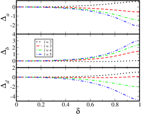
Figure 6: Plots of $\Delta_{a}$ (top), $\Delta_{b}$ (middle) and $\Delta_{d}$ (bottom) versus $\delta$ for GTM with $l=2,3,4$ and $5$. In all cases, $\Delta$’s are measured in percent.

IV.3 $I$-Love relation

Similarly, we can evaluate the tidal deformability of GTM as follows. In the Newtonian limit, the metric coefficient $H_{l}$ satisfies (Damour and Nagar, 2009; Yagi and Yunes, 2013a; Yagi, 2014)

$$\frac{d^{2}H_{l}}{dr^{2}}+\frac{2}{r}\frac{dH_{l}}{dr}-\frac{l(l+1)}{r^{2}}H_{l}=-4\pi\rho\frac{d\rho}{dP}H_{l},$$ (22)

which is essentially the Poisson equation in Newtonian gravity with its right-hand side measuring the Eulerian change in density due to tidal deformation, and the right-hand side of the above equation vanishes identically outside the star. Once $H_{l}$ is found, $\bar{\lambda}_{l}$ is given by (Damour and Nagar, 2009)

$$\bar{\lambda}_{l}=\frac{1}{(2l-1)!!\,{\cal C}^{2l+1}}\frac{l-y_{l}}{l+1+y_{l}},$$ (23)

where

$$y_{l} \equiv \left(\frac{r}{H_{l}}\frac{dH_{l}}{dr}\right)_{r=R^{+}}$$ (24)

$$= \left(\frac{r}{H_{l}}\frac{dH_{l}}{dr}-\frac{4\pi R^{3}\rho}{M}\right)_{r=R^{-}}.$$

For the GTM considered above, Eq. (22) can be exactly solved:

$$H_{l}(r)=r^{l}\,_{2}F_{1}\left(a,b;d;\zeta\right),$$ (25)

where ${}_{2}F_{1}(a,b;d;\zeta)$ is the standard hypergeometric function, with

$$a = \frac{1+2l-\Xi}{4},$$ (26)

$$b = \frac{1+2l+\Xi}{4},$$ (27)

$$\Xi = \sqrt{4l^{2}+4l+41},$$ (28)

$$d = \frac{3}{2}+l,$$ (29)

$$\zeta = \frac{3\delta r^{2}}{5R^{2}},$$ (30)

and, as usual, regularity of $H_{l}$ at the origin is assumed. Hence, we can analytically find $y_{l}$:

$$y_{l}=l-\frac{6\delta\,_{2}F_{1}\left(a_{1},b_{1};d_{1};\frac{3\delta}{5}\right)}{(2l+3)\,_{2}F_{1}\left(a,b;d;\frac{3\delta}{5}\right)}-\frac{15(1-\delta)}{5-3\delta},$$ (31)

where $a_{1}=a+1$, $b_{1}=b+1$, and $d_{1}=d+1$. Expressing $R$ in terms of $I_{n}$, we find that to first order in $\delta$,

$$(2l-1)!!M^{2l+1}\bar{\lambda}_{l}\left[\frac{(n+3)I_{n}}{3I_{0}}\right]^{-\frac{2l+1}{n}}$$ (32)

$$= \left[\frac{3}{2l-2}+\frac{3(2l+1)(2l-2-n)\delta}{5(l-1)(2l+3)(n+5)}\right].$$

If $n=2l-2$, to first order in $\delta$, $\bar{\lambda}_{l}$ is simply proportional to $(I_{n}/M)^{(2l+1)/n}$ with a $\delta$-independent proportional constant. Such a case also holds if $1-\delta\ll 1$ for all values of $n$. The situation is similar to the analysis developed previously for the $f$-$I$ relation. As a consequence, the universal “diagonal” multipolar $I$-Love formula can be expressed as

$$\bar{\lambda}_{l}=B_{l}\left(\frac{I_{2l-2}}{M^{2l-1}}\right)^{\frac{2l+1}{2l-2}},$$ (33)

where $B_{l}(\delta)$ depends only weakly on $\delta$, with $(dB_{l}/d\delta)_{\delta=0}=0$ and

$$B_{l}(\delta=0)\equiv B_{l}^{(0)}$$ (34)

$$= \frac{3}{2(l-1)[(2l-1)!!]}\left[\frac{4\pi(2l+1)}{3}\right]^{\frac{2l+1}{2l-2}}.$$

For $l=2$, Eq. (33) leads to $\bar{\lambda}_{2}=B_{2}^{(0)}(I_{2}/M^{3})^{5/2}$ to first order in $\delta$, which is in agreement with the result obtained in (Yagi and Yunes, 2013a). Figure 6 (middle panel) plots $\Delta_{b}\equiv B_{l}(\delta)/B_{l}^{(0)}-1$ against $\delta$ for $l=2,3,4,5$. Again $\Delta_{b}$ is at most a few percent for $0\leq\delta\leq 1$, which guarantees the accuracy of the multipolar $I$-Love relation. However, it is obvious that EOS dependence of such diagonal relations grows gradually with increasing value of $l$.

IV.4 $f$-Love relation

Eliminating the mass moment $I_{2l-2}$ from (20) and (33), we arrive at the Newtonian form of the diagonal multipolar $f$-Love universal relation:

$$\bar{\omega}_{l}^{2}\bar{\lambda}_{l}^{\frac{3}{2l+1}}=D_{l}(\delta),$$ (35)

where $D_{l}(\delta)$ is an EOS-insensitive function with $(dD_{l}/d\delta)_{\delta=0}=0$ and for $\delta=0$:

$$D_{l}(\delta=0)\equiv D_{l}^{(0)}$$ (36)

$$= \frac{2l(l-1)}{2l+1}\left[\frac{3}{2(l-1)(2l-1)!!}\right]^{\frac{3}{2l+1}}.$$

The plot of $\Delta_{d}\equiv D_{l}(\delta)/D_{l}^{(0)}-1$ versus $\delta$ in Fig. 6 (bottom panel) firmly corroborates the EOS-insensitive multipolar $f$-Love relation derived above. Besides, the universal Newtonian relation in (35) is verified in Fig. 7 where $2\ln\bar{\omega}_{l}$ is plotted against $[3/(2l+1)]\ln\bar{\lambda}_{l}$ with $l=2,3,4,5$ for incompressible stars (i.e., $\delta=0$). In the Newtonian limit, all curves tend to straight lines with the same slope but slightly different intercepts, which agree with the value given by (36).

Similarly, the off-diagonal $f$-Love relation can also be obtained and is shown below for purpose of comparison:

$$\bar{\omega_{l}}^{2}\bar{\lambda}_{l^{\prime}}^{\frac{3}{2l^{\prime}+1}}=D_{ll^{\prime}}^{(0)}\left[1-\frac{12(l-l^{\prime})\delta}{5(2l^{\prime}+3)(2l+3)}+...\right],$$ (37)

where

$$D_{ll^{\prime}}^{(0)}=\frac{2l(l-1)}{2l+1}\left[\frac{3}{2(l^{\prime}-1)(2l^{\prime}-1)!!}\right]^{\frac{3}{2l^{\prime}+1}}.$$ (38)

In general, for $l\neq l^{\prime}$, the $\delta$-term in the right-hand side of (37) does not vanish, implying that the off-diagonal universal relation would demonstrate more obvious EOS dependence. This clearly explains our findings in the previous section and further supports the phenomenological model proposed in (7) and (8).

Moreover, we have evaluated $\bar{\omega}_{l}$, $\bar{\lambda}_{l}$ and $I_{2l-2}$ ($l=2,3,4,5$) for polytropic stars with different polytropic indices and evaluated $A_{l}$, $B_{l}$ and $D_{l}$ from (20), (33) and (35), respectively. In Table 3 we compare these values with their incompressible counterparts to find $\Delta_{a}$, $\Delta_{b}$ and $\Delta_{c}$. Again we find that the deviations are small as long as $N\leq 1$ and indeed proportional to $N^{2}$ (or higher) within the accuracy our numerical data. In fact, for the $l=2$ case all $\Delta$’s approximately behave as $N^{4}$, while in other cases they grow gradually with $l$.

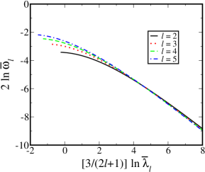
Figure 7: Plot of $2\ln\bar{\omega}_{l}$ against $[3/(2l+1)]\ln\bar{\lambda}_{l}$ for incompressible stars with $l=2,3,4$ and $5$.

$N$	$l=2$	$l=3$	$l=4$	$l=5$
$5/3$	$(-4.6,3.3,-2.7)$	$(-11,9.9,-7.6)$	$(-15,14,-11)$	$(-16,16,-13)$
$1.25$	$(-1.5,1.1,-0.93)$	$(-5.4,4.7,-3.5)$	$(-7.6,6.9,-5.5)$	$(-8.8,8.4,-6.8)$
$1$	$(-0.61,0.34,-0.4)$	$(-3.1,2.7,-2.0)$	$(-4.6,4.1,-3.3)$	$(-5.5,5.1,-4.2)$
$5/6$	$(-0.24,0.11,-0.17)$	$(-2.0,1.7,-1.2)$	$(-3.0,2.8,-2.1)$	$(-3.7,3.5,-2.8)$
$2/3$	$(-0.011,-0.022,-0.024)$	$(-1.1,1.0,-0.68)$	$(-1.8,1.8,-1.3)$	$(-2.3,2.2,-1.7)$

Table 3: In each entry the triplet ($\Delta_{a}\times 100\%$, $\Delta_{b}\times 100\%$, $\Delta_{c}\times 100\%$) is shown for various values of the polytropic index $N$ and $l=2,3,4,5$.

V $f$-$I$-Love relation

Instead of eliminating the mass moment $I_{2l-2}$, we can remove mass $M$ from (20) and (33) to obtain an equation linking ${\lambda_{l}}$, ${\omega}_{l}^{2}$ and ${I_{2l-2}}$ together:

$${\lambda_{l}}{\omega}_{l}^{2}=\frac{4\pi l}{(2l-1)!!}{I_{2l-2}}.$$ (39)

This equation, coined as the $f$-$I$-Love relation in the present paper, indeed connects three physical quantities, namely the $f$-mode frequency $\omega_{l}$, tidal deformation $\lambda_{l}$ and the mass moment $I_{2l-2}$ together. It is noteworthy that each of them carries proper dimensions and the mass $M$ completely disappears in (39). Comparing the $f$-$I$-Love relation (39) with the $f$-Love relation (35), the mass moment $I_{2l-2}$ in the former actually plays the role of $M$ in the latter.

We have derived the $f$-$I$-Love relation (39) from the GTM assumed above. However, to show the robustness of (39), in the following we apply the linear response theory (Green’s function method) to quasiincompressible stars to develop an independent proof for it.

In Newtonian theory, the steady state response of a star to an external time-dependent potential $U({\bf r})\exp(-i\omega t)$ of frequency $\omega$ can be obtained from the Green’s function method to be detailed as follows (Chandrasekhar, 1963; Press and Teukolsky, 1977). First of all, the normal modes of a star are defined by the solutions to the eigenvalue equation:

$$({\cal L}-\rho_{\rm e}\omega^{2}_{ln})\bm{\xi}_{ln}=0,$$ (40)

where $\rho_{\rm e}(r)$ is the density distribution of the equilibrium state and $\omega_{ln}$ and $\bm{\xi}_{ln}$ are the eigenfrequency and the Lagrangian displacement of the $n$th ($n=0,1,2,\ldots$) oscillation mode carrying angular momentum $l=0,1,2,3,\ldots$. The $l=0$ case corresponds to radial oscillation, $l=1$ case usually represents translational motion, and for $l\geq 2$ cases the star undergoes nonradial oscillations. Unless otherwise stated explicitly, the $z$ component of angular momentum, $m$, is suppressed in our equations. We adopt the convention where $\omega_{l0}<\omega_{l1}<\omega_{l2}\cdots$. For barotropic stars, which is always assumed in our analysis, the 0th mode is the $f$ mode. Besides, $-{\cal L}\bm{\xi}$ in general represents the net internal restoring force (including pressure force and the gravitational force due to the star itself) acting on a fluid element, which can be obtained from the Lagrangian displacement $\bm{\xi}$. The explicit form of ${\cal L}$ can be found in (Chandrasekhar, 1963). Most importantly, ${\cal L}$ is a Hermitian operator guaranteeing the orthogonality relation of $\bm{\xi}_{ln}$ (Chandrasekhar, 1963):

$$\langle\bm{\xi}_{lj}^{*}|\bm{\xi}_{l^{\prime}n}\rangle\equiv\int_{V}\rho_{\rm e}\bm{\xi}_{lj}^{*}\cdot\bm{\xi}_{l^{\prime}n}d^{3}r=\delta_{ll^{\prime}}\delta_{jn},$$ (41)

where $V$ here denotes the volume of the star and the displacement fields are properly normalized to accord with (41).

In the presence of an external time-dependent gravitational potential $U({\bf r})\exp(-i\omega t)$, the steady state linear response of the Lagrangian displacement $\bm{\xi}$ is given by solution of the inhomogeneous equation

$$({\cal L}-\rho\omega^{2})\bm{\xi}=-\rho_{\rm e}{\bm{\nabla}}U.$$ (42)

The right-hand side of the above equation is actually the external gravitational force exerted on the star. Expanding $\bm{\xi}$ in terms of the complete set of $\bm{\xi}_{ln}$ and using (40)-(42), we find that

$$\bm{\xi}=\sum_{l,n}\frac{\langle\bm{\xi}_{ln}|{\bm{\nabla}}U\rangle\bm{\xi}_{ln}}{\omega^{2}-\omega_{ln}^{2}}=\sum_{l,n}B_{ln}\bm{\xi}_{ln}.$$ (43)

In particular, if the external potential is a time-independent tidal potential in the $l$th ($l\geq 2$) multipolar sector, namely $U_{\rm e}=r^{l}Y_{lm}(\theta,\phi)$, where $Y_{lm}(\theta,\phi)$ is the standard spherical harmonics of angles $\theta$ and $\phi$, a corresponding multipole moment defined by

$$Q_{l}=\frac{4\pi}{2l+1}\int_{V}r^{l}\delta\rho Y_{lm}^{*}(\theta,\phi)d^{3}r$$ (44)

with $\delta\rho(\bm{r})$ being the Eulerian change in density, is induced. The induced multipole moment in turn sets an additional potential $U_{\rm p}=Q_{l}Y_{lm}(\theta,\phi)/r^{l+1}$ outside the star.

In the linear response regime $\delta\rho(\bm{r})=-{\bm{\nabla}}\cdot(\rho_{\rm e}\bm{\xi})$. The expansion in (43) then readily leads to

$$Q_{l} = \frac{4\pi}{2l+1}\sum_{l^{\prime},n}B_{l^{\prime}n}\langle{\bm{\nabla}}(r^{l}Y_{lm})|\bm{\xi}_{l^{\prime}n}\rangle$$ (45)

$$= \frac{-4\pi}{2l+1}\sum_{l^{\prime},n}\frac{|\langle{\bm{\nabla}}(r^{l}Y_{lm})|\bm{\xi}_{l^{\prime}n}\rangle|^{2}}{\omega_{l^{\prime}n}^{2}}$$

So far the calculation has been exact up to the leading order of the perturbing potential. For $f$-mode oscillations of quasiincompressible stars, the Lagrangian change in the density vanishes and hence ${\bm{\nabla}}\cdot\bm{\xi}_{l0}=0$. Taking into consideration the fact that $\bm{\xi}$ is derivable from a scalar potential (see, e.g., (Cox, 1980)), we arrive at the approximate formula $\bm{\xi}_{l0}={\bm{\nabla}}(r^{l}Y_{lm})/\langle{\bm{\nabla}}(r^{l}Y_{lm})|{\bm{\nabla}}(r^{l}Y_{lm})\rangle^{1/2}$. We note that such approximation has been put forward by Chandrasekhar Chandrasekhar (1963) as the trial input of a variational principle, which is used in Sec. III to evaluate $f$-mode oscillation frequencies. By orthogonality of the normal modes, only the $f$ mode with the same angular momentum index $l$ has to be included in the sum in (45), and after integrating by parts, we show that

$$Q_{l}\omega_{l0}^{2}=-4\pi lI_{2l-2}.$$ (46)

By virtue of (6), (46) and the definition of tidal Love number (Damour and Nagar, 2009; Yagi, 2014),

$$k_{l}=-\frac{Q_{l}}{2R^{2l+1}}=-\left(\frac{U_{\rm p}}{2U_{\rm e}}\right)_{r=R},$$ (47)

the general $f$-$I$-Love relation involving three dimensionless quantities $M\omega_{l0}\equiv\bar{\omega}_{l}$, $I_{2l-2}/M^{2l-1}$ and $\bar{\lambda_{l}}$

$$\bar{\lambda_{l}}\bar{\omega}_{l}^{2}=\frac{4\pi l}{(2l-1)!!}\left(\frac{I_{2l-2}}{M^{2l-1}}\right)$$ (48)

is established, which holds for sufficiently stiff stars and $l=2,3,4,\ldots$.

It is remarkable that (39) and (48) are in fact equivalent to each other. While the former is a consequence of $f$-$I$ and $I$-Love relations, the latter is derived directly from the Green’s function method. Given the $f$-$I$-Love relation (48) obtained from the linear response theory, the two seemingly independent $f$-$I$ and $I$-Love relations are in fact the consequence of each other for quasiincompressible stars characterized by stiff EOSs. Hence, the interrelationship between the $f$-$I$ and $I$-Love relations is clearly shown from the $f$-$I$-Love relation.

VI Conclusion and discussion

Although the $f$-$I$ relation and the $I$-Love-$Q$ relations have recently been discovered in the quadrupolar sector and various potential applications of them have been proposed (Lau et al., 2010; Yagi and Yunes, 2013a; Yagi and Yunes, 2013b), the reasons for the validity of these two relations and their interrelationship are not yet fully understood. Yagi and Yunes Yagi and Yunes (2013a); Yagi and Yunes (2013b) suggested two possible reasons for the $I$-Love-$Q$ relations: (i) the relations are most sensitive to the stellar matter in an outer layer between $70\%$ and $90\%$ of the radius of a NS and the EOS there is quite unified; and (ii) the internal stellar structure of NSs is gradually effaced as the black-hole limit is approached and hence NSs reveal similar behavior. On the other hand, more recently Yagi et al. Yagi et al. (2014) found that the $I$-Love-$Q$ relations are actually dominated by the outer core lying in a region bounded between $50\%$ and $90\%$ of the stellar radius. However, given this finding, the $I$-Love-$Q$ relations can no longer be attributed to the similarity of EOSs in the low-density regime. In addition, both $f$-$I$ relation and the $I$-Love-$Q$ relations are valid for QSs (Lau et al., 2010; Yagi, 2014), whose EOS and stellar structure are completely different from those of NSs especially in the outer layer. Formally speaking, the outer layer of bare QSs can be considered as incompressible, while that of NSs is rather soft with an adiabatic index of about 1.4.

In the present paper we perform an in-depth examination on the relationship between the $f$-$I$ relation and the $I$-Love-$Q$ relations, in turn propose a robust multipolar $f$-Love relation, and study the physical origin of these universal relations for compact stars in multipolar distortions. The multipolar $f$-Love relation discovered here is generally valid in any angular momentum sector with $l\geq 2$ (albeit EOS dependence increases with $l$) and for realistic compact stars (including both NSs and QSs) constructed with different prevailing nuclear EOSs. We pinpoint that such universal behavior of realistic stars indeed follows closely that of incompressible stars, which are chosen as the standard to benchmark other stars. As shown in Figs. 1-4, as long as the polytropic index $N$ of a star is not greater than 1, the fractional deviation in $f$-mode frequency, as compared with the incompressible counterpart, is less than $2\%$ and is inert to changes in $N$. Therefore, we claim here that the stiffness of nuclear matter at large densities is the crux of these multipolar universal relations.

Through the GTM, which is able to mimic realistic stars with $N\leq 1$, we carry out detailed Newtonian analysis to show that both $\bar{\omega}_{l}$ and $\bar{\lambda}_{l}$ are related to $I_{2l-2}$, the $(2l-2)$th mass moment, in a way insensitive to changes in the parameter $\delta$. Hence, after eliminating $I_{2l-2}$ from the $f$-$I$ and $I$-Love relations, the Newtonian form of the diagonal multipolar $f$-Love relation (35) is readily established, which provides a strong support to the relativistic $f$-Love relation discovered here. On the other hand, we also use the linear response theory to derive a $f$-$I$-Love relation for Newtonian stars with high stiffness (say, $N\leq 1$). Any two of the $f$-$I$, $I$-Love and $f$-$I$-Love relations will imply the validity of the other one. More interestingly, in the $f$-Love relation (35), the $f$-mode frequency and the tidal deformability are related with the mass as a parameter in the formula. However, in the $f$-$I$-Love relation (39) the $f$-mode frequency, the tidal deformability and the $(2l-2)$th mass moment are directly linked together in the absence of the knowledge of the mass.

In general, for NSs far from their upper and lower mass limits, they are stiff enough to guarantee the universal formulas studied here. However, deviations from these universal formulas for stars with masses close to either of these two mass limits could arise for the following reasons. Near the maximum mass limit, the strong gravitational attraction effectively softens the nuclear matter and hence the star can no longer be approximated by an quasiincompressible star. From Figs. 1-4, we can see that the magnitude of $E$ gradually grows larger and displays stronger dependence on the polytropic index as the star concerned approaches the maximum mass limit. In fact, such a softening mechanism seems to reduce the adiabatic index by an amount of the order of the compactness of the star (Chandrasekhar, 1964, 1965) and hence, following directly from (8), leads to larger deviation from the incompressible star. Notwithstanding this, the universal formulas still hold around the maximum mass limit because the softening effect will at the same time destabilize the star (Chandrasekhar, 1964, 1965). As a result, the star becomes unstable before it could further deviate from the universal formulas. On the other hand, near the low mass limit, the star is primarily made of soft nuclear matter with adiabatic index $\Gamma\approx 1.4$ and therefore deviations from the behavior of incompressible stars are expected and have been observed (see, e.g., Fig. 9 of (Yagi, 2014)). However, there is not much uncertainty in the EOS of low-density NS nuclear matter, which is well studied. Such deviations are unimportant and merely lead to modifications of the universal formulas instead of breaking them. On the other hand, NSs and QSs behave differently in the low-mass limit and hence do not follow the same universal formulas. Researchers could make use of the difference in the universal trends obeyed, respectively, by NSs and QSs in the low-mass limit to distinguish these two kinds of compact stars.

Two kinds of universal relations have been studied here, namely the diagonal and the off-diagonal ones. In the former case, the scaled $f$-mode frequency $\bar{\omega}_{l}$ and the scaled tidal deformability $\bar{\lambda}_{l}$ with the same angular momentum index $l$ are linked together in an almost EOS-independent way. In the latter case, $\bar{\omega}_{l}$ is related to $\bar{\lambda}_{l}^{\prime}$ with $l\neq l^{\prime}$. However, as shown in Figs. 1-4, such off-diagonal relations usually display stronger EOS dependence. On the other hand, by combining these diagonal and off-diagonal relations, other off-diagonal relations, such as $\bar{\omega}_{l}$ against $\bar{\omega}_{l^{\prime}}$, or $\bar{\lambda}_{l}$ against $\bar{\lambda}_{l^{\prime}}$, with $l\neq l^{\prime}$ can be readily established.

To put our work into proper perspective, we note that several recent studies have been performed to extend the $I$-Love-$Q$ universality to multipolar sectors. For example, Yagi Yagi (2014) found that there exists certain degree of correlation between two tidal deformabilities with different angular momentum indices albeit with more obvious EOS dependence. On the other hand, in an attempt to generalize the no-hair theorem for black holes to NSs (or QSs), the so-called “three-hair theorem” has been proposed (Yagi et al., 2014; Stein et al., 2014; Chatziioannou et al., 2014), which states that higher multipole moments can be expressed in terms of just the mass monopole, spin current dipole, and mass quadrupole moments through EOS-independent relations. However, the accuracy of the three-hair theorem was also found to deteriorate with the order of multipole. Using the terminology coined here, we note that these two relations are actually off-diagonal ones, where more significant dependence on EOS is expected according to our analysis.

For comparison, we show here the other off-diagonal relation which connects $\bar{\omega}_{l}$ of two different $l$ in Fig. 8, where $\bar{\omega}_{l}/\bar{\omega}_{2}$ ($l=3,4,5$) is plotted against $\bar{\omega}_{2}$ for incompressible stars ($N=0$), and polytropic stars with $N=0.67,1.0$. As discussed above, EOS dependence of these off-diagonal relations become more obvious, especially for cases with larger difference in the two angular momentum indices.

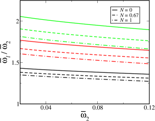
Figure 8: Plot of $\bar{\omega}_{l}/\bar{\omega}_{2}$ against $\bar{\omega}_{2}$ with $l=3$ (black lines), $l=4$ (red lines), and $l=5$ (green lines) for incompressible stars with $N=0$ (solid lines), and polytropic stars with $N=0.67$ (dashed lines) and $N=1.0$ (dot-dashed lines).

Finally, we remark that the present work is able to relate the multipole moments considered in the three-hair theorem (Yagi et al., 2014; Stein et al., 2014; Chatziioannou et al., 2014) to respective f-mode oscillation frequencies. Since the multipole moments of compact stars could be inferred by measuring the atomic spectra observed from such stars with future x-ray telescopes such as LOFT and NICER (Feroci et al., 2012; Gendreau et al., 2012), the relevant f-mode oscillation frequencies could likewise be derived from the $f$-$I$ universal formula.

References

- Weber (1999) F. Weber, Pulsars as Astrophysical Laboratories for Nuclear and Particle Physics (Institute of Physics, London, 1999).
- Lattimer and Prakash (2001) J. M. Lattimer and M. Prakash, Astrophys. J. 550, 426 (2001).
- Lattimer and Schutz (2005) J. M. Lattimer and B. F. Schutz, Astrophys. J. 629, 979 (2005).
- Lattimer and Prakash (2007) J. Lattimer and M. Prakash, Phys. Rep. 442, 109 (2007).
- Andersson and Kokkotas (1996) N. Andersson and K. D. Kokkotas, Phys. Rev. Lett 77, 4134 (1996).
- Andersson and Kokkotas (1998) N. Andersson and K. D. Kokkotas, Mon. Not. R. Astron. Soc. 299, 1059 (1998).
- Özel and Psaltis (2009) F. Özel and D. Psaltis, Phys. Rev. D 80, 103003 (2009).
- Ho et al. (2013) W. C. G. Ho, N. Andersson, C. M. Espinoza, K. Glampedakis, B. Haskell, and C. O. Heinke, Proc. Sci. ConfinementX (2012) 260 eprint [arXiv:1303.3282].
- Lattimer and Steiner (2014) J. M. Lattimer and A. W. Steiner, Euro. Phys. J. A 50, 40 (2014).
- Lattimer and Lim (2013) J. M. Lattimer and Y. Lim, Astrophys. J. 771, 51 (2013).
- Bejger and Haensel (2002) M. Bejger and P. Haensel, Astron. Astrophys. 396, 917 (2002).
- Burgay et al. (2003) M. Burgay et al., Nature (London) 426, 531 (2003).
- Lyne et al. (2004) A. G. Lyne et al., Science 303, 1153 (2004).
- Benhar et al. (1999) O. Benhar, E. Berti, and V. Ferrari, Mon. Not. R. Astron. Soc. 310, 797 (1999).
- Benhar et al. (2004) O. Benhar, V. Ferrari, and L. Gualtieri, Phys. Rev. D 70, 124015 (2004).
- Tsui and Leung (2005a) L. K. Tsui and P. T. Leung, Mon. Not. R. Astron. Soc. 357, 1029 (2005a).
- Tsui and Leung (2005b) L. K. Tsui and P. T. Leung, Astrophys. J. 631, 495 (2005b).
- Tsui and Leung (2005c) L. K. Tsui and P. T. Leung, Phys. Rev. Lett. 95, 151101 (2005c).
- Tsui et al. (2006) L. K. Tsui, P. T. Leung, and J. Wu, Phys. Rev. D 74, 124025 (2006).
- Lau et al. (2010) H. K. Lau, P. T. Leung, and L. M. Lin, Astrophys. J. 714, 1234 (2010).
- Gaertig and Kokkotas (2011) E. Gaertig and K. D. Kokkotas, Phys. Rev. D 83, 064031 (2011).
- Doneva et al. (2013) D. D. Doneva, E. Gaertig, K. D. Kokkotas, and C. Krüger, Phys. Rev. D 88, 044052 (2013).
- Punturo et al. (2010) M. Punturo et al., Class. Quant. Grav. 27, 194002 (2010).
- Yagi and Yunes (2013a) K. Yagi and N. Yunes, Phys. Rev. D 88, 023009 (2013a).
- Yagi and Yunes (2013b) K. Yagi and N. Yunes, Science 341, 365 (2013b).
- Urbanec et al. (2013) M. Urbanec, J. C. Miller, and Z. Stuchlík, Mon. Not. R. Astron. Soc. 433, 1903 (2013).
- Baubock et al. (2013) M. Baubock, E. Berti, D. Psaltis, and F. Ozel, Astrophys. J. 777, 68 (2013).
- Damour and Nagar (2009) T. Damour and A. Nagar, Phys. Rev. D 80, 084035 (2009).
- Yagi (2014) K. Yagi, Phys. Rev. D 89, 043011 (2014).
- Maselli et al. (2013) A. Maselli, V. Cardoso, V. Ferrari, L. Gualtieri, and P. Pani, Phys. Rev. D 88, 023007 (2013).
- Haskell et al. (2014) B. Haskell, R. Ciolfi, F. Pannarale, and L. Rezzolla, Mon. Not. R. Astron. Soc. 438, L71 (2014).
- Pappas and Apostolatos (2014) G. Pappas and T. A. Apostolatos, Phys. Rev. Lett. 112, 121101 (2014).
- Chakrabarti et al. (2014) S. Chakrabarti, T. Delsate, N. Gürlebeck, and J. Steinhoff, Phys. Rev. Lett. 112, 201102 (2014).
- Yagi et al. (2014) K. Yagi, K. Kyutoku, G. Pappas, N. Yunes, and T. A. Apostolatos, Phys. Rev. D 89, 124013 (2014).
- Stein et al. (2014) L. C. Stein, K. Yagi, and N. Yunes, Astrophys. J. 788, 15 (2014).
- Flanagan and Hinderer (2008) E. E. Flanagan and T. Hinderer, Phys. Rev. D 77, 021502 (2008).
- Hinderer (2008) T. Hinderer, Astrophys. J. 677, 1216 (2008).
- Sham et al. (2014) Y.-H. Sham, L.-M. Lin, and P. T. Leung, Astrophys. J. 781, 66 (2014).
- Pani and Berti (2014) P. Pani and E. Berti, Phys. Rev. D 90, 024025 (2014).
- Doneva et al. (2014) D. D. Doneva, S. S. Yazadjiev, N. Stergioulas, and K. D. Kokkotas, Astrophys. J. Lett. 781, L6 (2014).
- Kleihaus et al. (2014) B. Kleihaus, J. Kunz, and S. Mojica, Phys. Rev. D 90, 061501 (2014).
- Chandrasekhar (1963) S. Chandrasekhar, Astrophys. J. 139, 664 (1963).
- Press and Teukolsky (1977) W. H. Press and S. A. Teukolsky, Astrophys. J. 213, 183 (1977).
- Press (1971) W. Press, Astrophys. J. 170, L105 (1971).
- Leaver (1986) E. W. Leaver, Phys. Rev. D 34, 384 (1986).
- Ching et al. (1998) E. S. C. Ching, P. T. Leung, A. M. van den Brink, W. M. Suen, S. S. Tong, and K. Young, Rev. Mod. Phys. 70, 1545 (1998).
- Kokkotas and Schmidt (1999) K. D. Kokkotas and B. G. Schmidt, Living Rev. Relativity 2, 2 (1999).
- Berti et al. (2009) E. Berti, V. Cardoso, and A. O. Starinets, Classical Quantum Gravity 26, 163001 (2009).
- Postnikov et al. (2010) S. Postnikov, M. Prakash, and J. M. Lattimer, Phys. Rev. D 82, 024016 (2010).
- Hartle (1967) J. B. Hartle, Astrophys. J. 150, 1005 (1967).
- Hartle and Thorne (1968) J. B. Hartle and K. S. Thorne, Astrophys. J. 153, 807 (1968).
- Binnington and Poisson (2009) T. Binnington and E. Poisson, Phys. Rev. D 80, 084018 (2009).
- Chatziioannou et al. (2014) K. Chatziioannou, K. Yagi, and N. Yunes, Phys. Rev. D 90, 064030 (2014).
- Damour et al. (1992) T. Damour, M. Soffel, and C. Xu, Phys. Rev. D 45, 1017 (1992).
- Wiringa et al. (1988) R. B. Wiringa, V. Fiks, and A. Fabrocini, Phys. Rev. C 38, 1010 (1988).
- Lorenz et al. (1993) C. P. Lorenz, D. G. Ravenhall, and C. J. Pethick, Phys. Rev. Lett. 70, 379 (1993).
- Baldo et al. (1997) M. Baldo, I. Bombaci, and G. F. Burgio, Astron. Astrophys. 328, 274 (1997).
- Pandharipande and Ravenhall (1989) V. R. Pandharipande and D. G. Ravenhall, in Proceedings of the NATO Advanced Research Workshop on Nuclear Matter and Heavy Ion Collisions (Plenum, New York, 1989), p. 103.
- Johnson (1975) K. Johnson, Acta Phys. Pol. B 6, 865 (1975).
- Alcock et al. (1986) C. Alcock, E. Farhi, and A. Olinto, Astrophys. J. 310, 261 (1986).
- Witten (1984) E. Witten, Phys. Rev. D 30, 272 (1984).
- Chandrasekhar (1964) S. Chandrasekhar, Astrophys. J. 140, 417 (1964).
- Chandrasekhar (1965) S. Chandrasekhar, Astrophys. J. 142, 1519 (1965).
- Shapiro and Teukolsky (1983) S. L. Shapiro and S. A. Teukolsky, Black Holes, White Dwarfs, and Neutron Stars: The Physics of Compact Objects (Wiley, New York, 1983).
- Chodos et al. (1974) A. Chodos, R. L. Jaffe, K. Johnson, C. B. Thorne, and V. F. Weisskopf, Phys. Rev. D 9, 3471 (1974).
- Glendenning (1997) N. K. Glendenning, Compact Stars - Nuclear Physics, Particle Physics, and General Relativity (Springer, New York, 1997).
- Seidov and Kuzakhmedov (1978) Z. F. Seidov and R. K. Kuzakhmedov, Sov. Astron. 22, 711 (1978).
- Seidov (2004) Z. F. Seidov, eprint arXiv:astro-ph/0401359.
- Lake (2003) K. Lake, Phys. Rev. D 67, 104015 (2003).
- Lau (2009) H. K. Lau, Master’s thesis, The Chinese University of Hong Kong (2009).
- Chan (2012) T. K. Chan, Master’s thesis, The Chinese University of Hong Kong (2012).
- Cox (1980) J. Cox, Theory of Stellar Pulsation (Princeton University Press, 1980).
- Yagi et al. (2014) K. Yagi, L. C. Stein, G. Pappas, N. Yunes, and T. A. Apostolatos, Phys. Rev. D 90, 063010 (2014).
- Feroci et al. (2012) M. Feroci et al., Proc. SPIE 8433, 84432 (2012) .
- Gendreau et al. (2012) K. C. Gendreau, Z. Arzoumanian, and T. Okajima, Proc. SPIE 8443, 844313 (2012) .