Experimental implementation of adiabatic passage between different topological orders

Abstract

Topological orders are exotic phases of matter existing in strongly correlated quantum systems, which are beyond the usual symmetry description and cannot be distinguished by local order parameters. Here we report an experimental quantum simulation of the Wen-plaquette spin model with different topological orders in a nuclear magnetic resonance system, and observe the adiabatic transition between two $Z_{2}$ topological orders through a spin-polarized phase by measuring the nonlocal closed-string (Wilson loop) operator. Moreover, we also measure the entanglement properties of the topological orders. This work confirms the adiabatic method for preparing topologically ordered states and provides an experimental tool for further studies of complex quantum systems.

Over the past 30 years, it has become increasingly clear that the Landau symmetry-breaking theory cannot describe all phases of matter and their quantum phase transitions (QPTs) QPT ; Landau1937 ; Ginzburg1950 . The discovery of the fractional quantum Hall (FQH) effect TSG8259 indicates the existence of an exotic state of matter termed topological orders Wen1990TO , which are beyond the usual symmetry description. This type of orders has some interesting properties, such as robust ground state degeneracy that depends on the surface topology Wen1990TO2 , quasiparticle fractional statistics Arovas , protected edge states Wen1995 , topological entanglement entropy k3 and so on. Besides the importance in condensed matter physics, topological orders have also been found potential applications in fault-tolerant topological quantum computation k1 ; Nayak2008 ; Stern2013 . Instead of naturally occurring physical systems (e.g., FQH), two-dimensional spin-lattice models, including the toric-code model k1 , the Wen-plaquette model Wen2003 , and the Kitaev model on a hexagonal lattice k2 , were found to exhibit $Z_{2}$ topological orders. The study of such systems therefore provides an opportunity to understand more features of topological orders and the associated topological QPTs p3 ; HammaPRL2008 ; HammaPRB2008 . A large body of theoretical work exists on these systems, including several proposals for their physical implementation in cold atoms Duan2003 , polar molecules Micheli2006 or arrays of Josephson junctions You2010 . However, only a very small number of experimental investigations have actually demonstrated such topological properties (e.g., anyonic statistics and robustness) using either photons Pan2012 or nuclear spins Du2007 . However, in these experiments, specific entangled states having topological properties have been dynamically generated, instead of direct Hamiltonian engineering and ground-state cooling which are extremely demanding experimentally.

Rather than the toric-code model, the first spin-lattice model with topological orders, here we study an alternative exactly solvable spin-lattice model – the Wen-plaquette model Wen2003 . Two different $Z_{2}$ topological orders exist in this system; their stability depends on the sign of the coupling constants of the four-body interaction. Between these two phases, a new kind of phase transition occurs when the couplings vanish. So far, neither these topological orders nor this topological QPT have been observed experimentally. The two major challenges are (i) to engineer and to experimentally control complex quantum systems with four-body interactions and (ii) to detect efficiently the resulting topologically ordered phases. Along the lines suggested by Feynman Feynman1982 , complex quantum systems can be efficiently simulated on quantum simulators, i.e., programmable quantum systems whose dynamics can be efficiently controlled. Some earlier experiments have been studied, e.g., in condensed-matter physics Pan2012 ; Du2007 ; Peng2005 and quantum chemistry Lu2011 (see the review on quantum simulation QSreview and references therein). Quantum simulations thus offer the possibility to investigate strongly correlated systems exhibiting topological orders and other complex quantum systems that are challenging for simulations on classical computers.

In this Letter, we demonstrate an experimental quantum simulation of the Wen-plaquette model in a nuclear magnetic resonance (NMR) system and observe an adiabatic transition between two different topological orders that are separated by a spin-polarized state. To the best of our knowledge, this is the first experimental observation of such a system based on using the Wilson loop operator, which corresponds to a nonlocal order parameter of a topological QPT HammaPRL2008 ; HammaPRB2008 . Both topological orders are further confirmed to be highly entangled by quantum state tomography. The experimental adiabatic method paves the way towards constructing and initializing a topological quantum memory Dennis2002 ; Jiang2008 .

We focus on the Wen-plaquette model Wen2003 shown in Fig. 1(a), an exactly solvable quantum spin model with $Z_{2}$ topological orders. It is described by the Hamiltonian

$$\hat{H}_{Wen}=-J\sum_{i}\hat{F_{i}},$$ (1)

where $\hat{F_{i}}=\hat{\sigma}_{i}^{x}\hat{\sigma}_{i+\hat{e}_{x}}^{y}\hat{\sigma}_{i+\hat{e}_{x}+\hat{e}_{y}}^{x}\hat{\sigma}_{i+\hat{e}_{y}}^{y}$ is the plaquette operator that acts on the four spins surrounding a plaquette. Since $\hat{F_{i}}^{2}=1$, the eigenvalues of $\hat{F_{i}}$ are $F_{i}=\pm 1$. We see that when $J>0$ the ground state has all $F_{i}=1$ and when $J<0$ the ground state has all $F_{i}=-1$. According to the classification of the projective symmetry group Wen2003 , they correspond to two types of topological orders: $Z_{2}A$ and $Z_{2}B$ order, respectively. It is obvious that both topological orders have the same global symmetry as that belongs to the Hamiltonian. So one cannot use the concept of “spontaneous symmetry breaking” and the local order parameters to distinguish them. In $Z_{2}A$ $(Z_{2}B)$ order, a “magnetic vortex” (or $m$-particle) is defined as $F_{i}=-1$ ($F_{i}=1$) at an even sub-plaquette and an “electric charge” (or $e$-particle) is $F_{i}=-1$ ($F_{i}=1$) at an odd sub-plaquette WenPRD2003 . Due to the mutual semion statistics between $e$- and $m$-particles, their bound states obeys fermionic statistics k2 ; WenPRD2003 . Physically, in $Z_{2}B$ topological order, a fermionic excitation (the bound state of $e$ and $m$) sees a $\pi$-flux tube around each plaquette and acquires an Aharonov–Bohm phase $e^{i\pi}$ when moving around a plaquette, while in $Z_{2}A$ topological order, the fermionic excitation feels no additional phase when moving around each plaquette. Thus the transition at $J=0$ represents a new kind of phase transition that changes quantum orders but not symmetry Wen2003 ; WenPRD2003 .

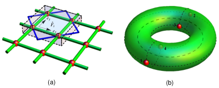
Figure 1: (Color online.) (a) Wen-plaquette model. The red spheres represent spin-$1/2$ particles. The plaquette operator is $\hat{F_{i}}=\hat{\sigma}_{i}^{x}\hat{\sigma}_{i+\hat{e}_{x}}^{y}\hat{\sigma}_{i+\hat{e}_{x}+\hat{e}_{y}}^{x}\hat{\sigma}_{i+\hat{e}_{y}}^{y}$. The closed string (blue) represents the Wilson loop in a $2\times 2$ lattice. (b) A torus formed from a $2\times 2$ lattice (labeled by 1,2 3,4) with periodic boundary condition.

However, it is difficult to directly observe the transition from $Z_{2}A$ to $Z_{2}B$ topological order in the experiment, because the energies of all quantum states are zero at the critical point. Instead, the Wen-plaquette model in a transverse field

$$\hat{H}_{tol}=\hat{H}_{Wen}-g\sum_{i}\hat{\sigma_{i}^{x}}.$$ (2)

is often studied p3 ; HammaPRL2008 ; HammaPRB2008 . Without loss of generality, we consider the case $g>0$. Figure 2 shows its 2D phase diagram, which contains three regions in which the ground state is $Z_{2}B$ order when $J\ll-g$, $Z_{2}A$ order when $J\gg g$ and a spin-polarized state without topological order when $|J|\ll g$, respectively. From Fig. 2, we can see that by changing $J$, the ground state of the system is driven from $Z_{2}A$ to $Z_{2}B$ topological order through the trivial spin-polarized state. The spin-polarized region from one topological order to the other one depends on the size of the transverse field strength $g$: the smaller $g$ is, the narrower the region of spin-polarized state becomes. If $g$ vanishes (or $J$ is large enough), a QPT occurs between the two types of topological orders Wen2003 . The above results are valid only for infinite systems. For finite systems, the situation is more complicated. For example, the topological degeneracies of the system depend on the type of the lattice (even-by-even, even-by-odd, odd-by-odd lattices). However, the properties of the topological orders persist in the Wen-plaquette model with finite-size lattices Wen2003 .

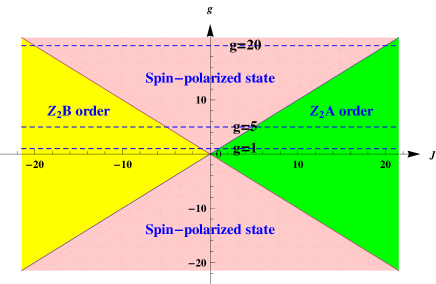
Figure 2: (Color online.) 2D phase diagram of Wen-plaquette model in a transverse field. The yellow, green and pink regions represent $Z_{2}B$, $Z_{2}A$ topological orders, and the spin-polarized state, respectively. The three dashed lines correspond to the tested values of $g=1,g=5$ and $g=20$ in the experiment.

The simplest finite system that exhibits topological orders consists of a $2\times 2$ lattice with periodic boundary condition, as shown in Fig. 1(b). The Hamiltonian can be described as

$$\hat{H}_{Wen}^{4}=-2J(\hat{\sigma}_{1}^{x}\hat{\sigma}_{2}^{y}\hat{\sigma}_{3}^{x}\hat{\sigma}_{4}^{y}+\hat{\sigma}_{1}^{y}\hat{\sigma}_{2}^{x}\hat{\sigma}_{3}^{y}\hat{\sigma}_{4}^{x}).$$ (3)

The fourfold degeneracy of the ground states is a topological degeneracy and the two ground states for $J<0$ and for $J>0$ have different quantum orders Wen2003 . Adding a transverse field, we obtain the transverse Wen-plaquette model $\hat{H}_{tol}$ in Eq. (7) for the finite system, where the degeneracy is partly lifted p3 . For the case $g>0$, the non-degenerate ground state is:

$$|\psi_{g}\rangle\approx\left\{\begin{array}[]{ll}|\psi_{Z_{2}B}\rangle=|\phi^{+}\rangle_{13}|\phi^{+}\rangle_{24},&J\ll-g<0\\ |\psi_{SP}\rangle=|++++\rangle,&J=0\\ |\psi_{Z_{2}A}\rangle=|\psi^{+}\rangle_{13}|\psi^{+}\rangle_{24},&J\gg g>0\end{array}\right..$$ (4)

Here $|\phi^{+}\rangle=\frac{1}{\sqrt{2}}(|00\rangle+|11\rangle)$, $|\psi^{+}\rangle=\frac{1}{\sqrt{2}}(|01\rangle+|10\rangle)$ and $|+\rangle=\frac{1}{\sqrt{2}}(|0\rangle+|1\rangle)$. The energy-level diagram and the ground state are given in Ref. SM . Eq. (4) shows that both topological orders are symmetric and possess bipartite entanglement, while the spin-polarized state $|\psi_{SP}\rangle$ is a product state without entanglement.

The physical four-qubit system we used in the experiments consists of the nuclear spins in Iodotrifluroethylene (C₂F₃I) molecules with one ¹³C and three ¹⁹F nuclei. Figure  3 (a) and (b) show its molecular structure and relevant properties SM . The natural Hamiltonian of this system in the doubly rotating frame is

$$\hat{H}_{NMR}=\sum_{i=1}^{4}\frac{\omega_{i}}{2}\hat{\sigma}^{z}_{i}+\sum_{i<j,=1}^{4}\frac{\pi J_{ij}}{2}\hat{\sigma}^{z}_{i}\hat{\sigma}^{z}_{j},$$ (5)

where $\omega_{i}$ represents the chemical shift of spin $i$ and $J_{ij}$ the coupling constant. The experiments were carried out on a Bruker AV-400 spectrometer ($9.4T$) at room temperature $T=300$ K. The temperature fluctuation was controlled to $<0.1$ K, which results in a frequency stability within $1$ Hz. Figure 3(c) shows the quantum circuit for the experiment, which can be divided into three steps: ($i$) preparation of the initial ground state of the Hamiltonian $\hat{H}_{tol}[J(0)]$ for a given transverse field $g$, ($ii$) adiabatic simulation of $\hat{H}_{tol}[J(t)]$ by changing the control parameter $J$ from $J(0)$ to $J(T)$, and ($iii$) detection of the resulting state.

Figure 3: (Color online.) (a) Molecular structure of lodotrifluroehtylene. One ¹³C and three ¹⁹F nuclei are used as a four-qubit quantum simulator. (b) Relevant parameters measured at $T=300K$. The diagonal and nondiagonal elements represent the chemical shifts and the coupling constants in units of Hz, respectively. The measured spin-lattice relaxation times ($T_{1}$) are $21$ s for ¹³C and $12.5$ s for ¹⁹F. (c) Quantum circuit for observing the topological-order-transition in the Wen-plaquette model. $X$ and $\bar{Y}$ represent $\frac{\pi}{2}$ rotations of single qubits around the $x$ and $-y$ axes, respectively.

To prepare the system in the ground state, we used the technique of pseudo-pure states (PPS): $\hat{\rho}_{\psi}=\frac{1-\epsilon}{16}\mathbf{I}+\epsilon|\psi\rangle\langle\psi|$, with $\mathbf{I}$ representing the $16\times 16$ identity operator and $\epsilon\approx 10^{-5}$ the polarization. Starting from the thermal state, we prepared the PPS $\hat{\rho}_{0000}$ by line-selective pulses Peng2001 . The experimental fidelity of $\hat{\rho}_{0000}$ defined by $|Tr(\hat{\rho}_{th}\hat{\rho}_{exp})|/\sqrt{Tr(\hat{\rho}_{th}^{2})Tr(\hat{\rho}_{exp}^{2})}$ was around $97.7\%$. Then we obtained the initial ground state $\hat{\rho}_{\psi_{g}}$ of $\hat{H}_{tol}[J(0)]$ by a unitary operator realized by a GRAPE pulse Glaser2005 with a duration of 6 ms.

To observe the ground-state transition, we implemented an adiabatic transfer from $\hat{H}_{tol}[J(0)]$ to $\hat{H}_{tol}[J(T)]$ Messiah1976 . The sweep control parameter $J(t)$ was numerically optimized and implemented as a discretised scan with $M$ steps :

$$\hat{U}_{ad}=\prod_{m=1}^{M}\hat{U}_{m}[J_{m}]=\prod_{m=1}^{M}e^{-i\hat{H}_{tol}[J_{m}]\tau},$$ (6)

where the duration of each step is $\tau=T/M$. The adiabatic limit corresponds to $T,M\rightarrow\infty,\tau\rightarrow 0$. Using $M=31$, the optimized sweep reaches a theoretical fidelity $>99.5$% of the final state with respect to the true ground state. For each step of the adiabatic passage, we designed the NMR pulse sequence to create an effective Hamiltonian, i.e., $\hat{H}_{tol}[J_{m}]$ SM .

In the experiment, we employed the Wilson loop HammaPRL2008 ; HammaPRB2008 ; Kogut1979 to detect the transition between two different topological orders. The effective theory of topological orders is a $Z_{2}$ gauge theory and the observables must be gauge invariant quantities. The Wilson loop operator is gauge invariant and can be as a nonlocal order parameter. It is defined as $\hat{W}(C)=\prod_{C}\hat{\sigma}_{i}^{\alpha_{i}}$, where the product $\prod_{C}$ is over all sites on the closed string $C$, $\alpha_{i}=y$ if $i$ is even and $\alpha_{i}=x$ if $i$ is odd WenPRD2003 . For the $2\times 2$ lattice system, this corresponds to $\hat{W}(C)=\hat{\sigma}_{1}^{x}\hat{\sigma}_{2}^{y}\hat{\sigma}_{3}^{x}\hat{\sigma}_{4}^{y}$. The experimental results of $\langle\hat{W}(C)\rangle$ can be obtained by recording the carbon spectra after a read-out pulse $[\frac{\pi}{2}]_{x}^{F_{1}}[\frac{\pi}{2}]_{\bar{y}}^{F_{2}}[\frac{\pi}{2}]_{x}^{F_{3}}$. Figure 4(a) shows the resulting data for three sets of experiments with $g=1,$ $g=5$, $g=20$ and $J$ varying from $-20$ to $20$. When $|J/g|\gg 1$, $\langle\hat{W}(C)\rangle$ is close to $\pm 1$, corresponding to $Z_{2}A$/$Z_{2}B$ topological order. The results shown in figure 4(a) verify that the transition region becomes narrower and sharper as $g$ decreases. In the absence of the transverse field, $g\to 0$, the ground state makes a sudden transition at $J=0$ from $Z_{2}B$ to $Z_{2}A$ topological order. This is a novel QPT between different topological orders Wen2003 . These results also show that the Wilson loop is a useful nonlocal order parameter that characterises the different $Z_{2}$ topological orders very well.

To demonstrate more clearly that this topological QPT goes beyond Landau symmetry-breaking theory and cannot be described by local order parameters, we also measured the single-particle operator of the ¹³C spin:

$$P=|Tr[\hat{\rho}_{f}(\hat{\sigma}_{1}^{x}-i\hat{\sigma}_{1}^{y})]|=\sqrt{Tr(\hat{\rho}_{f}\hat{\sigma}_{1}^{x})^{2}+Tr(\hat{\rho}_{f}\hat{\sigma}_{1}^{y})^{2}}.$$

This was performed by measuring the magnitude of the ¹³C NMR signal while decoupling ¹⁹F. Here $\hat{\rho}_{f}$ is the final state at the end of the adiabatic scan. Due to the symmetry of the Hamiltonian, the values of $P$ are equal for all the four spins. Figure 4(b) shows the experimental results. They are symmetric with respect to $J=0$, which means that the different $Z_{2}$ topological orders cannot be distinguished by the local order parameter.

By performing complete quantum state tomography Lee , we reconstructed the density matrices for $Z_{2}B$ order ($J=-20$), for the spin-polarized state ($J=0$) and $Z_{2}A$ order ($J=20$) for $g=1$. The real parts of these density matrices are shown in Fig.4(c), (d) and (e). The experimental fidelities are $95.2\%,$ $95.6\%$ and $95.7\%$, respectively. From these reconstructed density matrices, we also calculated the entanglement: for both topological orders, $C(\hat{\rho}_{13}^{exp})\approx C(\hat{\rho}_{24}^{exp})\approx 0.89$, while the others were close to 0; for the spin-polarized state, all $C(\hat{\rho}_{ij}^{exp})$ are almost zero. Here $\hat{\rho}_{ij}^{exp}$ is the reduced density matrix of two spins $i,j$ obtained by partially tracing out the other spins from the experimentally reconstructed density matrix $\hat{\rho}^{exp}$ and the concurrence is defined as $C(\hat{\rho}_{ij}^{exp})=max\{\lambda_{1}-\lambda_{2}-\lambda_{3}-\lambda_{4},0\}$, where $\lambda_{k}$s (in decreasing order) are the square roots of the eigenvalues of $\hat{\rho}_{ij}^{exp}(\hat{\sigma}^{y}_{i}\hat{\sigma}^{y}_{j})\hat{\rho}_{ij}^{exp^{\ast}}(\hat{\sigma}^{y}_{i}\hat{\sigma}^{y}_{j})$Wootters1998 . Therefore, the topological orders exhibit the same bipartite entanglement between qubits 1, 3 and 2, 4 in agreement with Eq. (4). These experimental results are in good agreement with theoretical expectations. The relatively minor deviations can be attributed mostly to the imperfections of the GRAPE pulses, the initial ground state preparation and the spectral integrals SM .

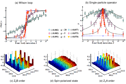
Figure 4: (Color online.) (a) Measured expectation values of the nonlocal string operator – the Wilson loop $\langle\hat{W}(C)\rangle$. (b) Measured values $P$ of the local single-particle operator. The experimental points are denoted by the symbols $\triangledown$, $\lozenge$ and $\circ$ for $g=1,g=5$ and $g=20$, respectively, along with the theoretical expectations denoted by the black solid lines. The error bars indicate the standard deviations of the experimental measurements. The sharp transition denoted by the blue dashed line is the theoretical expectation when $g=0$. (c) (d) and (e) Real parts of experimentally reconstructed density matrices for the ground states with $g=1$ at $J=-20$, $J=0$ and $J=20$, corresponding to $Z_{2}B$ topologically ordered state $|\psi_{Z_{2}B}\rangle$, spin-polarized state $|\psi_{SP}\rangle$ and $Z_{2}A$ topologically ordered state $|\psi_{Z_{2}A}\rangle$. All imaginary parts of the density matrices are small. The rows and columns represent the standard computational basis in binary order, from $|0000\rangle$ to $|1111\rangle$.

Instead of studying naturally existing topological phases like those in quantum Hall systems, lattice-spin models can be designed to exhibit interesting topological phases. One example is the Wen-plaquette model, which includes many-body interactions. Such interactions have not been found in naturally occurring systems, but they can be generated as effective interactions in quantum simulators. Using an NMR quantum simulator, we provide a first proof-of-principle experiment that implements an adiabatic transition between two different $Z_{2}$ topological orders through a spin-polarized state in the transverse Wen-plaquette model. Such models are beyond Landau symmetry-breaking theory and cannot be described by local order parameters. Ref. HammaPRB2008 presented a numerical study of a QPT from a spin-polarized to a topologically ordered phase using a variety of previously proposed QPT detectors and demonstrated their feasibility. Furthermore, we also demonstrated in an experiment that the nonlocal Wilson loop operator can be a nontrivial detector of topological QPT between different topological orders. This phenomenon requires further investigation to be properly understood.

Although a $2\times 2$ lattice is a very small finite-size system, topological orders exist in the Wen-plaquette model with periodic lattice of finite size Wen2003 . The validity of the quantum simulation of the topological orders in such a small system also comes from the fairly short-range spin-spin correlations. When $|g/J|\leq 1$, all quasi-particles (the electric charges, magnetic vortices and fermions) perfectly localize that leads to zero spin-spin correlation length k1 ; Yu2009 . Therefore the topological properties of the ground state persist in such a small system, including the topological degeneracy, the statistics of the quasi-particles and the non-zero Wilson loop SM . The present method can in principle be expanded to larger systems with more spins, which allows one to explore more interesting physical phenomena, such as lattice-dependent topological degeneracy Wen2003 , quasiparticle fractional statistics Arovas ; k2 and the robustness of the ground state degeneracy against local perturbations Wen1990TO2 ; HammaPRL2008 ; HammaPRB2008 ; Yu2009 . Quantum simulators using larger spin systems can be more powerful than classical computers and permit the research of topological orders and their physics beyond the capabilities of classical computers. Nevertheless, our present experimental results demonstrate the feasibility of small quantum simulators for strongly correlated quantum systems, and the usefulness of the adiabatic method for constructing and initializing a topological quantum memory.

We thanks L. Jiang and C. K. Duan for the helpful discussion. This work is supported by NKBRP (973 programs 2013CB921800, 2014CB848700, 2012CB921704, 2011CB921803), NNSFC (11375167, 11227901, 891021005), CAS (SPRB(B) XDB01030400), RFDPHEC (20113402110044).

I Supplementary Materials

II Theoretical calculations in the transverse Wen-Plaquette model

II.1 Energy levels and ground state

With periodic boundary condition, the total Hamiltonian of 2 by 2 lattices in the transverse Wen-Plaquette model is

$$\hat{H}_{tol}=-2J(\hat{\sigma}_{1}^{x}\hat{\sigma}_{2}^{y}\hat{\sigma}_{3}^{x}\hat{\sigma}_{4}^{y}+\hat{\sigma}_{1}^{y}\hat{\sigma}_{2}^{x}\hat{\sigma}_{3}^{y}\hat{\sigma}_{4}^{x})-g\sum_{i}^{4}\hat{\sigma}_{i}^{x}.$$ (7)

In the representation of $\hat{\sigma_{x}}$ basis, its ground state is

$$|\psi_{g}\rangle=\frac{1}{\sqrt{A}}[\alpha_{1}|0000\rangle_{x}-\alpha_{2}\frac{|0101\rangle_{x}+|1010\rangle_{x}}{\sqrt{2}}+\alpha_{3}|1111\rangle_{x}],$$

where $A$ is the normalization constant and $\alpha_{1}=J^{2}+2g^{2}+2g\sqrt{g^{2}+J^{2}},$ $\alpha_{2}=\sqrt{2}J(g+\sqrt{g^{2}+J^{2}})$ and $\alpha_{3}=J^{2}$. The corresponding ground-state energy is

$$\varepsilon=-4\sqrt{g^{2}+J^{2}}.$$ (8)

Figure 5 shows its energy-level diagram and the probability amplitudes of the ground state $|\psi_{g}\rangle$ as a function of the four-body interaction strength $J$ for a transverse field (here we take $g=1$). The energy-level diagram is symmetry about $J=0$ because of the symmetric transverse field. When $|J/g|\gg 1$, the ground state is progressively four-fold degeneracy (the full four-fold degeneracy of ground state when $g=0$ is partially lifted when $g\neq 0$, see the subplot of Fig.  5(a)). Note that the ground-state energy seems to be smooth due to the scale-size effect and the transverse field. For the Wen-Plaquette model (i.e. g = 0), an actual level-crossing in the four-spin system creates a point of nonanalyticity of the ground state energy as a function of the control parameter $J$. As theoretically predicted by X. Wen Wen2003 , a quantum phase transition (QPT) between two different topological orders ($Z_{2}A$ and $Z_{2}B$ orders) occurs at $J=0$. However, the transition cannot be directly observed in experiment due to the level-crossing (the adiabatic passage will fail at the transition point). Therefore, we turn to the transverse Wen-Plaquette model (i.e., $g\neq 0$), where a second-order QPT between one topological order and spin-polarized state occurs at $J/g=\pm 1$ in the thermodynamic limit Yu2008 ; Feng2007 ; HammaPRL2008 ; HammaPRB2008 . Accordingly, these two topological orders ($Z_{2}A$ and $Z_{2}B$ orders) are connected by a spin-polarized state, as shown in Fig. 2 in the paper. The region of spin-polarized state will become narrow as $|g/J|$ decreases. When $g/J\to 0$, the region turns into a point, and the ground-state transition in the Wen-Plaquette model Wen2003 can be asymptotically observed in the experiment. Therefore, as long as $g$ is small enough, the main features of the ground state in Wen-plaquette model persists (except for the point of $J=0$). As shown in Figure 5(b), it clearly illustrates that there are two different types of the entangled ground states for $J\gg 1$ and $J\ll-1$.

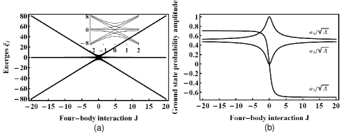
Figure 5: (a) Energy-level diagram of 2 by 2 lattices in the transverse Wen-plaquette model when $g=1$. (b) Probability amplitudes $(\alpha_{i}/\sqrt{A},i=1,2,3.)$ of ground state $|\psi_{g}\rangle$ for $g=1$.

II.2 Spin-spin correlations

The validity of the quantum simulation of the topological orders in the Wen-plaquette model on $2$-by-$2$ lattice comes from the fairly short range spin-spin correlations. For the Wen-plaquette model in the exactly solvable limit ($g/J\rightarrow 0$) all quasi-particles (the electric charges, magnetic vortices and fermions) have flat bands. In other words, the quasi-particles cannot move at all. Such perfect localization of quasi-particles leads to no spin-spin correlations for two spins on different sites, $\langle\hat{\sigma}_{i}^{x}\hat{\sigma}_{j}^{x}\rangle=\langle\hat{\sigma}_{i}^{y}\hat{\sigma}_{j}^{y}\rangle=\langle\hat{\sigma}_{i}^{z}\hat{\sigma}_{j}^{z}\rangle=0$ for $i\neq j$. Under the perturbations, the quasi-particles begin to hop. For example, the term $g\sum_{i}\hat{\sigma_{i}^{x}}$ drives the quasi-particles hopping along diagonal direction k1 ; KouPRL2009 ; Yu2009 . Therefore one may manipulate the dynamics of the quasi-particles by adding the external field and consequently control the spin-spin correlation length $\xi$.

By using the exact diagonalization technique of the Wen-plaquette model on a $2$-by-$6$ lattices with periodic boundary condition, we obtain the spin-spin correlations for two spins with different distances via the strength of the external field $g$. See the results in Fig. 6. From this figure, one can see that in the region of $g/J<1$, the spin-spin correlation length is always smaller than $2$. As a result, for the Wen-plaquette model on $2$-by-$2$ lattice, we can also get the topological properties including the topological degeneracy, the statistics of the quasi-particles and the non-zero Wilson loop. For example, the energy splitting of the degenerate ground states is estimated by $\Delta E\sim e^{-L/\xi}$ where $L$ is size of the systemk1 ; KouPRL2009 ; Yu2009 . In the limit of $g/J\rightarrow 0$, due to perfect localization, $\xi\rightarrow 0$, for the Wen-plaquette model on $2$-by-$2$ lattice the energy splitting of the degenerate ground states disappears, $\Delta E\sim e^{-L/\xi}\rightarrow 0$ ($L=2$). However, in the region of $g/J>1$, the ground state is spin-polarized phase without topological order, of which the spin-spin correlation length is infinite. Due to its trivial properties, we can also simulate the system on a lattice of small size.

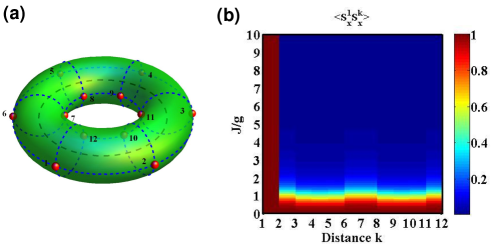
Figure 6: (a)The Wen-plaquette model on a $2\times 6$ lattices with periodic condition and (b)the spin-spin correlation of $\langle S_{x}^{1}S_{x}^{k}\rangle$ vs distance k and the ratio of $J/g$.

III Experimental procedure

III.1 Quantum simulator and characterization

We chose the ¹³C, and three ¹⁹F nuclear spins of iodotrifluoroethyene dissolved in d-chloroform as a four-qubit quantum simulator. The exact characterization of the quantum simulator is very important for precise quantum control in the experiments. The transverse relaxation times were measured by the CPMG pulse sequence. The absolute values of the J-coupling constants were obtained from the equilibrium spectrum. We determined their relative sign by creating observable three-spin orders, such as $I_{1}^{x}I_{2}^{z}I_{3}^{z}$ and measuring the 1-D NMR spectrum. This method requires a simpler pulse sequence and less experimental time than 2D NMR sequences like $\beta$-COSY Claridge . Because we used an unlabeled sample, the molecules with a ¹³C nucleus, which we used as the quantum register, were present at a concentration of about $1\%$. The ¹⁹F spectra were dominated by signals from the three-spin molecules containing the ¹²C isotope, while the signals from the quantum simulator with the ¹³C nucleus appeared only as small ($0.5\%$) satellites. The accurate ¹⁹F chemical shifts are thus hidden in the very small signals, which are obtained by exact assignments to distinguish them from spurious molecules with a ¹³C nucleus.

III.2 Adiabatic passage

We simulated the adiabatic transition from a topological ordered state to another one through a spin-polarized state, where the four-body interaction $J$ was adiabatically driven as a control parameter. To ensure that the system always stays in the instantaneous ground state, the variation of the control parameter has to be sufficiently, i.e., the adiabatic condition Messiah1976

$$\bigg{|}\frac{\langle\psi_{g}|\dot{\psi}_{e}\rangle}{\varepsilon_{e}-\varepsilon_{g}}\bigg{|}\ll 1$$ (9)

is satisfied, where the index $e$ represents the excited state. The condition can be rewritten as

$$\bigg{|}\frac{dJ(t)}{dt}\bigg{|}\ll 1/\bigg{|}\frac{\langle\psi_{g}|\frac{\partial\hat{H}_{tol}}{\partial J}|\psi_{e}\rangle}{(\varepsilon_{e}-\varepsilon_{g})^{2}}\bigg{|}.$$ (10)

Equation (10) determines the optimal sweep of control parameter $J(t)$, denoted by solid line in Fig. 7(a). For the experimental implementation, we discretized the time-dependent parameter $J(t)$ into $M$ segments during the total duration of the adiabatic passage $T$. The adiabatic condition is satisfied when both $T,M\to\infty$ and the duration of each step $\tau\to 0$. To determine the optimal number $M$ of steps in the adiabatic transfer, we used a numerical simulation of the minimum fidelity $F_{min}$ encountered during the scan as a function of the number of steps into which the evolution is divided (see Fig. 7(b)), where we fixed the total evolution time $T=6.5684$. The fidelity is calculated as the overlap of the state with the ground state at the relevant position. When $M=31$, the minimal fidelity is 0.995, which fully indicates the state of the system is always close to its instantaneous ground state in the whole adiabatic passage.

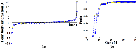
Figure 7: (a) Adiabatic four-body-interaction sweep $J(t)$. The solid line was calculated for constant adiabaticity parameter [see Eq. (5)] for a transverse field $g=1$. The $\bigtriangledown$ points represent the $M=31$ interpolations on the solid line for the discretized scan. (b) Numerical simulation of the minimum fidelities during the adiabatic passage vs. the number of steps.

III.3 Experimental Hamiltonian Simulation of the transverse Wen-plaquette model

Using Trotter’s formula, the target Hamiltonian (the transverse Wen-plaquette model in Eq. (1)) can be created as an average Hamiltonian by concatenating evolutions with short periods

$$e^{-i\hat{H}_{tol}\tau}=e^{-i\hat{H}_{x}\tau/2}e^{-i\hat{H}_{Wen}^{4}\tau}e^{-i\hat{H}_{x}\tau/2}+O(\tau^{3}),$$

where $\hat{H}_{x}=-g\sum_{j=1}^{4}\hat{\sigma}_{x}^{j}$ and $\hat{H}_{Wen}^{4}=-2J(\hat{\sigma}_{1}^{x}\hat{\sigma}_{2}^{y}\hat{\sigma}_{3}^{x}\hat{\sigma}_{4}^{y}+\hat{\sigma}_{1}^{y}\hat{\sigma}_{2}^{x}\hat{\sigma}_{3}^{y}\hat{\sigma}_{4}^{x})$. This expansion faithfully represents the targeted evolution provided the duration $\tau$ is kept sufficiently short. Due to $[\hat{\sigma}_{1}^{x}\hat{\sigma}_{2}^{y}\hat{\sigma}_{3}^{x}\hat{\sigma}_{4}^{y},\hat{\sigma}_{1}^{y}\hat{\sigma}_{2}^{x}\hat{\sigma}_{3}^{y}\hat{\sigma}_{4}^{x}]=0$,

$$e^{-i\hat{H}_{Wen}^{4}\tau}=\bar{Y}_{1}\bar{X}_{2}\bar{Y}_{3}\bar{X}_{4}e^{-i2J\hat{\sigma}_{1}^{z}\hat{\sigma}_{2}^{z}\hat{\sigma}_{3}^{z}\hat{\sigma}_{4}^{z}\tau}Y_{1}X_{2}Y_{3}X_{4}$$

$$\cdot\bar{X}_{1}\bar{Y}_{2}\bar{X}_{3}\bar{Y}_{4}e^{-i2J\hat{\sigma}_{1}^{z}\hat{\sigma}_{2}^{z}\hat{\sigma}_{3}^{z}\hat{\sigma}_{4}^{z}\tau}X_{1}Y_{2}X_{3}Y_{4}.$$

Here the many-body interaction can be simulated by a combination of two-body interactions and RF pulses Tseng1999 ; Peng2009 :

$$e^{-i2J\sigma_{z}^{1}\sigma_{z}^{2}\sigma_{z}^{3}\sigma_{z}^{4}\tau}$$

$$=e^{-i(\theta_{1}\hat{\sigma}_{z}^{1}+\theta_{2}\hat{\sigma}_{z}^{2}+\theta_{3}\hat{\sigma}_{z}^{4})/2}Y_{3}e^{-i\hat{H}_{\text{NMR}}\tau_{1}}e^{-i\pi(\hat{\sigma}_{y}^{3}+\hat{\sigma}_{y}^{4})/2}$$

$$\cdot e^{-i\hat{H}_{\text{NMR}}\tau_{1}}\bar{Y}_{1}\bar{X}_{3}e^{-i\hat{H}_{\text{NMR}}\tau_{2}}e^{-i\pi(\hat{\sigma}_{y}^{1}+\hat{\sigma}_{y}^{2})/2}e^{-i\hat{H}_{\text{NMR}}\tau_{2}}$$

$$\cdot X_{1}e^{-i\hat{H}_{\text{NMR}}\tau_{3}}e^{-i\pi(\hat{\sigma}_{x}^{1}+\hat{\sigma}_{x}^{3})/2}e^{-i\hat{H}_{\text{NMR}}\tau_{3}}X_{1}e^{-i\hat{H}_{\text{NMR}}\tau_{2}}$$

$$\cdot e^{-i\pi(\hat{\sigma}_{y}^{1}+\hat{\sigma}_{y}^{2})/2}e^{-i\hat{H}_{\text{NMR}}\tau_{2}}\bar{Y}_{1}X_{3}e^{-i\pi\hat{\sigma}_{y}^{2}/2}e^{-i\hat{H}_{\text{NMR}}\tau_{1}}$$

$$\cdot e^{-i\pi(\hat{\sigma}_{x}^{3}+\hat{\sigma}_{x}^{4})/2}e^{-i\hat{H}_{\text{NMR}}\tau_{1}}Y_{3}$$

Figure 8 shows the pulse sequences for simulating the transverse Wen-plaquette model of Eq. (1). The simulation method is in principle efficient as long as the decoherence time is long enough.

In order to overcome the accumulated pulse errors and the decoherence, we packed the adiabatic passage for each $J(m)$ ($m=0,1,2,...,M-1$) into one shaped pulse calculated by the gradient ascent pulse engineering (GRAPE) method Glaser2005 , with the length of each pulse being 30 ms. All the pulses have theoretical delities over 0.995, and are designed to be robust against the inhomogeneity of radio-frequency pulses in the experiments. As an example, we show a GRAPE pulse in Fig. 9.

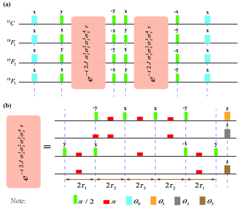
Figure 8: Pulse sequences for (a) simulating the transverse Wen-plaquette model of Eq. (1), and (b) four-body interaction, i.e., $\hat{\sigma}_{z}^{1}\hat{\sigma}_{z}^{2}\hat{\sigma}_{z}^{3}\hat{\sigma}_{z}^{4}$, where $\tau_{1}=1/4J_{34},\tau_{2}=1/4J_{12},\tau_{3}=2J\tau/\pi J_{13},\theta_{0}=-g\tau,\theta_{1}=-\omega_{1}/J_{34},\theta_{2}=-4\omega_{2}J\tau/\pi J_{13}$ and $\theta_{3}=\omega_{4}/J_{12}+4\omega_{4}J\tau/\pi J_{13}$.

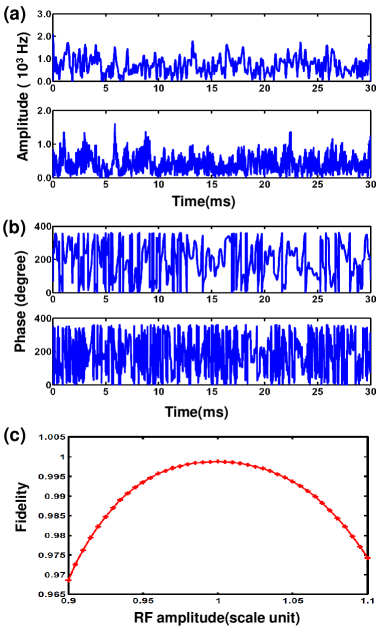
Figure 9: An example of one GRAPE pulse for implementing adiabatic evolution. Time-dependence of the amplitude (a) and the phase (b) of the GRAPE pulse in the ¹³C (top) and ¹⁹F (bottom) channels. (c) Robustness of the GRAPE pulse against RF inhomogeneities.

IV Experimental results and analysis

IV.1 Experimental Spectra

Figure 10 shows the experimental ¹³C spectra for equilibrium state after a reading-out pulse $[\frac{\pi}{2}]_{x}^{{}^{13}C}$ (a), measuring the Wilson-loop operator $\langle\hat{W}(C)\rangle$ (i.e., after the reading-out pulse $[\frac{\pi}{2}]_{x}^{F_{1}}[\frac{\pi}{2}]_{\bar{y}}^{F_{2}}[\frac{\pi}{2}]_{x}^{F_{3}}$) and the single-particle operator $P$ (i.e., decoupling ¹⁹F without a reading-out pulse) on the $M=31$ instantaneous states during the adiabatic passage, respectively. The experimental values of $P$ were directly extracted from the integration of the resonant peak of the ¹⁹F-decoupled ¹³C spectra, while the experimental values of $\langle\hat{W}(C)\rangle$ determined by

$$\langle\hat{W}(C)\rangle=P_{1}-P_{2}-P_{3}-P_{4}+P_{5}+P_{6}+P_{7}-P_{8}$$ (11)

where $P_{i}\,(i=1,2,\cdots,8)$ represents the integration of the $i^{th}$ resonant peak.

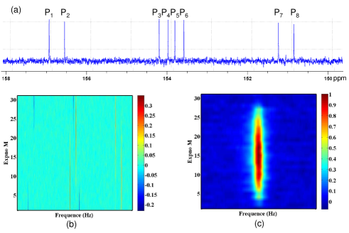
Figure 10: Experimental ¹³C spectra for (a) equilibrium state after a reading-out pulse $[\frac{\pi}{2}]_{x}^{{}^{13}C}$, (b) measuring the Wilson loop operator $\langle\hat{W}(C)\rangle$, and (c) measuring the single-particle operator $P$. (b) and (c) are two-dementional spectra with the total number of experiments $M=31$, and (c) are the ¹⁹F-decoupled ¹³C spectra.

IV.2 State tomography of the ground states

Due to the unlabeled sample, it is difficult to directly measure the ¹⁹F signals related to quantum simulator with the ¹³C nucleus. Thus we transferred the states of the ¹⁹F spins to the ¹³C spin by a SWAP gate and read out the state information of the ¹⁹F spins through the ¹³C spectra. To reconstruct the full density matrices of the four-qubit states, we performed the 44 independent experiments (see Fig. 11) to obtain the coefficients for all of the 256 operators which comprise a complete operator basis of the four-qubit system. In the experiment, this tomography involves 28 local operations and 3 SWAP gates. All of these operations were realized by GRAPE pulses with 400 $\mu s$ for local operations, 9 ms for the SWAP gates between ${}^{13}C$ and $F_{1}$, $F_{2}$ and 30 ms for the SWAP gate between ${}^{13}C$ and $F_{3}$ due to the relatively weak coupling between them. Figure 12 shows some experimental results for the ground states obtained during the adiabatic passage in the experiments.

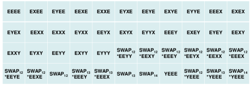
Figure 11: Scheme of the reading-out pulses for the quantum state tomography for our four-qubit quantum simulator. SWAP_ij represents a SWAP gate between spin $i$ and $j$ in order to transfer the ¹⁹F information to ¹³C, and then all signals are obtained from the ¹³C spectra.

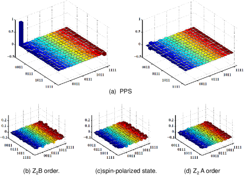
Figure 12: Experimentally reconstructed density matrices. (a) Real (left) and imaginary (right) parts of PPS, with the experimental fidelity around 97.7%. (b)(c)(d) represent the imaginary parts of $Z_{2}B$ order, spin-polarized state and $Z_{2}A$ order, respectively (see Figure 4 in the main text for their real parts).

IV.3 Error Analysis

We calculated the standard deviations $\sigma=\sqrt{\sum_{i=1}^{M}(x_{exp}^{i}-x_{th}^{i})^{2}/M}$ for the experimental measurements of the Wilson loop $\langle\hat{W}(C)\rangle$ and the single-particle properties $P$. The results are listed in Table I. The standard deviations are small and mainly caused by the imperfection of the initial-ground-state preparation, the GRAPE pulses and the others which can be estimated by numerical simulations. Taking the case with $g=1$ as an example, the simulated results are also shown in Table I. Sim1 represents a numerical simulation where we apply the theoretical GRAPE pulses $\hat{U}_{GRAPE}^{th}$ for the adiabatic evolution on the idea initial state $\hat{\rho}_{g}^{th}=|\psi_{g}^{th}\rangle\langle\psi_{g}^{th}|$, i.e., the simulated standard deviations for $\langle\hat{W}(C)\rangle^{sim1}=Tr(\hat{\rho}_{f}^{sim1}\hat{W}(C))$ where $\hat{\rho}_{f}^{sim1}=\hat{U}_{GRAPE}^{th}\hat{\rho}_{g}^{th}\hat{U}_{GRAPE}^{th\dagger}$ and $P^{sim1}=\left|Tr[\hat{\rho}_{f}^{sim1}(\hat{\sigma}^{1}_{x}-i\hat{\sigma}^{1}_{y})]\right|$. This values illustrate the errors only induced by the theoretical imperfection of GRAPE pulses. Sim2 represents a numerical simulation where we apply $\hat{U}_{GRAPE}^{th}$ on the experimentally reconstructed density matrix of the initial state $\hat{\rho}_{g}^{exp}$, i.e., the simulated standard deviations for $\langle\hat{W}(C)\rangle^{sim2}=Tr(\hat{\rho}_{f}^{sim2}\hat{W}(C))$ where $\hat{\rho}_{f}^{sim2}=\hat{U}_{GRAPE}^{th}\hat{\rho}_{g}^{exp}\hat{U}_{GRAPE}^{th\dagger}$ and $P^{sim2}=\left|Tr[\hat{\rho}_{f}^{sim2}(\hat{\sigma}^{1}_{x}-i\hat{\sigma}^{1}_{y})]\right|$. This values account for the errors contributed by the experimental imperfection of preparing initial ground state. The remaining errors can come from the imperfections of experimental quantum control, the static magnetic field and the spectral integrals and so on.

Table 1: The standard deviations of $\langle\hat{W}(C)\rangle$ and P for the experiments and numerical simulations.

	$\sigma_{\langle\hat{W}(C)\rangle}$	$\sigma_{P}$
Exp	0.091	0.078
Sim1	0.043	0.038
Sim2	0.066	0.043

.

References

- (1) S. Sachdev, Quantum Phase Transition (Cambridge University. Press, Cambrige 1999).
- (2) L. D. Landau, Phys. Zs. Sowjet 11, 26 (1937).
- (3) V. L. Ginzburg and L. D. Landau, J. Exp. Eheor. Phys. 20, 1064 (1950).
- (4) D. C. Tsui, H. L. Stormer, and A. C. Gossard, Phys. Rev. Lett. 48, 1559 (1982); R. B. Laughlin, ibid., 50, 1395 (1983).
- (5) X. G. Wen, Int. J. Mod. Phys. B 4, 239 (1990).
- (6) X.-G. Wen and Q. Niu, Phys. Rev. B 41, 9377 (1990).
- (7) D. Arovas, J. R. Schrieffer and F. Wilczek, Phys. Rev. Lett. 53, 722 (1984).
- (8) X. G. Wen, Adv. Phys. 44, 405 (1995).
- (9) A. Kitaev and J. Preskill, Phys. Rev. Lett. 96, 110404 (2006); M. Levin and X. G. Wen, ibid. 96, 110405 (2006).
- (10) A. Kitaev, Ann. Phys. (N.Y.) 303, 2(2003).
- (11) C. Nayak et al., Rev. Mod. Phys. 80,1083 (2008).
- (12) A. Stern and N. H. Lindner, Science 339, 1179-1181 (2013).
- (13) X. G. Wen, Phys. Rev. Lett. 90, 016803 (2003).
- (14) A. Kitaev, Ann. Phys. (N.Y.) 321, 2(2006).
- (15) J. Yu, S. P. Kou, and X. G. Wen, Europhys. Lett. 84, 17004 (2008); S. P. Kou, J. Yu and X. G. Wen, Phys. Rev. B 80, 125101 (2009).
- (16) A. Hamma and D. A. Lidar, Phys. Rev. Lett. 100, 030502 (2008).
- (17) A. Hamma, W. Zhang, S. Haas, and D. A. Lidar, Phys. Rev. B 77, 155111 (2008).
- (18) L. M. Duan, E. Demler, and M. D. Lukin, Phys. Rev. Lett. 91, 090402 (2003); X. J. Liu, K. T. Law, and T. K. Ng, Phys. Rev. Lett. 112, 086401 (2014).
- (19) A. Micheli, G. K. Brennen, and P. A. Zoller, Nat. Phys. 2, 341 (2006).
- (20) J. Q. You, X. F. Shi, X. D. Hu, and F. Nori, Phys. Rev. B 81, 014505 (2010); L. B. Ioffe et al., Nature 415, 503-506 (2002).
- (21) X. C. Yao et al., Nature 482, 489-494 (2012); C. Y. Lu et al., Phys. Rev. Lett. 102, 030502 (2009); J. K. Pachos et al., New. J. Phys. 11, 083010 (2009).
- (22) J. F. Du, J. Zhu, M. G. Hu, and J. L. Chen, arXiv:0712.2694v1 (2007); G. R. Feng, G. L. Long, and R. Laflamme, Phys. Rev. A 88, 022305 (2013).
- (23) X. Chen, Z. C. Gu, X. G. Wen, Phys. Rev. B 82, 155138 (2010)
- (24) R. P. Feynman, Int. J. Theor. Phys. 21, 467 (1982).
- (25) X. H. Peng, J. F. Du, and D. Suter, Phys. Rev. A 71, 012307 (2005); K. Kim et al., Nature 465, 590 (2010); X. H. Peng, J. F. Zhang, J. F. Du and D. Suter, Phys. Rev. Lett. 103, 140501(2009); Gonzalo A. Álvarez and Dieter Suter, Phys. Rev. Lett. 104, 230403 (2010).
- (26) J. F. Du et al., Phys. Rev. Lett. 104, 030502 (2010); B. P. Lanyon et al. Nat. Chem. 2 106 (2010); D. W. Lu et al., Phys. Rev. Lett. 107, 020501 (2011).
- (27) I. M. Georgescu, S. Ashhab and F. Nori, Rev. Mod. Phys. 86, 153 (2014).
- (28) E. Dennis et al., J. Math. Phys. 43, 4452 (2002).
- (29) L. Jiang et al., Nat. Phys. 4, 482-488 (2008).
- (30) X. G. Wen, Phys. Rev. D 68, 065003 (2003).
- (31) See Supplemental Material [url], which includes Refs. Feng2007 ; KouPRL2009 ; Claridge ; Tseng1999 .
- (32) X. Y. Feng, G. M. Zhang, T. Xiang, Phys. Rev. Lett. 98, 087204 (2007).
- (33) S. P. Kou, Phys. Rev. Lett. 102, 120402 (2009).
- (34) Claridge, T. D. W. High resolution NMR techniques in organic chemistry. Tetrahedron Organic Chemistry Series 19 (Elsevier, Amsterdam, 1999).
- (35) C. H. Tseng, et al, Phys. Rev. A 61, 012302 (1999).
- (36) X. Peng et al., Chem. Phys. Lett. 340 (2001).
- (37) N. Khaneja et al., J. Magn. Reson. 172, 296 (2005).
- (38) A. Messiah, Quantum Mechanics (Wiley, New York, 1976).
- (39) J. B. Kogut, Rev. Mod. Phys. 51, 659 (1979).
- (40) J. S. Lee, Phys. Lett. A 305, 349–353(2002)
- (41) W. K. Wootters, Phys. Rev. Lett. 80, 2245 (1998).
- (42) J. Yu and S. P. Kou, Phys. Rev. B 80, 075107 (2009).

References

- (1) X. G. Wen, Phys. Rev. Lett 90, 016803 (2003).
- (2) J. Yu, S. P. Kou, & X. G. Wen, Europhys. Lett., 84, 17004 (2008).
- (3) X. Y. Feng, G. M. Zhang, T. Xiang, Phys. Rev. Lett. 98, 087204 (2007).
- (4) A. Hamma, D. A. Lidar, Phys. Rev. Lett. 100, 030502(2008).
- (5) A. Hamma, W. Zhang, S. Haas, D. A. Lidar, Phys. Rev. B 77, 155111 (2008).
- (6) A. Kitaev, Ann. Phys. 303, 2(2003).
- (7) S. P. Kou, Phys. Rev. Lett. 102, 120402 (2009).
- (8) J. Yu and S. P. Kou, Phys. Rev. B 80, 075107 (2009).
- (9) Claridge, T. D. W. High resolution NMR techniques in organic chemistry. Tetrahedron Organic Chemistry Series 19 (Elsevier, Amsterdam, 1999).
- (10) Messiah, A. Quantum Mechanics (Wiley, New York, 1976).
- (11) C. H. Tseng, et al, Phys. Rev. A 61, 012302 (1999).
- (12) X. H. Peng, J. F. Zhang, J. F. Du and D. Sutter, Phys. Rev. Lett 103, 140501 (2009).
- (13) Khaneja, N., Reiss, T., Kehlet, C., Schulte Herbrüggen, T. & Glaser, S. J., J. Magn. Reson 172, 296 (2005).