Volumes of conditioned bipartite state spaces
Abstract
We analyse the metric properties of conditioned quantum state spaces . These spaces are the convex sets of density matrices that, when partially traced over degrees of freedom, respectively yield the given density matrix . For the case , the volume of equipped with the Hilbert-Schmidt measure is a simple polynomial of the radius of in the Bloch-Ball. Remarkably, the probability to find a separable state in is independent of (except for pure). Both these results are proven analytically for the case of the family of -states, and thoroughly numerically investigated for the general case. The important implications of these results for the clarification of open problems in quantum theory are pointed out and discussed.
pacs:
03.67.-a, 42.50.Dv, 89.70.+cI Introduction
Open quantum system states are reduced system states of some total state of a system and its environment , where denotes the partial trace over the degrees of freedom of the environment. Open quantum system dynamics refers to the time evolution determined through the unitary evolution of system and environment alicki_quantum_1987 : . A crucial issue that is widely discussed (see for example pechukas_reduced_1994 ; alicki_comment_1995 ; pechukas_pechukas_1995 ; rodriguez-rosario_linear_2010 ) is how to map the state of the open system at some initial time to a total state of (formalized through the so-called assignment map ). In the literature this assignment is always considered to be linear and most results are obtained on the assumption that maps on a product with a fixed state of the environment, i.e. .
While the mathematical properties of have been discussed in detail rodriguez-rosario_linear_2010 ; jordan_assumptions_2006 ; masillo_remarks_2011 , only little is known jordan_dynamics_2004 about its image, i.e. the set of total states of the closed system that are compatible with a given reduced state of the open system . A thorough investigation of these spaces is therefore necessary to obtain a more complete picture of the properties of assignment maps, and thus, a more complete picture of open quantum system dynamics.
Apart from their relevance for the description of open quantum dynamics, spaces of total states that are conditioned to a given reduced state constitute lower-dimensional sections of the total state space. An analysis of these sections might hence shed light on the properties of the total space. As only little is known about general quantum dynamical state spaces (see e.g. kimura_bloch_2003 for a discussion of the state space of a qubit and zyczkowski_hilbertschmidt_2003 ; sommers_bures_2003 for the Hilbert-Schmidt and the Bures volume of general state spaces) an investigation of a new kind of sections of these spaces might lead the way to a solution of long-standing problems concerning quantum dynamical state spaces.
In their seminal work zyczkowski_volume_1998 , Życzkowski et al. raised the question of the volume of separable states in the total state space of a bipartite system and emphasized that its solution is of both philosophical and experimental interest. Ever since, this problem has been tackled for different measures both numerically and analytically. Analytical results are at hand only for certain lower-dimensional sections of the total state space slater_exact_2000 . For the general problem only conjectures based on extensive numerical research exist slater_concise_2013 . The conjecture that is of most importance for this paper is the belief that , the a priori Hilbert-Schmidt-probability for a two-qubit state to be separable, is equal to slater_dyson_2007 . In spite of the existence of these analytical and numerical results, a more general geometric picture of state correlations is highly desirable. Our results on conditional state spaces presented here may help to shed light on some long-standing open problems concerning geometrical considerations of state spaces.
Our paper is structured as follows: In section II and III the general framework of bipartite systems is introduced. A possible parametrisation of these systems that will be used throughout this paper, is presented. The state spaces are equipped with the Hilbert-Schmidt measure as the measure for which all metric results will be derived. Section IV introduces coupled qubit systems, which are the lowest-dimensional possible bipartite systems and therefore allow for a feasible numerical treatment. The main results of this paper are to be found in sections V, VI and VII. In the first of these, analytical results for the Hilbert-Schmidt volume of spaces of conditioned -states and the probability to find a separable state in these spaces are derived, while the latter two constitute a numerical investigation of the metric properties of general coupled qubit-systems. A conclusion and a discussion of the implications of the results are given in section VIII.
II State spaces of bipartite quantum systems
An density matrix is a bounded linear operator acting on the Hilbert space (i.e. ) that satisfies the following three conditions:
-
1.
-
2.
-
3.
is positive semi-definite.
The convex set of all density matrices is denoted by . Because of the unit trace and the hermiticity of density matrices, the number of free real parameters of is equal to . The demand for positivity restricts the domain of these parameters.
If is not prime, can be considered as a bipartite state consisting of an -dimensional system coupled to an -dimensional system . A natural parametrisation of an density matrix makes use of the traceless generators of the special unitary group jordan_mapping_2006 (Einstein summation convention implied):
| (1) |
where and are the generators of the groups and , respectively, and is the identity matrix. and are chosen to satisfy the standard orthonormality relations
| (2) |
The parametrisation given by equation (1) is not the only one in use. In the literature parametrisations that use the Cholesky decomposition daboul_conditions_1967 ; slater_radial_2010 or the Euler angles of the elements of the group tilma_generalized_2002 ; byrd_differential_1998 can also be found. Which parametrisation to employ depends strongly on the problem to be solved. In the context of bipartite systems, parametrisation (1) is advantageous, as it directly implements the unity trace and the hermiticity of , and the states and of the systems and can be inferred directly:
| (3) |
where and denote the partial traces over the degrees of freedom of the systems and respectively. In the following, the state will be called the total state, whereas will be called the reduced state of to emphasize the connection with open quantum system dynamics.
The vector completely determines the state and vice versa. The positivity of density matrices restricts the possible vectors to a proper subset of .
In the framework of open system quantum mechanics, so called assignment maps are introduced pechukas_reduced_1994 . These maps assign a compatible total state to each reduced state of the open system. In the language of this article, an assignment map is a map with the property
| (4) |
For a given reduced state , the total state with is obviously not unique. In order to gain a better understanding of open quantum dynamics, it is therefore necessary to investigate the spaces of total states that are conditioned on a given reduced state . These spaces will be denoted as :
| (5) |
Its corresponding subspace of will be denoted as .
Given that
| (6) |
a thorough analysis of conditioned spaces will not only shed light on assignment maps, but also on the properties of the total state space . Before metric properties of can be discussed, it is necessary to introduce the notion of measure in . Then, for example its volume and the a priori probability to find a separable state when choosing a state at random can be determined.
III The Hilbert-Schmidt measure
While the space of pure -dimensional states has a natural measure, the so-called Fubini-Study
measure study_kurzeste_1905 , there is no unique measure to choose in the space of mixed states. As for the parametrisation, the choice of the employed measure depends on the
question that is to be answered. A comprehensive overview over a wide family of measures in
can be found in bengtsson_geometry_2008 .
One possibility to introduce the notion of distance that induces a measure in the space
makes use of the unitarily invariant Hilbert-Schmidt inner product
:
| (7) |
Following this definition, the Hilbert-Schmidt distance of two arbitrary density matrices can be expressed as
| (8) |
The Hilbert-Schmidt distance induces a flat metric in because of the tracelessness of the generators of the group and the orthonormality relations (2):
| (9) |
Up to an insignificant constant (which could be set equal to one by a change of the normalization of (1)), the mapping
| (10) |
is bijective and isometric. Therefore, any metric results about equipped with the Hilbert-Schmidt distance directly give the corresponding metric result in equipped with the flat euclidian metric, and vice versa. This, of course, is also true for any subspaces of and respectively, in particular for the spaces and .
The Hilbert-Schmidt volume of the space has been calculated by Życzkowski and Sommers in zyczkowski_hilbertschmidt_2003 :
| (11) |
where is the Gamma function of . The derivation of (11) makes use of the fact that any density matrix can be represented as , where is a positive diagonal matrix with and is a unitary matrix. As the Hilbert-Schmidt distance is unitarily invariant, its corresponding volume element can be written as a product measure
| (12) |
where is a measure on the space of
positive diagonal -matrices with , i.e. the
-simplex, and is a measure on the space of unitary matrices that is induced by the Haar-measure on . Both these measures can be expressed
analytically and the Hilbert-Schmidt volume of can be calculated
without resorting to the particular parametrisation (1).
For conditioned spaces, the property that the Hilbert-Schmidt measure is of product form fails to
apply. It is still true that any density matrix can be
represented as , but for a given diagonal matrix ,
only certain matrices lead to a density matrix , while most result in a state . The volume of the total space
can be obtained by integrating over the whole space of unitary
matrices 111In fact, the integral in zyczkowski_hilbertschmidt_2003 is not evaluated
over the total group , but merely over the flag manifold . This does however not
change the argument. independently of the entries of the matrix . In the case of
conditioned spaces, however, this independence no longer exists. Therefore, the considerations which
led to
the result (11) cannot be used in order to find the Hilbert-Schmidt
volume of
the conditioned spaces .
While the Hilbert-Schmidt volume of has been calculated, there only
exist conjectures for the a priori probabilities (see
slater_concise_2013 and references therein) and
slater_priori_2003 to find a separable state in
(the state space of two coupled qubits) and
(the state space of a qubit coupled to a qutrit) equipped with the Hilbert-Schmidt measure. As for the calculation of the
volume of conditioned state spaces, the problem of finding general analytical results for
is related to the fact that the Hilbert-Schmidt measure
in the
space of separable states is not of product form. Moreover, there are no unambiguous criteria for
the distinction between separable and entangled states beyond the case
horodecki_separability_1996 ; peres_separability_1996-1 . The same holds of course for
the corresponding a priori probabilities to find a
separable state in the respective conditioned spaces .
The calculation of as well as the investigation of the a
priori probabilities are important in the context of open
quantum dynamics, but they also shed further light on the structure and the properties of the total state
space . As the measures involved are complicated and not explicitly
known, it is unlikely that the techniques used in zyczkowski_hilbertschmidt_2003 and
sommers_bures_2003 can be employed in order to solve these problems. It proves
fruitful, however, to exploit the isometry of the metric spaces and , i. e.
make use of the particular parametrisation (1), in order to find both numerical
results and analytical conjectures for the Hilbert-Schmidt volume of and the a priori probabilities .
IV Coupled qubit-systems
The only quantum dynamical state space whose structure is completely known is the three-dimensional one-qubit state space (see for example kimura_bloch_2003 for a thorough discussion of its properties). Expressed in the parametrisation (1), adapted to a monopartite system, any qubit-state can be written as
| (13) |
where the operators are the well-known Pauli-matrices. The constraint of positive semi-definiteness restricts the so-called Bloch-vector to a solid ball (the Bloch-ball) of radius . The pure qubit-states make up the surface of this ball, the mixed states lie in the interior and the completely mixed state is at the center of the ball.
The lowest-dimensional state-space of a bipartite system is the space ,
i.e. the state space of two coupled qubits. Systems of coupled qubits play an important role in the
context of quantum computation (cf. nielsen_quantum_2000 ) and the dimensions of
and are low enough to allow for
direct calculations in the coordinates of parametrisation (1). Therefore the
following investigations will be mainly restricted to the case.
Any two-qubit-state can be written as
| (14) |
where and are the Pauli-matrices of the qubits, respectively. The reduced state is completely defined by the vector . All further considerations will be simplified by the observation that both the Hilbert-Schmidt measure in the space and the separability of a state are invariant under a transformation , where is an arbitrary special unitary matrix . As the group is the double cover of the group of three-dimensional rotations, taylor_cover_1954 , and only depend on the radius of in the Bloch-ball. Accordingly, it is sufficient to calculate the volume and the probability for a ray from the center of the Bloch-ball to its surface, i.e. . In the following, this ray will be chosen to be the ray from the center of the Bloch-ball to its north-pole, i.e. . As the calculations are too involved to be carried out analytically even for the two-qubit case, they will be conducted in a first step for the seven-dimensional family of two-qubit -states.
V Conditioned volume and a priori Hilbert-Schmidt separability probability for -states
A possible family of states in that allows for analytical conclusions, is the family of -states. These are density matrices of the form
| (15) |
They have been introduced in maziero_classical_2009-1 ; vedral_entanglement_1998 as a
seven-dimensional family of states that contains maximally entangled pure states, as well as
separable states. Because of their simple form, it is possible to carry out various analytical
computations, like for example the calculation of the quantum discord of an
-state ali_quantum_2010 . Note that the definition of -states requires the choice of a
fixed basis. Here, the basis is chosen such that the Bloch-vector of the reduced state has a
-component only (see below). -states do not constitute a ”random” subset of
, but possess an underlying symmetry rau_algebraic_2009 , which
might help to generalise the results found for -states to arbitrary systems.
A comparison of (14) and (15) shows that any -state can be
represented as
| (16) |
As both and are equal to zero, the reduced states of -states lie by construction on the ray from the center of the Bloch-ball to its north pole. The eigenvalues of can be expressed analytically ali_quantum_2010 , and the two eigenvalues that are of importance for the definiteness of lead to the conditions:
| (17) | |||
| (18) |
The inequalities (17) and (18) define two hypersurfaces in that confine the space of -states. The conditioned volume can be calculated by evaluating the integral
| (19) |
and multiplying it by the appropriate factor, i.e. . The explicit calculation is carried out in appendix A. It yields the surprisingly simple result
| (20) |
As a by-product of this formula, the Hilbert-Schmidt volume of the space of -states can be derived:
| (21) |
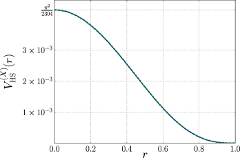
In figure 1 we show the analytical curve from (20) in
comparison with
numerical results obtained from a Monte-Carlo integration.
For the special case of -states, the partial transpose with respect to the second qubit only changes the signs of and . The PPT-criterion (cf. horodecki_separability_1996 ; peres_separability_1996-1 ) for the separability of a state together with inequalities (17) and (18) then allows for a direct calculation of the volume of separable -states, . The ratio determines , the probability to find a separable state in . This calculation is carried out in appendix B. It yields:
| (22) |
We also performed numerical Monte-Carlo calculations which confirmed these values. Most remarkably, the probability to find a separable state in a conditioned state space is independent of the reduced state, i.e. independent of the radius for and jumps to one in a discontinuous way at . The latter fact that is clear: a pure reduced state () can only be realized by a product and thus, a separable total state.
VI Conditioned volume
While the eigenvalues of -states can be easily expressed analytically, the eigenvalues of a
general two-qubit state could, in principle, be calculated. So far, however, a direct derivation of the volume
from these expressions is beyond reach. For higher dimensional
cases, i.e. for a qubit coupled to an -dimensional environment, not even the eigenvalues can be found
analytically. Accordingly, for and
only numerical results are provided here. The knowledge of
and , however, allows for conjectures of the analytical expressions for
and .
The Hilbert-Schmidt volume is numerically estimated by a
Monte-Carlo integration. It can be readily derived that the range of each of the parameters ,
and in the normalization of (14) is . Therefore,
a cube of edge length centred around the origin completely encompasses each conditioned
two-qubit space and its euclidian volume can be estimated by a simple
rejection sampling. Figure 1 shows the accuracy of this procedure for the
six-dimensional case of conditioned -states, where we compare to analytical results.
The full two-qubit problem is -dimensional.
The higher dimension requires a larger number of samples in order to achieve similar accuracy.
For the general case of a qubit coupled to an -dimensional environment, the
enormous number of samples necessary to obtain representative numerical results renders
rejection sampling methods useless.
A sampling method that goes without the rejection of sampling points makes use of the fact that
density matrices can be sampled uniformly distributed according to the Hilbert-Schmidt
measure, by sampling pure -dimensional states uniformly distributed according to the
Fubini-Study measure and partially tracing them over degrees of freedom (cf.
bengtsson_geometry_2008 ). Applied to the case of density matrices, this means
that they can be sampled according to Hilbert-Schmidt measure, by sampling -dimensional pure
states according to the Fubini-Study measure (see e.g. bengtsson_geometry_2008 , chapter ,
for a description of how to sample pure states uniformly distributed according to the Fubini-Study
measure) and partially tracing these states over degrees of freedom. In order to sample states conditioned on a
given qubit state according to
Hilbert-Schmidt measure, it is sufficient to restrict the sampling of the pure states to the subset
of pure states that yield the given qubit state when partially traced over degrees of
freedom. By construction, every sample then gives a valid density matrix, which
increases the accuracy of the results and makes it independent of . This sampling method is hence well suited to
estimate and the course of .
However, it does not yield any estimates of the absolute values of
and, therefore, has to be combined with the results of the rejection sampling.
The result for obtained from a Monte-Carlo integration with
samples is displayed in figure 2.
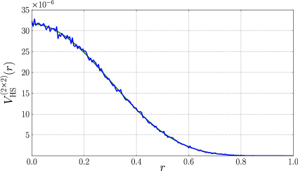
The course of the numerical result resembles the analogous analytical result for . For scaling reasons, the highest power of in an analytical expression for has to be which leads to the conjecture that is given by
| (23) |
The fit of the conjectured curve to the numerical data is shown in figure 2. Assuming that equation (23) is correct, the value of can be calculated by connecting to the volume of the total two-qubit state space:
| (24) |
where the factor is necessary to convert from the euclidean to the Hilbert-Schmidt volume 222Note that equation (24) is not a relation of volumes. is a -dimensional volume, while is a -dimensional one. They cannot be compared in a meaningful way. Therefore (24) is merely an equation to calculate the numerical value of . From (11) it can then be deduced that
| (25) |
This value coincides perfectly with the analogous value found via the Monte-Carlo sampling:
| (26) |
The agreement of the conjectured formula and the numerical results, and the fact that seems to be described by a simple polynomial, suggest the following generalization of (23) for the case:
| (27) |
The corresponding conjecture for follows as in (24):
| (28) |
It is rather difficult to investigate the validity of (27) and
(28) with a numerical procedure that involves the rejection of samples, as the
dimension of the corresponding state spaces grows rapidly and the huge number of required samples to
obtain meaningful results cannot be reached within an acceptable amount of time even for the case
.
However, by employing the method described above (not relying on the rejection of
samples) at least (27) can be verified numerically. This is done by sampling
states
uniformly distributed according to the Hilbert-Schmidt measure, and recording their radius in the
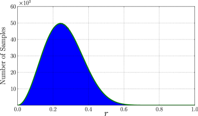
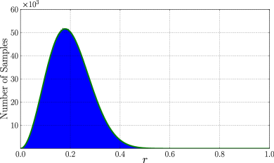
Bloch-ball, respectively. The resulting histogram then has an envelope that is described by a
function proportional to , where
is the conjectured formula (27). It is necessary to multiply by the factor , which is the area of the respective spheres, in order to correctly describe the envelope of
the histograms as they display the number of states sampled for a given radius of the reduced
states. The histograms for the and the case are shown in figure
3. They coincide perfectly with (27).
VII Conditioned a priori Hilbert-Schmidt separability probability
Numerical results for the probability can easily be obtained
with high
accuracy by employing the sampling method that does not require the rejection of
samples. To this end, for each radius , total states with the given radius are sampled, and,
at least for and , the separability of each of these states is checked via the
PPT-criterion. The ratio of the number of separable states to the total number of sampled states
then gives an estimate for .
As it is not the absolute volume of the space of separable states that is to be estimated, but
rather the ratio of the two volumes and
, this sampling procedure in this case does not only give
qualitative
but also quantitative results. For the case they are displayed in figure
4.
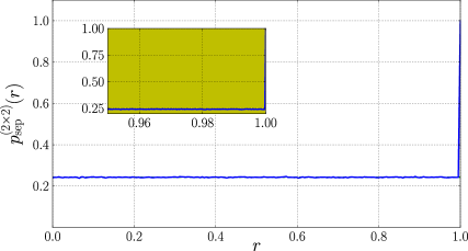
The resemblance to the corresponding results for the -states is striking: our numerical evidence strongly suggests that is constant for and jumps to in a discontinuous way. As for -states it is clear why . The fact that this jump is discontinuous cannot yet be formally proven, but the thorough numerical investigation of the region , also shown in figure 4, strongly suggests this conjecture. Obviously, from a knowledge of , the value of the total state space could be computed to be
| (29) |
The numerical results for obtained above yield
| (30) |
Apart from a postulated but not yet formally proven formula slater_concise_2013 , there do not exist any analytical results for . However, based on extensive numerical research, a value of
| (31) |
has been conjectured (cf. slater_concise_2013 and references therein). The agreement between (30) and (31) further supports the conjecture of this value.
The accuracy of the sample method without rejection even allows for an expansion of the numerical investigation of and the probability to find a state with positive partial trace, . The respective results are shown in figure 5.
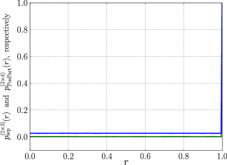
They correspond qualitatively to the according results for . Most remarkably, within numerical confidence, and are independent of – except for the case . For the case a numerical investigation of was conducted by Slater in slater_priori_2003 . It yielded:
| (32) |
From the numerical results above we find that
| (33) |
which is in good correspondence with (32).
The independence of the
functions
, and
of leads to the conjecture that
| (34) |
As beyond the case there is no simple criterion to decide whether or not a bipartite state is separable, it is easier to test the more conservative conjecture
| (35) |
where denotes the a priori Hilbert-Schmidt probability for a state in with a positive partial transpose.
VIII Conclusion and discussion
Although certain lower dimensional sections of the space have already been studied analytically (see e.g. slater_exact_2000 ), not much attention has been given to the conditioned spaces yet. A thorough knowledge of their properties is crucial for the understanding of assignment maps in the framework of open quantum systems and might help to shed light on fundamental open questions in quantum state geometry.
In this work, the metric properties of the conditioned spaces equipped with the Hilbert-Schmidt measure have been investigated numerically and it turned out that the Hilbert-Schmidt volume follows a simple polynomial of the radius in the Bloch sphere of the reduced state , while the probability to find a separable state in a conditioned space is independent of – except for the case . Both these results can be proven analytically for the case of the seven-dimensional family of -states.
Above all, the independence of of the radius we found is intriguing, as it, once analytically proven, opens new ways to study properties of the total state space through these conditional cuts.
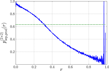
It is important to point out that all these results and conjectures
only hold for the Hilbert-Schmidt measure. This particularity further singles out this measure
amongst all other unitarily invariant measures. The corresponding results for the example of the
product measure used in zyczkowski_volume_1998 are shown in figure
6.
One mean to find analytical expressions for all quantities investigated in this paper could be
the use of -states. Obviously, there is a deep qualitative connection between the metric
properties of this seven-dimensional family of states, and the corresponding total space of states.
A thorough investigation of higher-dimensional -states, i.e. in a first step
-states, might therefore further support the conjectures made for the general space
. Furthermore, they might even be helpful from a quantitative point of
view. While the conjectured value for of
seems
plausible, the origins of this simple fraction still remain unclear.
From formula (47) the volume of conditioned entangled -states can be derived to be equal to . If denotes the number of free parameters for conditioned -states, the denominator
is equal to . If denotes the corresponding number for
the full problem, it can easily be seen that the denominator of the conjectured value of
is equal to . While this
is still
highly speculative, it nevertheless suggests that the analytical results for -states might be
generalisable to the total and even higher-dimensional cases.
Acknowledgments
It is a pleasure to thank Karol Życzkowski for fruitful discussions and helpful advice.
Appendix A Volume of the space
Semi-definiteness of yields two inequalities that define the seven-dimensional subspace occupied by X-states in the full two-qubit parameter space:
| (36) | |||
| (37) |
(36) and (37) set the limits for : . Given these limits, (36) and (37) can be squared, and one obtains:
| (38) | |||
| (39) |
The task of calculating the volume defined by these two inequalities is remarkably simplified by the following coordinate transformation:
This transformation is singular for . However, for this value of the space is lower-dimensional, and its volume therefore zero. The Jacobian of this transformation is and in the new coordinates (38) and (39) read as:
| (40) | |||||
| (41) |
with
From (40) and (41) it follows that the integrals in the -plane and the -plane will merely give the areas of circles of radius and , respectively. As both and have to be positive, and range from to . The euclidian volume of the space of conditioned -states can then be calculated:
| (42) | |||||
which is valid for all . From (42), the result (20) for follows directly.
Appendix B A priori probability to find a separable state in
In order for a two-qubit-state to be separable, its partial transpose with respect to one of the subsystems has to be positive semi-definite horodecki_separability_1996 ; peres_separability_1996-1 . For the special case of -states, the partial transpose with respect to the second qubit merely changes the signs of and . An -state is hence separable iff it satisfies the two additional restrictions
| (43) | |||||
| (44) |
Together with (40) and (41), these two inequalities allow for a direct calculation of , the euclidian volume of separable -states:
| (45) |
where denotes the minimum of . A short calculation yields that
and therefore
| (46) |
It is easy to verify that (46) leads to the result
| (47) |
Accordingly, for , the probability is independent of and equal to:
For all reduced states are pure, and therefore all the corresponding total states are separable. Hence: .
References
- (1) In fact, the integral in zyczkowski_hilbertschmidt_2003 is not evaluated over the total group , but merely over the flag manifold . This does however not change the argument.
- (2) Note that equation (24) is not a relation of volumes. is a -dimensional volume, while is a -dimensional one. They cannot be compared in a meaningful way. Therefore (24) is merely an equation to calculate the numerical value of .
- (3) Mazhar Ali, A. R. P. Rau, and G. Alber. Quantum discord for two-qubit x states. Physical Review A, 81(4):042105, April 2010.
- (4) R. Alicki and K. Lendi. Quantum dynamical semigroups and applications. Springer, 1987.
- (5) Robert Alicki. Comment on ”Reduced dynamics need not be completely positive”. Physical Review Letters, 75(16):3020–3020, October 1995.
- (6) Ingemar Bengtsson and Karol Życzkowski. Geometry of quantum states: an introduction to quantum entanglement. Cambridge University Press, 2008.
- (7) Mark Byrd. Differential geometry on SU(3) with applications to three state systems. Journal of Mathematical Physics, 39(11):6125–6136, November 1998.
- (8) J. Daboul. Conditions on density matrix elements and their application in resonance production. Nuclear Physics B, 4(1):180–188, December 1967.
- (9) Michał Horodecki, Paweł Horodecki, and Ryszard Horodecki. Separability of mixed states: necessary and sufficient conditions. Physics Letters A, 223(1–2):1–8, November 1996.
- (10) Thomas F. Jordan. Assumptions that imply quantum dynamics is linear. Physical Review A, 73(2):022101, February 2006.
- (11) Thomas F. Jordan, Anil Shaji, and E. C. G. Sudarshan. Dynamics of initially entangled open quantum systems. Physical Review A, 70(5):052110, November 2004.
- (12) Thomas F. Jordan, Anil Shaji, and E. C. G. Sudarshan. Mapping the schrödinger picture of open quantum dynamics. Physical Review A, 73(1):012106, January 2006.
- (13) Gen Kimura. The bloch vector for n-level systems. Physics Letters A, 314(5–6):339–349, August 2003.
- (14) F. Masillo, G. Scolarici, and L. Solombrino. Some remarks on assignment maps. Journal of Mathematical Physics, 52(1):012101, January 2011.
- (15) J. Maziero, L. C. Céleri, R. M. Serra, and V. Vedral. Classical and quantum correlations under decoherence. Physical Review A, 80(4):044102, October 2009.
- (16) Michael A Nielsen and Isaac L Chuang. Quantum computation and quantum information. Cambridge University Press, 2000.
- (17) Philip Pechukas. Reduced dynamics need not be completely positive. Physical Review Letters, 73(8):1060–1062, August 1994.
- (18) Philip Pechukas. Pechukas replies:. Physical Review Letters, 75(16):3021–3021, October 1995.
- (19) Asher Peres. Separability criterion for density matrices. Physical Review Letters, 77(8):1413–1415, August 1996.
- (20) A. R. P. Rau. Algebraic characterization of x-states in quantum information. Journal of Physics A: Mathematical and Theoretical, 42(41):412002, October 2009.
- (21) César A. Rodríguez-Rosario, Kavan Modi, and Alán Aspuru-Guzik. Linear assignment maps for correlated system-environment states. Physical Review A, 81(1):012313, January 2010.
- (22) Paul B Slater. Exact bures probabilities that two quantum bits are classically correlated. The European Physical Journal B-Condensed Matter and Complex Systems, 17(3):471–480, 2000.
- (23) Paul B. Slater. A priori probability that a qubit-qutrit pair is separable. Journal of Optics B: Quantum and Semiclassical Optics, 5(6):651–656, December 2003. arXiv:quant-ph/0211150.
- (24) Paul B. Slater. Dyson indices and Hilbert–Schmidt separability functions and probabilities. Journal of Physics A: Mathematical and Theoretical, 40(47):14279, November 2007.
- (25) Paul B. Slater. Radial and azimuthal profiles of two-Qubit/Rebit hilbert-schmidt separability probabilities and related 3-d visualization analyses. arXiv:1010.5180 [math-ph, physics:quant-ph], October 2010.
- (26) Paul B. Slater. A concise formula for generalized two-qubit Hilbert–Schmidt separability probabilities. Journal of Physics A: Mathematical and Theoretical, 46(44):445302, November 2013.
- (27) Hans-Jürgen Sommers and Karol Życzkowski. Bures volume of the set of mixed quantum states. Journal of Physics A: Mathematical and General, 36(39):10083–10100, October 2003.
- (28) E. Study. Kürzeste Wege im komplexen Gebiet. Mathematische Annalen, 60(3):321–378, September 1905.
- (29) R. L. Taylor. Covering groups of nonconnected topological groups. Proceedings of the American Mathematical Society, 5:753–768, 1954.
- (30) Todd Tilma and E. C. G. Sudarshan. Generalized euler angle parametrization for SU(N). Journal of Physics A: Mathematical and General, 35(48):10467, December 2002.
- (31) V. Vedral and M. B. Plenio. Entanglement measures and purification procedures. Physical Review A, 57(3):1619–1633, March 1998.
- (32) Karol Życzkowski, Paweł Horodecki, Anna Sanpera, and Maciej Lewenstein. Volume of the set of separable states. Physical Review A, 58(2):883–892, August 1998.
- (33) Karol Życzkowski and Hans-Jürgen Sommers. Hilbert–Schmidt volume of the set of mixed quantum states. Journal of Physics A: Mathematical and General, 36(39):10115, October 2003.