Physical Formulation and Numerical Algorithm
for Simulating N Immiscible Incompressible Fluids Involving General Order Parameters

Abstract

We present a physical formulation, and a numerical algorithm, based on a class of general order parameters for simulating the motion of a mixture of $N$ ($N\geqslant 2$) immiscible incompressible fluids with given densities, dynamic viscosities, and pairwise surface tensions. The introduction of general order parameters leads to a more strongly coupled system of phase field equations, in contrast to that with certain special choice of the order parameters. However, the general form enables one to compute the N-phase mixing energy density coefficients in an explicit fashion in terms of the pairwise surface tensions. From the simulation perspective, the increased complexity in the form of the phase field equations with general order parameters in actuality does not induce essential computational difficulties. Our numerical algorithm reformulates the ($N-1$) strongly-coupled phase field equations for general order parameters into $2(N-1)$ Helmholtz-type equations that are completely de-coupled from one another, leading to a computational complexity essentially the same as that of the simpler phase field equations associated with special choice of order parameters. We demonstrate the capabilities of the method developed herein using several test problems involving multiple fluid phases and large contrasts in densities and viscosities among the multitude of fluids. In particular, by comparing simulation results with the Langmuir-de Gennes theory of floating liquid lenses we show that the method produces physically accurate results for multiple fluid phases.

Keywords: N-phase flow; general order parameters; pairwise surface tensions; large density contrast; phase field; multiphase flow

1 Introduction

The present work focuses on the motion of a mixture of $N$ ($N\geqslant 2$) immiscible incompressible fluids with given densities, dynamic viscosities, and pairwise surface tensions. The system is assumed to contain no solid phase (e.g. solid particles), except for possible solid-wall boundaries. The situation is a generalization of incompressible two-phase flows, which have been under intensive investigations by the community for decades. The applications and potential implications of N-phase problems are enormous, from both the practical engineering perspective and fundamental physics perspective Taylor1934 ; deGennesBQ2003 ; SayeS2011 .

N-phase flows have been the subject of a number of past research efforts in the literature. A summary of the existing studies is provided in the following paragraphs. Several researchers have reviewed two-phase flows comprehensively for different approaches and techniques OsherS1988 ; UnverdiT1992 ; AndersonMW1998 ; LowengrubT1998 ; Jacqmin1999 ; ScardovelliZ1999 ; Tryggvasonetal2001 ; SethianS2003 ; see also the references therein. We will therefore restrict our attention in the following review, and also in the main work of the present paper, to flows with three or more fluid phases ($N\geqslant 3$), noting that the technique developed herein equally applies to two-phase flows. It should also be noted that our attention is limited to incompressible fluids.

Since the overall approach of the current work pertains to the phase field framework, we will first briefly mention the representative works for multiple phases based on other related approaches such as level set or volume of fluids, and then will concentrate on the existing studies with phase fields. The level set technique as proposed by OsherS1988 is extended from two to N components in several studies (see e.g. MerrimanBO1994 ; ZhaoCMO1996 ; SmithSC2002 ; ZlotnikD2009 ; VillaF2010 , among others), where different fluid components are differentiated by using $N$ MerrimanBO1994 ; ZhaoCMO1996 , ($N-1$) SmithSC2002 ; ZlotnikD2009 , or $\left\lceil\log_{2}^{N}\right\rceil$ ChanV2001 level set functions. In SayeS2011 the multiple phases are characterized by a single unsigned level set function, and the $\epsilon$ ($\epsilon>0$ is a small number) level sets are convected in the usual way by the flow, while the fluid interfaces at the new step are re-constructed from the $\epsilon$ level sets by a Voronoi tessellation. The work of BonhommeMDP2012 combines the experiments and numerical simulations based on a volume-of-fluid approach, and investigates in detail the dynamics of an air bubble crossing an interface between two fluids.

Let us now concentrate on the past studies of N-phase flows with the phase field (or diffuse interface) approach, which appears to constitute the majority of efforts in this area. The main developments are primarily thanks to the contributions of Kim and collaborators KimL2005 ; Kim2009 ; Kim2012 , Boyer and collaborators BoyerL2006 ; BoyerLMPQ2010 ; BoyerM2011 , and Heida and collaborators HeidaMR2012 . Among these, several investigations have been devoted to the discretizations of the three-component KimKL2004 ; BoyerM2011 or N-component LeeK2008 ; LeeK2012 Cahn-Hilliard equations or Allen-Cahn equations, where the hydrodynamic interaction is absent. In particular, energy-stable schemes for the three-component Cahn-Hilliard equations are discussed in BoyerM2011 , and a nonlinear multigrid method combined with a finite-difference discretization is presented in KimKL2004 ; LeeK2008 . When the hydrodynamic interaction is present, in KimL2005 a thermodynamically-consistent phase field model for N fluid components is derived based on the balance equations and the second law of thermodynamics. This is a generalization of the two-phase model proposed by LowengrubT1998 . An important feature is that, the mixture velocity in this N-phase model is the mass-averaged velocity and therefore it is not divergence free. In BoyerL2006 a three-component Cahn-Hilliard system is coupled with the Navier-Stokes equation, supplemented by a capillary force, to model three-phase flows. The effects of different forms for the bulk free energy have been studied. Noting a solvability difficulty in determining the coefficients for the surface-tension forces when more than three phases are involved, Kim Kim2009 proposed a phenomenological surface-tension force for multiple fluid components; see its applications in Kim2012 ; LeeK2013 . In BoyerLMPQ2010 a combined Cahn-Hilliard/Navier-Stokes model has been studied for three-phase flows, in which the Cahn-Hilliard model uses a particular free-energy form due to BoyerL2006 and the Navier-Stokes equation uses a special form for the inertia term due to GuermondQ2000 . More recently, Heida et al HeidaMR2012 present a Cahn-Hilliard-Navier-Stokes type phase field model for N fluid phases in which the constitutive relations are obtained by requiring the maximization of the rate of entropy production. The mixture velocity in this model, similar to that of KimL2005 ; LiW2014 , is also the mass-averaged velocity and is not divergence free. Another interesting work is MatsutaniNS2011 , in which an Euler type equation, i.e. barring the dissipation terms, with the surface tensions of an N-phase field has been derived based on the variational principle.

Very recently, by considering the mass conservations of the N individual fluid phases, the momentum conservation, Galilean invariance and the second law of thermodynamics, we have derived in Dong2014 a general phase field model (isothermal) for the mixture of N ($N\geqslant 2$) immiscible incompressible fluids; see also Section 1.1 below. This model is fundamentally different from those of KimL2005 ; HeidaMR2012 ; LiW2014 , in that the mixture velocity in our model is the volume-averaged velocity, which can be rigorously shown to be divergence free Dong2014 . In contrast, the velocity in the models of KimL2005 ; HeidaMR2012 ; LiW2014 is the mass-averaged velocity, and is not divergence free. Our N-phase model can be considered as a generalization of the formulation in AbelsGG2012 for two-phase flows.

In order to provide an N-phase formulation suitable for numerical simulations, the general N-phase model of Dong2014 requires the further specification of two items: (1) a set of ($N-1$) order parameters or phase field variables, and (2) the form of the N-phase free energy density function. In Dong2014 we have employed a very special set of order parameters, which is also given in Section 2.1, because this set significantly simplifies the form of the resulting phase field equations. Employing this particular phase field formulation, we have further developed a method for computing the mixing energy density coefficients (see Section 2.1 for definition) involved in the formulation by solving a linear algebraic system based on the pairwise surface tensions among the N fluids. We have also developed an algorithm for solving the coupled system of governing equations in this formulation for N-phase simulations.

In this paper we generalize the N-phase formulation to a class of general order parameters. This gives rise to a class of N-phase physical formulations suitable for numerical simulations. Within this family, by specifying a constant non-singular matrix and a constant vector, one will arrive at a specific N-phase formulation. This class of physical formulations with general order parameters includes the one of Dong2014 as a particular case.

The introduction of the class of general order parameters has two major implications:

• It enables us to derive an explicit expression for the mixing energy density coefficients in terms of the pairwise surface tensions. Therefore, the mixing energy density coefficients with general order parameters can be explicitly computed. In contrast, the method of Dong2014 requires one to solve a linear algebraic system to determine the mixing energy density coefficients.

• The resulting phase field equations have a more complicated form than that employing the special set of order parameters of Dong2014 . In particular, the ($N-1$) phase field equations with general order parameters become much more strongly coupled with one another. The increased complexity raises new challenges to their numerical solutions.

We have developed an algorithm for solving the new phase field equations with general order parameters, which overcomes the computational challenge caused by the increased complexity. Our algorithm reformulates the ($N-1$) strongly-coupled phase field equations for general order parameters into $2(N-1)$ Helmholtz type equations that are completely de-coupled from one another. With this algorithm the computational complexity for the general order parameters is comparable to that of Dong2014 for the simplified phase field equations with the special set of order parameters. This algorithm for the phase field equations with general order parameters, combined with an algorithm for the N-phase momentum equations, provides an efficient method for simulating N-phase flows, which has also overcome the computational issues associated with variable mixture density and viscosity.

The current work is in line with the following view toward the order parameters (or phase field variables). The order parameters or phase field variables serve merely as a set of state variables chosen to formulate the system, and they can be chosen in different ways. Using a different set of order parameters leads to a different representation of the N-phase system. While the resulting phase field equations may have varying degrees of complexity with different order parameters, the various representations of the N-phase system should be equivalent to one another.

The novelties of this paper lie in three aspects: (1) the N-phase physical formulation with general order parameters, (2) the explicit form of the N-phase mixing energy density coefficients in terms of the pairwise surface tensions for general order parameters, and (3) the numerical algorithm for solving the ($N-1$) strongly-coupled phase field equations with general order parameters. In addition, the algorithm for solving the N-phase momentum equations in the current paper, given in the Appendix B, is also new in the context of N-phase flows. Note that it is different than that of Dong2014 for the N-phase momentum equations. But the essential strategies for dealing with the variable density, variable viscosity and the pressure-velocity coupling stem from our previous work DongS2012 for two-phase flows.

The rest of this paper is organized as follows. In Section 1.1 we provide a summary of the general phase field model for a mixture of N immiscible incompressible fluids we derived in Dong2014 , which serves as the basis for the N-phase physical formulations with general order parameters of the current paper. In Section 2 we discuss a class of general order parameters and the N-phase formulations with the general order parameters. We also derive an explicit form for the mixing energy density coefficients in terms of the pairwise surface tensions among the N fluids. Section 3 provides an efficient algorithm for solving the ($N-1$) strongly-coupled phase field equations with general order parameters. We further combine this algorithm, with a scheme for the N-phase momentum equations discussed in Appendix B, to form an overall method for N-phase flow simulations. In Section 4 we look into several numerical examples involving three and four fluid phases to demonstrate the accuracies and capabilities of the presented method with general order parameters. Section 5 concludes the discussions with a summary of the key points. Finally, Appendix A provides a proof for the unique solvability of the linear algebraic system about the mixing energy density coefficients derived in Dong2014 . The unique solvability of this system is an un-settled issue of Dong2014 . Appendix B presents a scheme for the N-phase momentum equations, exploiting the ideas for treating the variable density and variable viscosity in DongS2012 originally developed for two-phase flows.

1.1 A General Phase-Field Model for an N-Fluid Mixture

This subsection summarizes the general phase field model we derived in Dong2014 based on the conservations of mass and momentum, the second law of thermodynamics, and Galilean invariance. We refer to Dong2014 for detailed derivations of this system.

Let $\Omega$ denote the flow domain in two or three dimensions, and $\partial\Omega$ denote the boundary of $\Omega$. consider the mixture of $N$ ($N\geqslant 2$) immiscible incompressible fluids contained in $\Omega$. Let $\tilde{\rho}_{i}$ ($1\leqslant i\leqslant N$) denote the constant densities of these $N$ pure fluids (before mixing), and $\tilde{\mu}_{i}$ ($1\leqslant i\leqslant N$) denote their constant dynamic viscosities. We define the auxiliary parameters

$$\tilde{\gamma}_{i}=\frac{1}{\tilde{\rho}_{i}}\ \text{for}\ 1\leqslant i\leqslant N,\qquad\Gamma=\sum_{i=1}^{N}\tilde{\gamma}_{i},\qquad\Gamma_{\mu}=\sum_{i=1}^{N}\tilde{\gamma}_{i}\tilde{\mu}_{i}.$$ (1)

Let $\phi_{i}$ ($1\leqslant i\leqslant N-1$) denote the ($N-1$) independent order parameters (or interchangeably, phase field variables) that characterize the N-phase system, and $\vec{\phi}=(\phi_{1},\dots,\phi_{N-1})$ denote the vector of phase field variables. Let $\rho_{i}(\vec{\phi})$ and $c_{i}(\vec{\phi})$ ($1\leqslant i\leqslant N$) respectively denote the density and the volume fraction of the $i$-th fluid within the mixture. Let $\rho(\vec{\phi})$ denote the mixture density. We have the relations

$$c_{i}=\frac{\rho_{i}}{\tilde{\rho}_{i}}=\tilde{\gamma}_{i}\rho_{i},\quad\sum_{i=1}^{N}c_{i}=1,\quad\rho=\sum_{i=1}^{N}\rho_{i}.$$ (2)

Let $W(\vec{\phi},\nabla\vec{\phi})$ denote the free energy density function of the system, which must satisfy the following condition

$$\sum_{i=1}^{N-1}\nabla\phi_{i}\otimes\frac{\partial W}{\partial(\nabla\phi_{i})}=\sum_{i=1}^{N-1}\frac{\partial W}{\partial(\nabla\phi_{i})}\otimes\nabla\phi_{i},$$ (3)

where $\otimes$ denotes the tensor product. Then this N-phase system is described by the following equations Dong2014 :

$$\rho\left(\frac{\partial\mathbf{u}}{\partial t}+\mathbf{u}\cdot\nabla\mathbf{u}\right)+\tilde{\mathbf{J}}\cdot\nabla\mathbf{u}=-\nabla p+\nabla\cdot\left[\mu(\vec{\phi})\mathbf{D}(\mathbf{u})\right]-\sum_{i=1}^{N-1}\nabla\cdot\left(\nabla\phi_{i}\otimes\frac{\partial W}{\partial(\nabla\phi_{i})}\right),$$ (4a)

$$\nabla\cdot\mathbf{u}=0,$$ (4b)

$$\sum_{j=1}^{N-1}\frac{\partial\varphi_{i}}{\partial\phi_{j}}\left(\frac{\partial\phi_{j}}{\partial t}+\mathbf{u}\cdot\nabla\phi_{j}\right)=\nabla\cdot\left[\tilde{m}_{i}(\vec{\phi})\nabla C_{i}\right],\qquad 1\leqslant i\leqslant N-1,$$ (4c)

where $\mathbf{u}(\mathbf{x},t)$ is velocity, $p(\mathbf{x},t)$ is pressure, $\mathbf{D}(\mathbf{u})=\nabla\mathbf{u}+\nabla\mathbf{u}^{T}$ (superscript $T$ denoting transpose), $\mathbf{x}$ and $t$ are respectively the spatial and temporal coordinates. $\tilde{m}_{i}(\vec{\phi})\geqslant 0$ ($1\leqslant i\leqslant N-1$) are the mobilities associated with $\phi_{i}$. $\varphi_{i}(\vec{\phi})$ are defined by

$$\varphi_{i}(\vec{\phi})=\rho_{i}(\vec{\phi})-\rho_{N}(\vec{\phi}),\quad 1\leqslant i\leqslant N-1.$$ (5)

The chemical potentials $C_{i}(\vec{\phi},\nabla\vec{\phi})$ ($1\leqslant i\leqslant N-1$) are given by the following linear algebraic system

$$\sum_{j=1}^{N-1}\frac{\partial\varphi_{j}}{\partial\phi_{i}}C_{j}=\frac{\partial W}{\partial\phi_{i}}-\nabla\cdot\frac{\partial W}{\partial(\nabla\phi_{i})},\quad 1\leqslant i\leqslant N-1,$$ (6)

which can be solved once $W(\vec{\phi},\nabla\vec{\phi})$ and $\varphi_{i}(\vec{\phi})$ are given. $\tilde{\mathbf{J}}(\vec{\phi},\nabla\vec{\phi})$ is given by

$$\tilde{\mathbf{J}}=-\sum_{i=1}^{N-1}\left(1-\frac{N}{\Gamma}\tilde{\gamma}_{i}\right)\tilde{m}_{i}(\vec{\phi})\nabla C_{i}.$$ (7)

The mixture density $\rho(\vec{\phi})$ and dynamic viscosity $\mu(\vec{\phi})$ are given by

$$\rho(\vec{\phi})=\frac{N}{\Gamma}+\sum_{i=1}^{N-1}\left(1-\frac{N}{\Gamma}\tilde{\gamma}_{i}\right)\varphi_{i}(\vec{\phi}),\qquad\mu(\vec{\phi})=\frac{\Gamma_{\mu}}{\Gamma}+\sum_{i=1}^{N-1}\left(\tilde{\mu}_{i}-\frac{\Gamma_{\mu}}{\Gamma}\right)\tilde{\gamma}_{i}\varphi_{i}(\vec{\phi}).$$ (8)

2 Order Parameters and N-Phase Physical Formulation

2.1 N-Phase Formulations with General Order Parameters

We consider the mixture of $N$ ($N\geqslant 2$) immiscible incompressible fluids contained in a flow domain $\Omega$ in two or three dimensions. The domain boundary is denoted by $\partial\Omega$. Let $\tilde{\rho}_{i}$ ($1\leqslant i\leqslant N$) denote the constant densities of these $N$ pure fluids (before mixing), and $\tilde{\mu}_{i}$ ($1\leqslant i\leqslant N$) denote their constant dynamic viscosities. Let $\phi_{i}$ denote the ($N-1$) independent order parameters (or interchangeably, phase field variables) that characterize the N-phase system, and $\vec{\phi}=(\phi_{1},\dots,\phi_{N-1})$ denote the vector of phase field variables. Let $\rho_{i}(\vec{\phi})$ ($1\leqslant i\leqslant N$) denote the density of the $i$-th fluid within the mixture. Note that $\rho_{i}$ are field variables.

To arrive at an N-phase physical formulation suitable for numerical simulations, the phase field model given in Section 1.1 requires the specification of: (1) the form of the free energy density function $W(\vec{\phi},\nabla\vec{\phi})$, and (2) the set of order parameters $\phi_{i}$ ($1\leqslant i\leqslant N-1$).

Following Dong2014 , we assume the following form for the free energy density function of the N-phase system

$$W(\vec{\phi},\nabla\vec{\phi})=\sum_{i,j=1}^{N-1}\frac{\lambda_{ij}}{2}\nabla\phi_{i}\cdot\nabla\phi_{j}+\frac{\beta^{2}}{2\eta^{2}}H(\vec{\phi}),\qquad H(\vec{\phi})=\sum_{k=1}^{N}c_{k}^{2}(1-c_{k})^{2},$$ (9)

where $\beta^{2}$ is a characteristic scale for the energy, and $\eta$ is a characteristic scale for the interfacial thickness. $c_{k}(\vec{\phi})$ ($1\leqslant k\leqslant N$) is the volume fraction of the fluid $k$ in the mixture, whose specific form is given subsequently. $\lambda_{ij}$ ($1\leqslant i,j\leqslant N-1$) are referred to as the mixing energy density coefficients, and they are assumed to be constant in the current paper. The condition (3) requires that the matrix

$$\mathbf{A}=\begin{bmatrix}\lambda_{ij}\end{bmatrix}_{(N-1)\times(N-1)}$$ (10)

be symmetric. We further require that $\mathbf{A}$ be positive definite to ensure the positivity of the first term in the $W(\vec{\phi},\nabla\vec{\phi})$ expression. Therefore, the matrix $\mathbf{A}$ is required to be symmetric positive definite (SPD) in the current paper.

The form of the free energy density function (9), in particular the cross terms $\nabla\phi_{i}\cdot\nabla\phi_{j}$ ($i\neq j$) therein, give rise to a set of phase-field equations that are very different from those of the existing N-phase studies KimL2005 ; BoyerL2006 ; Kim2009 ; BoyerLMPQ2010 ; Kim2012 ; LeeK2013 . It is the key that enables us to determine the mixing energy density coefficients $\lambda_{ij}$ uniquely, and to provide their explicit expressions, based on the pairwise surface tensions among the $N$ fluids. This will be discussed subsequently in Section 2.2.

We now focus on the order parameters $\vec{\phi}$, and this is the departure point of the current work. Let

$$\mathbf{A}_{1}=\begin{bmatrix}a_{ij}\end{bmatrix}_{(N-1)\times(N-1)},\qquad\mathbf{b}_{1}=\begin{bmatrix}b_{i}\end{bmatrix}_{(N-1)\times 1}$$ (11)

respectively denote a prescribed non-singular constant matrix and a prescribed constant vector. We define the ($N-1$) order parameters $\phi_{i}$ as follows,

$$\varphi_{i}(\vec{\phi})=\rho_{i}(\vec{\phi})-\rho_{N}(\vec{\phi})=\sum_{j=1}^{N-1}a_{ij}\phi_{j}+b_{i},\qquad 1\leqslant i\leqslant N-1.$$ (12)

Note that $\phi_{i}$ ($1\leqslant i\leqslant N-1$) as defined above can in general be dimensional or non-dimensional variables. However, in the current paper we will require that $\phi_{i}$ be non-dimensional in the simulations. Equation (12) defines a family of order parameters. Given a specific set of $\mathbf{A}_{1}$ and $\mathbf{b}_{1}$ in (11), equation (12) will define a unique set of order parameters $\phi_{i}$ ($1\leqslant i\leqslant N-1$). We refer to the family of order parameters defined by (12) as the general order parameters.

With the set of general order parameters given by (12), and the free energy density function given by (9), the motion of the N-phase mixture is described by the following system of equations,

$$\rho(\vec{\phi})\left(\frac{\partial\mathbf{u}}{\partial t}+\mathbf{u}\cdot\nabla\mathbf{u}\right)+\tilde{\mathbf{J}}(\vec{\phi},\nabla\vec{\phi})\cdot\nabla\mathbf{u}=-\nabla p+\nabla\cdot\left[\mu(\vec{\phi})\mathbf{D}(\mathbf{u})\right]-\sum_{i,j=1}^{N-1}\nabla\cdot\left(\lambda_{ij}\nabla\phi_{i}\nabla\phi_{j}\right)+\mathbf{f}$$ (13a)

$$\nabla\cdot\mathbf{u}=0$$ (13b)

$$\sum_{j=1}^{N-1}d_{ij}\left(\frac{\partial\phi_{j}}{\partial t}+\mathbf{u}\cdot\nabla\phi_{j}\right)=\nabla^{2}\left[-\sum_{j=1}^{N-1}\lambda_{ij}\nabla^{2}\phi_{j}+h_{i}(\vec{\phi})\right]+g_{i}(\mathbf{x},t),\qquad 1\leqslant i\leqslant N-1,$$ (13c)

where we have taken into account an external body force $\mathbf{f}(\mathbf{x},t)$ in the momentum equation (13a), and included a prescribed source term $g_{i}$ in the phase field equations (13c). $g_{i}$ ($1\leqslant i\leqslant N-1$) are for the purpose of numerical testing only, and will be set to $g_{i}=0$ in actual simulations. The constants $d_{ij}$ ($1\leqslant i,j\leqslant N-1$) are defined by

$$\left\{\begin{split}&\mathbf{A}_{2}=\begin{bmatrix}d_{ij}\end{bmatrix}_{(N-1)\times(N-1)}=\mathbf{A}_{1}^{T}\mathbf{M}^{-1}\mathbf{A}_{1},\\ &\mathbf{M}=\text{diag}\left(m_{1}\left(\frac{\tilde{\rho}_{1}+\tilde{\rho}_{N}}{2}\right)^{2},m_{2}\left(\frac{\tilde{\rho}_{2}+\tilde{\rho}_{N}}{2}\right)^{2},\dots,m_{N-1}\left(\frac{\tilde{\rho}_{N-1}+\tilde{\rho}_{N}}{2}\right)^{2}\right),\end{split}\right.$$ (14)

where $m_{i}>0$ ($1\leqslant i\leqslant N-1$) are the interfacial mobility coefficients associated with $\phi_{i}$ and are assumed to be positive constants. Note that the matrix $\mathbf{A}_{2}$ is symmetric positive definite (SPD) based on the assumptions about the non-singularity of $\mathbf{A}_{1}$ and the positivity of $m_{i}$.

The function $h_{i}(\vec{\phi})$ in (13c) is given by

$$h_{i}(\vec{\phi})=\frac{\beta^{2}}{2\eta^{2}}\frac{\partial H}{\partial\phi_{i}},\qquad 1\leqslant i\leqslant N-1,$$ (15)

where $H(\vec{\phi})$ is defined in (9). The volume fractions $c_{k}(\vec{\phi})$ ($1\leqslant k\leqslant N$) with the general order parameters are given by

$$c_{k}(\vec{\phi})=\tilde{\gamma}_{k}\rho_{k}(\vec{\phi}),\qquad\rho_{k}(\vec{\phi})=\left\{\begin{array}[]{ll}\frac{1}{\Gamma}-\sum_{i=1}^{N-1}\frac{\tilde{\gamma}_{i}}{\Gamma}\left(\sum_{j=1}^{N-1}a_{ij}\phi_{j}+b_{i}\right),&\text{if}\ k=N,\\ \rho_{N}(\vec{\phi})+\left(\sum_{j=1}^{N-1}a_{ij}\phi_{j}+b_{i}\right),&\text{if}\ 1\leqslant k\leqslant N-1.\end{array}\right.$$ (16)

These expressions for $c_{k}$ and $\rho_{k}$ are obtained based on the mass balance relations for the N-phase mixture (see Dong2014 for details), and the definition of the order parameters in (12).

The mixture density $\rho(\vec{\phi})$ is given by

$$\rho(\vec{\phi})=\sum_{i=1}^{N}\rho_{i}(\vec{\phi})=\frac{N}{\Gamma}+\sum_{i=1}^{N-1}\left(1-\frac{N}{\Gamma}\tilde{\gamma}_{i}\right)\left(\sum_{j=1}^{N-1}a_{ij}\phi_{j}+b_{i}\right).$$ (17)

The mixture dynamic viscosity $\mu(\vec{\phi})$ is given by

$$\mu(\vec{\phi})=\sum_{k=1}^{N}\tilde{\mu}_{k}c_{k}(\vec{\phi})=\frac{\Gamma_{\mu}}{\Gamma}+\sum_{i=1}^{N-1}\left(\tilde{\mu}_{i}-\frac{\Gamma_{\mu}}{\Gamma}\right)\tilde{\gamma}_{i}\left(\sum_{j=1}^{N-1}a_{ij}\phi_{j}+b_{i}\right).$$ (18)

The term $\tilde{\mathbf{J}}(\vec{\phi},\nabla\vec{\phi})$ is given by

$$\tilde{\mathbf{J}}(\vec{\phi},\nabla\vec{\phi})=-\sum_{i=1}^{N-1}\left(1-\frac{N}{\Gamma}\tilde{\gamma}_{i}\right)\left(\frac{\tilde{\rho}_{i}+\tilde{\rho}_{N}}{2}\right)^{2}m_{i}\sum_{j=1}^{N-1}R_{ij}\nabla\left[-\sum_{k=1}^{N-1}\lambda_{jk}\nabla^{2}\phi_{k}+h_{j}(\vec{\phi})\right],$$ (19)

where the constants $R_{ij}$ ($1\leqslant i,j\leqslant N-1$) are defined by

$$\left(\mathbf{A}_{1}^{T}\right)^{-1}=\begin{bmatrix}R_{ij}\end{bmatrix}_{(N-1)\times(N-1)}.$$ (20)

The N-phase physical formulation given by (13a)–(13c), which is associated with the general order parameters defined by (12), is thermodynamically consistent, in the sense that this formulation stems from the phase field model given by (4a)–(4c), which in turn is derived based on conservations of mass/momentum and the second law of thermodynamics Dong2014 . The ($N-1$) phase field equations (13c) reflects the mass conservations for the individual fluid phases. Equation (13a) reflects the momentum conservation of the mixture. The velocity $\mathbf{u}$ is the volume-averaged mixture velocity and can be shown to be divergence free Dong2014 . This is reflected by equation (13b). We refer the reader to the Appendix of Dong2014 for detailed derivations of the general N-phase phase field model based on the conservations of mass/momentum, Galilean invariance, and the second law of thermodynamics.

By using equations (13c) with $g_{i}=0$, one can show that the $\rho(\vec{\phi})$ and $\tilde{\mathbf{J}}(\vec{\phi},\nabla\vec{\phi})$ given by (17) and (19) satisfy the relation

$$\frac{\partial\rho}{\partial t}+\mathbf{u}\cdot\nabla\rho=-\nabla\cdot\tilde{\mathbf{J}}.$$ (21)

Using the above relation, one can further show that the formulation given by (13a)–(13c) admits the following energy law, assuming that $g_{i}=0$ in (13c) and that all surface fluxes vanish on the domain boundary,

$$\frac{\partial}{\partial t}\int_{\Omega}\left[\frac{1}{2}\rho(\vec{\phi})\left|\mathbf{u}\right|^{2}+W(\vec{\phi},\nabla\vec{\phi})\right]=-\int_{\Omega}\frac{\mu(\vec{\phi})}{2}\left\|\mathbf{D}(\mathbf{u})\right\|^{2}-\sum_{i=1}^{N-1}m_{i}\left(\frac{\tilde{\rho}_{i}+\tilde{\rho}_{N}}{2}\right)^{2}\int_{\Omega}\left|\nabla C_{i}\right|^{2}+\int_{\Omega}\mathbf{f}\cdot\mathbf{u},$$ (22)

where

$$C_{i}=\sum_{j=1}^{N-1}R_{ij}\left[-\sum_{k=1}^{N-1}\lambda_{jk}\nabla^{2}\phi_{k}+h_{j}(\vec{\phi})\right],\qquad 1\leqslant i\leqslant N-1,$$ (23)

are the chemical potentials.

It is instructive to compare the current N-phase formulation given by equations (13a)–(13c) with that of Dong2014 . The formulation of Dong2014 is based on a special set of order parameters for simplifying the form of the phase field equations, specifically as follows:

$$\varphi_{i}(\vec{\phi})=\rho_{i}(\vec{\phi})-\rho_{N}(\vec{\phi})=\frac{1}{2}\left(\tilde{\rho}_{i}-\tilde{\rho}_{N}\right)+\frac{1}{2}\left(\tilde{\rho}_{i}+\tilde{\rho}_{N}\right)\phi_{i},\qquad 1\leqslant i\leqslant N-1.$$ (24)

This set is a special case of (12), corresponding to

$$a_{ij}=\frac{1}{2}\left(\tilde{\rho}_{i}+\tilde{\rho}_{N}\right)\delta_{ij},\qquad b_{i}=\frac{1}{2}\left(\tilde{\rho}_{i}-\tilde{\rho}_{N}\right),\qquad 1\leqslant i,j\leqslant N-1,$$ (25)

where $\delta_{ij}$ is the Kronecker delta. Because the matrix $\mathbf{A}_{2}$ defined in (14) for this case is diagonal, the form of the phase field equations (13c) becomes significantly simplified.

In contrast, the order parameters defined by (12) are in more general form. They give rise to the $\mathbf{A}_{2}$ matrix ($d_{ij}$ terms) in (13c). This causes the ($N-1$) phase field equations (13c) to couple with one another in a much stronger fashion, which presents new challenges to the design of numerical algorithms for solving these equations. Despite the increased complexity in the form of phase field equations, the general order parameters provide a crucial advantage. The general form (12) encompasses a certain order-parameter set, with which the determination of the mixing energy density coefficients $\lambda_{ij}$ based on the pairwise surface tensions will be dramatically simplified. This enables one, for any set of order parameters defined by (12), to express $\lambda_{ij}$ in explicit forms in terms of the pairwise surface tensions (see Section 2.2). This obviates the need for solving a linear algebraic system for $\lambda_{ij}$, as with the method discussed in Dong2014 . In addition, we will show in Section 3.1 that, the increased complexity in the form of the phase field equations (13c) actually does not entail essential computational difficulties. We will present a numerical algorithm for (13c) that involves a computational complexity essentially the same as that for the simpler phase field equations corresponding to the special set of order parameters (24) in Dong2014 .

We next briefly mention several specific sets of order parameters as illustrations of the general form given by (12):

• Volume fractions as order parameters. Let

  $$\phi_{i}=c_{i},\quad\phi_{i}\in[0,1],\quad 1\leqslant i\leqslant N-1$$ (26)

  be the order parameters, where $c_{i}$ is the volume fraction of fluid $i$ within the mixture. Then $c_{N}=1-\sum_{i=1}^{N-1}\phi_{i}$. Consequently, $\varphi_{i}=\rho_{i}-\rho_{N}=\tilde{\rho}_{i}c_{i}-\tilde{\rho}_{N}c_{N}=\sum_{j=1}^{N-1}\left(\tilde{\rho}_{i}\delta_{ij}+\tilde{\rho}_{N}\right)\phi_{j}-\tilde{\rho}_{N}.$ The matrices $\mathbf{A}_{1}$ and $\mathbf{b}_{1}$ in (11) are then given by

  $$a_{ij}=\tilde{\rho}_{i}\delta_{ij}+\tilde{\rho}_{N},\qquad b_{i}=-\tilde{\rho}_{N},\qquad 1\leqslant i,j\leqslant N-1.$$ (27)

  $$\mathbf{A}_{1}=\begin{bmatrix}\tilde{\rho}_{1}+\tilde{\rho}_{N}&\tilde{\rho}_{N}&\tilde{\rho}_{N}&\dots&\tilde{\rho}_{N}\\ \tilde{\rho}_{N}&\tilde{\rho}_{2}+\tilde{\rho}_{N}&\tilde{\rho}_{N}&\dots&\tilde{\rho}_{N}\\ \tilde{\rho}_{N}&\tilde{\rho}_{N}&\tilde{\rho}_{3}+\tilde{\rho}_{N}&\dots&\tilde{\rho}_{N}\\ \vdots&&&\ddots&\vdots\\ \tilde{\rho}_{N}&\tilde{\rho}_{N}&\tilde{\rho}_{N}&\dots&\tilde{\rho}_{N-1}+\tilde{\rho}_{N}\\ \end{bmatrix}\qquad\mathbf{b}_{1}=\begin{bmatrix}-\tilde{\rho}_{N}\\ -\tilde{\rho}_{N}\\ -\tilde{\rho}_{N}\\ \vdots\\ -\tilde{\rho}_{N}\end{bmatrix}$$ (28)

• Re-scaled volume fraction differences as order parameters. Define the order parameters $\phi_{i}$ ($1\leqslant i\leqslant N-1$) by

  $$2\phi_{i}-1=c_{i}-c_{N},\quad\phi_{i}\in[0,1].$$ (29)

  By noting $\sum_{i=1}^{N}c_{i}=1,$ one can obtain $c_{N}=1-\frac{2}{N}\sum_{j=1}^{N-1}\phi_{j},$ $c_{i}=2\phi_{i}-\frac{2}{N}\sum_{j=1}^{N-1}\phi_{j},$ ($1\leqslant i\leqslant N-1$). Consequently, $\mathbf{A}_{1}$ and $\mathbf{b}_{1}$ are given by

  $$a_{ij}=2\tilde{\rho}_{i}\delta_{ij}+\frac{2}{N}\left(\tilde{\rho}_{N}-\tilde{\rho}_{i}\right),\qquad b_{i}=-\tilde{\rho}_{N},\qquad 1\leqslant i,j\leqslant N-1.$$ (30)

• Densities as order parameters. Let

  $$\phi_{i}=\rho_{i},\quad\phi_{i}\in[0,\tilde{\rho}_{i}],\quad 1\leqslant i\leqslant N-1$$ (31)

  be the order parameters. This is in fact a simple re-scaling to the case with volume fractions as order parameters, due to equation (2). Then $\mathbf{A}_{1}$ and $\mathbf{b}_{1}$ are given by

  $$a_{ij}=\delta_{ij}+\frac{\tilde{\rho}_{N}}{\tilde{\rho}_{j}},\qquad b_{i}=-\tilde{\rho}_{N},\qquad 1\leqslant i,j\leqslant N-1.$$ (32)

• Re-scaled density differences as order parameters. Define the order parameters $\phi_{i}$ ($1\leqslant i\leqslant N-1$) by

  $$\rho_{i}-\rho_{i+1}=-\tilde{\rho}_{i+1}+(\tilde{\rho}_{i}+\tilde{\rho}_{i+1})\phi_{i},\quad\phi_{i}\in[0,1],\quad 1\leqslant i\leqslant N-1.$$ (33)

  Then $\varphi_{i}=\rho_{i}-\rho_{N}=-\sum_{j=i}^{N-1}\tilde{\rho}_{j+1}+\sum_{j=i}^{N-1}(\tilde{\rho}_{j}+\tilde{\rho}_{j+1})\phi_{j}$ for $1\leqslant i\leqslant N-1$. $\mathbf{A}_{1}$ and $\mathbf{b}_{1}$ are therefore given by

  $$a_{ij}=\left\{\begin{matrix}\tilde{\rho}_{j}+\tilde{\rho}_{j+1},&i\leqslant j,\\ 0,&i>j,\end{matrix}\right.\qquad b_{i}=-\sum_{j=i}^{N-1}\tilde{\rho}_{j+1},\qquad 1\leqslant i,j\leqslant N-1.$$ (34)

• Another set of order parameters. Define the order parameters $\phi_{i}$ by

  $$\phi_{i}=\sum_{j=i}^{N-1}\rho_{i}-(N-i)\rho_{N},\qquad 1\leqslant i\leqslant N-1.$$ (35)

  Then $\varphi_{i}=\rho_{i}-\rho_{N}=\phi_{i}-\phi_{i+1}$ ($1\leqslant i\leqslant N-2$), and $\varphi_{N-1}=\rho_{N-1}-\rho_{N}=\phi_{N-1}.$ So $\mathbf{A}_{1}$ and $\mathbf{b}_{1}$ are given by

  $$a_{ij}=\delta_{ij}-\delta_{i+1,j},\qquad b_{i}=0,\qquad 1\leqslant i,j\leqslant N-1.$$ (36)

2.2 Mixing Energy Density Coefficients $\lambda_{ij}$ for General Order Parameters

The physical formulation (13a)–(13c) involves, noting the symmetry of matrix $\mathbf{A}$ in (10), $\frac{1}{2}N(N-1)$ independent mixing energy density coefficients $\lambda_{ij}$, which need to be determined based on other known physical parameters. In this section we derive explicit expressions of $\lambda_{ij}$ in terms of the $\frac{1}{2}N(N-1)$ pairwise surface tensions among the $N$ fluid components for the general order parameters defined in (12).

The result of this section, incidentally, also provides the explicit formulas of $\lambda_{ij}$ for the set of special order parameters (see equation (24)) employed in Dong2014 . Note that in Dong2014 , using the special set of order parameters (24), we obtained a system of $\frac{1}{2}N(N-1)$ linear algebraic equations about $\lambda_{ij}$, and then numerically solved that linear system to obtain $\lambda_{ij}$. Although numerical experiments indicate that that linear algebraic system for $\lambda_{ij}$ in Dong2014 always has a unique solution, the well-posedness is an un-settled issue for general N ($N\geqslant 4$) fluid phases.

In the following, we first obtain an explicit expression of $\lambda_{ij}$ for the formulation with volume fractions as the order parameters. Then we generalize the result to formulations with the general order parameters defined by (12).

2.2.1 Volume Fractions as Order Parameters

Let us first focus on the formulation with volume fractions as the order parameters. See equation (26) for the definition, and the coefficients $a_{ij}$ and $b_{i}$ for this formulation are given by (27). The formulation with volume fractions as the order parameters plays a special role when computing $\lambda_{ij}$ among the general order parameters. To distinguish this formulation from those with the other order parameters, we use $\Lambda_{ij}$ ($1\leqslant i,j\leqslant N-1$) to specifically denote the mixing energy density coefficients $\lambda_{ij}$ for this formulation, and use

$$\bm{\Lambda}=\begin{bmatrix}\Lambda_{ij}\end{bmatrix}_{(N-1)\times(N-1)}$$ (37)

to denote the matrix of mixing energy density coefficients of this formulation, in contrast with (10). In addition, we use $\bm{\Lambda}_{1}$ to specifically denote the $\mathbf{A}_{1}$ matrix for this formulation, that is,

$$\bm{\Lambda}_{1}=\begin{bmatrix}a_{ij}\end{bmatrix}_{(N-1)\times(N-1)},$$ (38)

where $a_{ij}$ are given by equation (27). One can verify that $\bm{\Lambda}_{1}$ is symmetric positive definite.

To determine $\Lambda_{ij}$ for the N-phase system, we employ an idea similar to that of Dong2014 , namely, by imposing the following consistency requirement on the N-phase formulation. We recognize that in the N-phase system, if only a pair of two fluids is present (for any fluid pair) while all other fluids are absent, then the N-phase system is equivalent to a two-phase system consisting of these two fluids. Accordingly, for such a situation, the N-phase formulation should reduce to the two-phase formulation for the equivalent two-phase system. In particular, the free-energy density function for the N-phase system should reduce to that of the equivalent two-phase system.

Note that for a two-phase system ($N=2$) the relation between the mixing energy density coefficient and the surface tension is well-known. Let

$$\phi_{1}=c_{1}-c_{2}$$ (39)

denote the sole order parameter of the two-phase system, where $c_{1}$ and $c_{2}$ are the volume fractions of the two fluids. Then $c_{1}=\frac{1}{2}\left(1+\phi_{1}\right)$ and $c_{2}=\frac{1}{2}\left(1-\phi_{1}\right).$ The free energy density function (9) is then reduced to

$$W(\phi_{1},\nabla\phi_{1})=\frac{\lambda_{11}}{2}\nabla\phi_{1}\cdot\nabla\phi_{1}+\frac{\beta^{2}}{16\eta^{2}}(1-\phi_{1}^{2})^{2}.$$ (40)

In a one-dimensional setting, by requiring that at equilibrium the integral of the above free-energy density across the interface should equal the surface tension, one can obtain the relation (see YueFLS2004 ; YueF2011 ; Dong2014 for details)

$$\lambda_{11}=\frac{9}{2}\frac{\eta^{2}}{\beta^{2}}\sigma_{12}^{2},$$ (41)

where $\sigma_{12}$ denotes the surface tension between fluids $1$ and $2$ of the two-phase system. Therefore, for a two-phase system with the free energy density function given by (40), the mixing energy density coefficient is given by (41).

To determine $\Lambda_{ij}$ with N fluid phases, let us assume that fluids $k$ and $l$ ($1\leqslant k<l\leqslant N$) are the only two fluids that are present in the N-phase system, that is,

$$\rho_{i}\equiv 0,\ \ c_{i}\equiv 0,\ \ \text{if}\ i\neq k\ \text{and}\ i\neq l,\ \ \text{for}\ 1\leqslant i\leqslant N.$$ (42)

Equivalently, this N-phase system can be considered as a two-phase system consisting of fluids $k$ and $l$. Therefore, this system has only one independent order parameter. Noting the form of equation (39), we use

$$\phi_{a}=c_{k}-c_{l}$$ (43)

to denote the sole independent order parameter of this N-phase system. Then

$$c_{k}=\frac{1}{2}(1+\phi_{a}),\quad c_{l}=\frac{1}{2}(1-\phi_{a}),$$ (44)

by noting $\sum_{i=1}^{N}c_{i}=1$ and the condition (42).

We will distinguish two cases: (1) $l=N$, and (2) $l<N$. In the first case $1\leqslant k<l=N$, the free energy density function (9) becomes

$$\begin{split}W&=\sum_{i,j=1}^{N-1}\frac{\Lambda_{ij}}{2}\nabla\phi_{i}\cdot\nabla\phi_{j}+\frac{\beta^{2}}{2\eta^{2}}\sum_{i=1}^{N}c_{i}^{2}(1-c_{i})^{2}\\ &=\frac{\Lambda_{kk}}{2}\nabla\phi_{k}\cdot\nabla\phi_{k}+\frac{\beta^{2}}{2\eta^{2}}\left[c_{k}^{2}(1-c_{k})^{2}+c_{l}^{2}(1-c_{l})^{2}\right]\\ &=\frac{\Lambda_{kk}}{8}\nabla\phi_{a}\cdot\nabla\phi_{a}+\frac{\beta^{2}}{16\eta^{2}}(1-\phi_{a}^{2})^{2},\end{split}$$ (45)

where we have used equations (26), (42) and (44). Comparing the above equation with the two-phase free energy density function (40) and using equation (41), we have

$$\Lambda_{kk}=\frac{18\eta^{2}}{\beta^{2}}\sigma_{kN}^{2},\qquad 1\leqslant k<l=N,$$ (46)

where $\sigma_{ij}$ ($i\neq j$) denotes the surface tension associated with the interface formed between fluid $i$ and fluid $j$.

For the second case $1\leqslant k<l<N$, the N-phase free energy density function (9) is transformed into

$$\begin{split}W&=\sum_{i,j=1}^{N-1}\frac{\Lambda_{ij}}{2}\nabla\phi_{i}\cdot\nabla\phi_{j}+\frac{\beta^{2}}{2\eta^{2}}\sum_{i=1}^{N}c_{i}^{2}(1-c_{i})^{2}\\ &=\frac{\Lambda_{kk}}{2}\nabla\phi_{k}\cdot\nabla\phi_{k}+\frac{\Lambda_{ll}}{2}\nabla\phi_{l}\cdot\nabla\phi_{l}+\Lambda_{kl}\nabla\phi_{k}\cdot\nabla\phi_{l}+\frac{\beta^{2}}{2\eta^{2}}\left[c_{k}^{2}(1-c_{k})^{2}+c_{l}^{2}(1-c_{l})^{2}\right]\\ &=\frac{1}{8}\left(\Lambda_{kk}+\Lambda_{ll}-2\Lambda_{kl}\right)\nabla\phi_{a}\cdot\nabla\phi_{a}+\frac{\beta^{2}}{16\eta^{2}}(1-\phi_{a}^{2})^{2}\end{split}$$ (47)

where we have used the symmetry of the matrix $\mathbf{\Lambda}$ and the equations (26), (42), and (44). Compare the above equation with equation (40) and use equation (41), and one can get

$$\frac{1}{4}\left(\Lambda_{kk}+\Lambda_{ll}-2\Lambda_{kl}\right)=\frac{9}{2}\frac{\eta^{2}}{\beta^{2}}\sigma_{kl}^{2},\qquad 1\leqslant k<l\leqslant N-1.$$ (48)

By using the expression (46) we have

$$\Lambda_{kl}=\Lambda_{lk}=\frac{9\eta^{2}}{\beta^{2}}\left(\sigma_{kN}^{2}+\sigma_{lN}^{2}-\sigma_{kl}^{2}\right),\qquad 1\leqslant k<l\leqslant N-1.$$ (49)

Therefore, with the volume fractions as the order parameters, the N-phase mixing energy density coefficients $\Lambda_{kl}$ ($1\leqslant k,l\leqslant N-1$) are given by the explicit expressions, (46) and (49), in terms of the pairwise surface tensions $\sigma_{ij}$ ($1\leqslant i<j\leqslant N$) among the N fluids.

2.2.2 General Order Parameters

Let us now consider physical formulations with the general order parameters defined by (12). Based on equation (16) we have the following relation

$$\nabla c_{k}=\sum_{i=1}^{N-1}y_{ki}\nabla\phi_{i},\quad 1\leqslant k\leqslant N.\ \$$ (50)

The coefficients $y_{ki}$ in the above equation are given by

$$y_{ki}=\sum_{j=1}^{N-1}e_{kj}a_{ji},\quad 1\leqslant k\leqslant N,\ \ 1\leqslant i\leqslant N-1,$$ (51)

where

$$e_{ki}=\tilde{\gamma}_{k}\delta_{ki}-\frac{\tilde{\gamma}_{k}\tilde{\gamma}_{i}}{\Gamma},\quad 1\leqslant k\leqslant N,\ \ 1\leqslant i\leqslant N-1.$$ (52)

Let

$$\mathbf{Y}=\begin{bmatrix}y_{ij}\end{bmatrix}_{(N-1)\times(N-1)},\quad\mathbf{Z}=\begin{bmatrix}e_{ij}\end{bmatrix}_{(N-1)\times(N-1)}$$ (53)

respectively denote the square matrices formed by $y_{ij}$ ($1\leqslant i,j\leqslant N-1$) and $e_{ij}$ ($1\leqslant i,j\leqslant N-1$). Then the following matrix form represents a subset of the equations in (51),

$$\mathbf{Y}=\mathbf{ZA}_{1},$$ (54)

where $\mathbf{A}_{1}$ is defined in (11). It is straightforward to verify that

$$\mathbf{Z}=\bm{\Lambda}_{1}^{-1},$$ (55)

where $\bm{\Lambda}_{1}$ is defined in (38). The matrix $\mathbf{Y}$ is therefore non-singular.

In order to determine the mixing energy density coefficients $\lambda_{ij}$, we recognize the following point about the order parameters. The physical formulations employing different sets of order parameters are merely different representations of the N-phase system, and the different representations should be equivalent. In particular, the N-phase free energy density function can be represented in terms of any set of independent order parameters, and these representations should be equivalent. This is an embodiment of the representation invariance principle MaW2014 .

In light of the above point, we can re-write the free energy density function of the N-phase system (9) as

$$\begin{split}W&=\sum_{i,j=1}^{N-1}\frac{\lambda_{ij}}{2}\nabla\phi_{i}\cdot\nabla\phi_{j}+\frac{\beta^{2}}{2\eta^{2}}\sum_{k=1}^{N}c_{k}^{2}(\vec{\phi})\left[1-c_{k}(\vec{\phi})\right]^{2}\\ &=\sum_{i,j=1}^{N-1}\frac{\Lambda_{ij}}{2}\nabla c_{i}\cdot\nabla c_{j}+\frac{\beta^{2}}{2\eta^{2}}\sum_{k=1}^{N}c_{k}^{2}(1-c_{k})^{2}.\end{split}$$ (56)

In the above equation we have expressed the N-phase free energy density function in terms of the order parameters $\phi_{i}$ ($1\leqslant i\leqslant N-1$), as well as in terms of the volume fractions $c_{i}$ ($1\leqslant i\leqslant N-1$), and we have used the results from Section 2.2.1. Using the relation in (50), we can obtain $\lambda_{ij}$ from (56),

$$\lambda_{ij}=\sum_{k,l=1}^{N-1}y_{ki}y_{lj}\Lambda_{kl},\qquad 1\leqslant i,j\leqslant N-1,$$ (57)

where $\Lambda_{kl}$ ($1\leqslant k,l\leqslant N-1$) are given by (46) and (49). Equivalently, the matrix form is

$$\mathbf{A}=\mathbf{Y}^{T}\bm{\Lambda}\mathbf{Y},$$ (58)

where $\mathbf{A}$ and $\bm{\Lambda}$ are defined in (10) and (37) respectively. Equation (57) or (58) provides the explicit forms for the mixing energy density coefficients $\lambda_{ij}$ for general order parameters defined by (12).

Based on equation (58) we have the following observations:

• If the matrix $\bm{\Lambda}$ is SPD, then the matrix $\mathbf{A}$ for any set of order parameters defined by (12) is SPD. More generally, if the matrix $\mathbf{A}$ is SPD with one set of order parameters defined by (12), then it is SPD with all sets of order parameters defined by (12).

• The positive definiteness of the matrix $\mathbf{A}$ for general order parameters is only affected by the pairwise surface tensions $\sigma_{ij}$ among the N fluids. The fluid densities $\tilde{\rho}_{i}$ affect the values of $\mathbf{A}$, but have no effect on its positive definiteness. This is because the dependency on $\sigma_{ij}$ is through $\bm{\Lambda}$ and the dependency on $\tilde{\rho}_{i}$ is through $\mathbf{Y}$.

• Given a set of arbitrary positive values for the pairwise surface tensions $\sigma_{ij}>0$ ($1\leqslant i<j\leqslant N$), the matrix $\bm{\Lambda}$ is always symmetric, but may not be positive definite. What conditions on $\sigma_{ij}$ will ensure the SPD of the matrix $\bm{\Lambda}$ is currently an open question. Numerical experiments in Dong2014 suggest that, if the pairwise surface-tension values are such that total wetting occurs among some three-tuple of fluids among these N fluids, then the matrix $\mathbf{A}$ will have a negative eigenvalue and therefore will not be positive definite.

• The mixing energy density coefficients $\lambda_{ij}$ for the N-phase formulation employed in Dong2014 are given by the following explicit expression

  $$\mathbf{A}=\begin{bmatrix}\lambda_{ij}\end{bmatrix}_{(N-1)\times(N-1)}=\mathbf{LZ}\bm{\Lambda}\mathbf{ZL},\qquad\mathbf{L}=\text{diag}\left(\frac{\tilde{\rho}_{1}+\tilde{\rho}_{N}}{2},\frac{\tilde{\rho}_{2}+\tilde{\rho}_{N}}{2},\cdots,\frac{\tilde{\rho}_{N-1}+\tilde{\rho}_{N}}{2}\right).$$ (59)

  Note that in Dong2014 $\lambda_{ij}$ are obtained by solving a linear algebraic system. In the Appendix A, we provide a proof that the $\lambda_{ij}$ computed based on (59) indeed are the solution to the system of linear algebraic equations about $\lambda_{ij}$ derived in Dong2014 .

Therefore, once a set of order parameters is chosen, that is, the matrix $\mathbf{A}_{1}$ and vector $\mathbf{b}_{1}$ in (11) are fixed, the governing equations for the N-phase system are given by the equations (13a)–(13c), where the mixing energy density coefficients $\lambda_{ij}$ ($1\leqslant i,j\leqslant N-1$) are given by equation (58), in terms of the pairwise surface tensions among the N fluids.

The governing equations (13a)–(13c) need to be supplemented by appropriate boundary conditions and initial conditions for the velocity and phase field equations. In the current paper we consider the Dirichlet boundary condition for the velocity,

$$\left.\mathbf{u}\right|_{\partial\Omega}=\mathbf{w}(\mathbf{x},t),$$ (60)

where $\mathbf{w}$ is the boundary velocity, and the following simplified boundary conditions for the phase field functions,

$$\left.\mathbf{n}\cdot\nabla\left(\nabla^{2}\phi_{i}\right)\right|_{\partial\Omega}=0,\qquad 1\leqslant i\leqslant N-1,$$ (61a)

$$\left.\mathbf{n}\cdot\nabla\phi_{i}\right|_{\partial\Omega}=0,\qquad 1\leqslant i\leqslant N-1.$$ (61b)

The boundary conditions (61a) and (61b) correspond to the requirement that, if any fluid interface intersects the domain boundary wall, the contact angle formed between the interface and the wall shall be $90^{0}$.

Finally, for the parameter $\beta$ in the free energy density function (9), we will follow Dong2014 and use the following expression

$$\beta=\sqrt{3\sqrt{2}\sigma_{min}\eta},$$ (62)

where $\sigma_{min}=\min\{\sigma_{ij}\}_{1\leqslant i<j\leqslant N}$ denotes the minimum of the $\frac{1}{2}N(N-1)$ pairwise surface tensions among the N fluids. With this choice of $\beta$, the parameter $\eta$ corresponds to the characteristic interfacial thickness of the interface associated with the minimum pairwise surface tension $\sigma_{min}$.

3 Numerical Algorithm

In this section we present a numerical algorithm for solving the system of governing equations (13a)–(13c) for the general order parameters defined in (12), together with the boundary conditions (60)–(61b) for the velocity and the phase field functions.

The primary challenge lies in the system of ($N-1$) phase field equations (13c). This system is considerably more strongly coupled for the general order parameters, compared to that in Dong2014 for the set of special order parameters defined by (24). In particular, the inertia terms $\frac{\partial\phi_{i}}{\partial t}$ are coupled with one another due to the $\mathbf{A}_{2}$ matrix.

We will concentrate on the numerical treatment of the coupled system of ($N-1$) phase field equations (13c). Our algorithm will, after discretization, reduce this strongly-coupled system of fourth-order equations into ($N-1$) de-coupled individual fourth-order equations, each of which can then be further reduced into two de-coupled Helmholtz-type equations using a technique originally developed for two-phase phase field equations.

For the N-phase momentum equations, (13a) and (13b), we will present an algorithm in Appendix B. The main strategy of this algorithm for treating the numerical difficulties associated with variable density and variable dynamic viscosity stems from the method we developed in DongS2012 for two-phase Navier-Stokes equations. This algorithm is different in formulation from that of Dong2014 , in the way how the pressure computation and velocity computation are de-coupled from each other.

3.1 Algorithm for Coupled Phase-Field Equations with General Order Parameters

Let us focus on how to numerically solve the system of ($N-1$) coupled phase-field equations, (13c), together with the boundary conditions, (61a) and (61b). Let $n$ denote the time step index, and $(\cdot)^{n}$ denote the variable $(\cdot)$ at time step $n$. We assume that $\mathbf{u}^{n}$ and $\phi_{i}^{n}$ ($1\leqslant i\leqslant N-1$) are known.

We discretize the coupled phase-field equations and the boundary conditions in time as follows,

$$\sum_{j=1}^{N-1}d_{ij}\left(\frac{\gamma_{0}\phi_{j}^{n+1}-\hat{\phi_{j}}}{\Delta t}+\mathbf{u}^{*,n+1}\cdot\nabla\phi_{j}^{*,n+1}\right)=\nabla^{2}\left[-\sum_{j=1}^{N-1}\lambda_{ij}\nabla^{2}\phi_{j}^{n+1}\right.\\ \left.+\frac{1}{\eta^{2}}\sum_{j=1}^{N-1}S_{ij}\left(\phi_{j}^{n+1}-\phi_{j}^{*,n+1}\right)+h_{i}(\vec{\phi}^{*,n+1})\right]+g_{i}^{n+1},\qquad 1\leqslant i\leqslant N-1,$$ (63a)

$$\left.\mathbf{n}\cdot\nabla\left(\nabla^{2}\phi_{i}^{n+1}\right)\right|_{\partial\Omega}=0,\qquad 1\leqslant i\leqslant N-1,$$ (63b)

$$\left.\mathbf{n}\cdot\nabla\phi_{i}^{n+1}\right|_{\partial\Omega}=0,\qquad 1\leqslant i\leqslant N-1.$$ (63c)

In the above equations, $\Delta t$ is the time step size, $\mathbf{n}$ is an outward-pointing unit vector normal to $\partial\Omega$, and $S_{ij}$ ($1\leqslant i,j\leqslant N-1$) are $(N-1)^{2}$ chosen constants to be determined below. Let $J$ ($J=1$ or $2$) denote the order of temporal accuracy, and $\chi$ denote a generic variable. Then $\chi^{*,n+1}$ represents a $J$-th order explicit approximation of $\chi^{n+1}$ given by

$$\chi^{*,n+1}=\left\{\begin{array}[]{ll}\chi^{n},&J=1\\ 2\chi^{n}-\chi^{n-1},&J=2.\end{array}\right.$$ (64)

$\frac{1}{\Delta t}(\gamma_{0}\chi^{n+1}-\hat{\chi})$ represents an approximation of $\left.\frac{\partial\chi}{\partial t}\right|^{n+1}$ by a $J$-th order backward differentiation formula, and $\hat{\chi}$ and $\gamma_{0}$ are given by

$$\hat{\chi}=\left\{\begin{array}[]{ll}\chi^{n},&J=1\\ 2\chi^{n}-\frac{1}{2}\chi^{n-1},&J=2,\end{array}\right.\qquad\gamma_{0}=\left\{\begin{array}[]{ll}1,&J=1\\ \frac{3}{2},&J=2.\end{array}\right.$$ (65)

$\vec{\phi}^{*,n+1}$ denotes the vector of $\phi_{i}^{*,n+1}$ ($1\leqslant i\leqslant N-1$).

Equation (63a) represents a set of ($N-1$) fourth-order equations about $\phi_{i}^{n+1}$ ($1\leqslant i\leqslant N-1$) that are strongly coupled with one another. The $(N-1)^{2}$ extra terms $\sum_{j=1}^{N-1}S_{ij}\left(\phi_{j}^{n+1}-\phi_{j}^{*,n+1}\right)$ in the discrete form (63a) are critical to the current algorithm. After we transform (63a) into ($N-1$) de-coupled individual fourth-order equations, these extra terms make it possible to re-formulate each individual fourth-order equation into two de-coupled Helmholtz-type (2nd order) equations, which can be discretized in space using $C^{0}$ spectral elements or finite elements in a straightforward fashion.

Re-write (63a) as follows,

$$\sum_{j=1}^{N-1}\lambda_{ij}\nabla^{2}\left(\nabla^{2}\phi_{j}^{n+1}\right)-\frac{1}{\eta^{2}}\sum_{j=1}^{N-1}S_{ij}\nabla^{2}\phi_{j}^{n+1}+\frac{\gamma_{0}}{\Delta t}\sum_{j=1}^{N-1}d_{ij}\phi_{j}^{n+1}\\ =Q_{i}=Q_{i}^{(1)}+\nabla^{2}Q_{i}^{(2)},\qquad 1\leqslant i\leqslant N-1,$$ (66)

where

$$\left\{\begin{split}&Q_{i}^{(1)}=g_{i}^{n+1}-\sum_{j=1}^{N-1}d_{ij}\left(-\frac{1}{\Delta t}\hat{\phi_{j}}+\mathbf{u}^{*,n+1}\cdot\nabla\phi_{j}^{*,n+1}\right)\\ &Q_{i}^{(2)}=h_{i}(\vec{\phi}^{*,n+1})-\frac{1}{\eta^{2}}\sum_{j=1}^{N-1}S_{ij}\phi_{j}^{*,n+1}.\end{split}\right.$$ (67)

We introduce the following vectors and matrix

$$\left\{\begin{split}&\bm{\Phi}=\begin{bmatrix}\vdots\\ \phi_{i}^{n+1}\\ \vdots\end{bmatrix}_{(N-1)\times 1},\ \mathbf{Q}=\begin{bmatrix}\vdots\\ Q_{i}\\ \vdots\end{bmatrix}_{(N-1)\times 1},\ \mathbf{Q}^{(1)}=\begin{bmatrix}\vdots\\ Q_{i}^{(1)}\\ \vdots\end{bmatrix}_{(N-1)\times 1},\ \mathbf{Q}^{(2)}=\begin{bmatrix}\vdots\\ Q_{i}^{(2)}\\ \vdots\end{bmatrix}_{(N-1)\times 1},\ \\ &\mathbf{S}=\begin{bmatrix}S_{ij}\end{bmatrix}_{(N-1)\times(N-1)}.\quad\end{split}\right.$$ (68)

Then the equations in (66) is equivalent to the following matrix form

$$\mathbf{A}\nabla^{2}\left(\nabla^{2}\bm{\Phi}\right)-\frac{1}{\eta^{2}}\mathbf{S}\nabla^{2}\bm{\Phi}+\frac{\gamma_{0}}{\Delta t}\mathbf{A}_{2}\bm{\Phi}=\mathbf{Q},$$ (69)

where the matrices $\mathbf{A}$ and $\mathbf{A}_{2}$ are given by (10) and (14), and note that both matrices are symmetric positive definite.

Because it is SPD, the matrix $\mathbf{A}_{2}$ can be diagonalized as follows,

$$\mathbf{T}^{T}\mathbf{A}_{2}\mathbf{T}=\mathbf{E}=\text{diag}(\hat{a}_{1},\hat{a}_{2},\dots,\hat{a}_{N-1}),\qquad\mathbf{A}_{2}=\mathbf{TET}^{T},$$ (70)

where $\hat{a}_{i}>0$ ($1\leqslant i\leqslant N-1$) are the eigenvalues of $\mathbf{A}_{2}$, $\mathbf{E}$ is the diagonal matrix of $\hat{a}_{i}$, $\mathbf{T}$ is the orthogonal matrix formed by the eigenvectors of $\mathbf{A}_{2}$, and note that $\mathbf{T}^{-1}=\mathbf{T}^{T}.$

Using the expression of $\mathbf{A}_{2}$ in (70), we can transform (69) into

$$\mathbf{B}_{1}\nabla^{2}\left(\nabla^{2}\bm{\Phi}_{1}\right)-\frac{1}{\eta^{2}}\mathbf{S}_{1}\nabla^{2}\bm{\Phi}_{1}+\frac{\gamma_{0}}{\Delta t}\mathbf{E}\bm{\Phi}_{1}=\mathbf{T}^{T}\mathbf{Q},$$ (71)

where

$$\mathbf{B}_{1}=\mathbf{T}^{T}\mathbf{AT},\qquad\mathbf{S}_{1}=\mathbf{T}^{T}\mathbf{ST},\qquad\bm{\Phi}_{1}=\mathbf{T}^{T}\bm{\Phi}.$$ (72)

Let

$$\mathbf{D}=\sqrt{\frac{\gamma_{0}}{\Delta t}}\mathbf{E}^{\frac{1}{2}},\qquad\frac{\gamma_{0}}{\Delta t}\mathbf{E}=\mathbf{D}^{2},$$ (73)

where the exponential in $\mathbf{E}^{\frac{1}{2}}$ is understood to be element-wise operations applied to the diagonal elements, and note that $\mathbf{D}$ is a diagonal matrix. Therefore, we can transform (71) into

$$\mathbf{B}_{2}\nabla^{2}\left(\nabla^{2}\bm{\Phi}_{2}\right)-\frac{1}{\eta^{2}}\mathbf{S}_{2}\nabla^{2}\bm{\Phi}_{2}+\bm{\Phi}_{2}=\mathbf{D}^{-1}\mathbf{T}^{T}\mathbf{Q},$$ (74)

where

$$\mathbf{B}_{2}=\mathbf{D}^{-1}\mathbf{B}_{1}\mathbf{D}^{-1},\qquad\mathbf{S}_{2}=\mathbf{D}^{-1}\mathbf{S}_{1}\mathbf{D}^{-1},\qquad\bm{\Phi}_{2}=\mathbf{D}\bm{\Phi}_{1}.$$ (75)

It is straightforward to verify that $\mathbf{B}_{2}$ is SPD because $\mathbf{A}$ is SPD.

Because $\mathbf{B}_{2}$ is SPD, it can be diagonalized as follows,

$$\mathbf{P}^{T}\mathbf{B}_{2}\mathbf{P}=\mathbf{K}=\text{diag}(\hat{\lambda}_{1},\hat{\lambda}_{2},\dots,\hat{\lambda}_{N-1}),\qquad\mathbf{B}_{2}=\mathbf{PKP}^{T},$$ (76)

where $\hat{\lambda}_{i}>0$ ($1\leqslant i\leqslant N-1$) are the eigenvalues of $\mathbf{B}_{2}$, $\mathbf{K}$ is the diagonal matrix of $\hat{\lambda}_{i}$, $\mathbf{P}$ is the orthogonal matrix formed by the eigenvectors of $\mathbf{B}_{2}$, and note that $\mathbf{P}^{-1}=\mathbf{P}^{T}$.

Now we choose $S_{ij}$ ($1\leqslant i,j\leqslant N-1$) in (66) such that

$$\mathbf{P}^{T}\mathbf{S}_{2}\mathbf{P}=\hat{\mathbf{S}}=\text{diag}(\hat{s}_{1},\hat{s}_{2},\dots,\hat{s}_{N-1}),\qquad\mathbf{S}_{2}=\mathbf{P}\hat{\mathbf{S}}\mathbf{P}^{T},$$ (77)

where $\hat{s}_{i}$ ($1\leqslant i\leqslant N-1$) are ($N-1$) chosen constants to be determined below.

Using the expression for $\mathbf{B}_{2}$ in (76) and the expression for $\mathbf{S}_{2}$ in (77), we can transform (74) into

$$\begin{split}\mathbf{K}\nabla^{2}\left(\nabla^{2}\mathbf{X}\right)-\frac{1}{\eta^{2}}\hat{\mathbf{S}}\nabla^{2}\mathbf{X}+\mathbf{X}&=\mathbf{P}^{T}\mathbf{D}^{-1}\mathbf{T}^{T}\mathbf{Q}\\ &=\left(\mathbf{P}^{T}\mathbf{D}^{-1}\mathbf{T}^{T}\right)\mathbf{Q}^{(1)}+\left(\mathbf{P}^{T}\mathbf{D}^{-1}\mathbf{T}^{T}\right)\nabla^{2}\mathbf{Q}^{(2)}\end{split}$$ (78)

where

$$\mathbf{X}=\mathbf{P}^{T}\bm{\Phi}_{2},\qquad\bm{\Phi}_{2}=\mathbf{PX}.$$ (79)

Let

$$\left\{\begin{split}&\mathbf{X}=\begin{bmatrix}\vdots\\ \xi_{i}^{n+1}\\ \vdots\end{bmatrix}_{(N-1)\times 1},\ \mathbf{P}^{T}\mathbf{D}^{-1}\mathbf{T}^{T}\mathbf{Q}=\begin{bmatrix}\vdots\\ q_{i}\\ \vdots\end{bmatrix}_{(N-1)\times 1},\ \mathbf{P}^{T}\mathbf{D}^{-1}\mathbf{T}^{T}\mathbf{Q}^{(1)}=\begin{bmatrix}\vdots\\ q_{i}^{(1)}\\ \vdots\end{bmatrix}_{(N-1)\times 1},\ \\ &\mathbf{P}^{T}\mathbf{D}^{-1}\mathbf{T}^{T}\mathbf{Q}^{(2)}=\begin{bmatrix}\vdots\\ q_{i}^{(2)}\\ \vdots\end{bmatrix}_{(N-1)\times 1}.\end{split}\right.$$ (80)

Then (78) can be written into ($N-1$) de-coupled individual equations in terms of the components,

$$\begin{split}\nabla^{2}\left(\nabla^{2}\xi_{i}^{n+1}\right)-\frac{\hat{s}_{i}}{\hat{\lambda}_{i}\eta^{2}}\nabla^{2}\xi_{i}^{n+1}+\frac{1}{\hat{\lambda}_{i}}\xi_{i}^{n+1}&=\frac{1}{\hat{\lambda}_{i}}q_{i}\\ &=\frac{1}{\hat{\lambda}_{i}}q_{i}^{(1)}+\frac{1}{\hat{\lambda}_{i}}\nabla^{2}q_{i}^{(2)},\qquad 1\leqslant i\leqslant N-1.\end{split}$$ (81)

We have now transformed the system of strongly-coupled fourth-order equations (66) into ($N-1$) de-coupled fourth-order scalar equations (81).

Each equation in (81) has the same form as that of Dong2014 , and therefore can be dealt with in a similar manner. They each can be re-formulated into two de-coupled Helmholtz-type equations using a technique originated from two-phase flows YueFLS2004 ; DongS2012 ; Dong2012 . We provide below only the final re-formulated equations; see DongS2012 ; Dong2014 for the process of reformulations.

The final reformulated forms for (81) are,

$$\nabla^{2}\psi_{i}^{n+1}-\frac{1}{\hat{\lambda}_{i}}\left(\alpha_{i}+\frac{\hat{s}_{i}}{\eta^{2}}\right)\psi_{i}^{n+1}=\frac{1}{\hat{\lambda}_{i}}q_{i},\qquad 1\leqslant i\leqslant N-1,$$ (82a)

$$\nabla^{2}\xi_{i}^{n+1}+\frac{\alpha_{i}}{\hat{\lambda}_{i}}\xi_{i}^{n+1}=\psi_{i}^{n+1},\qquad 1\leqslant i\leqslant N-1,$$ (82b)

where $\psi_{i}^{n+1}$ ($1\leqslant i\leqslant N-1$) are auxiliary variables defined by (82b), $\alpha_{i}$ ($1\leqslant i\leqslant N-1$) are constants given by

$$\alpha_{i}=\frac{\hat{s}_{i}}{2\eta^{2}}\left(-1-\sqrt{1-4\hat{\lambda}_{i}\frac{\eta^{4}}{\hat{s}_{i}^{2}}}\right),\qquad\text{or}\ \ \alpha_{i}=\frac{\hat{s}_{i}}{2\eta^{2}}\left(-1+\sqrt{1-4\hat{\lambda}_{i}\frac{\eta^{4}}{\hat{s}_{i}^{2}}}\right),\qquad 1\leqslant i\leqslant N-1,$$ (83)

and $\hat{s}_{i}$ ($1\leqslant i\leqslant N-1$) are ($N-1$) chosen constants that must satisfy the condition,

$$\hat{s}_{i}\geqslant 2\eta^{2}\sqrt{\hat{\lambda}_{i}},\qquad 1\leqslant i\leqslant N-1.$$ (84)

Note that the two equations (82a) and (82b) are apparently de-coupled. One can first solve (82a) for $\psi_{i}^{n+1}$, and then solve (82b) for $\xi_{i}^{n+1}$.

With the above formulations, in order to compute $\phi_{i}^{n+1}$ from the coupled system (63a), we only need to solve $2(N-1)$ de-coupled individual Helmholtz-type equations given by (82a) and (82b).

Let us now consider the boundary conditions (63b) and (63c). They can be written in matrix form,

$$\left.\mathbf{n}\cdot\nabla\left(\nabla^{2}\bm{\Phi}\right)\right|_{\partial\Omega}=\left(\mathbf{TD}^{-1}\mathbf{P}\right)\left.\mathbf{n}\cdot\nabla\left(\nabla^{2}\mathbf{X}\right)\right|_{\partial\Omega}=0,$$ (85)

$$\left.\mathbf{n}\cdot\nabla\bm{\Phi}\right|_{\partial\Omega}=\left(\mathbf{TD}^{-1}\mathbf{P}\right)\left.\mathbf{n}\cdot\nabla\mathbf{X}\right|_{\partial\Omega}=0,$$ (86)

where we have used the relations in (72), (75) and (79). It follows from the above equations that

$$\left.\mathbf{n}\cdot\nabla\left(\nabla^{2}\xi_{i}^{n+1}\right)\right|_{\partial\Omega}=0,\qquad 1\leqslant i\leqslant N-1,$$ (87)

$$\left.\mathbf{n}\cdot\nabla\xi_{i}^{n+1}\right|_{\partial\Omega}=0,\qquad 1\leqslant i\leqslant N-1.$$ (88)

By using equations (82b) and (88), we can transform (87) into

$$\left.\mathbf{n}\cdot\nabla\psi_{i}^{n+1}\right|_{\partial\Omega}=0,\qquad 1\leqslant i\leqslant N-1.$$ (89)

In order to facilitate the implementation with $C^{0}$ spectral elements (or finite elements), we next derive the weak forms for the equations (82a) and (82b), incorporating the boundary conditions (88) and (89). Let $\varpi\in H^{1}(\Omega)$ denote the test function. Taking the $L^{2}$ inner product between equation (82a) and $\varpi$ and integrating by part, we get the weak form about $\psi_{i}^{n+1}$,

$$\int_{\Omega}\nabla\psi_{i}^{n+1}\cdot\nabla\varpi+\frac{1}{\hat{\lambda}_{i}}\left(\alpha_{i}+\frac{\hat{s}_{i}}{\eta^{2}}\right)\int_{\Omega}\psi_{i}^{n+1}\varpi=-\frac{1}{\hat{\lambda}_{i}}\int_{\Omega}q_{i}^{(1)}\varpi+\frac{1}{\hat{\lambda}_{i}}\int_{\Omega}\nabla q_{i}^{(2)}\cdot\nabla\varpi,\qquad\forall\varpi\in H^{1}(\Omega),$$ (90)

where we have used the boundary conditions (63c) and (89). Taking the $L^{2}$ inner product between equation (82b) and $\varpi$ and integrating by part, we get the weak form about $\xi_{i}^{n+1}$,

$$\int_{\Omega}\nabla\xi_{i}^{n+1}\cdot\nabla\varpi-\frac{\alpha_{i}}{\hat{\lambda}_{i}}\int_{\Omega}\xi_{i}^{n+1}\varpi=-\int_{\Omega}\psi_{i}^{n+1}\varpi,\qquad\forall\varpi\in H^{1}(\Omega),$$ (91)

where we have used the boundary condition (88). The two weak forms, (90) and (91), can be discretized with $C^{0}$ spectral elements or finite elements in a straightforward fashion. We employ $C^{0}$ spectral elements KarniadakisS2005 ; ZhengD2011 for spatial discretizations in the current paper.

Overall, employing general order parameters for N-phase formulations involves several operations during pre-processing:

1. Choose a specific set of order parameters, by specifying the matrix $\mathbf{A}_{1}$ and the vector $\mathbf{b}_{1}$ defined in (12). Compute $\mathbf{A}_{2}$ from equation (14). Compute $\left(\mathbf{A}_{1}^{-1}\right)^{T}$ in equation (20).

2. Compute $\lambda_{ij}$ ($1\leqslant i,j\leqslant N-1$) from equations (57), (49) and (46) based on the pairwise surface tensions $\sigma_{kl}$ ($1\leqslant k<l\leqslant N$) among the N fluids. Form matrix $\mathbf{A}$ according to (10).

3. Solve the eigenvalue problem about matrix $\mathbf{A}_{2}$. Form matrices $\mathbf{E}$ and $\mathbf{T}$ in (70). Compute matrix $\mathbf{D}$ in (73).

4. Compute matrix $\mathbf{B}_{2}$ in (75). Solve the eigenvalue problem about $\mathbf{B}_{2}$. Form matrices $\mathbf{K}$ and $\mathbf{P}$ in (76).

5. Choose ($N-1$) constants $\hat{s}_{i}$ ($1\leqslant i\leqslant N-1$) that satisfy the conditions (84). Form the diagonal matrix $\hat{\mathbf{S}}$ in (77). Compute matrix $\mathbf{S}$ based on

   $$\mathbf{S}=\left[S_{ij}\right]_{(N-1)\times(N-1)}=\left(\mathbf{TDP}\right)\hat{\mathbf{S}}\left(\mathbf{TDP}\right)^{T}.$$ (92)

During each time step, given ($\phi_{i}^{n}$, $\mathbf{u}^{n}$), we compute ($\phi_{i}^{n+1}$, $\nabla^{2}\phi_{i}^{n+1}$) with the following procedure. We refer to this procedure as Advance-Phase-GOP (“GOP” standing for general order parameters) hereafter in this paper. It is comprised of several steps:
Advance-Phase-GOP procedure:

1. Compute $Q_{i}^{(1)}$ and $Q_{i}^{(2)}$ ($1\leqslant i\leqslant N-1$) based on (67). Form vectors $\mathbf{Q}^{(1)}$ and $\mathbf{Q}^{(2)}$ in (68).

2. Compute vectors $\mathbf{P}^{T}\mathbf{D}^{-1}\mathbf{T}^{T}\mathbf{Q}^{(1)}$ and $\mathbf{P}^{T}\mathbf{D}^{-1}\mathbf{T}^{T}\mathbf{Q}^{(2)}$ in (80). Then $q_{i}^{(1)}$ and $q_{i}^{(2)}$ are known.

3. Solve equations (90) for $\psi_{i}^{n+1}$ ($1\leqslant i\leqslant N-1$).

4. Solve equations (91) for $\xi_{i}^{n+1}$ ($1\leqslant i\leqslant N-1$). Form vector $\mathbf{X}$ in (80).

5. Compute $\bm{\Phi}$ based on

   $$\bm{\Phi}=\mathbf{T}\mathbf{D}^{-1}\mathbf{P}\mathbf{X}.$$ (93)

   This provides $\phi_{i}^{n+1}$ ($1\leqslant i\leqslant N-1$).

6. Compute $\nabla^{2}\phi_{i}^{n+1}$ ($1\leqslant i\leqslant N-1$) based on

   $$\begin{bmatrix}\vdots\\ \nabla^{2}\phi_{i}^{n+1}\\ \vdots\end{bmatrix}=\nabla^{2}\bm{\Phi}=\mathbf{T}\mathbf{D}^{-1}\mathbf{P}\nabla^{2}\mathbf{X}=\mathbf{T}\mathbf{D}^{-1}\mathbf{P}\begin{bmatrix}\vdots\\ \psi_{i}^{n+1}-\frac{\alpha_{i}}{\hat{\lambda}_{i}}\xi_{i}^{n+1}\\ \vdots\end{bmatrix}.$$ (94)

7. Compute

   $$\tilde{\mathbf{J}}^{n+1}=\tilde{\mathbf{J}}(\vec{\phi}^{n+1},\nabla\vec{\phi}^{n+1})$$ (95)

   based on equation (19), where $\nabla^{2}\phi_{i}^{n+1}$ are obtained from the previous step.

8. Compute

   $$\rho^{n+1}=\rho(\vec{\phi}^{n+1}),\qquad\mu^{n+1}=\mu(\vec{\phi}^{n+1}),$$ (96)

   based on equations (17) and (18). When the maximum density ratio among the N fluids is large (typically beyond about $10^{2}$), we further clamp the values of $\rho^{n+1}$ and $\mu^{n+1}$ as follows,

   $$\rho^{n+1}=\left\{\begin{array}[]{ll}\rho^{n+1},&\text{if}\ \rho^{n+1}\in\left[\tilde{\rho}_{\min},\tilde{\rho}_{\max}\right]\\ \tilde{\rho}_{\max},&\text{if}\ \rho^{n+1}>\tilde{\rho}_{\max}\\ \tilde{\rho}_{\min},&\text{if}\ \rho^{n+1}<\tilde{\rho}_{\min},\end{array}\right.\qquad\mu^{n+1}=\left\{\begin{array}[]{ll}\mu^{n+1},&\text{if}\ \mu^{n+1}\in\left[\tilde{\mu}_{\min},\tilde{\mu}_{\max}\right]\\ \tilde{\mu}_{\max},&\text{if}\ \mu^{n+1}>\tilde{\mu}_{\max}\\ \tilde{\mu}_{\min},&\text{if}\ \mu^{n+1}<\tilde{\mu}_{\min},\end{array}\right.$$ (97)

   where $\tilde{\rho}_{\max}=\max\left\{\tilde{\rho}_{i}\right\}_{1\leqslant i\leqslant N}$, $\tilde{\rho}_{\min}=\min\left\{\tilde{\rho}_{i}\right\}_{1\leqslant i\leqslant N}$, $\tilde{\mu}_{\max}=\max\left\{\tilde{\mu}_{i}\right\}_{1\leqslant i\leqslant N}$, and $\tilde{\mu}_{\min}=\min\left\{\tilde{\mu}_{i}\right\}_{1\leqslant i\leqslant N}$.

The need for clamping the $\rho^{n+1}$ and $\mu^{n+1}$ values in (97) when the maximum density ratio among the N fluids becomes large has been pointed out in Dong2014 ; see also the same situation in two-phase flows for large density ratios DongS2012 ; Dong2012 . Practical simulations have shown that the numerical values for the phase field variables $\phi_{i}$ may slightly go out of range at certain spatial points. When the maximum density ratio among the N fluids is large, this may produce un-physical (negative) values for $\rho^{n+1}$ and $\mu^{n+1}$ computed from (96) at certain points in the domain, and cause numerical difficulties. Therefore, when the maximum density ratio among the N fluids becomes large, we employ the operations in equation (97) to avoid this issue.

Let us briefly contrast the above algorithm for general order parameters with that of Dong2014 for the set of special order parameters defined by (24). While the phase field equations (13c) for the general order parameters are considerably more complicated and more strongly coupled than those in Dong2014 , with the algorithm presented above these equations do not pose essential computational difficulties. The computational complexity per time step of the above algorithm for general order parameters is comparable to that of Dong2014 for the simpler phase field equations.

3.2 Overall Method

Let us now discuss the overall method for simulating the coupled system of governing equations, (13a)–(13c), for general order parameters.

The introduction of the general order parameters considered here, when compared with the special set of order parameters of Dong2014 , does not alter the overall form of the N-phase momentum equations, although the $\tilde{\mathbf{J}}(\vec{\phi},\nabla\vec{\phi})$ here is very different than in Dong2014 . Therefore, the N-phase momentum equations, (13a)–(13b), can in principle be solved numerically using the algorithm discussed in Dong2014 . However, in the current paper we will employ an alternative scheme for the N-phase momentum equations. This alternative algorithm has been presented in Appendix B. It is also a velocity correction-type scheme, but the algorithmic formulation is different from that of Dong2014 . It is observed that the current algorithm results in comparable velocity errors to, but significantly smaller pressure errors than, the scheme of Dong2014 in numerical tests with analytic solutions. The current algorithm similarly only results in constant and time-independent coefficient matrices for the pressure and velocity linear algebraic systems after discretization, despite the variable nature of the mixture density and dynamic viscosity in the N-phase momentum equations.

We combine the algorithm for the system of ($N-1$) phase field equations discussed in Section 3.1 and the algorithm in Appendix B for the N-phase momentum equations into an overall method for solving the coupled system (13a)–(13c) with general order parameters. The overall procedure can be summarized as follows.

Given ($\mathbf{u}^{n}$, $P^{n}$, $\phi_{i}^{n}$), where $P$ is an auxiliary pressure defined by (110) in Appendix B, we compute $\phi_{i}^{n+1}$, $P^{n+1}$ and $\mathbf{u}^{n+1}$ successively in a de-coupled fashion using these steps:

1. Use the Advance-Phase-GOP procedure from Section 3.1 to compute $\phi_{i}^{n+1}$ and $\nabla^{2}\phi_{i}^{n+1}$ ($1\leqslant i\leqslant N-1$), $\tilde{\mathbf{J}}^{n+1}$, $\rho^{n+1}$ and $\mu^{n+1}$;

2. Solve equation (117) for $P^{n+1}$ (see Appendix B);

3. Solve equation (119), together with the Dirichlet condition (113b), for $\mathbf{u}^{n+1}$ (see Appendix B).

This method has the following characteristics:

• It can employ arbitrary order parameters of the form (12) for N-phase flows.

• The mixing energy density coefficients $\lambda_{ij}$ ($1\leqslant i,j\leqslant N-1$) are explicitly given in terms of the pairwise surface tensions among the N fluids.

• The computations for different flow variables are completely de-coupled. The computations for the ($N-1$) phase field variables are completely de-coupled. The computations for the three velocity components (see (119) in Appendix B) are also completely de-coupled.

• The linear algebraic systems for all flow variables involve only constant and time-independent coefficient matrices after discretization, which can be pre-computed during pre-processing, despite the variable nature of the density and dynamic viscosity of the N-phase mixture.

• Within each time step, the method only requires the solution of individual Helmholtz-type (including Poisson) equations.

• It can deal with large density ratios and large viscosity ratios among the N fluids.

4 Representative Numerical Tests

In this section we use several multiphase flow problems in two dimensions to demonstrate the accuracy and capabilities of the N-phase physical formulation and numerical algorithm presented in Section 3. These problems involve large density contrasts, large viscosity contrasts, and pair-wise surface tensions. We compare our simulations with the Langmuir-de Gennes theory of floating liquid lenses for a three-phase problem to show that our method produces physically accurate results. The majority of simulation results in this section are obtained using the volume fractions $c_{i}$ ($1\leqslant i\leqslant N-1$) as the order parameters. For several cases, the results obtained using other order parameters (e.g. $c_{i}-c_{N}$, $1\leqslant i\leqslant N-1$) are also presented.

variables/parameters	normalization constants	variables/parameters	normalization constants
$\mathbf{x}$, $\eta$	$L$	$m_{i}$	$L/(\tilde{\rho}_{1}U_{0})$
$\mathbf{u}$, $\mathbf{w}$	$U_{0}$	$\tilde{\gamma}_{i}$, $\Gamma$	$1/\tilde{\rho}_{1}$
$t$, $\Delta t$	$L/U_{0}$	$\sigma_{ij}$	$\tilde{\rho}_{1}U_{0}^{2}L$
$\mathbf{g}_{r}$ (gravity)	$U_{0}^{2}/L$	$\lambda_{ij}$, $S_{ij}$	$\tilde{\rho}_{1}U_{0}^{2}L^{2}$
$p$, $P$, $h(\vec{\phi})$, $W(\vec{\phi},\nabla\vec{\phi})$	$\tilde{\rho}_{1}U_{0}^{2}$	$d_{ij}$	$\tilde{\rho}_{1}U_{0}/L$
$\phi_{i}$, $\vec{\phi}$, $c_{i}$	$1$	$\mathbf{f}$	$\tilde{\rho}_{1}U_{0}^{2}/L$
$\beta$	$\sqrt{\tilde{\rho}_{1}}U_{0}L$	$g_{i}$	$\tilde{\rho}_{1}U_{0}^{2}/L^{2}$
$\tilde{\rho}_{i}$, $\rho_{i}$, $\rho$, $a_{ij}$, $b_{i}$, $\varphi_{i}(\vec{\phi})$, $\rho_{0}$	$\tilde{\rho}_{1}$	$\tilde{\mathbf{J}}$	$\tilde{\rho}_{1}U_{0}$
$\tilde{\mu}_{i}$, $\mu$	$\tilde{\rho}_{1}U_{0}L$	$\nu_{0}$	$U_{0}L$

Table 1: Normalization of flow variables and physical/numerical parameters.

Let us now briefly mention the normalizations of flow variables, governing equations, and the boundary/initial conditions. One can show that, when the flow variables and physical parameters are normalized in a proper fashion, the forms of the N-phase governing equations and the boundary/initial conditions will remain un-changed upon non-dimensionalization. Specifically, the normalization constants for various flow variables and parameters are summarized in Table 1, where $L$ and $U_{0}$ are respectively the characteristic length and velocity scales, and $\tilde{\rho}_{1}$ is the density of the first fluid. For example, the non-dimensional pairwise surface tensions are given by $\frac{\sigma_{ij}}{\tilde{\rho}_{1}U_{0}^{2}L}$ (inverse of Weber numbers) based on this table. In the following discussions, all variables are non-dimensional unless otherwise specified, and have been normalized according to Table 1.

4.1 Convergence Rates

The goal of this section is to demonstrate the spatial and temporal convergence rates of the algorithm developed in Section 3 by using a contrived analytic solution to the N-phase governing equations.

Consider the flow domain defined by $\Omega=\left\{\ (x,y)\ :\ 0\leqslant x\leqslant 2,\ -1\leqslant y\leqslant 1\ \right\}$, and a four-phase fluid mixture contained in $\Omega$. We assume the following analytic expressions for the flow and phase field variables

$$\left\{\begin{split}&u=A_{u}\cos\pi y\sin ax\sin\omega t\\ &v=-\frac{A_{u}a}{\pi}\sin\pi y\cos ax\sin\omega t\\ &P=A_{u}\sin\pi y\sin ax\cos\omega t\\ &\phi_{1}=\frac{1}{6}\left(1+A_{1}\cos a_{1}x\cos b_{1}y\sin\omega_{1}t\right)\\ &\phi_{2}=\frac{1}{6}\left(1+A_{2}\cos a_{2}x\cos b_{2}y\sin\omega_{2}t\right)\\ &\phi_{3}=\frac{1}{6}\left(1+A_{3}\cos a_{3}x\cos b_{3}y\sin\omega_{3}t\right)\end{split}\right.$$ (98)

where $(u,v)$ are the velocity components of $\mathbf{u}$, and $A_{u}$, $a$, $\omega$, $A_{i}$, $a_{i}$, $b_{i}$, $\omega_{i}$ ($1\leqslant i\leqslant 3$) are prescribed constants to be given below. It is straightforward to verify that $(u,v)$ in (98) satisfy the equation (13b), and that the expressions for $\phi_{1}$, $\phi_{2}$ and $\phi_{3}$ satisfy the boundary conditions (61a) and (61b) with the parameter values given below. We choose the body force $\mathbf{f}(\mathbf{x},t)$ in (111) (in Appendix B) and the source terms $g_{i}(\mathbf{x},t)$ ($1\leqslant i\leqslant N-1$) in (13c) such that the analytic expressions in (98) satisfy the governing equations (111) and (13c). In addition, we choose the boundary velocity $\mathbf{w}(\mathbf{x},t)$ in (60) according to the velocity analytic expressions in (98), and choose the initial velocity and the initial phase field functions by setting $t=0$ to the analytic expressions of (98).

parameters	values	parameters	values
$A_{u}$	$2.0$	$\tilde{\rho}_{3}$	$2.0$
$A_{1}$, $A_{2}$, $A_{3}$	$1.0$	$\tilde{\rho}_{4}$	$4.0$
$a$, $a_{1}$, $a_{2}$, $a_{3}$	$\pi$	$\tilde{\mu}_{1}$	$0.01$
$b_{1}$, $b_{2}$, $b_{3}$	$\pi$	$\tilde{\mu}_{2}$	$0.02$
$\omega$, $\omega_{1}$	$1.0$	$\tilde{\mu}_{3}$	$0.03$
$\omega_{2}$	$1.2$	$\tilde{\mu}_{4}$	$0.04$
$\omega_{3}$	$0.8$	$m_{1}$	$10^{-3}$
$\eta$	$0.1$	$m_{2}$	$2\times 10^{-3}$
$\beta$	$0.05$	$m_{3}$	$3\times 10^{-3}$
$\tilde{\rho}_{1}$	$1.0$	$\rho_{0}$	$\min(\tilde{\rho}_{1},\dots,\tilde{\rho}_{4})$
$\tilde{\rho}_{2}$	$3.0$	$\nu_{0}$	$\max\left(\frac{\tilde{\mu}_{1}}{\tilde{\rho}_{1}},\dots,\frac{\tilde{\mu}_{4}}{\tilde{\rho}_{4}}\right)$
$\sigma_{12}$	$6.236\times 10^{-3}$	$\sigma_{23}$	$8.165\times 10^{-3}$
$\sigma_{13}$	$7.265\times 10^{-3}$	$\sigma_{24}$	$5.270\times 10^{-3}$
$\sigma_{14}$	$3.727\times 10^{-3}$	$\sigma_{34}$	$6.455\times 10^{-3}$
$J$ (integration order)	$2$	$\lambda_{ij}$	computed from (58)

Table 2: Parameter values for the convergence-rate tests.

We partition the domain along the $x$ direction into two quadrilateral elements of equal size. The element order is varied systematically in the tests. We employ the algorithm developed in Section 3 to integrate the governing equations in time from $t=0$ to $t=t_{f}$ ($t_{f}$ to be specified later), and then compute and monitor the errors of the numerical solution at $t=t_{f}$ against the analytic solution from (98). The parameter values for this problem are listed in Table 2.

We have tested two sets of order parameters. The first set employs the volume fractions $c_{i}$ ($1\leqslant i\leqslant N-1$) as the order parameters, which is defined in equation (26). The other set employs the re-scaled density differences $\rho_{i}-\rho_{i+1}$ ($1\leqslant i\leqslant N-1$) as the order parameters; see the definition in (33).

(a) (b)

(c) (d)

Figure 1: Convergence rates: (a) and (c), numerical errors as a function of element order (fixed $\Delta t=0.001$) showing spatial exponential convergence and error saturation at large element orders due to temporal truncation error. (b) and (d), numerical errors as a function of $\Delta t$ (fixed element order $18$) showing temporal second-order convergence rate. Results in (a) and (b) are obtained using formulation with volume fractions $c_{i}$ ($1\leqslant i\leqslant N-1$) as order parameters. Those in (c) and (d) are obtained using formulation with re-scaled density differences, $\rho_{i}-\rho_{i+1}=-\tilde{\rho}_{i+1}+(\tilde{\rho}_{i}+\tilde{\rho}_{i+1})\phi_{i}$ ($1\leqslant i\leqslant N-1$), as order parameters.

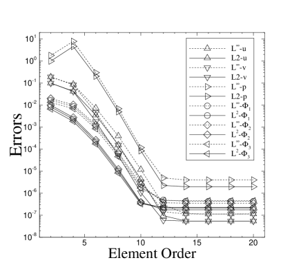
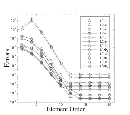
In the first group of tests we fix the time step size at $\Delta t=0.001$ and final integration time at $t_{f}=0.1$, and vary the element order systematically between $2$ and $20$. Figure 1(a) shows the errors of the numerical solution in $L^{\infty}$ and $L^{2}$ norms for the velocity, pressure and the phase-field variables ($\phi_{1}$, $\phi_{2}$, $\phi_{3}$) at $t=t_{f}$ as a function of the element order, obtained with the volume fractions as the order parameters (see equation (26)). It is evident that the numerical errors decrease exponentially as the element order increases and is below about $12$. As the element order increases beyond $12$, the error curves level off owing to the saturation with the temporal truncation errors. Figure 1(c) shows the corresponding error results obtained using the re-scaled density differences as the order parameters (see (33)). One can similarly observe an exponential spatial convergence rate.

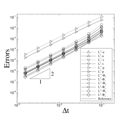
In the second group of convergence tests we fix the element order at a large value $18$ and the final integration time at $t_{f}=1.0$. Then we vary the time step size systematically between $\Delta t=0.0015625$ and $\Delta t=0.1$. In Figure 1(b) we plot the $L^{\infty}$ and $L^{2}$ errors of the numerical solution at $t=t_{f}$ against the analytic solution for different variables as a function of $\Delta t$, obtained with the volume fractions as the order parameters. The error curves exhibit a second-order temporal convergence rate. Figure 1(d) contains the corresponding results obtained with the re-scaled density differences as the order parameters, showing similarly a second-order temporal convergence rate.

4.2 Floating Oil Lens on Water Surface

Figure 2: Initial configuration for the three-phase problem of floating oil lens on water surface.

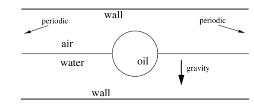
In this section we look into an air-water-oil three-phase problem, where the oil forms a liquid lens floating on the water surface at equilibrium. We quantitatively compare the simulation results with the theory by Langmuir and de Gennes Langmuir1933 ; deGennesBQ2003 to show that our method produces physically accurate results. A similar liquid-lens problem was considered in Dong2014 using the special set of order parameters defined by (24). Here we simulate the problem with general order parameters, and investigate the effects of several sets of physical parameters on the air-water-oil configurations.

Consider the flow domain depicted in Figure 2, $-\frac{L}{2}\leqslant x\leqslant\frac{L}{2}$ and $0\leqslant y\leqslant\frac{4}{5}L$, where $L=4cm$. The top and the bottom of the domain ($y=0$ and $\frac{4}{5}L$) are two solid walls. In the horizontal direction the domain is periodic at $x=\frac{L}{2}$ and $x=-\frac{L}{2}$. At $t=0$, the domain is filled with air in its top half and filled with water in its bottom half, and a circular oil drop of radius $R_{0}=\frac{L}{5}$ is held at rest on the water surface with its center located at $\mathbf{x}_{c}=(x_{c},y_{c})=(0,\frac{2}{5}L)$. It is assumed that the gravity is in the $-y$ direction, and that there is no initial flow. The system is then released, and evolves to equilibrium due to the interactions among the three fluid components and the effects of the gravity and the surface tensions. Our goal is investigate the effects of several physical parameters on the equilibrium configurations of the oil.

density [$kg/m^{3}$]:	air	$1.2041$	water	$998.207$	oil	$577$ (or varied)
dynamic viscosity [$kg/(m\cdot s)$]:	air	$1.78E-5$	water	$1.002E-3$	oil	$9.15E-2$
surface tension [$kg/s^{2}$]:	air/water	$0.0728$	oil/water	$0.04$	air/oil	$0.065$ (or varied)
gravity [$m/s^{2}$]:	$9.8$

Table 3: Physical parameter values for the air-water-oil three phase problem.

Table 3 lists the values of the physical parameters, including the densities, dynamic viscosities, and the pairwise surface tensions of the three fluids involved in this problem. We use $L$ as the characteristic length scale, and choose a characteristic velocity scale $U_{0}=\sqrt{g_{r0}L}$, where $g_{r0}=1m/s^{2}$. We assign the air, water and oil as the first, second and third fluid, respectively. All the flow variables and physical parameters are then non-dimensionalized based on the normalization constants specified in Table 1. We set $g_{i}=0$ ($1\leqslant i\leqslant N-1$) in (13c) for the simulations.

In order to simulate the problem, we discretize the domain using $160$ equal-sized quadrilateral elements, with $20$ elements along the $x$ direction and $8$ along the $y$ direction. The element order is $16$ in the simulations. The algorithm developed in Section 3 has been used to solve the coupled system of governing equations. For the boundary conditions, at the top/bottom walls, we impose the condition (60) with $\mathbf{w}=0$ for the velocity and the conditions (61a) and (61b) for the phase field functions. In the horizontal direction, all the flow variables (velocity, pressure, phase field functions) are set to be periodic. Table 4 summarizes the numerical parameter values in the simulations.

parameters	values
$\lambda_{ij}$	computed based on (58)
$\eta/L$	$0.0075$
$\beta$	computed based on (62)
$m_{i}\tilde{\rho}_{1}U_{0}/L$, $1\leqslant i\leqslant N-1$	$10^{-7}/\lambda_{max}$, where $\lambda_{max}=\frac{\max\{\lambda_{ij}\}}{\tilde{\rho}_{1}U_{0}^{2}L^{2}}$
$\hat{s}_{i}$	$2\eta^{2}\sqrt{\hat{\lambda}_{i}}$
$\rho_{0}$	$\min\left\{\tilde{\rho}_{i}\right\}_{1\leqslant i\leqslant N}$
$\nu_{0}$	$2\max\left\{\frac{\tilde{\mu}_{i}}{\tilde{\rho}_{i}}\right\}_{1\leqslant i\leqslant N}$
$U_{0}\Delta t/L$	$2.5\times 10^{-6}$
$J$ (temporal order)	$2$

Table 4: Simulation parameter values for the air-water-oil three phase problem.

We employ the formulation with the volume fractions as the order parameters, defined in (26), for simulations of all the cases in this section. We have also simulated several selected cases using the formulation with the re-scaled volume fraction differences as the order parameters, as defined in (29). The initial velocity is set to zero. The initial phase field functions are set to

$$\phi_{i}(\mathbf{x},t=0)=c_{i0},\quad 1\leqslant i\leqslant N-1,$$ (99)

for the order parameters defined by (26), and

$$\phi_{i}(\mathbf{x},t=0)=\frac{1}{2}+\frac{1}{2}\left(c_{i0}-c_{N0}\right),\quad 1\leqslant i\leqslant N-1,$$ (100)

for the order parameters defined by (29). In these equations, $c_{i0}$ ($1\leqslant i\leqslant N$) are the initial volume fractions given by ($N=3$)

$$c_{10}=\left[1-\Theta(x,x_{c}-R_{0})+\Theta(x,x_{c}+R_{0})\right]\frac{1}{2}\left(1+\tanh\frac{y-y_{c}}{\sqrt{2}\eta}\right)\\ +\left[\Theta(x,x_{c}-R_{0})-\Theta(x,x_{c}+R_{0})\right]\frac{1}{2}\left(1+\tanh\frac{\left|\mathbf{x}-\mathbf{x}_{c}\right|-R_{0}}{\sqrt{2}\eta}\right)\Theta(y,y_{c}),$$

$$c_{20}=\left[1-\Theta(x,x_{c}-R_{0})+\Theta(x,x_{c}+R_{0})\right]\frac{1}{2}\left(1-\tanh\frac{y-y_{c}}{\sqrt{2}\eta}\right)\\ +\left[\Theta(x,x_{c}-R_{0})-\Theta(x,x_{c}+R_{0})\right]\frac{1}{2}\left(1+\tanh\frac{\left|\mathbf{x}-\mathbf{x}_{c}\right|-R_{0}}{\sqrt{2}\eta}\right)\left[1-\Theta(y,y_{c})\right],$$

$$c_{30}=\frac{1}{2}\left(1-\tanh\frac{\left|\mathbf{x}-\mathbf{x}_{c}\right|-R_{0}}{\sqrt{2}\eta}\right),$$

where $\Theta(x,a)$ is the unit step function, assuming unit value if $x\geqslant a$ and zero otherwise.

(a) (b) (c)

Figure 3: Effect of oil density on equilibrium oil puddle configurations (3 fluid phases): (a) $\rho_{o}=300kg/m^{3}$, (b) $\rho_{o}=500kg/m^{3}$, (c) $\rho_{o}=750kg/m^{3}$. Results obtained using volume fractions $c_{i}$ ($1\leqslant i\leqslant N-1$) as order parameters.

The physics of floating liquid lenses for three phases was discussed in Langmuir Langmuir1933 and de Gennes et al deGennesBQ2003 (pages 54–56). The equilibrium oil-drop shape is determined by the interplay of the gravity and the three pair-wise surface tensions, and also influenced by the three densities. When the gravity effect dominates, the oil will form a puddle on the water surface. If the surface tension effects dominate, the oil-drop shape will consist of two circular caps in two dimensions or two spherical caps in three dimensions. One can approximately determine which effect is dominant by comparing the characteristic drop size with the three capillary lengths associated with the three types of interfaces; see deGennesBQ2003 .

We will investigate the effects on the equilibrium oil configurations of two physical parameters: the oil density and the air-oil surface tension.

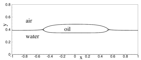
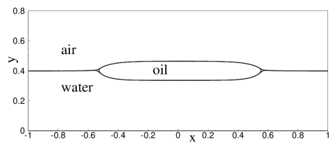
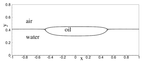
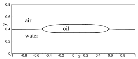
Let us first consider the effect of the oil density. In this group of tests, we vary the density of the oil systematically ranging from $300kg/m^{3}$ to $750kg/m^{3}$, and fix all the other physical parameters at values given in Table 3 (air-oil surface tension fixed at $0.065kg/s^{2}$). In Figure 3 we show the equilibrium oil configurations corresponding to three oil-density values $\rho_{o}=300kg/m^{3}$, $500kg/m^{3}$ and $750kg/m^{3}$. They are obtained using the volume fractions as the order parameters. Plotted are the contours of volume fractions $c_{i}=\frac{1}{2}$ ($i=1,2,3$) for the three fluids. One can note the “star”-shaped regions around the three-phase contact lines in these figures. This is because in these regions none of the three fluids has a volume fraction larger than $\frac{1}{2}$. It is evident that the oil forms puddles floating on the water surface. Subtle differences can be noticed in their shapes, for example, in the curvature of the oil profiles not far from the three-phase contact lines. In addition, the immersion depths of the oil in the water are notably different as the oil density changes.

(a) (b)

Figure 4: Equilibrium oil-puddle configurations for oil density $\rho_{o}=400kg/m^{3}$ obtained using (a) volume fractions $c_{i}$ ($1\leqslant i\leqslant N-1$) as order parameters, and (b) re-scaled volume fraction differences as order parameters (equation (29)).

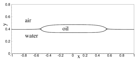
The simulation results obtained using different sets of order parameters are similar, as is expected. This is shown by Figure 4. Here we compare the equilibrium oil configurations, as shown by the contour levels $c_{i}=\frac{1}{2}$, corresponding to the oil density $\rho_{0}=400kg/m^{3}$ obtained using the volume fractions as the order parameters (equation (26)), see Figure 4(a), and using the re-scaled volume fraction differences as the order parameters (equation (29)), see Figure 4(b). The results are qualitatively similar.

Figure 5: Comparison of the oil-puddle thickness as a function of the oil density between current simulations and the Langmuir-de Gennes theory deGennesBQ2003 for three fluid phases.

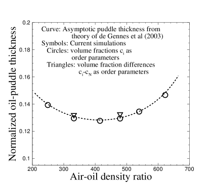
We have computed the thickness of the oil puddles at equilibrium, defined as the distance along the vertical direction between the upper and lower puddle surfaces, corresponding to different oil densities. The symbols in Figure 5 show the normalized oil-puddle thickness as a function of the normalized oil density obtained from the current simulations. The results from both sets of order parameters have been included in this figure, differentiated using different symbols. It is shown in Langmuir1933 ; deGennesBQ2003 that for three fluid phases, when the gravity is dominant (i.e. oil forming puddles), the puddle thickness can be explicitly expressed in terms of the known physical parameters as follows,

$$e_{c}=\sqrt{\frac{2\left(\sigma_{ao}+\sigma_{ow}-\sigma_{ow}\right)\rho_{w}}{(\rho_{w}-\rho_{o})\rho_{o}g_{r}}},$$ (101)

where $e_{c}$ is the asymptotic puddle thickness when the gravity is dominant, $g_{r}$ is the gravitational acceleration, $\rho_{w}$ and $\rho_{o}$ are respectively the water and oil densities, and $\sigma_{ao}$, $\sigma_{aw}$ and $\sigma_{ow}$ are respectively the air-oil, air-water, and oil-water surface tensions. For comparison, the dashed curve in Figure 5 shows the relation between $e_{c}$ and $\rho_{o}$ given by (101). The results from the current simulations agree with the results based on the theory of Langmuir1933 ; deGennesBQ2003 quite well.

(a) (b)

Figure 6: Equilibrium configurations of an oil puddle on the air-water interface corresponding to air-oil surface tensions: (a) $0.065kg/s^{2}$, (b) $0.085kg/s^{2}$. All other physical parameters are fixed. Results are obtained with the volume fractions $c_{i}$ ($1\leqslant i\leqslant N-1$) as the order parameters.

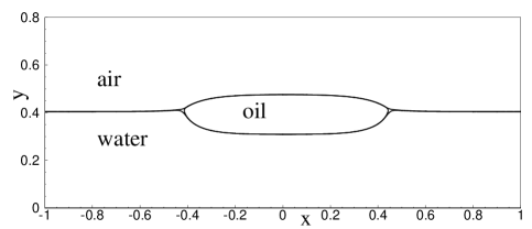
We next look into the effect of the air-oil surface tension on the equilibrium configuration of this three-phase system. In this group of tests we vary the air-oil surface tension systematically between $0.055kg/s^{2}$ and $0.095kg/s^{2}$, while fixing all the other parameters at those values in Table 3 (oil density is $577kg/m^{3}$). Figure 6 shows the equilibrium configurations of the system (contour lines $c_{i}=\frac{1}{2}$, $1\leqslant i\leqslant 3$) corresponding to the air-oil surface tensions $0.065kg/s^{2}$ and $0.085kg/s^{2}$. They are obtained with the volume fractions as the order parameters. The oil forms a puddle, and the puddle size and thickness have a clear dependence on the value of the air-oil surface tension. A larger air-oil surface tension leads to a smaller but thicker oil puddle at equilibrium.

Figure 7: Comparison between current simulations and the Langmuir-de Gennes theory deGennesBQ2003 for air-water-oil three fluid phases: Oil-puddle thickness squared as a function of the air-oil surface tension. Circles denote results obtained with the volume fractions as order parameters. Triangles denote results obtained with the re-scaled volume-fraction differences as order parameters.

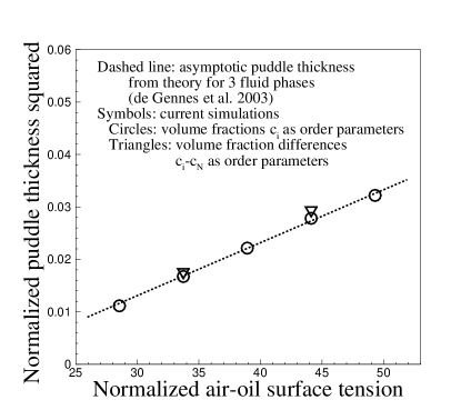
The quantitative relationship between the oil-puddle thickness and the air-oil surface tension is demonstrated by Figure 7. Here we plot the puddle-thickness squared as a function of the air-oil surface tension. The symbols represent results from the simulations. The circles denote the results obtained using the volume fractions as the order parameters (equation (26)), and the triangles denote those obtained using the re-scaled volume-fraction differences (equation (29)) as the order parameters. For comparison, the theoretical relationship between these two quantities, see equation (101), due to Langmuir1933 ; deGennesBQ2003 is also shown in this figure, by the dashed line. It can be observed that the data from current simulations are in good agreement with the theory.

To summarize, the floating liquid lens problem studied in this section involves multiple fluid phases, multiple pairwise surface tensions, gravity, large density ratios and viscosity ratios. The quantitative comparisons between current simulations and the theory of Langmuir and de Gennes Langmuir1933 ; deGennesBQ2003 show that, the physical formulations and the numerical algorithm with general order parameters developed in the current work produce physically accurate results. The results of this section also demonstrate the significant effects of the densities and the pairwise surface tensions on the configurations of this three-phase system.

4.3 Dynamics of a Four-Phase Fluid Mixture

In this section we look into the dynamics of a mixture of four immiscible incompressible fluids. The goal is to demonstrate the capability of our method from Section 3 for simulating dynamical problems.

(a) (b) (c) (d)

(e) (f) (g) (h)

(i) (j) (k) (l)

(m) (n) (o) (p)

Figure 8: Volume fraction contours ($c_{i}=\frac{1}{2}$) showing fluid drops impacting water surface (4 fluid phases): (a) $t=0.076$, (b) $t=0.176$, (c) $t=0.26$, (d) $t=0.332$, (e) $t=0.46$, (f) $t=0.608$, (g) $t=0.712$, (h) $t=0.796$, (i) $t=0.836$, (j) $t=0.888$, (k) $t=0.944$, (l) $t=1.128$, (m) $t=1.196$, (n) $t=1.504$, (o) $t=2.208$, (p) $t=3.384$.

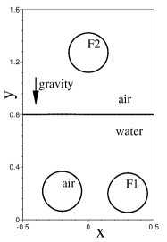
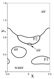
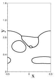
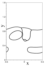
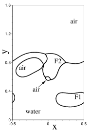
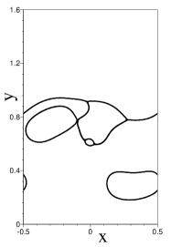
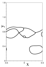
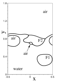
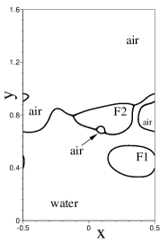
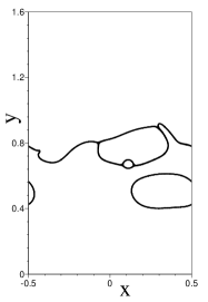
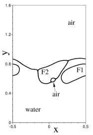
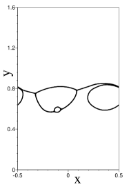
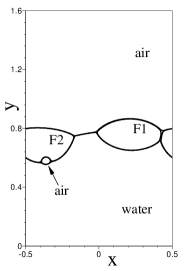
The setting of this problem is as follows. Consider the rectangular flow domain as shown in Figure 8(a), $-\frac{L}{2}\leqslant x\leqslant\frac{L}{2}$ and $0\leqslant y\leqslant\frac{8}{5}L$, where $L=2cm$. The top and bottom sides of the domain are solid walls. If any of the fluid interfaces involved in this problem intersects with the walls, the contact angle is assumed to be $90^{0}$. In the horizontal direction the domain is assumed to be periodic at $x=\pm\frac{L}{2}$. The gravity is assumed be along the $-y$ direction. At $t=0$, the top half of the domain is filled with air, and the bottom half is filled with water. A circular drop (diameter $0.3L$) of a fluid, denoted by “F2”, is suspended in the air at rest. Simultaneously, an air bubble and a drop of another fluid, denoted by “F1”, both circular initially with diameter $0.3L$, are trapped in the water. The centers of the air bubble and the fluid drops have the following coordinates

$$\left\{\begin{split}&\mathbf{x}_{F1}=\left(x_{F1},y_{F1}\right)=(0.3L,0.2L),\quad\text{(F1 drop)}\\ &\mathbf{x}_{F2}=\left(x_{F2},y_{F2}\right)=(0,1.3L),\quad\text{(F2 drop)}\\ &\mathbf{x}_{a}=\left(x_{a},y_{a}\right)=(-0.2L,0.2L),\quad\text{(air bubble)}.\end{split}\right.$$ (102)

The four types of fluids (air, water, F1, and F2) are assumed to be incompressible and all immiscible with one another, and it is assumed that there is no initial velocity. The system is then released. The liquid drops and the air bubble fall through the air or rise through the water, and then impact the water surface. The objective is to simulate the dynamics of this process.

density[kg/m3]	air	$1.2041$	water	$998.207$	F1	$400$	F2	$870$
dynamic viscosity[kg/(m$\cdot$s)]	air	$1.78E-5$	water	$1.002E-3$	F1	$0.02$	F2	$0.0915$
surface tension[kg/s2]	air/water	$0.0728$	air/F1	$0.06$	air/F2	$0.055$
	water/F1	$0.045$	water/F2	$0.044$	F1/F2	$0.048$
gravity [m/s2]	9.8

Table 5: Physical parameter values for the air-water-F1-F2 four phase problem.

In Table 5 we list the values of the physical parameters involved in this problem, including the densities and dynamic viscosities of the four fluids, and the six pairwise surface tensions among them. We assign the air, water, F2 and F1 fluids respectively as the first, second, third and fourth fluid. We choose $L$ as the characteristic length scale and $U_{0}=\sqrt{g_{r0}L}$ as the characteristic velocity scale, where $g_{r0}=1m/s^{2}$. The non-dimensionalization of the problem then follows in a straightforward fashion based on the constants given in Table 1. We set $g_{i}=0$ ($1\leqslant i\leqslant N-1$) in (13c) in the simulations.

In order to simulate the problem, we discretize the domain using $1440$ quadrilateral elements of equal sizes, with $30$ elements in the $x$ direction and $48$ elements in the $y$ direction. An element order of $12$ (with over-integration) has been used in the simulations for all elements. The algorithm developed in Section 3, and the formulation with the volume fractions $c_{i}$ ($1\leqslant i\leqslant N-1$, where $N=4$) as the order parameters as defined by (26), have been employed to integrate this four-phase system in time. For the boundary conditions on the top and bottom walls, the condition (60) with $\mathbf{w}=0$ has been imposed for the velocity, and the conditions (61a) and (61b) have been imposed for the phase field functions $\phi_{i}$ ($1\leqslant i\leqslant 3$). In the horizontal direction, periodic conditions have been imposed at $x=\pm\frac{L}{2}$ for all flow variables. The initial velocity is set to zero. The initial phase field functions are set according to equation (99) with $N=4$, where the initial volume fractions are

$$\begin{split}c_{10}=&\frac{1}{2}\left(1+\tanh\frac{y-y_{w}}{\sqrt{2}\eta}\right)\left[1-\frac{1}{2}\left(1-\tanh\frac{\left|\mathbf{x}-\mathbf{x}_{F2}\right|-R_{0}}{\sqrt{2}\eta}\right)\right]+\frac{1}{2}\left(1-\tanh\frac{\left|\mathbf{x}-\mathbf{x}_{a}\right|-R_{0}}{\sqrt{2}\eta}\right),\end{split}$$

$$c_{20}=\frac{1}{2}\left(1-\tanh\frac{y-y_{w}}{\sqrt{2}\eta}\right)\left[1-\frac{1}{2}\left(1-\tanh\frac{\left|\mathbf{x}-\mathbf{x}_{a}\right|-R_{0}}{\sqrt{2}\eta}\right)-\frac{1}{2}\left(1-\tanh\frac{\left|\mathbf{x}-\mathbf{x}_{F1}\right|-R_{0}}{\sqrt{2}\eta}\right)\right],$$

$$c_{30}=\frac{1}{2}\left(1-\tanh\frac{\left|\mathbf{x}-\mathbf{x}_{F2}\right|-R_{0}}{\sqrt{2}\eta}\right),$$

$$c_{40}=\frac{1}{2}\left(1-\tanh\frac{\left|\mathbf{x}-\mathbf{x}_{F1}\right|-R_{0}}{\sqrt{2}\eta}\right),$$

where $y_{w}=\frac{4}{5}L$ is the initial position of the water surface in the $y$ direction, and $R_{0}=0.15L$ is the initial radii of the air bubble and fluid drops.

parameters	values
$\lambda_{ij}$	computed based on (58)
$\eta/L$	$0.005$
$\beta$	computed based on (62)
$m_{i}\tilde{\rho}_{1}U_{0}/L$, $1\leqslant i\leqslant N-1$	$2\times 10^{-8}/\lambda_{max}$, where $\lambda_{max}=\frac{\max\{\lambda_{ij}\}}{\tilde{\rho}_{1}U_{0}^{2}L^{2}}$
$\hat{s}_{i}$	$2\eta^{2}\sqrt{\hat{\lambda}_{i}}$
$\rho_{0}$	$\min\left\{\tilde{\rho}_{i}\right\}_{1\leqslant i\leqslant N}$
$\nu_{0}$	$5\max\left\{\frac{\tilde{\mu}_{i}}{\tilde{\rho}_{i}}\right\}_{1\leqslant i\leqslant N}$
$U_{0}\Delta t/L$	$2\times 10^{-6}$
$J$ (temporal order)	$2$

Table 6: Simulation parameter values for the air-water-F1-F2 four phase problem. $N=4$ in this table.

Table 6 summarizes the values of all the numerical parameters involved in the algorithm and the simulations.

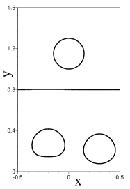
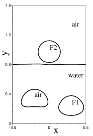
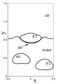
We now look into the dynamics of this four-phase flow. In Figure 8 we show a temporal sequence of snapshots of the fluid interfaces in the flow by plotting the contour lines of the volume fractions $c_{i}=\frac{1}{2}$ ($1\leqslant i\leqslant 4$). From Figures 8(a)–(c), one can observe that upon release the F2 drop falls rapidly through the air due to the gravity, and is about to impact the water surface (Figure 8c). Its profile maintains essentially the original shape during the falling process. Simultaneously, the air bubble and the F1 drop rise through the water due to buoyancy, albeit much more slowly compared to the falling F2 drop. They experience significant deformations in their shapes. The air bubble has the shape of a “cap”, with a flat underside (Figure 8c). Figure 8(d) shows that the F2 drop impacts the water surface, and generates a ripple that spreads outward. The F2 drop traps a pocket of air at its underside. Later on, the F2 fluid forms a pool floating on the water surface and the trapped air pocket forms a small bubble (Figure 8(e)). Figures 8(f) through 8(k) show the interaction between the rising air bubble and the floating F2 pool on the water surface. Notice that the F2 fluid is mostly immersed in the water owing to the small density contrast between F2 and water (see e.g. Figure 8(g)). As the air bubble rises, it approaches and “kisses” the F2 fluid immersed in the water (Figures 8(g)–(j)), and then pulls apart (Figure 8(k)). This interaction and the motion of the air bubble has caused a dramatic deformation in the profile of the F2 fluid (Figures 8(i)–(k)). One also observes that, during this period of time, the upward motion of the F1 drop appears to have stalled (Figures 8(f)–(j)), but the drop exhibits significant deformations in shape. Figures 8(k)–(m) show that the air bubble touches the water surface and merges with the bulk of air above the water. As time goes on, the F1 drop rises slowly through the water and forms a floating F1 drop on the water surface (Figures 8(n)–(p)). Eventually, the water surface becomes mostly covered by the floating F1 and F2 drops, and the F2 drop has a small air bubble trapped at its underside (Figure 8(p)).

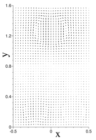(a) (b) (c) (d)

(e) (f) (g) (h)

(i) (j) (k) (l)

(m) (n) (o) (p)

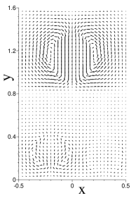
Figure 9: Velocity fields of fluid drops impacting water surface (4 fluid phases): (a) $t=0.076$, (b) $t=0.176$, (c) $t=0.26$, (d) $t=0.332$, (e) $t=0.46$, (f) $t=0.608$, (g) $t=0.712$, (h) $t=0.796$, (i) $t=0.836$, (j) $t=0.888$, (k) $t=0.944$, (l) $t=1.128$, (m) $t=1.196$, (n) $t=1.504$, (o) $t=2.208$, (p) $t=3.384$. Velocity vectors are plotted on every 15-th quadrature points in each direction on each element.

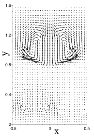
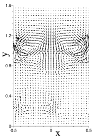
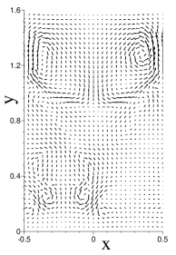
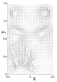
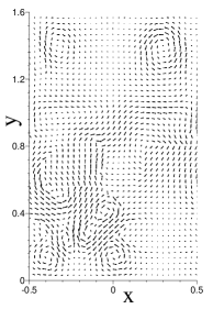
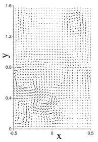
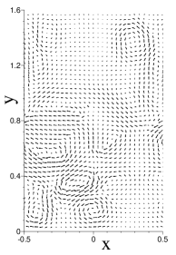
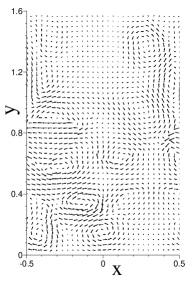
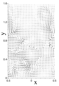
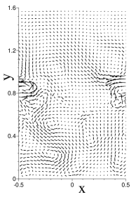
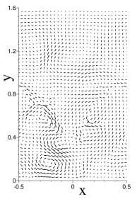
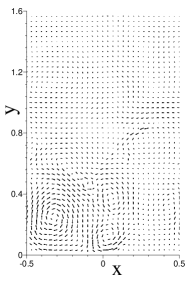
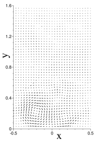
We further illustrate the dynamical features of this flow by looking into the velocity distributions. Figure 9 is a temporal sequence of snapshots of the velocity fields of this four-phase flow at the same time instants as those in Figure 8. In order to make the figures clearer, the velocity vectors have been plotted on every $15$-th quadrature point in each direction within each element. Figures 9(a)–(c) indicate that the falling F2 drop induces a velocity field inside the air, forming a pair of vortices near the shoulders of the F2 drop (see e.g. Figures 9(b)–(c)). On the other hand, the velocity inside the F2 drop is largely uniform. Prior to the impact on the water surface (Figure 9c), the air is squeezed out from between the F2 drop and the water surface, resulting in a strong lateral air flow just above the water surface. Upon impact, the strong air flow produces a pair of vortices behind (i.e. above) either side of the F2 drop (Figure 9d), noting the periodicity in the horizontal direction. The pair of vortices subsequently travel upward in the air and dies down gradually over time (Figures 9(e)–(k)). Simultaneously, the rise of the air bubble through the water induces a pair of vortices behind (see e.g. Figure 9d). A pair of vortices can also be recognized behind the F1 drop; see e.g. Figure 9(f). An interaction of these two pairs of vortices in the water can be observed (Figures 9(f)–(k)). Subsequently, the merger of the air bubble and the bulk of air generates an energetic air flow near the water surface (Figures 9(l)–(m)). Figures 9(n)–(p) show that the velocity field inside the water, and also in the air, dies down as the F1 drop rises to the water surface and the system approaches an equilibrium state.

5 Concluding Remarks

The contributions of the current work can be summarized in terms of the following three aspects:

• We have presented a set of N-phase physical formulations for a class of general order parameters. They generalize the N-phase formulation presented in Dong2014 , which is based on a special set of order parameters. This generalization has three implications: (1) The set of ($N-1$) phase field equations becomes more strongly coupled with one another, in particular, the inertia terms $\frac{\partial\phi_{i}}{\partial t}$ are all coupled with one another; (2) It makes it possible to come up with an explicit form for the mixing energy density coefficients $\lambda_{ij}$; (3) Numerical solution of the coupled phase field equations becomes more challenging.

• We have provided an explicit form for computing the mixing energy density coefficients $\lambda_{ij}$ with general order parameters. Note that the method in Dong2014 requires the solution of a linear algebraic system to determine $\lambda_{ij}$. In contrast, $\lambda_{ij}$ in the current paper are given in an explicit form, which applies to general order parameters, including the special order-parameter set employed in Dong2014 .

• We have developed an efficient algorithm for numerically solving the phase field equations with general order parameters. The algorithm transforms the ($N-1$) strongly-coupled 4-th order phase field equations for general order parameters into $2(N-1)$ Helmholtz type equations that are completely de-coupled from one another. The computational complexity of the current algorithm for general order parameters is comparable to that of Dong2014 for the special set of order parameters. The advantage with the special set of order parameters of Dong2014 lies in that the phase field equations have a simpler form. The current work shows that, even though the phase field equations have a more complicated form with general order parameters, the computational work involved in the numerical solutions of these equations is essentially the same as that for the simpler phase field equations with the special set of order parameters of Dong2014 .

We have presented several example problems to demonstrate the accuracy and capability of the physical formulations and the numerical algorithm developed herein. These test problems involve multiple fluid phases, large density contrasts, large viscosity contrasts, and multiple pairwise surface tensions. Several different sets of order parameters have been employed in the simulations. By comparing with the theory of Langmuir and de Gennes Langmuir1933 ; deGennesBQ2003 , we have shown that the formulations and the numerical algorithm developed herein have produced physically accurate results for multiple fluid phases. The simulation results also demonstrate the complex dynamics induced by the interactions among multiple types of fluid interfaces.

It is instructive to compare the general order parameters discussed here for N-phase flows with the order parameter for two-phase flows. There exists only one independent order parameter for a two-phase system, and different order parameters have been used by different researchers in the literature. Several choices of the order parameter for two phases are touched on in e.g. AbelsGG2012 , and the resultant two-phase phase field equation would usually only require a simple re-scaling for a different choice of the order parameter.

On the other hand, for an N-phase system there are ($N-1$) independent order parameters. The possibilities for choosing the ($N-1$) order parameters are much broader, and different choices lead to varying degrees of complexity in the resulting phase field equations. The class of order parameters considered in the current work, equation (12), has a linear relation between ($\rho_{i}-\rho_{N}$) and $\phi_{j}$. One can readily imagine even broader classes of order parameters, e.g.

$$\varphi_{i}(\vec{\phi})=\rho_{i}(\vec{\phi})-\rho_{N}(\vec{\phi})=f_{i}(\vec{\phi}),\quad 1\leqslant i\leqslant N-1,$$ (103)

where $f_{i}(\vec{\phi})$ are ($N-1$) given functions and in general can be nonlinear. This, however, will lead to even more complicated forms for the phase field equations. Note that, regardless of the set of order parameters being employed, the phase field equations all represent the mass balance relations for the $N$ individual fluid phases. We hold the view that the formulations with different order parameters are merely different representations of the N-phase system, and that the different representations should be equivalent to one another. This is an embodiment of the representation invariance principle MaW2014 . The explicit expressions for the mixing energy density coefficients $\lambda_{ij}$ derived in the current work are a direct result of this principle.

Appendix A: Unique Solvability of $\lambda_{ij}$ Linear Algebraic System

In this Appendix we prove that the linear algebraic system about $\lambda_{ij}$ derived in Dong2014 for the special set of order parameters defined by (24) has a unique solution for any $N\geqslant 2$. The unique solvability of that system for $N\geqslant 4$ is an un-settled issue in Dong2014 .

The idea of the proof is as follows. We will show that the system of equations about $\Lambda_{ij}$ ((46) and (48)) in the current work, under a non-singular transform, is equivalent to the linear algebraic system about $\lambda_{ij}$ in Dong2014 for the special set of order parameters defined by (24). Since the system consisting of (46) and (48) has a unique solution for any $N\geqslant 2$, the linear system from Dong2014 must also have a unique solution.

The following is the linear algebraic system about $\lambda_{ij}$ from Dong2014 , which is based on the set of order parameters defined by (24),

$$\sum_{i,j=1}^{N-1}L_{i}^{kl}L_{j}^{kl}\lambda_{ij}=\frac{9}{2}\frac{\eta^{2}}{\beta^{2}}\sigma_{kl}^{2},\qquad 1\leqslant k<l\leqslant N,$$ (104)

where

$$L_{i}^{kl}=\left\{\begin{array}[]{ll}\frac{\tilde{\rho}_{k}}{\tilde{\rho}_{k}+\tilde{\rho}_{N}}\delta_{ik}-\frac{\tilde{\rho}_{l}}{\tilde{\rho}_{l}+\tilde{\rho}_{N}}\delta_{il},&1\leqslant k<l\leqslant N-1,\ 1\leqslant i\leqslant N-1,\\ \frac{\tilde{\rho}_{i}}{\tilde{\rho}_{i}+\tilde{\rho}_{N}}\delta_{ik}+\frac{\tilde{\rho}_{N}}{\tilde{\rho}_{i}+\tilde{\rho}_{N}},&1\leqslant k<l=N,\ 1\leqslant i\leqslant N-1.\end{array}\right.$$ (105)

This is a system of $\frac{1}{2}N(N-1)$ equations about $\frac{1}{2}N(N-1)$ unknowns, noting the symmetry $\lambda_{ij}=\lambda_{ji}$ ($1\leqslant i,j\leqslant N-1$).

We next show that the linear system consisting of (46) and (48) about $\Lambda_{ij}$ can be transformed to the system (104) about $\lambda_{ij}$, under the transform (59) between $\mathbf{A}$ and $\bm{\Lambda}$. Re-write (59) as

$$\begin{bmatrix}\Lambda_{ij}\end{bmatrix}_{(N-1)\times(N-1)}=\bm{\Lambda}=\mathbf{Z}^{-1}\mathbf{L}^{-1}\mathbf{A}\mathbf{L}^{-1}\mathbf{Z}^{-1}=\bm{\Lambda}_{1}\mathbf{L}^{-1}\mathbf{A}\mathbf{L}^{-1}\bm{\Lambda}_{1}=4\mathbf{R}^{T}\mathbf{AR}$$ (106)

where we have used equation (55) and $\bm{\Lambda}_{1}$ is defined in (38), and

$$\mathbf{R}=\frac{1}{2}\mathbf{L}^{-1}\bm{\Lambda}_{1}=\begin{bmatrix}r_{ij}\end{bmatrix}_{(N-1)\times(N-1)},\qquad r_{ij}=\frac{\tilde{\rho}_{i}}{\tilde{\rho}_{i}+\tilde{\rho}_{N}}\delta_{ij}+\frac{\tilde{\rho}_{N}}{\tilde{\rho}_{i}+\tilde{\rho}_{N}}=L_{i}^{jN}.$$ (107)

First consider the case $1\leqslant k<l\leqslant N-1$. Equation (48) becomes

$$\begin{split}\frac{9}{2}\frac{\eta^{2}}{\beta^{2}}\sigma_{kl}^{2}&=\frac{1}{4}\left(\Lambda_{kk}+\Lambda_{ll}-2\Lambda_{kl}\right)\\ &=\left(\frac{\tilde{\rho}_{k}}{\tilde{\rho}_{k}+\tilde{\rho}_{N}}\right)^{2}\lambda_{kk}+\left(\frac{\tilde{\rho}_{l}}{\tilde{\rho}_{l}+\tilde{\rho}_{N}}\right)^{2}\lambda_{ll}-2\frac{\tilde{\rho}_{k}}{\tilde{\rho}_{k}+\tilde{\rho}_{N}}\frac{\tilde{\rho}_{l}}{\tilde{\rho}_{l}+\tilde{\rho}_{N}}\lambda_{kl}\\ &=\left(L_{k}^{kl}\right)^{2}\lambda_{kk}+\left(L_{l}^{kl}\right)^{2}\lambda_{ll}+2L_{k}^{kl}L_{l}^{kl}\lambda_{kl}\\ &=\sum_{i,j=1}^{N-1}L_{i}^{kl}L_{j}^{kl}\lambda_{ij},\qquad 1\leqslant k<l\leqslant N-1\end{split}$$ (108)

where we have used (106) and (105). Therefore Equation (48) is transformed to (104) for the case $1\leqslant k<l\leqslant N-1$. Next consider the case $1\leqslant k<l=N$. Equation (46) becomes

$$\begin{split}\frac{9}{2}\frac{\eta^{2}}{\beta^{2}}\sigma_{kN}^{2}&=\frac{1}{4}\Lambda_{kk}=\sum_{i,j=1}^{N-1}r_{ik}r_{jk}\lambda_{ij}=\sum_{i,j=1}^{N-1}L_{i}^{kN}L_{j}^{kN}\lambda_{ij},\qquad 1\leqslant k<l=N\end{split}$$ (109)

where we have used (106), (105), and (107). Therefore, equation (46) is transformed to (104) for the case $1\leqslant k<l=N$.

Since the transform (59) (or equivalently (106)) is non-singular, we conclude that the linear system consisting of (46) and (48) is equivalent to the linear system given by (104). We can then conclude that the linear system (104) about $\lambda_{ij}$ has a unique solution for any $N\geqslant 2$, and that its solution is given by (59), in which $\bm{\Lambda}$ is given by (37), (46) and (49).

Appendix B: Algorithm for N-Phase Momentum Equations

In this Appendix we present an algorithm for the N-phase momentum equations, (13a) and (13b), together with the velocity boundary condition, (60). While it is also based on a velocity correction-type strategy to de-couple the pressure and velocity computations, this scheme is different in formulation than that of Dong2014 , and it results in a smaller pressure error than the latter. The algorithmic formulation here for the N-phase momentum equations, however, can be traced to that we developed in DongS2012 for two-phase flows.

We assume that the phase field variables $\phi_{i}$ ($1\leqslant i\leqslant N-1$) are known, and our goal is to compute the velocity and pressure from (13a) and (13b). Let

$$P=p+\sum_{i,j=1}^{N-1}\frac{\lambda_{ij}}{2}\nabla\phi_{i}\cdot\nabla\phi_{j}$$ (110)

denote an auxiliary pressure, which will also be loosely referred to as pressure hereafter. We can then transform (13a) into

$$\frac{\partial\mathbf{u}}{\partial t}+\mathbf{u}\cdot\nabla\mathbf{u}=\frac{1}{\rho}\nabla P+\frac{\mu}{\rho}\nabla^{2}\mathbf{u}+\frac{1}{\rho}\nabla\mu\cdot\mathbf{D}(\mathbf{u})-\frac{1}{\rho}\sum_{i,j=1}^{N-1}\lambda_{ij}\nabla^{2}\phi_{j}\nabla\phi_{i}+\frac{1}{\rho}\mathbf{f}.$$ (111)

Given ($\mathbf{u}^{n}$, $P^{n}$, $\phi_{i}^{n+1}$), our algorithm for (111) and (13b) successively computes $P^{n+1}$ and $\mathbf{u}^{n+1}$ in a de-coupled fashion as follows:
For $P^{n+1}$:

$$\begin{split}\frac{\gamma_{0}\tilde{\mathbf{u}}^{n+1}-\hat{\mathbf{u}}}{\Delta t}+\mathbf{u}^{*,n+1}\cdot\nabla\mathbf{u}^{*,n+1}&+\frac{1}{\rho^{n+1}}\tilde{\mathbf{J}}^{n+1}\cdot\nabla\mathbf{u}^{*,n+1}+\frac{1}{\rho_{0}}\nabla P^{n+1}=\left(\frac{1}{\rho_{0}}-\frac{1}{\rho^{n+1}}\right)\nabla P^{*,n+1}\\ &-\frac{\mu^{n+1}}{\rho^{n+1}}\nabla\times\nabla\times\mathbf{u}^{*,n+1}+\frac{1}{\rho^{n+1}}\nabla\mu^{n+1}\cdot\mathbf{D}(\mathbf{u}^{*,n+1})\\ &-\frac{1}{\rho^{n+1}}\sum_{i,j=1}^{N-1}\lambda_{ij}\nabla^{2}\phi_{j}^{n+1}\nabla\phi_{i}^{n+1}+\frac{1}{\rho^{n+1}}\mathbf{f}^{n+1},\end{split}$$ (112a)

$$\nabla\cdot\tilde{\mathbf{u}}^{n+1}=0,$$ (112b)

$$\left.\mathbf{n}\cdot\tilde{\mathbf{u}}^{n+1}\right|_{\partial\Omega}=\mathbf{n}\cdot\mathbf{w}^{n+1}.$$ (112c)

For $\mathbf{u}^{n+1}$:

$$\frac{\gamma_{0}\mathbf{u}^{n+1}-\gamma_{0}\tilde{\mathbf{u}}^{n+1}}{\Delta t}-\nu_{0}\nabla^{2}\mathbf{u}^{n+1}=\nu_{0}\nabla\times\nabla\times\mathbf{u}^{*,n+1},$$ (113a)

$$\left.\mathbf{u}^{n+1}\right|_{\partial\Omega}=\mathbf{w}^{n+1}.$$ (113b)

In the above equations all the symbols follow the notation outlined in Section 3.1. $\mathbf{u}^{*,n+1}$ and $P^{*,n+1}$ are defined by (64). $\hat{\mathbf{u}}$ and $\gamma_{0}$ are defined by (65). $\rho^{n+1}$ and $\mu^{n+1}$ are given by (96), and also (97) in case of large density ratios among the N fluids. $\tilde{\mathbf{J}}^{n+1}$ is given by (95). $\mathbf{f}^{n+1}$ is the external body force evaluated at time step ($n+1$). $\mathbf{n}$ is the outward-pointing unit vector normal to $\partial\Omega$. $\tilde{\mathbf{u}}^{n+1}$ is an auxiliary velocity that approximates $\mathbf{u}^{n+1}$. $\rho_{0}$ is a chosen constant that must satisfy the condition

$$0<\rho_{0}\leqslant\min(\tilde{\rho}_{1},\tilde{\rho}_{2},\dots,\tilde{\rho}_{N}).$$ (114)

$\nu_{0}$ in (113a) is a chosen positive constant that is sufficiently large. A conservative condition for $\nu_{0}$ is given in Dong2014 . But in the current paper we will generally employ the following value or larger,

$$\nu_{0}=\max\left(\frac{\tilde{\mu}_{1}}{\tilde{\rho}_{1}},\frac{\tilde{\mu}_{2}}{\tilde{\rho}_{2}},\cdots,\frac{\tilde{\mu}_{N}}{\tilde{\rho}_{N}},\right).$$ (115)

The above algorithm employs a velocity correction-type idea GuermondS2003a ; DongS2010 ; DongKC2014 to de-couple the computations for the pressure and the velocity. The difference between this algorithm and that of Dong2014 lies in that, in the pressure substep (equation (112a)) all the terms in the momentum equations have been approximated at the time step ($n+1$) in the current algorithm. In contrast, in the pressure substep of Dong2014 , while the time derivative term is approximated at time step ($n+1$), all the other terms are approximated at time step $n$ rather than ($n+1$). In addition, the velocity substep of the scheme of Dong2014 contains a number of correction terms to offset the effects caused by the less accurate approximations using data from time step $n$ in the preceding pressure substep. On the other hand, the velocity substep of the current algorithm (equation (113a)) does not contain such correction terms.

It can also be noted that the variable density $\rho$ and the variable dynamic viscosity $\mu$ have been treated with a reformulation of the pressure term $\frac{1}{\rho}\nabla P$ and a reformulation of the viscous term $\frac{\mu}{\rho}\nabla^{2}\mathbf{u}$, so that the linear algebraic systems resulting from the discretization involve only constant and time-independent coefficient matrices. The ideas for the reformulations stem from the original developments for two-phase flows DongS2012 ; Dong2012 ; Dong2014obc .

We next derive the weak forms for the pressure and the velocity in order to facilitate the implementation using $C^{0}$ spectral elements. Let $q\in H^{1}(\Omega)$ denote the test function, and let

$$\mathbf{G}^{n+1}=\frac{1}{\rho^{n+1}}\mathbf{f}^{n+1}-\left(\mathbf{u}^{*,n+1}+\frac{1}{\rho^{n+1}}\tilde{\mathbf{J}}^{n+1}\right)\cdot\nabla\mathbf{u}^{*,n+1}+\frac{\hat{\mathbf{u}}}{\Delta t}+\left(\frac{1}{\rho_{0}}-\frac{1}{\rho^{n+1}}\right)\nabla P^{*,n+1}\\ +\frac{1}{\rho^{n+1}}\nabla\mu^{n+1}\cdot\mathbf{D}(\mathbf{u}^{*,n+1})-\frac{1}{\rho^{n+1}}\sum_{i,j=1}^{N-1}\lambda_{ij}\nabla^{2}\phi_{j}^{n+1}\nabla\phi_{i}^{n+1}+\nabla\left(\frac{\mu^{n+1}}{\rho^{n+1}}\right)\times\bm{\omega}^{*,n+1},$$ (116)

where $\bm{\omega}=\nabla\times\mathbf{u}$ is the vorticity. Take the $L^{2}$ inner product between equation (112a) and $\nabla q$, and we get the weak form about $P^{n+1}$,

$$\int_{\Omega}\nabla P^{n+1}\cdot\nabla q=\rho_{0}\int_{\Omega}\mathbf{G}^{n+1}\cdot\nabla q-\rho_{0}\int_{\partial\Omega}\frac{\mu^{n+1}}{\rho^{n+1}}\mathbf{n}\times\bm{\omega}^{*,n+1}\cdot\nabla q-\frac{\gamma_{0}\rho_{0}}{\Delta t}\int_{\partial\Omega}\mathbf{n}\cdot\mathbf{w}^{n+1}q,\ \ \forall q\in H^{1}(\Omega)$$ (117)

where we have used integration by part, equations (112b) and (112c), the divergence theorem, and the identity $\frac{\mu}{\rho}\nabla\times\bm{\omega}\cdot\nabla q=\nabla\cdot\left(\frac{\mu}{\rho}\bm{\omega}\times\nabla q\right)-\nabla\left(\frac{\mu}{\rho}\right)\times\bm{\omega}\cdot\nabla q.$

Adding together the equations (112a) and (113a), we get

$$\frac{\gamma_{0}}{\Delta t}\mathbf{u}^{n+1}-\nu_{0}\nabla^{2}\mathbf{u}^{n+1}=\mathbf{G}^{n+1}-\nabla\left(\frac{\mu^{n+1}}{\rho^{n+1}}\right)\times\bm{\omega}^{*,n+1}-\frac{1}{\rho_{0}}\nabla P^{n+1}-\left(\frac{\mu^{n+1}}{\rho^{n+1}}-\nu_{0}\right)\nabla\times\bm{\omega}^{*,n+1}$$ (118)

Let $H^{1}_{0}(\Omega)=\left\{\ v\in H^{\Omega}\ :\ v|_{\partial\Omega}=0\ \right\},$ and $\varphi\in H_{0}^{1}(\Omega)$ denote the test function. Taking the $L^{2}$ inner product between equation (118) and $\varphi$, one can get the weak form about $\mathbf{u}^{n+1}$,

$$\int_{\Omega}\nabla\varphi\cdot\nabla\mathbf{u}^{n+1}+\frac{\gamma_{0}}{\nu_{0}\Delta t}\int_{\Omega}\varphi\mathbf{u}^{n+1}=\frac{1}{\nu_{0}}\int_{\Omega}\left(\mathbf{G}^{n+1}-\frac{1}{\rho_{0}}\nabla P^{n+1}\right)\varphi\\ -\frac{1}{\nu_{0}}\int_{\Omega}\left(\frac{\mu^{n+1}}{\rho^{n+1}}-\nu_{0}\right)\bm{\omega}^{*,n+1}\times\nabla\varphi,\qquad\forall\varphi\in H_{0}^{1}(\Omega),$$ (119)

where we have used integration by part, the divergence theorem, the identity ($\chi$ denoting a scalar function)

$$\int_{\Omega}\chi\nabla\times\bm{\omega}\varphi=\int_{\partial\Omega}\chi\mathbf{n}\times\bm{\omega}\varphi-\int_{\Omega}\nabla\chi\times\bm{\omega}\varphi+\int_{\Omega}\chi\bm{\omega}\times\nabla\varphi,$$

and the fact that the surface integrals of type $\int_{\partial\Omega}\chi\varphi$ vanish because $\varphi\in H^{1}_{0}(\Omega)$.

The weak forms for the pressure and the velocity, (117) and (119), can be discretized in space using $C^{0}$ spectral elements in a straightforward fashion. Note that the terms $\nabla^{2}\phi_{i}^{n+1}$ ($1\leqslant i\leqslant N-1$) involved in the $\mathbf{G}^{n+1}$ expression (116) and in the $\tilde{\mathbf{J}}^{n+1}$ expression (see (95) and (19)) must be computed based on equation (94).

Therefore, solving the N-phase momentum equations amounts to the following two successive operations. First, solve equation (117) for pressure $P^{n+1}$. Then, solve equation (119), together with the Dirichlet condition (113b) on $\partial\Omega$, for $\mathbf{u}^{n+1}$.

References

- [1] H. Abels, H. Garcke, and G. Grün. Thermodynamically consistent, frame indifferent diffuse interface models for incompressible two-phase flows with different densities. Mathematical Models and Methods in Applied Sciences, 22:1150013, 2012.
- [2] D.M. Anderson, G.B. McFadden, and A.A. Wheeler. Diffuse-interface methods in fluid mechanics. Annu. Rev. Fluid Mech., 30:139–165, 1998.
- [3] R. Bonhomme, J. Magnaudet, F. Duval, and B. Piar. Inertial dynamics and air bubbles crossing a horizontal fluid-fluid interface. Journal of Fluid Mechanics, 707:405–443, 2012.
- [4] F. Boyer and C. Lapuerta. Study of a three component cahn-hilliard flow model. ESAIM: M2AN, 40:653–687, 2006.
- [5] F. Boyer, C. Lapuerta, S. Minjeaud, B. Piar, and M. Quintard. Cahn-hilliard/navier-stokes model for the simulation of three-phase flows. Transp. Porous Med., 82:463–483, 2010.
- [6] F. Boyer and S. Minjeaud. Numerical schemes for a three component cahn-hilliard model. ESAIM: M2AN, 45:697–738, 2011.
- [7] T.F. Chan and L.A. Vese. Active contours without edges. IEEE Trans. Image Proc., 10:266–277, 2001.
- [8] P.G. de Gennes, F. Brochard-Wyart, and D. Quere. Capillarity and Wetting Phenomena. Springer, 2003.
- [9] S. Dong. On imposing dynamic contact-angle boundary conditions for wall-bounded liquid-gas flows. Computer Methods in Applied Mechanics and Engineering, 247–248:179–200, 2012.
- [10] S. Dong. An efficient algorithm for incompressible N-phase flows. Journal of Computational Physics, in press, 2014. DOI: http://dx.doi.org/10.1016/j.jcp.2014.08.002.
- [11] S. Dong. An outflow boundary condition and algorithm for incompressible two-phase flows with phase field approach. Journal of Computational Physics, 266:47–73, 2014.
- [12] S. Dong, G.E. Karniadakis, and C. Chryssostomidis. A robust and accurate outflow boundary condition for incompressible flow simulations on severely-truncated unbounded domains. Journal of Computational Physics, 261:83–105, 2014.
- [13] S. Dong and J. Shen. An unconditionally stable rotational velocity-correction scheme for incompressible flows. Journal of Computational Physics, 229:7013–7029, 2010.
- [14] S. Dong and J. Shen. A time-stepping scheme involving constant coefficient matrices for phase field simulations of two-phase incompressible flows with large density ratios. Journal of Computational Physics, 231:5788–5804, 2012.
- [15] J.L. Guermond and L. Quartapelle. A projection FEM for variable density incompressble flows. J. Comput. Phys., 165:167–188, 2000.
- [16] J.L. Guermond and J. Shen. Velocity-correction projection methods for incompressible flows. SIAM J. Numer. Anal., 41:112–134, 2003.
- [17] M. Heida, J. Malek, and K.R. Rajagopal. On the development and generalization of cahn-hilliard equations within a thermodynamic framework. Z. Angew. Math. Phys., 63:145–169, 2012.
- [18] D. Jacqmin. Calculation of two-phase navier-stokes flows using phase-field modeling. J. Comput. Phys., 155:96–127, 1999.
- [19] G.E. Karniadakis and S.J. Sherwin. Spectral/hp element methods for computational fluid dynamics, 2nd edn. Oxford University Press, 2005.
- [20] J. Kim. A generalized continuous surface tension force formulation for phase-field models for mult-component immiscible fluid flows. Comput. Methods Appl. Mech. Engrg., 198:3105–3112, 2009.
- [21] J. Kim. Phase-field models for multi-component fluid flows. Commun. Comput. Phys., 12:613–661, 2012.
- [22] J. Kim, K. Kang, and J. Lowengrub. Conservative multigrid methods for ternary cahn-hilliard systems. Comm. Math. Sci., 2:53–77, 2004.
- [23] J. Kim and J. Lowengrub. Phase field modeling and simulation of three-phase flows. Interfaces and Free Boundaries, 7:435–466, 2005.
- [24] I. Langmuir. Oil lenses on water and the nature of monomolecular expanded films. Journal of Chemical Physics, 1:756–776, 1933.
- [25] H.G. Lee and J. Kim. A second-order accurate non-linear difference scheme for the n-component cahn-hilliard system. Physica A, 387:4787–4799, 2008.
- [26] H.G. Lee and J. Kim. An efficient and accurate numerical algorithm for the vector-valued allen-cahn equations. Computer Physics Communications, 183:2107–2115, 2012.
- [27] H.G. Lee and J. Kim. Buoyancy-driven mixing of multi-component fluids in two-dimensional tilted channels. European Journal of Mechanics B/Fluids, 42:37–46, 2013.
- [28] J. Li and Q. Wang. A class of conservative phase field models for multiphase fluid flows. Journal of Applied Mechanics, 81:021004, 2014.
- [29] J. Lowengrub and L. Truskinovsky. Quasi-incompressible Cahn-Hilliard fluids and topological transitions. Proc. R. Soc. London A, 454:2617–2654, 1998.
- [30] T. Ma and S. Wang. Unified field theory and principle of representation invariance. Appl. Math. Optim., 69:359–392, 2014.
- [31] S. Matsutani, K. Nakano, and K. Shinjo. Surface tension of multi-phase flow with multiple juncations governed by the variational principle. Math. Phys. Anal. Geom., 14:237–278, 2011.
- [32] B. Merriman, J.K. Bence, and S.J. Osher. Motion of multiple junctions – a level set approach. Journal of Computational Physics, 112:334–363, 1994.
- [33] S.J. Osher and J.A. Sethian. Fronts propagating with curvature dependent speed: algorithms based on hamilton-jacobi formulations. J. Comput. Phys., 79:12–49, 1988.
- [34] R.I. Saye and J.A. Sethian. The voronoi implicit interface mether for computing multiphase physics. Proc. Nat. Aca. Sci. USA, 108:19498–19503, 2011.
- [35] R. Scardovelli and S. Zaleski. Direct numerical simulation of free-surface and interfacial flow. Annu. Rev. Fluid Mech., 31:567–603, 1999.
- [36] J.A. Sethian and P. Semereka. Level set methods for fluid interfaces. Annu. Rev. Fluid Mech., 35:341–372, 2003.
- [37] K.A. Smith, F.J. Solis, and D.L. Chopp. A projection method for motion of triple juncations by level sets. Interfaces and Free Boundaries, 4:263–276, 2002.
- [38] G.I. Taylor. The formation of emulsions in definable fields of flow. Proceedings of Royal Society of London A, 146:501–523, 1934.
- [39] G. Tryggvason, B. Bunner, and A. Esmaeeli et al. A front-tracking method for computations of multiphase flow. J. Comput. Phys., 169:708–759, 2001.
- [40] S.O. Unverdi and G. Tryggvason. A front-tracking method for viscous, incompressible, multi-fluid flows. J. Comput. Phys., 100:25–37, 1992.
- [41] A. Villa and L. Formaggia. Implicit tracking for multi-fluid simulations. Journal of Computational Physics, 229:5788–5802, 2010.
- [42] P. Yue and J.J. Feng. Wall energy relaxation in the Cahn-Hilliard model for moving contact lines. Phys. Fluids, 23:012106, 2011.
- [43] P. Yue, J.J. Feng, C. Liu, and J. Shen. A diffuse-interface method for simulating two-phase flows of complex fluids. J. Fluid Mech., 515:293–317, 2004.
- [44] H.-K. Zhao, T. Chan, B. Merriman, and S. Osher. A variational level set approach to multiphase motion. Journal of Computational Physics, 127:179–195, 1996.
- [45] X. Zheng and S. Dong. An eigen-based high-order expansion basis for structured spectral elements. Journal of Computational Physics, 230:8573–8602, 2011.
- [46] S. Zlotnik and P. Diez. Hierarchical x-fem for n-phase flow (). Comput. Methods Appl. Mech. Engrg., 198:2329–2338, 2009.