Integer sequence discovery from small graphs

Abstract

We have exhaustively enumerated all simple, connected graphs of a finite order and have computed a selection of invariants over this set. Integer sequences were constructed from these invariants and checked against the Online Encyclopedia of Integer Sequences (OEIS). 141 new sequences were added and 6 sequences were appended or corrected. From the graph database, we were able to programmatically suggest relationships among the invariants. It will be shown that we can readily visualize any sequence of graphs with a given criteria. The code has been released as an open-source framework for further analysis and the database was constructed to be extensible to invariants not considered in this work.

1 Introduction

There is a long history of public graph databases. Databases originally found only in print, such as the Atlas of Graphs[1], have rapidly expanded to the electronic medium. These databases range from those of mathematical and algorithmic interest [2, 3], to those cataloging structures found in the applied sciences such as ChemSpider[4], RNA topologies[5, 6] or social databases [7, 8, 9]. Due to the rapid growth in the number of unique isomorphic graphs, the currently available databases are specialized in the number of graphs considered; a judicious choice often restricts the study to an interesting and more manageable subset.

We proceed with the assumption however, that a priori all graphs could be interesting given the right question. This is similar to the GraPHedron project[10], which attempts to formulate conjectures by searching for graphs bounded by an inequality or constraint. Our objective is more elementary. We aim to compute a large, comprehensive database of graphs and their respective invariants. Such a database will allow new forms of discovery, some of which will be directly explored in this paper. For example, the integer sequences formed by the invariants can be systematically explored and compared to those already known. These sequences, and the set of graphs that belong to them, can be used to explore a basic set of relations among the invariants. Since the input to GraPHedron consists of a set of invariants, a larger input set will amplify the predictive power. Additionally, the creation of a large, centralized database will serve as a useful reference for benchmarking various algorithms. Finally, a comprehensive database provides pedagogic value, as representative graphs from any considered sequence can be rapidly visualized.

To this end, we have created the Encyclopedia of Finite Graphs (henceforth Encyclopedia), a database of invariants[11] and the software to fully populate it[12]. The code and the database have been released under an open source license. The intention is for new invariants to be an added to the project as various algorithms become available.

Once built, the Encyclopedia readily yields integer sequences formed by matching the number of graphs to an invariant constraint at each order. Many such sequences have already been found and cataloged in another database, the Online Encyclopedia of Integer Sequences (OEIS)[13]. The OEIS was created by Neil Sloane in 1964 as a graduate student during his studies of combinatorial problems. Since then, the database has grown to over 250,000 sequences and is highly cited, with over 3,000 citations to date. The sequences are of general interest, spanning topics such as number theory, combinatorics, and graph theory. A given sequence may contain any number of terms, ranging from at least four up to as many as 500,000 (in the cases where the sequence admits a readily computable expression). Collecting and storing integer sequences in one place allows a researcher, who perhaps comes across the first few values of an unknown sequence, to be able to quickly look up subsequent values. The OEIS not only provides the numerical values but seeks to function as a true encyclopedia, with cross references to related sequences, references to other literature, and formulas when known. One of the primary goals of this paper is to systematically expand the sequences involving graph invariants known to the OEIS database. Through our exhaustive enumeration of small graphs, we were able to submit 141 new sequences to the OEIS and extend 6 existing sequences.

A graph invariant is any property that is preserved under isomorphism. Invariants can be simple binary properties (planarity), integers (automorphism group size), polynomials (chromatic polynomials), rationals (fractional chromatic numbers), complex numbers (adjacency spectra), sets (dominion sets) or even graphs themselves (subgraph and minor matching). We are primarily concerned with the sequences produced by graph invariants, i.e. the combinatorial problem of how many graphs of a given class satisfy a particular criteria. Let a graph be defined as the pair $G=(V,E)$, where $V$ is a set of vertices and $E$ is a set of edges. Define $\mathcal{C}$ as a class which forms an isomorphically distinct set of graphs that satisfy a specified criteria. Group the graphs into non-overlapping subsets such that

$$\mathcal{C}=\mathcal{C}_{1}\cup\mathcal{C}_{2}\cup\mathcal{C}_{3}\cup\ldots$$ (1)

where $\mathcal{C}_{n}$ contains only graphs of order $n$. From here, define an ordered sequence of subsets of the graph class

$$\mathcal{Q}(f,\mathcal{C}) =f(\mathcal{C}_{1}),f(\mathcal{C}_{2}),f(\mathcal{C}_{3}),\ldots$$ (2)

where $f$ is some invariant condition that selects from each set $\mathcal{C}_{n}$. Since $\mathcal{Q}$ selects from the graphs, we call $\mathcal{Q}$ the query.

Let $S(f,\mathcal{C})=|f(\mathcal{C}_{1})|,|f(\mathcal{C}_{2})|,|f(\mathcal{C}_{3})|,\ldots$ be the sequence of integers defined by $\mathcal{Q}(f,\mathcal{C})$. For example, if ${T}(g)$ is the $\{0,1\}$ indicator function that determines if the graph is a tree, and $\mathcal{C}^{\prime}$ is the set of all simple unlabeled connected graphs, then

$$S({T}(g)=1,\mathcal{C}^{\prime})=1,1,1,1,2,3,6,11,23,\ldots$$ (3)

which is sequence A000055 in the OEIS. This particular sequence is well-known and easily computable. We have evaluated a range of invariants, from those that are computable in polynomial time, to some that are known to be $\mathcal{\#P}$-complete. While a few sequences were merely extended, other invariants, such as the independence number, were hitherto unknown to OEIS and have produced novel sequences (A243781-A243784).

In addition to contributing to the OEIS, a secondary goal is to identify relationships between graph invariants. Two queries of the same class are subsets of each other $\mathcal{Q}_{a}(f,\mathcal{C})\subseteq\mathcal{Q}_{b}(g,\mathcal{C})$, if $f(\mathcal{C}_{i})\subseteq g(\mathcal{C}_{i})$ for all $i\geq 0$. Equality of two queries $\mathcal{Q}_{a}=\mathcal{Q}_{b}$, implies $\mathcal{Q}_{a}\subseteq\mathcal{Q}_{b}$ and $\mathcal{Q}_{b}\subseteq\mathcal{Q}_{a}$. We say that a relation between two invariants conditions is suggestive to order $n$, $\mathcal{Q}_{a}\subseteq_{n}\mathcal{Q}_{b}$, if $f(\mathcal{C}_{i})\subseteq g(\mathcal{C}_{i})$ for $0\leq i\leq n$. They are exclusive to order $n$, $\mathcal{Q}_{a}\cap_{n}\mathcal{Q}_{b}$, if $f(\mathcal{C}_{i})\cap g(\mathcal{C}_{i})=\emptyset$ for $0\leq i\leq n$. We can quickly filter candidate relations by noting that it is necessary but not sufficient for the same conditions to hold for sequences, e.g. $S_{a}\neq S_{b}\implies\mathcal{Q}_{a}\neq\mathcal{Q}_{b}$.

We consider a final type of integer sequence, the number of distinct values an invariant could obtain for a given order. These sequences are not restricted to integer invariants. As an example, consider the integer sequence defined by the number of unique chromatic polynomials of graphs of a given order.

In this paper, we restrict the classes examined to those of simple connected graphs. Unless otherwise stated, any referenced graph is assumed to be simple and connected. Provided one had a means of enumeration, an extension of this program to other classes would be straightforward. Exhaustive generation algorithms are known for many specialized classes such as bipartite graphs, digraphs, multigraphs, regular graphs, cubic graphs, snarks, trees and maximal triangle-free graphs[14, 15, 16, 17, 18, 19].

2 Methods

Using the geng -c command from nauty [14], we enumerated the the simple connected graphs up to order $n\leq 10$. Our calculations drew upon a large number of open source libraries and tools. Many of the graph invariant calculations were done with either networkx [20] or graph-tool [21]. The invariants that were computable with integer or linear programming were done with PuLP [22]. For each graph we computed a series of invariants, which for completeness are described in Appendix A. A full table of all sequences submitted to the OEIS can be found in Appendix B. The relations between the invariants are numerous and are indexed online[12].

Since the graphs we consider are loopless and undirected, the edge incidence information for each graph requires $n(n+1)/2$ bits of storage. The largest we computed is of order 10, which requires 45 bits. This can be efficiently stored as a 64 bit unsigned integer using a binary representation. Graphs of order 11 would also be possible to be stored in this representation, but graphs of order 12 would not (requiring 66 bits). Internally, we used SQLite3 as the database back end for portability reasons. Most of the invariants were stored as integers and compressed, the invariant database is about $850$ MB. Some non-integer invariants, such as the Tutte polynomial, were stored in a separate, specialized database.

The creation of the database started with the full enumeration of the graphs themselves. The calculation of the invariants was an embarrassingly parallel problem, as each graph was independent. The invariants were stored in a denormalized database with each graph stored as a row and each column containing the value of a particular invariant for that graph. We placed an index on each of the invariant columns to allow for fast querying at the expense of disk space.

Sequences were constructed by first enumerating all the unique values for each invariant and applying a condition of inequality. For example, the sequence A241454 describes the graphs whose automorphism group has cardinality equal to two, while the sequence A086216 describes graphs with a vertex connectivity greater than or equal to three. Sequences can involve more than one invariant condition. A sequence with only a single invariant condition is called a primary sequence, while a sequence involving two or more invariant conditions is called a secondary sequence. For a sequence to be considered for submission to the OEIS, it must have at least four non-zero entries.

The suggestive relations described in the previous section were built in a similar way. For each pair of invariants conditions, the sets of graphs related to the sequences were compared for set equality, exclusivity, or as subsets. In addition to providing useful information, some of these relations provided a check on the accuracy of the algorithms. For example, one of the equality relations states that: a graph is a tree $\Leftrightarrow$ a graph has infinite girth. This obviously follows from the fact that trees contain no cycles and the girth of a graph is the length of the shortest cycle (which is defined to be infinite for graphs without cycles). Other examples are less trivial and hint at classic proofs. For all simple connected graphs of order $n\leq 10$, it is true (and thus suggestive) that: a graph has a girth of five $\rightarrow$ a graph has chromatic number three. This eventually breaks down, in fact for a large enough $n$ there exists a graph for any given minimal girth and chromatic number[23].

The sequences counting distinct invariant values involved the creation of an additional database to store the non-integer invariants. Each of these special invariants required their own individualized table. For example, the Tutte polynomial was stored as a denormalized table of graph identifiers with a row for each term of the polynomial containing the degree and coefficient. Since this specialized database was much larger than the invariant integer database, it was not included in the public version.

3 Discussion

We have computed the Encyclopedia of Finite Graphs, an exhaustive enumeration of all simple connected graphs and their invariant values for graphs of order ten or less. This database was utilized to investigate integer sequences among the invariants and supplement the OEIS. While fully functional, there are several immediate extensions to the project that we aim to implement in the future.

From a technological standpoint, it is currently possible to extend to database to simple connected graphs of larger orders. There are 1,006,700,565 and 164,059,830,476 graphs with 11 and 12 vertices respectively, a large but tractable size for local storage. Larger orders would require prohibitive storage requirements as the number of graphs grows quickly (sequence A001349). We choose a cutoff of order ten as a reasonable compromise between database size, distribution options and computational cost.

There are many other classes of graphs to consider. As mentioned earlier, not only are there other enumeration algorithms, but other projects have enumerated graphs of larger order with particular characteristics, such as bipartite, Eulerian, cubic, or certain regular graphs[24, 25, 26]. An extension of the Encyclopedia could incorporate graphs that others have already determined along with a computation of their respective invariants.

In addition to expanding the volume of graphs considered, we can extend the number of computed invariants. Since the Encyclopedia code is openly available[12], programs to compute additional invariants can be added by anyone. Large collections of graph invariants have been compiled (though not computed) under the Global Constraint Catalog, which also extensively details the relations among invariants[27]. As previously mentioned, the GraPHedron project aims to discover relationships among invariants using linear programming techniques. The Encyclopedia, with a greater number of graphs and invariants, could be employed to extend their results.

Being restricted to graphs of small order, the Encyclopedia’s contribution is the compilation of graphs and their invariants into a queryable SQL database that is open-sourced and readily extensible. The Encyclopedia allows users to query specific invariant conditions and visualize the matching graphs. As an example, there are exactly three graphs with 10 vertices that are simultaneously bipartite, integral and Eulerian. These graphs are illustrated in Figure 1. As the Encyclopedia grows however, the published static database will be insufficient to handle these extensions. We plan to create a web interface that would allow users to query graphs based on their name their names (e.g. “Peterson graph”) or their invariant conditions.

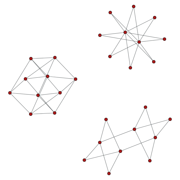
Figure 1: An example query to the Encyclopedia using specific invariant conditions. The command python viewer.py 10 -i is_bipartite 1 -i is_integral 1 -i is_eulerian 1 displays the three graphs that are simultaneously bipartite, integral and Eulerian with ten vertices.

Appendix A Invariant Descriptions

The invariant descriptions are broadly organized into sections of algebraic graph theory, topological graph theory, and invariants related to structure-like connectivity. Readers are instructed to look to standard references for more comprehensive definitions [28, 29, 30].

Algebraic Graph Theory

The adjacency matrix $A$ has the value at $A_{ij}$ equal to the number of edges joining vertex $i$ to $j$. For simple graphs, this is a $\{0,1\}$ matrix with zeros down the diagonal. The characteristic polynomial for a matrix is given by its eigenvalues, $\det(\lambda I-A)$. A sequence of eigenvalues $\lambda_{1},\lambda_{2},\ldots$ is called the spectrum. A graph is $integral$ if all the values of the adjacency spectrum are integral, $\lambda_{k}\in\mathbb{Z}$. A graph is $real$ if $\lambda_{k}\in\mathbb{R}$.

An independent vertex/edge set is a subset of vertices/edges of a graph such that no two vertices/edges in the subset share an edge/vertex. The maximal independent vertex set or independence number, is the cardinality of the largest independent vertex set. A graph is bipartite if there exists two disjoint independent subsets of the vertices whose union is $V$. The maximal independent edge set is the cardinality of the largest independent edge set. The total number of independent edges sets is sometimes referred to as the number of edge matchings, or the Hosoya index[31]. For graphs that are bounded in treewidth the Hosoya index is fixed-parameter tractable. In general however, the Hosoya index $\mathcal{\#P}$-complete[32].

The automorphism group is formed by all mappings of the vertices onto themselves which preserve isomorphism. The cardinality of this group is the automorphism number. Both nauty and BLISS [33, 14] can compute the automorphism group and the number.

The Tutte polynomial is a bivariate polynomial which encodes information about the graph’s connectedness. The polynomial $T_{g}(x,y)$ is defined via the recurrence relation, $T_{g}=T_{g-e}+T_{g/e}$ for any edge $e\in E$ that is not a loop or a bridge. Here $g-e$ denotes edge removal, $g/e$ denotes edge contraction and a bridge is an edge whose removal disconnects the graph. A graph with only $i$ loops and $j$ bridges has the base case of $T_{g}(x,y)=x^{i}y^{j}$. The chromatic polynomial is a specialization of the Tutte polynomial

$$P_{g}(k)=(-1)^{|V|-c}k^{c}T_{g}(1-k,0)$$ (4)

where $c$ is the number of connected components of the graph. The chromatic polynomial $P_{g}(k)$ gives the number of proper $k$-colorings on a graph. A proper $k$-coloring of a graph is an assignment of $k$ colors to each vertex so that no two adjacent vertices have the same color. The chromatic number $\chi(g)$, is the smallest non-zero $k$ such that $P_{g}(k)>0$.

The fractional coloring number is motivated by the chromatic number. A graph is $a:b$ colorable if each vertex is assigned $b$ colors out of a palette of $a$ total colors such that the coloring of each adjacent vertex is disjoint. The smallest $a$ such that the graph can be assigned to $b$ colors is the $b$-fold chromatic number and is denoted by $\chi_{b}(g)$. Note that the standard chromatic number is $\chi(g){}=\chi_{1}(g)$. The fractional coloring number is defined to be

$$\chi_{f}(g)=\lim_{b\rightarrow\infty}\frac{\chi_{b}(g)}{b}=\inf_{b}\frac{\chi_{b}(g)}{b}$$ (5)

Not only does the limit exist, but $\chi_{f}(g)\in\mathbb{Q}$[34]. The integral chromatic number need not be equal to its fractional counter part, in fact $\chi_{f}(g)\leq\chi(g)$. If the equality does not hold, we say the graph has a fractional chromatic gap. Additionally, we can formulate $\chi_{f}(g)$ as a solution to a linear program. Let $I(g)$ be the set of all independent vertex sets and $I(g,v)$ be the set of independent vertex sets that contain vertex $v$. Define a system of non-negative variables $v_{i}$. Now $\chi_{f}(g)$ is the minimum of $\sum_{I\in I(g)}v_{i}$ subject to the constraints $\sum_{I\in I(g,x)}v_{i}\geq 1$ on each $v_{i}$.

Topological Graph Theory

The crossing number is the minimum possible number of edge crossings for an embedding of the graph in a plane. A graph is planar if the crossing number is zero, in other words, a graph is planar if it admits an embedding in the plane with no overlapping edges. A graph is toroidal if the crossing number is one. The genus is the minimum number of edges that must be added to a graph to make it planar. Due to a lack of freely available algorithms, planarity is the only embedding currently considered.

Connectivity, Cycles and Subgraphs

The degree of vertex $k$ is the number of edges incident to the vertex, $d(v_{k})=\sum_{j}A_{kj}$. The degree sequence is formed by listing the vertex degrees in descending order, and the number of distinct degree sequences for graphs for simple connected graphs is OEIS A007721. The degree matrix is a diagonal matrix defined by the degree sequence. The Laplacian matrix is the difference of the diagonal matrix and the adjacency matrix. The Laplacian polynomial is the characteristic polynomial of the Laplacian matrix. For connected graphs the spectrum of the Laplacian matrix is real and $\lambda_{i}\leq 0,\lambda_{0}=0$. The second-largest eigenvalue is called the spectral gap.

Let $D$ denote the graph distance matrix, where $D_{ij}$ is the shortest path (geodesic) from vertex $i$ to $j$. A graph is connected if there is a path between all pairs of vertices. If there is no path between vertices $i$ and $j$, $D_{ij}=\infty$. By construction, all distances in connected graphs are finite. The eccentricity of a vertex $k$ is the maximum value of $D_{kj}$ for all $j$. The radius/diameter is the minimum/maximum value of eccentricity for all vertices.

A $k$-regular graph is one in which every vertex has degree $k$. A regular graph is strongly regular, if there exist integers $a$ and $b$ such that any two adjacent vertices have $a$ neighbors in common and any two non-adjacent vertices have $b$ neighbors in common. A graph is distance regular if two conditions are met. First, for all pairs of vertices $v,w$ and any pair of integers $i,j=0,1,\ldots,d$ where $d$ is the graph diameter, the number of vertices from $v$ at a distance $i$ and the number of vertices from $w$ at a distance $j$ depend only on $i,j$. Secondly, if the distance between $v$ and $w$ is independent of the choice of $v$ and $w$[35].

A circuit is a path that begins and ends at the same vertex. A graph is Hamiltonian/Eulerian if there is a circuit that visits each vertex/edge exactly once.

A vertex is an articulation point if its removal disconnects the graph. The vertex/edge connectivity of a graph is the minimum number of vertices/edges needed to disconnect the graph. A vertex joined to only a single edge is an end point.

The cycle space of a graph is the set of all of its Eulerian subgraphs, where every member can be constructed as the symmetric difference of members of the cycle basis. A tree is an acyclic connected graph whose cycle basis is the empty set. The length of the shortest/longest cycle in a graph is its girth/circumference. Trees are defined to have infinite girth and circumference. Due to technical limitations we record this value as a zero which is unambiguous for connected loopless graphs. A chord of a cycle is an edge with one vertex belonging to the cycle and one edge outside of the cycle. In a chordal graph, all cycles of order four or more have a cycle chord.

A vertex subgraph or simply a subgraph, is a subset of vertices and the edges which are common to all members of this subset. Let $s(g,h)$ equal the number of vertex sets that form subgraphs of $h$ in $g$. The maximum clique number is the largest non-zero value of $s(g,K_{n})$, where $K_{n}$ is the complete graph on $n$ vertices. A graph is triangle free or square free if $s(g,C_{3})=0$ or $s(g,C_{4})=0$ respectively, where $C_{n}$ is the cycle graph on $n$ vertices. In addition, we have checked for the subgraphs $K_{4},K_{5},C_{5},C_{6}$ and several named graphs. Illustrated below from left-to-right are the the bull graph $B_{5}{}$, the bowtie graph $\bowtie{}$, the open-bowtie graph $\rtimes{}$, and the diamond graph $D_{4}{}$.

Appendix B Submitted sequences

The sequences that were already present in the OEIS but extended by this project are listed in Section B.1. The distinct sequences were those formed by considering the number of unique values possible at a fixed order and are listed in Section B.2. Sequences involving a single invariant, the primary sequences, are listed in Section B.3. The secondary sequences involve two invariants and are listed in Section B.4.

Each sequence was hand-checked against the OEIS. We validated that either the sequence was unique or the invariant description matched the sequence found. We reiterate that all results shown are for simple, connected graphs. For some invariants the definition may be ambiguous for small orders. When possible, we tried to refer to conventions found in the literature and the OEIS for these cases. For brevity the symbols describing the invariants are shown below.

Invariant symbol	Description
$|\text{Aut}(g)|$	Automorphism group size
$\chi(g)$	Chromatic number
$\kappa_{V}(g)$, $\kappa_{E}(g)$	vertex/edge connectivity
$\text{dia}(g),\text{girth}(g)$	diameter, girth
$a(g)$	number of articulation points
$\alpha_{V}(g),\alpha_{E}(g)$	size of maximal independent vertex/edge set
$s{}(g,h)$	number of subgraphs of $h$ in $g$
$T,H,E,I,I^{*}$	properties: tree, Hamiltonian, Eulerian, integral, real
$R,R^{*},D,B$	properties: regular, strongly regular, distance regular, bipartite
$C,X$	properties: chordal, chromatic gap

B.1 Extended sequences

OEIS	Invariant	Sequence: $S_{1},S_{2},\ldots,S_{10}$, terms in $(\cdot)$ were added by this project
A086216	$\kappa_{V}(g)>3$	0	0	0	0	1	4	25	384	14480	(1211735)
A086217	$\kappa_{V}(g)>4$	0	0	0	0	0	1	4	39	1051	(102630)
A052446	$\kappa_{E}(g)=2$	0	1	1	3	10	52	351	3714	63638	(1912203)
A052447	$\kappa_{E}(g)=3$	0	0	1	2	8	41	352	(4820)	(113256)	(4602039)
A052448	$\kappa_{E}(g)=4$	0	0	0	1	2	15	121	(2159)	(68715)	(3952378)
A088741	$R^{*}(g)=1$	1	1	1	2	2	3	1	3	3	(5)

B.2 Distinct sequences

OEIS	Invariant	Sequence: $S_{1},S_{2},\ldots,S_{10}$
A245881	Tutte poly	1	1	2	5	16	73	532	7245	192605	9717156
A245883	chromatic poly	1	1	2	5	14	50	231	1650	21121	584432
A245880	characteristic poly	1	1	2	6	21	111	821	10423	236064	10375796
A245882	Laplacian poly	1	1	2	6	21	110	793	10251	239307	10985229
A245879	fractional chromatic	1	1	2	3	5	7	11	17	29	50

B.3 Primary sequences

OEIS	Invariant	Sequence: $S_{1},S_{2},\ldots,S_{10}$
A241454	$|\text{Aut}(g)|=2$	0	1	1	2	9	37	317	4098	84602	2933996
A241455	$|\text{Aut}(g)|=4$	0	0	0	1	3	28	198	1971	29047	672516
A241456	$|\text{Aut}(g)|=6$	0	0	1	1	1	7	31	221	3025	68033
A241457	$|\text{Aut}(g)|=8$	0	0	0	1	2	9	55	499	6017	107312
A241458	$|\text{Aut}(g)|=10$	0	0	0	0	1	1	1	3	13	123
A241459	$|\text{Aut}(g)|=12$	0	0	0	0	3	10	51	356	3395	49862
A241460	$|\text{Aut}(g)|=14$	0	0	0	0	0	0	2	2	2	6
A241461	$|\text{Aut}(g)|=16$	0	0	0	0	0	3	10	123	992	14026
A241462	$|\text{Aut}(g)|=20$	0	0	0	0	0	0	2	6	29	199
A241463	$|\text{Aut}(g)|=24$	0	0	0	1	1	1	14	118	1247	17191
A241464	$|\text{Aut}(g)|=36$	0	0	0	0	0	1	3	16	132	1341
A241465	$|\text{Aut}(g)|=48$	0	0	0	0	0	4	14	65	504	5215
A241466	$|\text{Aut}(g)|=72$	0	0	0	0	0	1	2	16	124	1070
A241467	$|\text{Aut}(g)|=120$	0	0	0	0	1	1	1	5	21	211
A241468	$|\text{Aut}(g)|=144$	0	0	0	0	0	0	3	12	51	477
A241469	$|\text{Aut}(g)|=240$	0	0	0	0	0	0	3	8	51	336
A241470	$|\text{Aut}(g)|=720$	0	0	0	0	0	1	1	4	13	60
A241471	$|\text{Aut}(g)|=5040$	0	0	0	0	0	0	1	1	1	5
A241702	$\chi(g)=7$	0	0	0	0	0	0	1	6	110	4125
A241703	$\kappa_{E}(g)=4$	0	0	0	0	1	3	25	378	14306	1141575
A241704	$\kappa_{E}(g)=5$	0	0	0	0	0	1	3	41	1095	104829
A241705	$\kappa_{E}(g)=6$	0	0	0	0	0	0	1	4	65	3441
A241706	$\text{dia}(g)=2$	0	0	1	4	14	59	373	4154	91518	4116896
A241707	$\text{dia}(g)=3$	0	0	0	1	5	43	387	5797	148229	6959721
A241708	$\text{dia}(g)=4$	0	0	0	0	1	8	82	1027	19320	598913
A241709	$\text{dia}(g)=5$	0	0	0	0	0	1	9	125	1818	37856
A241710	$\text{dia}(g)=6$	0	0	0	0	0	0	1	12	180	2928
A241711	$\text{girth}(g)=3$	0	0	1	3	15	93	792	10833	259420	11704309
A241712	$\text{girth}(g)=4$	0	0	0	1	2	11	43	234	1498	11451
A241713	$\text{girth}(g)=5$	0	0	0	0	1	1	5	18	82	539
A241714	$\text{girth}(g)=6$	0	0	0	0	0	1	1	7	25	137
A241715	$\text{girth}(g)=7$	0	0	0	0	0	0	1	1	6	20
A241767	$a(g)=1$	0	0	1	2	7	33	244	2792	52448	1690206
A241768	$a(g)=2$	0	0	0	1	3	17	101	890	11468	239728
A241769	$a(g)=3$	0	0	0	0	1	5	32	242	2461	35839
A241770	$a(g)=4$	0	0	0	0	0	1	7	60	527	6056
A241771	$a(g)=5$	0	0	0	0	0	0	1	9	97	1029
A241782	$s{}(g,K_{5})=0$	1	1	2	6	20	107	802	10252	232850	9905775
A241784	$s{}(g,C_{5})=0$	1	1	2	6	13	44	144	577	2457	12499
A242790	$s{}(g,D_{4})=0$	1	1	2	4	11	39	165	967	7684	87012
A242792	$s{}(g,\rtimes)=0$	1	1	2	6	15	60	273	1769	14836	174111
A242791	$s{}(g,\bowtie)=0$	1	1	2	6	11	34	98	408	1957	12740
A243243	$s{}(g,C_{4})>0$	0	0	0	3	13	93	796	10931	260340	11713182
A243246	$s{}(g,C_{5})>0$	0	0	0	0	8	68	709	10540	258623	11704072
A243245	$s{}(g,K_{3})>0$	0	0	1	3	15	93	794	10850	259700	11706739
A243244	$s{}(g,K_{4})>0$	0	0	0	1	4	30	317	5511	165165	8932499
A243242	$s{}(g,K_{5})>0$	0	0	0	0	1	5	51	865	28230	1810796
A243250	$s{}(g,D_{4})>0$	0	0	0	2	10	73	688	10150	253396	11629559
A243248	$s{}(g,B_{5})>0$	0	0	0	0	12	86	773	10777	259390	11705139
A243249	$s{}(g,\rtimes)>0$	0	0	0	0	6	52	580	9348	246244	11542460
A243247	$s{}(g,\bowtie)>0$	0	0	0	0	10	78	755	10709	259123	11703831
A241814	${D}(g)=1$	1	1	1	2	2	4	2	5	4	7
A241839	${R}(g)=0$	1	0	1	4	19	107	849	11100	261058	11716404
A241840	${D}(g)=0$	0	0	1	4	19	108	851	11112	261076	11716564
A241841	${T}(g)=0$	0	0	1	4	18	106	842	11094	261033	11716465
A241842	${I}(g)=0$	0	0	1	4	18	106	846	11095	261056	11716488
A241843	${C}(g)=0$	0	0	0	1	6	54	581	9503	249169	11607032
A242952	${I^{*}}(g)=1$	1	1	1	3	11	54	539	7319	209471	10000304
A242953	${I^{*}}(g)=0$	0	0	1	3	10	58	314	3798	51609	1716267
A243241	${R^{*}}(g)=0$	0	0	1	4	19	109	852	11114	261077	11716566
A243251	${X}(g)=1$	0	0	0	0	1	3	33	496	16464	969293
A243252	${X}(g)=0$	1	1	2	6	20	109	820	10621	244616	10747278
A243781	$\alpha_{V}(g)=2$	0	0	1	4	11	34	103	405	1892	12166
A243782	$\alpha_{V}(g)=3$	0	0	0	1	8	63	524	5863	100702	2880002
A243783	$\alpha_{V}(g)=4$	0	0	0	0	1	13	205	4308	135563	7161399
A243784	$\alpha_{V}(g)=5$	0	0	0	0	0	1	19	513	21782	1576634
A243800	$\alpha_{E}(g)=2$	0	0	0	5	20	16	22	29	37	46
A243801	$\alpha_{E}(g)=3$	0	0	0	0	0	95	830	790	1479	2625

B.4 Secondary sequences

OEIS	Invariant		Sequence: $S_{1},S_{2},\ldots,S_{10}$
A243270	${H}(g)=1$,	${B}(g)=1$	1	0	0	1	0	4	0	24	0	473
A243271	${H}(g)=1$,	${D}(g)=1$	1	0	1	2	2	4	2	5	4	6
A243272	${H}(g)=1$,	${E}(g)=1$	1	0	1	1	2	5	21	120	1312	26525
A243273	${H}(g)=1$,	${I}(g)=0$	0	0	0	1	7	43	379	6185	177071	9305068
A243274	${H}(g)=1$,	${I}(g)=1$	1	0	1	2	1	5	4	11	12	50
A243275	${H}(g)=1$,	$s{}(g,K_{3})=0$	1	0	0	1	1	4	5	35	130	1293
A243276	${H}(g)=1$,	$s{}(g,K_{4})=0$	1	0	1	2	5	29	188	2481	52499	1857651
A243319	${B}(g)=1$,	${D}(g)=1$	1	1	0	1	0	2	0	3	0	3
A243320	${B}(g)=1$,	${E}(g)=1$	1	0	0	1	0	2	1	6	7	29
A243321	${B}(g)=1$,	${P}(g)=1$	1	1	1	3	5	16	41	158	582	2749
A243322	${D}(g)=1$,	${E}(g)=1$	1	0	1	1	2	2	2	3	4	4
A243323	${I}(g)=0$,	${B}(g)=1$	0	0	1	2	4	14	43	179	730	4019
A243324	${I}(g)=0$,	${E}(g)=1$	0	0	0	0	2	6	33	180	1773	31006
A243325	${I}(g)=0$,	${P}(g)=1$	0	0	1	4	18	95	642	5962	71876	1052786
A243326	${I}(g)=0$,	$s{}(g,K_{3})=0$	0	0	1	2	5	16	58	264	1380	9818
A243327	${I}(g)=0$,	$s{}(g,K_{4})=0$	0	0	1	4	15	77	531	5597	95900	2784034
A243328	${I}(g)=1$,	${B}(g)=1$	1	1	0	1	1	3	1	3	0	13
A243329	${I}(g)=1$,	${D}(g)=1$	1	1	1	2	1	4	1	4	3	6
A243330	${I}(g)=1$,	${E}(g)=1$	1	0	1	1	2	2	4	4	9	20
A243331	${I}(g)=1$,	${P}(g)=1$	1	1	1	2	2	4	4	12	9	19
A243332	${I}(g)=1$,	$s{}(g,K_{3})=0$	1	1	0	1	1	3	1	3	0	14
A243333	${I}(g)=1$,	$s{}(g,K_{4})=0$	1	1	1	1	2	5	5	9	15	38
A243334	$s{}(g,K_{3})=0$,	${D}(g)=1$	1	1	0	1	1	2	1	3	1	4
A243335	$s{}(g,K_{3})=0$,	${E}(g)=1$	1	0	0	1	1	2	3	8	19	62
A243336	$s{}(g,K_{4})=0$,	${E}(g)=1$	1	0	1	1	3	6	22	93	656	7484
A243337	$s{}(g,K_{4})=0$,	${P}(g)=1$	1	1	2	5	17	79	478	4123	46666	648758
A243338	${T}(g)=1$,	${I}(g)=0$	0	0	1	2	2	5	10	23	47	105
A243339	$s{}(g,K_{4})=0$,	${D}(g)=1$	1	1	1	1	1	3	1	3	3	4
A243545	${H}(g)=1$,	$s{}(g,\rtimes)=0$	1	0	1	3	3	14	50	390	3627	52858
A243546	$s{}(g,\rtimes)=0$,	${D}(g)=1$	1	1	1	2	1	2	1	3	1	4
A243547	$s{}(g,\rtimes)=0$,	${E}(g)=1$	1	0	1	1	2	4	8	35	115	629
A243548	$s{}(g,\rtimes)=0$,	${I}(g)=1$	1	1	1	2	2	4	1	8	1	19
A243549	$s{}(g,\rtimes)=0$,	${I}(g)=0$	0	0	1	4	13	56	272	1761	14835	174092
A243550	$s{}(g,\rtimes)=0$,	${P}(g)=1$	1	1	2	6	15	58	255	1510	10766	94109
A243551	$s{}(g,\rtimes)=0$,	$s{}(g,K_{4})=0$	1	1	2	5	14	56	256	1656	13952	163878
A243552	$s{}(g,\rtimes)=0$,	$s{}(g,B_{5})=0$	1	1	2	6	8	25	77	333	1668	11355
A243553	${H}(g)=1$,	$s{}(g,B_{5})=0$	1	0	1	3	1	4	5	35	130	1293
A243554	$s{}(g,B_{5})=0$,	${D}(g)=1$	1	1	1	2	1	2	1	3	1	4
A243555	$s{}(g,B_{5})=0$,	${E}(g)=1$	1	0	1	1	2	3	5	14	30	95
A243556	$s{}(g,B_{5})=0$,	${I}(g)=1$	1	1	1	2	1	3	2	3	0	14
A243557	$s{}(g,B_{5})=0$,	${I}(g)=0$	0	0	1	4	8	23	78	337	1690	11418
A243558	$s{}(g,B_{5})=0$,	${P}(g)=1$	1	1	2	6	9	25	76	302	1360	7606
A243559	$s{}(g,B_{5})=0$,	$s{}(g,K_{4})=0$	1	1	2	5	9	26	80	340	1690	11432
A243560	${H}(g)=1$,	$s{}(g,D_{4})=0$	1	0	1	1	2	9	27	190	1750	25658
A243561	$s{}(g,D_{4})=0$,	${D}(g)=1$	1	1	1	1	1	2	1	3	2	4
A243562	$s{}(g,D_{4})=0$,	${E}(g)=1$	1	0	1	1	2	3	8	21	79	334
A243563	$s{}(g,D_{4})=0$,	${I}(g)=0$	0	0	1	3	10	35	162	964	7682	86994
A243564	$s{}(g,D_{4})=0$,	${I}(g)=1$	1	1	1	1	1	4	3	3	2	18
A243565	$s{}(g,D_{4})=0$,	${P}(g)=1$	1	1	2	4	11	38	159	882	6242	55316
A243566	$s{}(g,D_{4})=0$,	$s{}(g,K_{4})=0$	1	1	2	4	11	39	165	967	7684	87012
A243567	$s{}(g,D_{4})=0$,	$s{}(g,\rtimes)=0$	1	1	2	4	10	36	141	784	5626	56249
A243568	$s{}(g,D_{4})=0$,	$s{}(g,B_{5})=0$	1	1	2	4	9	26	80	340	1690	11432
A243789	$s{}(g,\bowtie)=0$,	$s{}(g,D_{4})=0$	1	1	2	4	9	30	89	379	1864	12365
A243790	$s{}(g,\bowtie)=0$,	${H}(g)=1$	1	0	1	3	3	9	13	59	203	1651
A243791	$s{}(g,\bowtie)=0$,	${E}(g)=1$	1	0	1	1	1	2	3	8	19	62
A243792	$s{}(g,\bowtie)=0$,	${I}(g)=1$	1	1	1	2	1	4	1	3	0	15
A243783	$s{}(g,\bowtie)=0$,	${I}(g)=0$	0	0	1	4	10	30	97	405	1957	12725
A243794	$s{}(g,\bowtie)=0$,	${P}(g)=1$	1	1	2	6	11	33	94	370	1627	8895
A243795	$s{}(g,\bowtie)=0$,	$s{}(g,B_{5})=0$	1	1	2	6	7	22	65	285	1442	10106
A243253	${C}(g)=1$,	${E}(g)=1$	1	0	1	0	3	2	13	18	116	366
A243785	${C}(g)=1$,	${I}(g)=0$	0	0	1	4	12	56	267	1605	11909	109525
A243786	${C}(g)=1$,	${I}(g)=1$	1	1	1	1	3	2	5	9	2	14
A243787	${C}(g)=1$,	${P}(g)=1$	1	1	2	5	14	52	228	1209	7463	52520
A243788	${C}(g)=1$,	$s{}(g,K_{4})=0$	1	1	2	4	11	35	124	500	2224	10640
A243796	${H}(g)=1$,	${C}(g)=1$	1	0	1	2	4	15	58	360	2793	28761
A243797	$s{}(g,\rtimes)=0$,	${C}(g)=1$	1	1	2	5	10	27	70	206	613	1942
A243798	$s{}(g,B_{5})=0$,	${C}(g)=1$	1	1	2	5	6	12	25	55	126	304
A243799	$s{}(g,\bowtie)=0$,	${C}(g)=1$	1	1	2	5	6	13	25	58	130	316

References

- [1] Ronald C Read and Robin J Wilson. An Atlas of Graphs. Clarendon Press, 1998.
- [2] Massimo De Santo, Pasquale Foggia, Carlo Sansone, and Mario Vento. A large database of graphs and its use for benchmarking graph isomorphism algorithms. Pattern Recognition Letters, 24(8):1067–1079, 2003.
- [3] Gunnar Brinkmann, Kris Coolsaet, Jan Goedgebeur, and Hadrien Mélot. House of graphs: A database of interesting graphs. Discrete Applied Mathematics, 161(1):311–314, 2013. http://hog.grinvin.org/.
- [4] Harry E Pence and Antony Williams. Chemspider: An online chemical information resource. Journal of Chemical Education, 87(11):1123–1124, 2010. http://www.chemspider.com.
- [5] Hin Hark Gan, Daniela Fera, Julie Zorn, Nahum Shiffeldrim, Michael Tang, Uri Laserson, Namhee Kim, and Tamar Schlick. Rag: Rna-as-graphs database—concepts, analysis, and features. Bioinformatics, 20(8):1285–1291, 2004. http://www.biomath.nyu.edu/?q=rag/home.
- [6] Christian Laing, Segun Jung, Namhee Kim, Shereef Elmetwaly, Mai Zahran, and Tamar Schlick. Predicting helical topologies in rna junctions as tree graphs. PloS one, 8(8):e71947, 2013.
- [7] Julian J. McAuley and Jure Leskovec. Discovering social circles in ego networks. TKDD, 8(1):4, 2014.
- [8] Ulrik Brandes, Patrick Kenis, Jürgen Lerner, and Denise van Raaij. Network analysis of collaboration structure in wikipedia. In Proceedings of the 18th International Conference on World Wide Web, WWW ’09, pages 731–740, New York, NY, USA, 2009. ACM.
- [9] Gal Oestreicher-Singer and Arun Sundararajan. Linking Network Structure to Ecommerce Demand: Theory and Evidence from Amazon.com’s Copurchase Network. 2006.
- [10] Hadrien Mélot. Facet defining inequalities among graph invariants: the system GraPHedron. Discrete Applied Mathematics, 156(10):1875–1891, 2008.
- [11] Travis Hoppe and Anna Petrone. Simple connected graph invariants up to order ten. Aug 2014. http://dx.doi.org/10.5281/zenodo.11280.
- [12] Travis Hoppe and Anna Petrone. Encyclopedia of finite graphs. Aug 2014. http://dx.doi.org/10.5281/zenodo.11304.
- [13] Neil JA Sloane et al. The on-line encyclopedia of integer sequences, 2003. https://oeis.org/.
- [14] Brendan D McKay and Adolfo Piperno. Practical graph isomorphism, ii. Journal of Symbolic Computation, 60:94–112, 2014.
- [15] Markus Meringer. Fast generation of regular graphs and construction of cages. Journal of Graph Theory, 30(2):137–146, 1999.
- [16] Gunnar Brinkmann. Fast generation of cubic graphs. Journal of Graph Theory, 23(2):139–149, 1996.
- [17] Gunnar Brinkmann, Jan Goedgebeur, Jonas Hägglund, and Klas Markström. Generation and properties of snarks. Journal of Combinatorial Theory, Series B, 103(4):468–488, 2013.
- [18] Joe Sawada. Generating rooted and free plane trees. ACM Transactions on Algorithms, 2(1):1–13, 2006.
- [19] Stephan Brandt, Gunnar Brinkmann, and Thomas Harmuth. The generation of maximal triangle-free graphs. Graphs and Combinatorics, 16(2):149–157, 2000.
- [20] Aric A. Hagberg, Daniel A. Schult, and Pieter J. Swart. Exploring network structure, dynamics, and function using networkx. In Proceedings of the 7th Python in Science Conference, pages 11–15, 2008. Software version: 1.9, https://networkx.github.io/.
- [21] Tiago de Paula Peixoto. Graph-Tool efficient network analysis. http://graph-tool.skewed.de, 2014. Software version: 2.2.31.
- [22] Stuart Mitchell, Michael O’Sullivan, and Iain Dunning. Pulp: a linear programming toolkit for python. 2011.
- [23] Paul Erdős. Graph theory and probability. Canadian Journal of Mathematics, 11:34–38, 1959.
- [24] Brendan McKay. Combinatorial data. http://cs.anu.edu.au/~bdm/data/.
- [25] Gordon Royle. Small graphs. http://staffhome.ecm.uwa.edu.au/~00013890/remote/graphs/.
- [26] Markus Meringer. Regular graphs. http://www.mathe2.uni-bayreuth.de/markus/reggraphs.html.
- [27] Nicolas Beldiceanu, Mats Carlsson, and Jean-Xavier Rampon. Global constraint catalog. SICS Research Report, 2005.
- [28] Reinhard Diestel. Graph theory. Springer, Heidelberg New York, 2010.
- [29] J. A. Bondy. Graph theory. Springer, New York, 2008.
- [30] Béla Bollobás. Modern graph theory. Springer, New York, 1998.
- [31] Haruo Hosoya. Topological index. a newly proposed quantity characterizing the topological nature of structural isomers of saturated hydrocarbons. Bull. Chem. Soc. Jpn, 44(9):2332–2339, 1971.
- [32] Mark Jerrum. Two-dimensional monomer-dimer systems are computationally intractable. Journal of Statistical Physics, 48(1-2):121–134, 1987.
- [33] Tommi A Junttila and Petteri Kaski. Engineering an efficient canonical labeling tool for large and sparse graphs. In ALENEX, volume 7, pages 135–149. SIAM, 2007.
- [34] Edward R Scheinerman and Daniel H Ullman. Fractional graph theory: a rational approach to the theory of graphs. Courier Dover Publications, 2011.
- [35] Andries E Brouwer and Willem H Haemers. Distance-regular graphs. Springer, 2012.