Classification of wave regimes in excitable systems with linear cross-diffusion

Abstract

We consider principal properties of various wave regimes in two selected excitable systems with linear cross-diffusion in one spatial dimension observed at different parameter values. This includes fixed-shape propagating waves, envelope waves, multi-envelope waves, and intermediate regimes appearing as waves propagating fixed-shape most of the time but undergoing restructuring from time to time. Depending on parameters, most of these regimes can be with and without the “quasi-soliton” property of reflection of boundaries and penetration through each other. We also present some examples of behaviour of envelope quasi-solitons in two spatial dimensions.

I Introduction

The progress in the study of self-organization phenomena in physical, chemical and biological systems is dependent on study of generation, propagation and interaction of nonlinear waves in spatially distributed active, e.g. excitable, systems with diffusion Merzhanov and Rumanov (1999). An important general property of such systems is their ability to generate and conduct self-supported strongly nonlinear waves of the change of state of the medium. The shape and speed of such waves in the established regime does not depend on initial and boundary conditions and is fully determined by the medium parameters. Until recently the results concerning such systems have been focused on systems “reaction+diffusion” with a diagonal diffusivity matrix, e.g. for two reacting components,

$$\frac{\partial u}{\partial t}=f(u,v)+D_{u}\nabla^{2}{u},\quad\frac{\partial v}{\partial t}=g(u,v)+D_{v}\nabla^{2}{v},$$ (1)

with non-negative diffusivities $D_{u}\geq 0$, $D_{v}\geq 0$, $D_{u}+D_{v}>0$. However, a number of applications motivate consideration of a more generic class of reaction-diffusion systems, with non-diagonal elements of the diffusivity matrix (“cross-diffusion”), which can produce a number of unusual patterns and wave regimes, see e.g. a review Vanag and Epstein (2009). In this paper we concentrate on one subclass of such unusual wave regimes, which is associated with soliton-like interaction, i.e. penetration of waves upon impact with each other or reflection from non-flux boundaries. This is rather uncharacteristic of the waves in (1) with the exception of narrow parametric regions on the margins of the excitability Aslanidi and Mornev (1999). However, in systems with cross-diffusion, such “quasi-soliton’ behaviour can be observed in large parametric regions Tsyganov et al. (2003); Biktashev and Tsyganov (2005). These phenomena have been observed in numerical simulations of two-component excitable media with cross-diffusion, both in linear formulation, e.g.

$$\frac{\partial u}{\partial t}=f(u,v)+D_{u}\nabla^{2}{u}+h_{1}\nabla^{2}v,$$

$$\frac{\partial v}{\partial t}=g(u,v)+D_{v}\nabla^{2}{v}-h_{2}\nabla^{2}u,$$ (2)

and nonlinear, “taxis” formulation,

$$\frac{\partial u}{\partial t}=f(u,v)+D_{u}\nabla^{2}{u}+h_{1}\nabla\left(u\nabla{v}\right),$$

$$\frac{\partial v}{\partial t}=g(u,v)+D_{v}\nabla^{2}{v}-h_{2}\nabla\left(v\nabla{u}\right),$$ (3)

where $h_{1}\geq 0$, $h_{2}\geq 0$, $h_{1}+h_{2}>0$.

Quasi-solitons have similarities and differences with the classical solitons in conservative (fully integrable) systems. The already mentioned similarity is their ability to penetrate through each other and reflect from boundaries. The differences are:

• The amplitude and speed of a true soliton depend on initial conditions. For the quasi-soliton, the established amplitude and speed depend on the medium parameters.

• The amplitudes of the true solitons do not change after the impact. The dynamics of quasi-solitons on impact is often naturally seen as a temporary diminution of the amplitude with subsequent gradual recovery.

Recently we have demonstrated “envelope quasi-solitons” in one-dimensional systems with linear cross-diffusion (2) Biktashev and Tsyganov (2011), which share some phenomenology with envelope solitons in the nonlinear Schrödinger equation (NLS) for a complex field $w$ Malomed (2005),

$$i\frac{\partial w}{\partial t}+\nabla^{2}w+w|w|^{2}=0.$$ (4)

Namely, they have the form of spatiotemporal oscillations (“wavelets”’) with a smooth envelope, and the velocity of the individual wavelets (the phase velocity) is different from the velocity of the envelope (the group velocity). This may be serious evidence for some deep relationship between these phenomena from dissipative and conservative realms. The link in this relationship is cross-diffusion, which for NLS is revealed if is rewriten as a system for two real fields $u$ and $v$ via $w=u-iv$ of the form (2) with

$$h_{1}=h_{2}=1,\quad D_{u}=D_{v}=0,$$

$$f=u(u^{2}+v^{2}),\quad g=-v(u^{2}+v^{2}).$$

Note the signs of the cross-diffusion terms in the componentwise form of NLS and in (2).

Further investigation has revealed a great variety of the types of nonlinear waves in excitable cross-diffusion systems. In this paper we present some classification of the phenomenologies of such waves.

Our observations are made in two selected two-component kinetic models, supplemented with cross-diffusion, rather than self-diffusion terms; such terms may appear, say, in mechanical Cartwright et al. (1997), chemical Chung and Peacock-López (2007); Vanag and Epstein (2009), biological and ecological Tsyganov et al. (2007); Murray (2003) contexts. We note that the case of only cross-diffusion terms, with $D_{u}=D_{v}=0$, is special in that the spatial coupling is then not dissipative, and all the dissipation in the system is due to the kinetic terms. So, theoretically speaking, this case may present features that are not characteristic for more realistic models. In practice, however, these worries seem unfounded. Parametric studies done in the past Tsyganov et al. (2003, 2004) indicate that the role of the self-diffusion coefficients $D_{u}$, $D_{v}$ is not essential if they are small enough. Moreover, we have verified that the results presented below are robust in that respect, too. In other words, regimes observed for $D_{u}=D_{v}=0$ typically are qualitatively preserved, even if quantitatively modified, upon adding small $D_{u}$, $D_{v}$. So in this study we limit consideration to $D_{u}=D_{v}=0$ to reduce number of parameters and focus attention on effects of the cross-diffusion terms. Except where stated otherwise, the values of the cross-diffusion coefficients are $h_{1}=h_{2}=1$. We consider the FitzHugh-Nagumo (FHN) kinetics,

$$f=u(u-a)(1-u)-k_{1}v,\quad g=\varepsilon u,$$ (5)

for varied values of parameters $a$, $k_{1}$, and $\varepsilon$. As a specific example of a real-life system, we also consider the Lengyel-Epstein (LE) Lengyel and Epstein (1991) model of a chlorite-iodide-malonic acid-starch autocatalitic reaction system

$$f=A-u-\frac{4uv}{1+u^{2}},\quad g=B\left(u-\frac{uv}{1+u^{2}}\right).$$ (6)

for varied values of parameters $A$ and $B$.

II Methods

We simulate (2) in one spatial dimension for $x\in[0,L]$, $L\leq\infty$, with Neumann boundary conditions for both $u$ and $v$. We use first order time stepping, fully explicit in the reaction terms and fully implicit in the cross-diffusion terms, with a second-order central difference approximation for the spatial derivatives. Unless stated otherwise, we used steps $\Delta x=1/10$ and $\Delta t=1/5000$ for FHN kinetics (5) and $\Delta x=0.1$ and $\Delta t=1/1000$ for LE kinetics (6).

To simulate propagation “on an infinite line”, we did the simulations on a finite but sufficiently large $L$ (specified in each case), and instantanously translated the solution by $\delta x_{1}=30$ away from the boundary each time the pulse, as measured at the level $u=u_{*}$, where $u_{*}=0.1$ for FHN kinetics and $u_{*}=1.5$ for LE kinetics, approached the boundary to a distance smaller than $\delta x_{2}=100$, and filled in the new interval of $x$ values by extending the $u$ and $v$ variables at levels $u=u_{0}$, $v=v_{0}$, where $(u_{0},v_{0})$ is the resting state, $u_{0}=v_{0}=0$ for FHN kinetics and $u_{0}=A/5$, $v_{0}=1+A^{2}/25$ for LE kinetics.

Initial conditions were set as $u(x,0)=u_{0}+u_{s}\operatorname{\Theta}(\delta-x)$, $v(x,0)=v_{0}$, to initiate a wave starting from the left end of the domain. Here $\operatorname{\Theta}()$ is the Heaviside function, and the wave seed length was typically chosen as $\delta=2$ or $\delta=4$. The interval length $L$ was chosen sufficiently large, say for the system (2,5) it was typically at least $L=350$, to allow wave propagation unaffected by boundaries, for some significant time.

To characterize shape of the waves emerging in simulations and its evolution, we counted significant peaks (wavelets) in the solutions as the number $n$ of continuous intervals of $x$ where $u-u_{0}>0.1$. In some regimes, this number varied with time, as the shape of enveloped changed while propagating. We also measured the speed of individual wavelets as the speed of the fore ends of these intervals at short time intervals. To estimate the group velocity, we considered the fore edge of the foremost significant peak over a longer time interval, covering several oscillation periods.

To compare the oscillatory front of propagating waves to the linearized theory, we took the $v$-component of the given solution in the interval and selected the connected area in the $(x,t)$ plane where $|v(x,t)|<0.1$ ahead of the main wave. We numerically fitted this grid function $v(x,t)$ to (7) using Gnuplot implementation of Marquardt-Levenberg algorithm. The initial guess for parameters $C$, $\mu$, $c$, $k$, $x$, $\omega$ was done “by eye”. The fitting was initially on a small interval in time, smaller than the temporal period of the front oscillations, and then gradually extended to a long time interval, so that the result of one fitting was used as the initial guess for the next fitting.

III Results

III.1 Overview of wave types

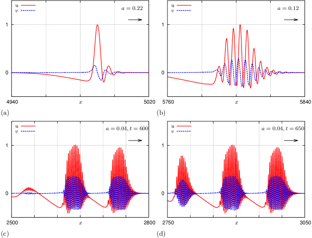
Figure 1: (color online) Three typical wave regimes in the cross-diffusion system (2,5) with $k_{1}=10$, $\varepsilon=0.01$ for different values of $a$. (a) Simple quasi-soliton, $a=0.22$. (b) Envelope quasi-soliton, $a=0.12$. (c,d) Multi-envelope qausi-soliton, $a=0.04$, at two different time moments.

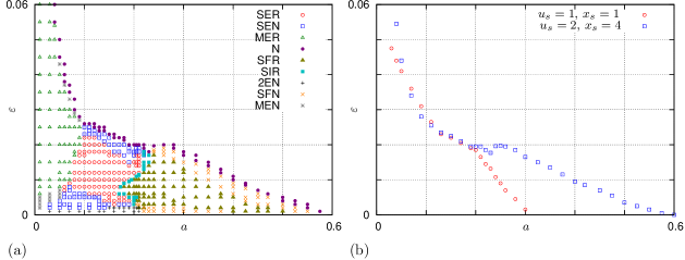
Figure 2: (a) The parametric regions corresponding to different wave regimes in (2,5) in the ($a,\varepsilon)$ plane at $k_{1}=10$, $x_{s}=4$, $u_{s}=2$. The abbreviations in the legend stand for various types of typical wave solutions: SER single envelope reflecting; SEN single envelope non-reflecting; MER multiple envelope reflecting; MEN multiple envelope non-reflecting; SFR single fixed-shape reflecting; SFN single fixed-shape non-reflecting; SIR single intermediate (between single shape and envelope) reflecting; 2EN envelope non-reflecting with separate envelopes at the front and at the back with non-oscillating plateau between them; N no propagation. See Supplementary Material epa for a movie. (b) Boundaries of the regimes of propagation and decay (of any waves) for different initial conditions.

Fig. 1 illustrates the three main types of waves in the excitable cross-diffusion system (2) with FHN kinetics (5). Fig. 2 explains why these are “main” types. It shows the regions in the parametric plane $(a,\varepsilon)$, and we see that the solutions shown in fig. 1 are represented by large parametric areas. Their common features are quasi-soliton interaction and oscillatory front, and the differences are in the propagation mode. A simple quasi-soliton (fig. 1(a), abbreviation SFR in fig. 2(a)) retains its shape as it propagates. A group, or envelope, quasi-soliton (fig. 1(b), abbreviation SER in fig. 2(a)) does not have a fixed shape; instead it has the form of spatiotemporal oscillations, whose envelope retains a fixed unimodal shape as it propagates. A multi-envelope quasi-soliton (fig. 1(c,d), abbreviation MER in fig. 2(a)) is shown at two time moments, to illustrate the dynamics of its formation. At first, the emerging solution looks like an envelope quasi-soliton; however after some time behind it forms another envelope quasi-soliton, then behind that one yet another, and so it continues. The interval of time between formation of new envelopes depends on the parameters, e.g. it becomes smaller for smaller values of $a$.

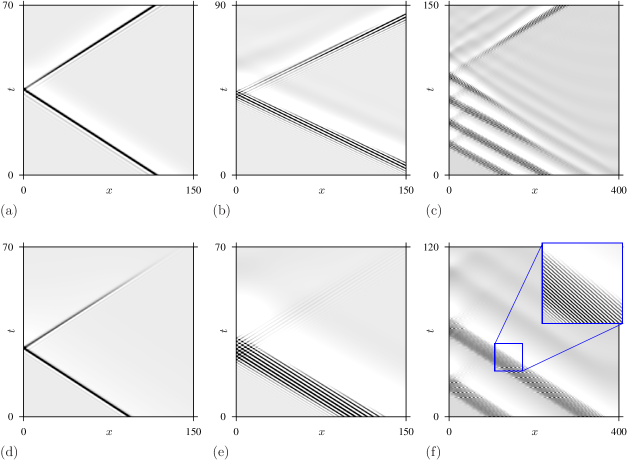
Figure 3: Density plots of impact episodes for selected regimes designated in fig. 2). (a) SFR: single fixed-shaped (“simple”) quasi-soliton, $a=0.22$, $\varepsilon=0.01$. (b) SER: single envelope quasi-soliton, $a=0.1$, $\varepsilon=0.01$. (c) MER: multiple envelope quasi-soliton, $a=0.02$, $\varepsilon=0.01$. In the panel, only the first reflected envelope has almost recovered within the view; other envelopes recover later. (d) SFN: single fixed-shape non-reflecting wave, $a=0.45$, $\varepsilon=0.004$. (e) SEN: single envelope non-reflecting wave, $a=0.1$, $\varepsilon=0.004$. (f) MEN: multiple envelope non-reflecting wave, $a=0.02$, $\varepsilon=0.004$. In (c) and (f), individual wavelets are not distinguishable at printing resolution so only the envelope is in fact seen; in (f) the fine structure of the wavelets is shown magnified in the inset. White corresponds to $u=-0.3$, black corresponds to $u=1$. Time reference point $t=0$ is chosen arbitrarily at the beginning of the selected episode; point $x=0$ corresponds to the left boundary of the interval. All simulations are done for $\Delta x=0.1$, $\Delta t=0.001$, $L=400$, $k_{1}=10$.

Each of the three types of quasi-solitons shown in fig. 1 has a counterpart type of solutions of similar propagation mode, but without the quasi-soliton property, i.e. not reflecting upon collision (abbreviations SFN, SEN, MEN in fig. 2(a)). Density plots of interaction of the three main types of quasi-solitons and their non-soliton counterparts are shown in fig. 3. Note that the non-soliton regimes do not show immediate annihilation upon the collision. Rather, the process looks like reflection with a decreased amplitude, and subsequent decay, see fig. 3(d-f).

Apart from the non-reflecting counterparts to the three main types, there are also “non-propagating” counterparts, all of which are denoted by N in fig. 2(a). These regimes correspond to waves that are in fact formed from the standard initial conditions, but then decay after some time. Naturally, the success of initiation of a propagating wave does in fact depend on the parameters of the initial conditions: fig. 2(b) shows how the region of single quasi-soliton differs for two different initial conditions. This is of course expectable for excitable kinetics.

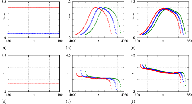
Figure 4: Dynamics of (a–c) amplitudes and (d–f) velocities of individual wavelets for the three types of quasi-solitons in (2,5) for $k_{1}=10$, $\varepsilon=0.01$. (a,d) Simple quasi-soliton, $a=0.22$, see fig. 1(a). (b,e) Envelope quasi-soliton, $a=0.12$, see fig. 1(b). (c,f) Multi-envelope quasi-solitons, $a=0.04$, see fig. 1(c,d).

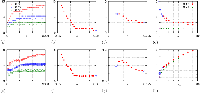
Figure 5: (a–d) Number of wavelets and (e–h) velocities of the envelope waves in transient and in established regimes. (a,e) The transients for $k_{1}=10$, $\varepsilon=0.01$ and three values $a=0.08$ (circles), $0.12$ (squares) and $0.16$ (triangles). (b,f) Established quantities as functions of parameter $a$ for fixed $k_{1}=10$, $\varepsilon=0.01$. (c,g) Established quantities as functions $\varepsilon$ for fixed $a=0.12$, $k_{1}=10$. (d,h) Established quantities as functions $k_{1}$ for fixed $\varepsilon=0.01$ and $a=0.12$ (circles) and $a=0.22$ (triangles). In (b–d) and (f–h), filled symbols designate quasi-soliton (reflecting) waves and open symbols designate non-reflecting waves.

The analysis of the dynamics of the wavelets and wavespeeds for the three main types of quasi-solitons, illustrated in figures 4 and 5, reveals:

• The amplitude and speed of the simple quasi-solitons do not change in time (fig. 4(a,d)).

• For the envelope and multi-envelope quasi-solitons, the amplitudes of individual wavelets during their lifetime first grow to a certain maximum and then decrease monotinically (fig. 4(b,c)). The speed of a wavelet (the phase velocity) is high at first, but the decreases non-monotonically (fig. 4(e,f)).

• In the process of establishment of an envelope quasi-soliton, the number of wavelets in it increases until saturation (fig. 5(a)), and so does the speed of the envelope (the group velocity) (fig. 5(e)).

• Fig. 5(b,f) shows that in simple quasi-solitons ($a>0.2$), the number of wavelets remains the same ($n=2$), and their speed remains approximately the same in that interval; whereas in envelope quasi-solitons ($a<0.2$), both the number of wavelets and their velocities increase with the decrease of $a$.

• Fig. 5(c,g) shows that increase of parameter $\varepsilon$ causes decrease of both the number of wavelets and of their speeds.

• Parameter $k_{1}$ also plays a significant role in definining the wave regime and its parameters (fig. 5(d,h)).

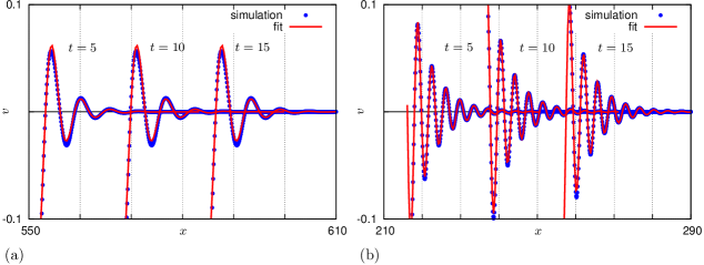
Figure 6: Profiles of established propagating waves at selected moments of time for $k_{1}=10$, $\varepsilon=0.01$, $L=\infty$. The origins of the $t$ and $x$ axes are chosen arbitrarily. (a) Simple quasi-soliton, $a=0.22$. (b) Envelope quasi-soliton, $a=0.12$.

The oscillatory character of the fronts of cross-diffusion waves both for simple quasi-solitons and for envelope quasi-solitons, which is apparent from numerical simulations, is easily confirmed by linearization of (2) around the resting state. The resting states in both FHN (5) and LE (6) kinetics are stable foci which already shows propensity to oscillations. Taking the solution of the linearized equation in the form

$$\left[\begin{array}[]{cc}u-u_{0}\\ v-v_{0}\end{array}\right]\approx\mathop{\mathrm{Re}}\left(C\mathbf{v}e^{-\mu(x-ct)}e^{i(kx-\omega t)}\right),$$ (7)

we need

$$\mathbf{A}(\lambda,\nu)\mathbf{v}=\mathbf{0},\quad\mathbf{v}\neq\mathbf{0},\quad\det\mathbf{A}=0,\\$$ (8)

where

$$\mathbf{A}=\left[\begin{array}[]{cc}-a-\lambda&-k_{1}+\nu^{2}\\ \varepsilon-\nu^{2}&-\lambda\end{array}\right],$$

$$\lambda=\mu c-i\omega,\;\nu=-\mu+ik.$$

Equation (8) imposes two constraints (for the real and imaginary parts of the determinant) on the four real quantities $\mu$, $c$, $k$ and $\omega$, so it is by far insufficient to determine the selection of these parameters, but this equality can be verified for the numerical simulations, in order to ensure that the observed oscillatory fronts are not a numerical artefact but a true property of the underlying partial differential equations. Hence we fitted selected simulations around the fronts with the dependence (7). The quality of the fitting is illustrated by two examples in fig. 6. The fitted parameters satisfied (8) with good accuracy; in both cases, they gave $|\det\mathbf{A}/(\operatorname{Tr}\mathbf{A})^{2}|<10^{-3}$.

Note that the approximation (7) makes explicit the concepts of wavelets (the oscillating factor $e^{i(kx-\omega t)}$), the phase velocity (the ratio $\omega/k$), the envelope (in this case the exponential shape $e^{-\mu(x-ct)}$) and the group velocity (the fitting parameter $c$). As expected, for the simple quasi-soliton shown in fig. 6(a) the fitted group and phase velocities coincided within the precision of fitting ($|c-\omega/k|<10^{-5}$). For the envelope quasi-soliton shown in fig. 6(b) they were significantly different: $c\approx 4.077$, $\omega/k\approx 3.586$.

III.2 Multi-envelope quasi-solitons

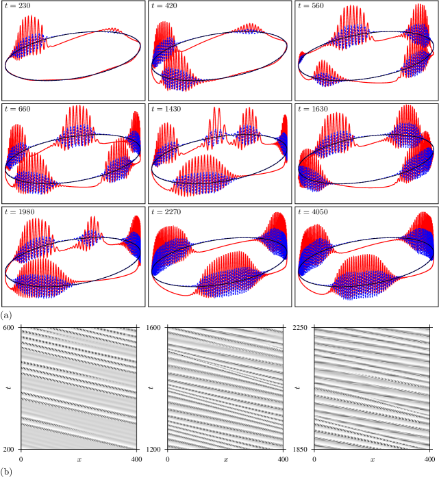
Figure 7: Formation and evolution of a multi-envelope quasi-soliton regime on a circle (1D cable with periodic boundary conditions), for $a=0.03$, $k_{1}=10$, $\varepsilon=0.01$. (a) Snapshots of the profiles at selected moments of time. The waves and wavelets propagate counterclockwise. (b) Density plots of the $u$ component of the solution for selected time intervals; white corresponds to $u_{\min}=-0.2$, black corresponds to $u_{\max}=1$ corresponds to black. See also the movie in the Supplementary Materials epa .

We use the term multiplying envelope quasi-solitons (MEQS) to concisely designate spontaneously multiplying envelope quasi-solitons. The process of self-multiplication leads to eventually filling the whole domain, behind the leading edge of the first group, with what appears as a train of envelope quasi-solitons, i.e. a hierarchical, quasi-periodic regime. This is illustrated in fig. 7(a) for periodic boundary conditions, the setting that eliminates the “leading edge” complication mentioned above. One envelope quasi-soliton (EQS) produced by the standard initial conditions develops an instability at its tail, leading to generation of the second EQS ($t=230$). The system of two EQSs generates a third ($t=420$). After forming of a system of five EQSs ($t=600$), the inverse transition happens, from five to four envelopes ($t=1430$, $t=1630$), and then from four to three envelopes ($t=1980$, $t=2270$), leading to an established, persistent state of three envelopes ($t=4050$). The same process is represented also as a density plot in fig. 7(b).

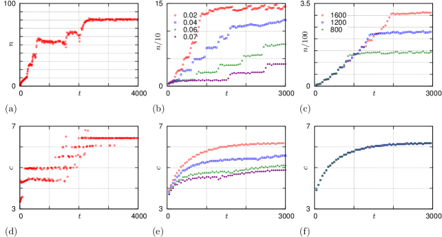
Figure 8: The dynamics of (a–c) numbers of wavelets and (e–h) velocities of the envelope waves in multi-envelop quasi-soliton regimes. (a,d) The quantities measured in a finite $L$ with periodic boundary conditions; the same simulation as shown in fig. 7. (b,e) The quantities are measured for the headmost $L=800$ interval of a wavetrain in an “infinite length” computations, for $\varepsilon=0.01$, $k_{1}=10$ and selected values of $a$ as indicated in the legend. (c,f) The quantities are measured for $\varepsilon=0.01$, $k_{1}=10$ and $a=0.02$, with different measurement length $L$ as indicated in the legend. In panel (f), the velocities measured for different $L$ are indistinguishable.

Panels (a,d) of fig. 8 analyse the dynamics of the number of wavelets and the group (envelope) velocity for the simulation shown in fig. 7. Both the wavelet number and the group velocity grow, albeit non-monotonincally, till reaching stable constant values, which corresponds to establishment of the stationary regime of three envelopes shown in fig. 7. We stress that the group velocity of the established multi-envelope soliton regime in a circle is always higher than the speed of a similar regime on the “infinite line”, which is illustrated in fig. 8(b,e): there the speed is established monotonically, and the number of envelopes constantly increases. In Tsyganov et al. (2009) we have demonstrated that in a cross-diffusion excitable system, the speed of a periodic train of waves can be faster for smaller periods. There we called this effect “negative refractoriness”, meaning, using electrophysiological terminology, that in the relative refractory phase the excitability is enhanced rather than suppressed. In the present case, we observe a similar negative refractoriness effect on the higher level of the hierarchy, for envelope quasi-solitons (groups of waves) rather than individual waves.

To conclude the analysis of the wavelet number and group speeds for multi-envelope quasi-solitons, we note that for the MEQS on an “infinite line”, as should be expected, does not depend on the length of the interval used for computations, and the number of envelope, obviously, does, see fig. 8(c,f).

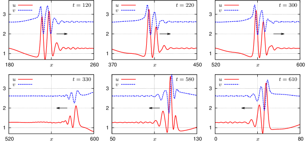
Figure 9: Quasi-soliton interaction of an envelope soliton with an impermeable boundary in LE model (2,6), $A=6.35$, $B=0.045$.

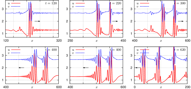
Figure 10: Formation of a multi-envelope quasi-soliton and its interaction with an impermeable boundary in LE model (2,6), with $A=6.45$, $B=0.045$.

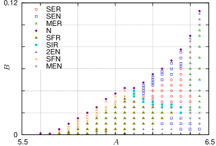
Figure 11: Parametric regions in the $(A,B)$ plane for different wave regimes in LE model (2,6),. The nomenclature of the wave regimes is the same as in fig. 2.

III.3 Lengyell-Epstein kinetics

Results of our numerical experiments with the reaction–cross-diffusion system (2) with the LE kinetics (6) are qualitatively similar to those with the FHN kinetics (5), described above. Fig. 9 illustrates the collision of an EQS with an impremeable boundary for the LE kinetics. We can see that the amplitudes of the wavelets decrease upon the collision ($t=330$) and then recover to their stationary values ($t=580$, $t=610$). Similarly, fig. 10 illustrates formation of MEQS and their interaction with the boundary for the LE kinetics. The parametric portrait in the $(A,B)$ plane is shown in fig. 11. All the qualitatively distinct regimes identified for the FHN kinetics and shown in fig. 2, have been also found for the LE kinetics and shown in fig. 11.

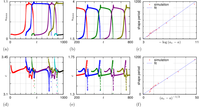
Figure 12: Dynamics of quasi-solitons in the transitional area ’SIR’ in figures 2(a) and 11. (a,b) amplitudes and (d,e) velocities of individual wavelets of quasi-solitons; (a,d) FHN model (2,5), $a=0.18$, $\varepsilon=0.006$. (b,e) LE model (2,6), $A=6.25$, $B=0.025$. (c,f) Dependence of the quasi-soliton shape change period in the FHN model as a function of parameter $a$ at fixed $\varepsilon=0.005$, and its best fits by the theoretical dependencies (10) and (11) respectively. See the last episode of Fig02 movie in the Supplementary material epa .

III.4 More exotic regimes

Finally, we consider two more regimes to complete our overview.

The “single intermediate reflecting” (SIR) regime found both in fig. 2(a) and fig. 11 is “intermediate” in the sense that it periodically changes its shape as it propagates, in which sense it is similar to the envelope quasi-soliton; however most of the time it propagates nearly as a simple quasi-soliton. Only during relatively short episodes, the wave undergoes transformation, whereby it looses a wavelet at the tail and begets one at the front, and these episodes are separated by relatively long periods when the wave retains a constant shape. The dynamics of the parameters of such a regime is shown in fig. 12(a,b,d,e). This phenomenology is reminiscent of a limit cycle born through bifurcation of a homoclinic orbit. In our present context, this would of course be an equivariant bifurcation with respect to the translations along the $x$ axis, or the bifurcation in the quotient system, i.e. the system describing the evolution of the shape of the propagating wave, as opposed to position of that wave (see Biktashev et al. (1996); Biktashev and Holden (1998); Chossat (2002); Foulkes and Biktashev (2010)). Correspondingly, the limit cycle presents itself as the periodic repetition of the shapes of the quasi-solitons, rather than periodic solutions in the usual sense. In the qualitative theory of ordinary differential equations, there are two classical examples, which predict different dependencies of the period on the bifurcation parameter. One is the bifurcation of a homoclinic loop of a saddle point Shilnikov (1962); the other is the bifurcation of a homoclinic loop of a saddle-node Shilnikov (1963), also known as SNIC (saddle-node in the invariant circle) bifurcation, SNIPER (Saddle-Node Infinite Period) bifurcation and “infinite period” bifurcation; see e.g. (Strogatz, 2000, Chapter 8.4). In the case of a homoclinic of a saddle, the expected dependency is

$$T\approx C_{1}+C_{2}\log\left(|a-a_{*}|\right),$$ (10)

where $a_{*}$ is the critical value of the bifurcation parameter $a$ and $C_{1}$ and $C_{2}$ are some constants. For the bifurcation of the homoclinic loop of a saddle-node, the asymptotic is different,

$$T\approx C_{3}|a-a_{*}|^{-1/2}$$ (11)

for some constant $C_{3}$. The fitting of the dependence of the soliton shape period on the bifurcation parameter $a$ in the FHN kinetics by (10) and (11) is shown in fig. 12, panels (c) and (f) respectively. In our case, the hypothetical limit cycles exist for $a<a_{*}$, and the best-fit bifurcation value for (10) is $a_{*}\approx 0.206477$, whereas for (11) it is $a_{*}\approx 0.206925$.

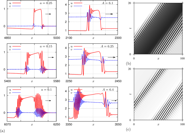
Figure 13: (a) Profiles of established wave regimes for parameters from the ‘Z’ zones in figures 2(a) and 11. Left column: FHN model (2,5) for $\varepsilon=0.001$ and $a=0.25$, $a=0.15$ and $a=0.1$ as shown by the legends. Right column: LE model (2,6) for $B=0.001$ and $A=6.1$, $A=6.25$ and $A=6.4$, as shown by the legends. (b,c) Fragment of a density plot of respectively the $u$ and $v$ variables for the FHN model with $a=0.1$.

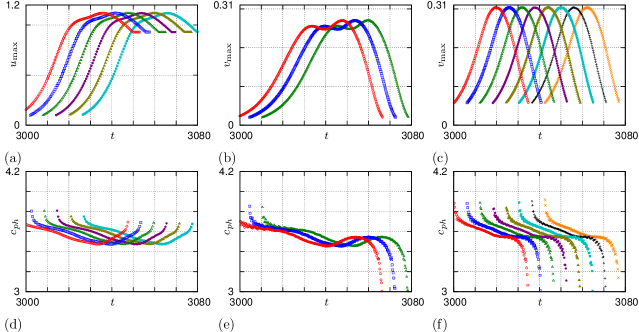
Figure 14: Dynamics of the (a–c) amplitudes and (d–f) velocities of individual wavelets, (a,d) of the $u$-variable in the front zone, (b,e) of the $v$-variable in the front zone, (c,f) of the $v$-variable in the back zone, for the FHN model (2,5) at $k_{1}=10$, $a=0.1$, $\varepsilon=0.001$, see top bottom left panel of fig. 13(a).

The other regime is “double-envelope non-reflecting” (2EN) and it has separate “envelope” trains at the front and at the back, separated by a non-oscillating plateau, see fig. 13. The corresponding dynamics of the wavelet amplitudes and their speeds is shown in fig. 14. This regime is observed for smaller values of $\varepsilon$ in the FHN kinetics (fig. 2(a)) and smaller values of $B$ in the LE kinetics (fig. 11).

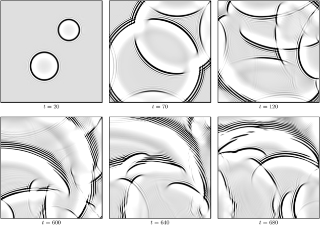
Figure 15: Selected snapshots of “wave flocks” of envelope quasi-solitons in 2D FHN model with $a=0.02$, $\varepsilon=0.01$, $k_{1}=5$, $h_{1}=h_{2}=0.3$, box size $140\times 140$. See Supplementary Material epa for a movie.

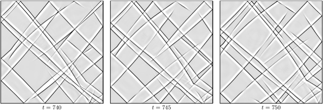
Figure 16: Selected snapshots of “wave grid” of quasi-solitons in 2D FHN model with $a=0.02$, $k_{1}=30$, $\varepsilon=0.01$, $h_{1}=h_{2}=0.1$, box size $140\times 140$. See Supplementary Material epa for a movie.

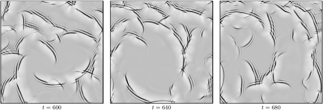
Figure 17: Selected snapshots of “wave flocks” of envelope quasi-solitons in 2D LE model with $A=6.4$, $B=0.04$, $h_{1}=0.3$, $h_{2}=0.3$, box size $140\times 140$. See Supplementary Material epa for a movie.

III.5 Quasi-solitons in two spatial dimensions

In Biktashev et al. (2004) we have shown that simple quasi-soliton waves in two-dimensional excitable systems with cross-diffusion can penetrate or break on collision. Whether the wavebreak occurs or not depended on curvature and thickness of the waves, and also on the angle of their collision, leading to emergence of complicated patterns. The two-dimensional extensions of the envelope and multi-envelope quasi-solitons are no simpler; we present here only a few selected examples, see figures 15–17. The wavebreaks can occur to whole wavetrains, as well as modify the number of a wavelets in a train, and the result of a collision depends on the time interval since a previous collision, so that encounters occuring in a quick succession are more likely to lead to wavebreaks. This can lead to “wave flocks”, that is, wave groups bounded not only lenthwise but also sidewise, see fig. 15 and 17. For comparison, fig. 16 shows development of a “wave grid” of two-dimensional simple quasi-solitons, i.e. the case where every wave has exactly one wavelet; another reason for a different appearance is that the waves at these parameters are more robust than those in figures 15 and 17, and are broken less often, hence the typical sidewise extent of the wave fragments is significantly longer.

IV Discussion

Solitons have attracted an enormous attention both from mathematical viewpoint and from applications, ever since their discovery. For applications, it has been always understood that the classical solitons are an idealization, and it is therefore interesting to study systems and solutions similar to solitons in different aspects and in various degrees. Zakharov and Kuznetsov Zakharov and Kuznetsov (1998), discussing optical solitons, commented (translation is ours): “Objects called solitons in nonlinear optics are not solitons in the strict sense of the word. Those are quasi-solitons, approximate solutions of the Maxwell equations, depending on four parameters. Real stationary solitons, which propagate with constant speed and without changing their form, are exact solutions of the Maxwell equations, depending on two parameters.…” We mention in passing that we are using the word “quasi-solitons” in a different sense than Zakharov and Kuznetsov (1998); however, the main message is that the completely integrable systems like nonlinear Schrödinger equation are always an idealization and in real life one is interested in broader class of equations and a broader class of solutions.

The nonlinear dissipative waves in excitable and self-oscillatory systems are traditionally considered an entirely different sort of things from the integrable systems displaying the classical solitons: the words “active media” and “autowaves” are sometimes also used to characterize this different “world”.

The excitable media with cross-diffusion that we considered in this paper are somewhat intermediate in that they present features in common to both these different “worlds”. On one hand, in a large areas of parameters, we observe reflection from boundaries and penetration through each other, although with a brief decrease, but without change in shape and amplitude in the long run. The link to dissipative waves is that in the established regimes have amplitude and speed depending on the system parameters rather than initial conditions.

In this paper, we have reviewed parametric regions and properties of a few different regimes, such as simple quasi-solitons (corresponding to classical solitons in integrable systems), envelope quasi-solitons (corresponding to envelope, or group solitons, or breathers in integrable systems). We have identified a transitional region between simple and envelope quasi-solitons, which displays features of a homoclinic bifurcation in the quotient system. We also have described a regime we called multi-envelope quasi-solitons. This regime presents a next level of hierarchy, after simple quasi-solitons (“solitary” wave, stationary solution in a co-moving frame of reference) and envelope quasi-solitons (“group” wave, periodic solution in a co-moving frame of reference), which are “groups of groups of waves” and apparently quasi-periodic solutions in a co-moving frame of reference. One naturally wonders if this is the last level in thid hierarchy or more complicated structures may be observed after a more careful consideration — however this is far beyond the framework of the present study.

We have limited our consideration, with two simple exceptions, to a purely empirical study, leaving a proper theoretical investigation for the future. The two exceptions are that we confirm that the oscillating fronts of the simple quasi-solitons and envelope quasi-solitons observed in numerical simulations are in agreement with the linearized theory, and that the periods of the quasi-solitons in the transitional zone between simple and envelope are consistent with a homoclinic bifurcation in a co-moving frame of reference. Further theoretical progress may be achievable either by studying of the quasi-soliton solutions as boundary-value problems by their numerical continuation and bifurcation analysis, or by asymptotic methods. At present we can only speculate that one possibility is the limit of many wavelets per envelope, which is inspired by observation that in this limit the shape of the wavelets is nearly sinusoidal, so some kind of averaging procedure may be appropriate in which the fast-time “wavelet” subsystem is linear and the nonlinearity only acting in the averaged slow-time “envelope” subsystem. We have already commented in Biktashev and Tsyganov (2011) that treating cross-diffusion FitzHugh-Nagumo system as a dissipative perturbation of the nonlinear Schrödinger equation does not work out. A further observation is that apparently this separation of time scales cannot be uniform, as some parts of the envelope quasi-solitons that indeed look as amplitude-modulated harmonic “AC” oscillations with a slow “DC” component, such as the head and the main body of the EQS illustrated in fig. 1(b), and the “front” and “back” oscillatory pieces of the “double-envelope” regime shown in  fig. 13, and some other parts which have only the slow component but no oscillating component, such as the tail of the EQS of fig. 1(b) and the plateau and the tail of the double-envelope wave of fig. 13. This suggests that any asymptotic description of these waves will have to deal with matched asymptotics.

The systems we consider are not conservative, and the natural question is where such systems can be found in nature. We have mentioned in the Introduction a number of applications that motivate consideration reaction-diffusion system with cross-diffusion components; a more extensive discussion of that can also be found in Vanag and Epstein (2009). Regimes resembling quasi-solitons and finite-length wavetrains phenomenologically have been observed in various places. The review Vanag and Epstein (2009) describes a number of unusual wave regimes obtained in Belousov-Zhabotinsky (BZ) type reactions in microemulsions, including e.g. “jumping waves” and “packet waves”, which share some phenomenology with the group quasi-solitons. The “packet waves” are considered in more detail in Vanag and Epstein (2002, 2004), which demonstrate, in particular, cases of quasi-solitonic behaviour of those, i.e. reflection from boundaries, see fig. 5(e) in Vanag and Epstein (2004) paper—although it is difficult to be sure if it is the same as our group quasi-solitons as too little detail are given. Those packet waves have been reproduced in a model with self-diffusion only, but with three components. Another example of complicated wave patterns which may be related to quasi-solitons is given in Manz et al. (2006), with experimental observations in a variant of BZ reaction as well as numerical simulation; again the simulations there were for a three-component reaction-diffusion system with self-diffusion only. Regarding chemical systems, we must note that the models we considered here may not be expected to be realised literally. Apart from the choice of the kinetic functions and particularly of their parameters, based more on mathematical curiosity than real chemistry, the linear cross-diffusion terms as in (2) cannot describe real chemical systems as they do not guarantee positivity of solutions for positive initial conditions, so system (2) can only be considered as an idealization of (3), with corresponding restrictions. Further, our choice of the diffusivity matrix appears to be in contradiction with physical constraints related to the Second Law of Thermodynamics, which in particular require that the eigenvalues of the diffusivity matrix are real and positive, whereas ours are complex; see e.g. (Vanag and Epstein, 2009, p. 899) for a discussion. From this viewpoint, with respect to chemical systems, our solutions may be only considered as “limit cases”, presenting regimes which possibly may be continued to parameter values that are physically realisable. On the other hand, it is well known that the aforementioned constraints apply to the actual diffusion coefficients, whereas mathematical models obtained by asymptotic reduction deal with effective diffusion coefficients, and the effective diffusion matrices may well have complex eigenvalues. A famous example is the complex Ginzburg-Landau equation (CGLE); see e.g. (Kuramoto, 1984, Appendix B). This equation for one complex field, sometimes called “order parameter”, emerges as a normal form of a supercritical Hopf bifurcation in the kinetic term of a generic reaction-diffusion system. This equation can also be written, in turn, as a two-component reaction-diffusion system, for the real and the imaginary parts of the order parameter. If the original reaction-diffusion system contains no cross-diffusion terms, but the self-diffusion terms are different, then the reduced reaction-diffusion system, corresponding to the CGLE, contains the full diffusion matrix including cross-diffusion term. Moreover, in that case the two eigenvalues of the diffusion matrix are complex. Incidentally, the two effective cross-diffusion coefficients will have signs opposite to each other, as in our Eq. (2).

Speaking of other possible analogies found in literature, in nonlinear optics there is a class of phenomena called “dissipative solitons”, which also could be related to our quasi-solitons. The literature on the topic is vast; we mention just one recent example Korobko et al. (2014); for instance, compare fig. 3 in that paper with our fig. 13(a). Notice that the most popular class of models are variations of CGLE; e.g. models considered in Korobko et al. (2014) involve effective diffusion matrices precisly of the form (2). Propagating pulses of complicated shape, resembling group quasi-solitons, have also been observed in a model of blood clotting Lobanova and Ataullakhanov (2004). It is a three-component reaction-diffusion system, and “muluti-hump” shapes are observed there for non-equal diffusion coefficients. A yet another possibility is the population dynamics with taxis of species or components onto each other, such as bacterial population waves; examples of nontrivial patterns there have been presented e.g. in Tsyganov et al. (2007, 1993). A spatially extended population dynamics model considered in Kuznetsov et al. (1994) does not present complicated waveforms but is interesting as it demonstrates emergence of cross-diffusion from a model with non-equal self-diffusion-only coefficients as a result of an asymptotic procedure. Finally we mention neural networks, where “anti-phase wave patterns”, resembling group quasi-solitons, have been observed in networks of elements described by Morris-Lecar system Dmitrichev et al. (2013). The question whether all these resemblances are superficial, or there is some deeper mathematical connection behind some of them, presents an interesting topic for further investigations.

V Acknowledgements

MAT was supported in part by RFBR grants No 13-01-00333 (Russia). VNB is grateful to A. Shilnikov and J. Sieber for bibliographic advice and inspiring discussions.

References

- Merzhanov and Rumanov (1999) A. G. Merzhanov and E. N. Rumanov, Rev. Mod. Phys. 71, 1173 (1999).
- Vanag and Epstein (2009) V. K. Vanag and I. R. Epstein, Phys. Chem. Chem. Phys. 11, 897 (2009).
- Aslanidi and Mornev (1999) O. V. Aslanidi and O. A. Mornev, Journal of Biological Physics 25, 149 (1999).
- Tsyganov et al. (2003) M. A. Tsyganov, J. Brindley, A. V. Holden, and V. N. Biktashev, Phys. Rev. Lett. 91, 218102 (2003).
- Biktashev and Tsyganov (2005) V. N. Biktashev and M. A. Tsyganov, Proc. Roy. Soc. Lond. A 461, 3711 (2005).
- Biktashev and Tsyganov (2011) V. N. Biktashev and M. A. Tsyganov, Phys. Rev. Lett. 107, 134101 (2011).
- Malomed (2005) B. Malomed, in Encyclopedia of Nonlinear Science, edited by A. Scott (Routledge, New York and London, 2005), pp. 639–642.
- Cartwright et al. (1997) J. H. E. Cartwright, E. Hernandez-Garcia, and O. Piro, Phys. Rev. Lett. 79, 527 (1997).
- Chung and Peacock-López (2007) J. M. Chung and E. Peacock-López, Phys. Lett. A 371, 41 (2007).
- Tsyganov et al. (2007) M. A. Tsyganov, V. N. Biktashev, J. Brindley, A. V. Holden, and G. R. Ivanitsky, Physics-Uspekhi 50, 275 (2007).
- Murray (2003) J. D. Murray, Mathematical Biology II: Spatial Modes and Biomedical Applications (Springer, New York etc, 2003).
- Tsyganov et al. (2004) M. A. Tsyganov, J. Brindley, A. V. Holden, and V. N. Biktashev, Physica D 197, 18 (2004).
- Lengyel and Epstein (1991) I. Lengyel and I. R. Epstein, Science 251, 650 (1991).
- (14) See EPAPS Document No. [number will be inserted by publisher] for movies illustrating some of the figures. For more information on EPAPS, see http://www.aip.org/pubservs/epaps.html.
- Tsyganov et al. (2009) M. A. Tsyganov, V. N. Biktashev, and G. R. Ivanitsky, Biofizika 54, 704 (2009).
- Biktashev et al. (1996) V. N. Biktashev, A. V. Holden, and E. V. Nikolaev, Int. J. of Bifurcation and Chaos 6, 2433 (1996).
- Biktashev and Holden (1998) V. N. Biktashev and A. V. Holden, Physica D 116, 342 (1998).
- Chossat (2002) P. Chossat, Acta Appplicandae Mathematicae 70, 71 (2002).
- Foulkes and Biktashev (2010) A. J. Foulkes and V. N. Biktashev, Phys. Rev. E 81, 046702 (2010).
- Shilnikov (1962) L. Shilnikov, Soviet Math. Dokl. 3, 394 (1962), in Russian.
- Shilnikov (1963) L. Shilnikov, Mat. Sbornik 61, 443 (1963), in Russian.
- Strogatz (2000) S. H. Strogatz, Nonlinear dynamics and chaos : with applications to physics, biology, chemistry, and engineering (Westview Press, Cambridge, Mass., 2000).
- Biktashev et al. (2004) V. N. Biktashev, J. Brindley, A. V. Holden, and M. A. Tsyganov, Chaos 14, 988 (2004).
- Zakharov and Kuznetsov (1998) V. E. Zakharov and E. A. Kuznetsov, J. Exp. Theor. Phys. 113, 1892 (1998).
- Vanag and Epstein (2002) V. K. Vanag and I. R. Epstein, Phys. Rev. Lett. 88, 088303 (2002).
- Vanag and Epstein (2004) V. K. Vanag and I. R. Epstein, J. Chem. Phys. 121, 890 (2004).
- Manz et al. (2006) N. Manz, B. T. Ginn, and O. Steinbock, Phys. Rev. E 73, 066218 (2006).
- Kuramoto (1984) Y. Kuramoto, Chemical Oscillations, Waves and Turbulence (Springer-Verlag, Berlin Heidelberg New York Tokyo, 1984).
- Korobko et al. (2014) D. A. Korobko, R. Gumenyuk, I. O. Zolotovskii, and O. G. Okhotnikov, Opt. Fiber Technol. http://dx.doi.org/10.1016/j.yofte.2014.08.011 (2014).
- Lobanova and Ataullakhanov (2004) E. S. Lobanova and F. I. Ataullakhanov, 93, 098303 (2004).
- Tsyganov et al. (1993) M. A. Tsyganov, I. B. Kresteva, A. B. Medvinsky, and G. R. Ivanitsky, Doklady 333, 532 (1993).
- Kuznetsov et al. (1994) Y. A. Kuznetsov, M. Antonovsky, V. N. Biktashev, and E. A. Aponina, J. Math. Biol. 32, 219 (1994).
- Dmitrichev et al. (2013) A. S. Dmitrichev, V. I. Nekorkin, R. Behdad, S. Binczak, and J. M. Bilbault, Eur. Phys. J. Special Topics pp. 2633–2646 (2013).