On the nature of heat in strongly coupled open quantum systems

Abstract

We study heat transfers in a single level quantum dot strongly coupled to fermionic reservoirs and subjected to a time-dependent protocol modulating the dot energy as well as the dot-reservoir coupling strength. The dynamics is described using nonequilibrium Greens functions (NEGFs) evaluated to first order beyond quasi-static driving. We show that any heat definition expressed as an energy change in the reservoir energy plus any fraction of the system-reservoir interaction is not an exact differential when evaluated along reversible isothermal transformations, except when that fraction is zero. However, even in that latter case the reversible heat divided by temperature, namely the entropy, does not satisfy the third law of thermodynamics and diverges in the low temperature limit. Our results cast doubts on the possibility to define a thermodynamically consistent notion of heat expressed as the expectation value of some Hamiltonian terms.

The nature of heat is one of the most fundamental questions which has been driving research in thermodynamics since its origins. Nowadays, establishing a thermodynamically consistent notion of heat for open quantum system is of crucial importance for mesoscopic physics and for the study of energy conversion in small devices. This issue has direct implications on defining meaningful notions of efficiency in thermoelectricity or photoelectricity for instance.

For systems weakly interacting with their reservoirs the situation is rather clear Spohn and Lebowitz (2007); Breuer and Petruccione (2002); Esposito (2012); Kosloff (2013); Gelbwaser-Klimovsky et al. (2015); Bulnes Cuetara et al. (2015); Esposito et al. (2009a). The heat flux is defined as minus the energy change in the reservoir and can be directly related to the system energy changes since the system-reservoir coupling energy is negligible. This definition has been extensively used to study the performance of a broad range of nano-devices (see e.g. Esposito et al. (2009b); Rutten et al. (2009); Esposito et al. (2010a); Esposito et al. (2012); Sanchez et al. (2010); Sánchez and Büttiker (2011); Entin-Wohlman and Aharony (2012); Entin-Wohlman et al. (2010); Benenti et al. (2013); Roßnagel et al. (2014); Correa et al. (2013); Uzdin et al. (2015); Esposito et al. (2015a)).

The situation is also clear in the strong coupling regime, as long as the system operates in a steady state Whitney (2013); Gaspard (2015); Topp et al. (2015) (see also e.g. Dhar et al. (2012); Martinez and Paz (2013)). Indeed attributing the coupling energy to the system or to the reservoirs is equivalent in this case since net changes in the coupling energy are zero. The first law reduces to Kirchhoff’s law for heat fluxes crossing the system and the second law reduces to the non-negativity of $-\sum_{\nu}\dot{Q}_{\nu}/T_{\nu}\geq 0$ where $\dot{Q}_{\nu}$ is the heat entering the system from reservoir $\nu$ and $T_{\nu}$ is the temperature of that reservoir. This result can easily be shown using scattering theory or nonequilibrium Green’s functions (NEGF) approaches. Many performance studies have thus considered steady state setups (see e.g. Humphrey et al. (2002); Humphrey and Linke (2005); Schaller et al. (2013); Krause et al. (2015); Whitney (2014); Brandner et al. (2013); Brandner and Seifer (2013)).

However, the situation is very different when considering setups where the system is driven by a time-dependent processe since in this case the changes in the coupling energy must be accounted for. Despite the fact that such setups are indispensable to consider reversible transformations which play a central role in thermodynamics, few studies have considered them because the dynamics typically becomes difficulty to solve. We recently proposed a consistent nonequilibrium thermodynamics formulation for noninteracting quantum systems strongly coupled to their reservoirs and driven by a slowly changing external field Esposito et al. (2015b). Within the framework of NEGF we calculated transport characteristics to first order beyond quasi-static limit. This formulation has the particularity that not only heat but all the other thermodynamic quantities such as work, system energy and entropy have no simple expression in terms of quantum expectations values of operators. In this letter, we use the same framework of NEGF to show that any attempt to define heat in term of quantum expectations values of operators leads to thermodynamic inconsistencies.

The typical Hamiltonian of an open quantum system $S$ coupled to multiple reservoirs $\nu$ at temperatures $T_{\nu}$ and chemical potentials $\mu_{\nu}$ is

$$\hat{H}(t)=\hat{H}_{S}(t)+\sum_{\nu}\left(\hat{H}_{\nu}+\hat{V}_{\nu}(t)\right),$$ (1)

where $\hat{H}_{S}$ ($\hat{H}_{\nu}$) denotes the system (reservoir $\nu$) Hamiltonian and $\hat{V}_{\nu}$ is the system-reservoir interaction.

We start by introducing the class of all possible heat definitions expressed as the change in the quantum expectation value of the reservoir Hamiltonian plus a fraction $0\leq\alpha\leq 1$ of the the system-reservoir coupling energy (we set $\hbar=e=k_{B}=1$ throughout the paper)

$$\dot{Q}_{\nu,\alpha}=J_{\nu,\alpha}-\mu_{\nu}I_{\nu},$$ (2)

where the matter and heat currents entering the system from reservoir $\nu$ are given by

$$I_{\nu}= -{\rm Tr}\{\hat{N}_{\nu}\,d_{t}\hat{\rho}\}=-d_{t}\langle\hat{N}_{\nu}\rangle$$ (3)

$$J_{\nu,\alpha}= -{\rm Tr}\{\big{(}\hat{H}_{\nu}+\alpha\hat{V}_{\nu}\big{)}d_{t}\hat{\rho}\},$$ (4)

and $\hat{\rho}(t)$ is the density matrix of the total system. The heat flux definition most commonly used in the literature corresponds to the choice $\alpha=0$ and can be expressed in terms of the rate of change in the number operator $\hat{N}_{\nu}$ and in the Hamiltonian $\hat{H}_{\nu}$ of the reservoir $\nu$, since $J_{\nu,0}=-d_{t}\langle\hat{H}_{\nu}\rangle$ Mahan (2010); Galperin et al. (2007); Wu and Segal (2009); Segal (2013); Esposito et al. (2010b); Pucci et al. (2013); Martinez and Paz (2013). The choice $\alpha=1$ was considered for instance in Ref. Allahverdyan and Nieuwenhuizen (2001) and the choice $\alpha=1/2$ in Ref. Ludovico et al. (2014).

The specific model that we will consider consists of an externally driven level $\varepsilon(t)$ bi-linearly coupled to a single Fermionic reservoir $R$ at equilibrium. Its Hamiltonian is given by (1), where the level, the reservoir and their coupling respectively read

$$\hat{H}_{S}(t)=\varepsilon(t)\hat{d}^{\dagger}\hat{d}\ \ ,\ \ \hat{H}_{R}=\sum_{k}\varepsilon_{k}c_{k}^{\dagger}\hat{c}_{k}$$ (5)

$$\hat{V}(t)=\sum_{k}\left(V_{k}(t)\hat{d}^{\dagger}\hat{c}_{k}+\mbox{H.c.}\right).$$ (6)

Here $\hat{d}^{\dagger}$ ($\hat{d}$) and $\hat{c}_{k}^{\dagger}$ ($\hat{c}_{k}$) create (annihilate) an electron in the level of the system and in state $k$ of the reservoir, respectively. $\varepsilon_{k}$ is the energy of the latter. We emphasize that the external driving can modify the position of the level, $\varepsilon(t)$, as well as the strength of the system-reservoir coupling, $V_{k}(t)$. Following Ref. Jauho et al. (1994), we assume that this latter is of the form

$$V_{k}(t)=u(t)\,V_{k}\qquad u(t)\in\mathbb{R}.$$ (7)

For the simulations presented in this letter we will consider the driving protocols

$$\varepsilon(t)= \varepsilon_{0}+\frac{\Delta_{\varepsilon}}{2}\bigg{(}1-\cos\omega_{0}t\bigg{)}$$ (8)

$$u^{2}(t)= 1+\frac{\Delta_{\Gamma}}{2\Gamma_{0}}\bigg{(}1-\cos\omega_{0}t\bigg{)}.$$ (9)

The explicit expression of the heat flux (2) in terms of NEGF can be found in Eqs. (S7)-(S10) of the supplementary material Esposito et al. (2015c). In general a NEGF depends on two times, $t_{1}$ and $t_{2}$, but only depends on their difference $\tau=t_{1}-t_{2}$ at steady state. If the driving acting on the system is slow compared to the system relaxation timescale, after a Fourier transform in $\tau\to E$, one can make use of the slow time-dependence of the resulting NEGF in $t=(t_{1}+t_{2})/2$ to evaluate its equation of motion. This procedure is known as the gradient expansion and is detailed in the supplementary material Esposito et al. (2015c). When using it to evaluate the heat flux for our model (5)-(7), we obtain to the lowest order corresponding to the quasi-static limit

$$\begin{split}&\dot{Q}_{\alpha}^{(1)}=\frac{d}{dt}\bigg{(}\int\frac{dE}{2\pi}f\,A^{(0)}\big{[}(E-\mu)+(1-2\alpha)(E-\varepsilon)\big{]}\bigg{)}\\ &-\int\frac{dE}{2\pi}f\bigg{(}A^{(0)}\,d_{t}{\varepsilon}+(1-\alpha)\bigg{[}\mbox{Re}\,G^{r(0)}\,\partial_{t}{\Gamma}+A^{(0)}\,\partial_{t}\Lambda\bigg{]}\bigg{)},\end{split}$$ (10)

where $f(E)=[e^{(E-\mu)/T}+1]^{-1}$ is the Fermi-Dirac distribution in the reservoir, the zero order retarded Green function is given by

$$G^{r(0)}(t,E)= \left[E-\varepsilon(t)-\Lambda(t,E)+i\Gamma(t,E)/2\right]^{-1}$$ (11)

and $A^{(0)}(t,E)=-2\,\mbox{Im}\,G^{r(0)}(t,E)$ is the system spectral function. The Lamb shift and broadening caused by coupling to the reservoir are taken asWingreen and Meir (1994); Mahan (2010)

$$\Lambda(t,E)= u^{2}(t)\,\Gamma_{0}\,\frac{1}{2}\frac{(E-E_{B})W_{B}}{(E-E_{B})^{2}+W_{B}^{2}}$$ (12)

$$\Gamma(t,E)= u^{2}(t)\,\Gamma_{0}\,\frac{W_{B}^{2}}{(E-E_{B})^{2}+W_{B}^{2}},$$ (13)

where $E_{B}$ and $W_{B}$ are the center and width of the band, respectively. To our knowledge (LABEL:QQS) is the first explicit expression for a quasi-static heat of the kind (2). Two major results ensue.

A central requirement in thermodynamics is that the reversible heat change is an exact differential. This implies that mixed derivatives of the heat rate with respect to the driving parameters $\varepsilon(t)$ and $u(t)$ should be equal to each other

$$\frac{\partial^{2}Q^{(1)}_{\alpha}}{\partial\varepsilon\,\partial u}=\frac{\partial^{2}Q^{(1)}_{\alpha}}{\partial u\,\partial\varepsilon}.$$ (14)

Our first important result is that this property is only satisfied for $\alpha=0$. For any other choice of $\alpha$, the reversible heat is not an exact differential and thus cannot be considered as a thermodynamically consistent definition. This result can be explicitly seen in Fig.1 where two different reversible driving protocols connecting the same initial and final point give rise to different reversible heat except for $\alpha=0$.

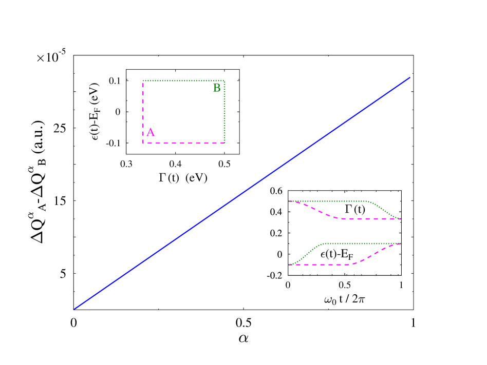
Figure 1: (Color online) Difference between the quasi-static heat produced along two different driving protocols denoted by A and B and corresponding to (8) and (9) with parameters $T=10$ K, $\varepsilon_{0}=-0.1$ eV, $\Delta_{\varepsilon}=0.2$ eV, $\Delta_{\Gamma}=-1/6$ eV, $\Gamma_{0}=0.5$ eV, $\omega_{0}=10^{13}$ s^-1. The band parameters are $E_{B}=0$ and $W_{B}=5$ eV and the Fermi energy is $E_{F}=0$. The two protocols are shown in the left top inset and the time dependence of the level position and coupling strength corresponding to the protocols are given in the bottom right inset.

Our second important result is that since the equilibrium entropy is the state function whose differential is the reversible heat divided by temperature $d_{t}S^{eq}=\dot{Q}_{0}^{(1)}/T$, by integrating the reversible heat rate (LABEL:QQS), we are able to find the equilibrium entropy up to a constant (see Esposito et al. (2015c))

$$S^{eq}= \int\frac{dE}{2\pi}A\big{(}-f\ln f-[1-f]\ln[1-f]\big{)}$$

$$+\int\frac{dE}{2\pi}Af\frac{(E-\varepsilon)}{T}$$ (15)

$$+\int\frac{dE}{2\pi}A\ln[1-f]\big{(}\partial_{E}\Lambda+\frac{E-\varepsilon-\Lambda}{\Gamma}\partial_{E}\Gamma\big{)}.$$

The first contribution has the appealing form of an energy resolved equilibrium entropy. The second one is exactly half of the equilibrium expectation value of the coupling energy divided by temperature, namely $\langle\hat{V}_{\nu}(t)\rangle^{eq}/(2T)$. The third one is due to the energy resolution of the Lamb shift and broadening and thus vanishes in the wide-band limit when $\Lambda\to 0$ and $\Gamma$ does not depend on energy. In the low temperature limit $T\to 0$, the first terms goes to zero as expected by the third law of thermodynamics, but the other two terms diverge, casting doubts on the thermodynamic relevance of the heat definition $\dot{Q}_{0}$. The only way to avoid the divergence is to send the coupling strength to zero before taking the low temperature limit. Indeed, in this case the first term becomes the weak coupling Shannon entropy and the last two vanish. While one may have expected that the finite coupling can create a finite entropy in the system at low temperature, justifying a divergent entropy is more difficult and seems pathological. In Figure 2 we compare the behavior of the entropy change obtained from the reversible heat $Q_{0}^{(1)}$ given by (LABEL:QQS) and the reversible heat ${\cal Q}$ that we recently proposed in Ref. Esposito et al. (2015b). The low temperature divergence is clearly seen in the first case but not in the second one, as proved in Esposito et al. (2015b).

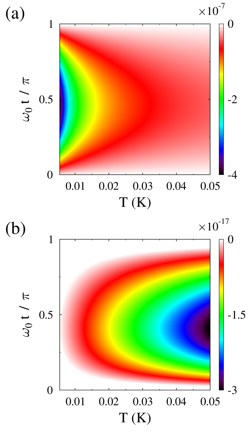
Figure 2: (Color online) Entropy change ($J/K\,s$) given by (a) Eq.(62) and (b) Eq.(14) in Ref. Esposito et al. (2015b), as a function of temperature and the time along half of the period performed by the driving (8) and (9) with $\varepsilon_{0}=\Delta_{\varepsilon}=0$, $\Delta_{\Gamma}=1/6$ eV, $\Gamma_{0}=0.5$ eV, $\omega_{0}=10^{14}$ s^-1. The other parameters are the same as in Fig. 1.

We now consider the heat generated along the cycle of a periodic driving when the system reached a stationary regime (i.e when initial transients are gone). Since the quasi-static heat vanishes along a cycle, on must calculate its second order contribution. Its general expression is derived in the supplementary material Esposito et al. (2015c). When integrated over a cycle of duration $\tau$ for $\alpha=0$, the resulting heat reads $Q_{0}^{(2)}=$

$$\int_{0}^{\tau}dt\int\frac{dE}{2\pi}\partial_{E}f\frac{\left[A^{(0)}\right]^{2}}{2}\bigg{(}d_{t}\varepsilon+\partial_{t}\Lambda+\partial_{t}\Gamma\frac{E-\varepsilon-\Lambda}{\Gamma}\bigg{)}^{2}.$$ (16)

Since $\partial_{E}f$ is always negative, this heat is always negative in agreement with the second law of thermodynamics.

We finally comment on the heat definition $Q_{1/2}$ proposed in Ref. Ludovico et al. (2014) when considering a strongly coupled ac-driven resonant level coupled to a single reservoir treated by scattering and Floquet theories. The couplings to the reservoirs were assumed time-independent ($u$ constant) and the wide band approximation was used. We show in the supplementary material that in this limit our treatment reproduces the expression for the heat $Q_{1/2}$ found in Ref. Ludovico et al. (2014). By integrating its quasi-static form, since $T\,d_{t}S^{eq}_{1/2}=\dot{Q}_{1/2}^{(1)}$, we further show that its corresponding equilibrium entropy is given by

$$S^{eq}_{1/2}=\int\frac{dE}{2\pi}A\big{(}-f\ln f-[1-f]\ln[1-f]\big{)}.$$ (17)

This is the first contribution to the entropy found in (62). The second contribution dropped due to the choice $\alpha=1/2$ and the third due to the wide-band approximation. Since no driving in the coupling was considered, the reversible heat $Q_{1/2}^{(1)}$ is also a state function. We thus confirm that under the assumptions made in Ludovico et al. (2014) (wide band approximation and no driving in the coupling) the heat definition $\dot{Q}_{1/2}$ can be considered as very appealing. However, we proved that this definition fails when these assumptions are released.

We contributed to the fundamental question of the nature of heat in open quantum system strongly interacting with a reservoir and driven by a time-dependent force in the system and in the system-reservoir energy, within the framework of NEGF. Our central finding is that any heat definition expressed as the change in the quantum expectation value of the reservoir energy plus any fraction $\alpha$ of the coupling energy displays thermodynamic inconsistencies. Any $\alpha$ different from zero leads to a quasi-static heat which is not a state function. The choice $\alpha=0$ is more appealing (the quasi-static heat is a state function and the second law is satisfied for our model) but leads to an entropy which diverges in the low temperature limit. Our considerations were made possible by using the gradient expansion of NEGF which provides to our knowledge the first explicit quasi-static expression for the various heat definitions that we considered. This only assumption used in this approach is that the reservoir Greens functions are always thermal. Our conclusion reinforces our proposal in Ref. Esposito et al. (2015b) to abandon heat definitions (and other thermodynamic quantities) expressed as quantum expectation values of operators in order to derive a consistent thermodynamics within the framework of NEGF for open quantum system beyond the weak coupling limit.

Appendix A Particle and energy fluxes

We consider the standard definition for the particle and energy fluxes at the interface with reservoir $\nu$, Eqs. (3) and (4), respectively. In terms of Green functions, these definitions yield Jauho et al. (1994); Galperin et al. (2007)

$$I_{\nu}(t)= 2\,\mbox{Re}\,\mbox{Tr}\int dt_{1}\big{\{}G^{<}(t,t_{1})\,\Sigma_{\nu}^{a}(t_{1},t)$$ (18)

$$\qquad\qquad\quad+G^{r}(t,t_{1})\,\Sigma_{\nu}^{<}(t_{1},t)\big{\}}$$

$$J_{\nu,\alpha}(t)= (\alpha-1)\,\partial_{t}\langle\hat{V}_{\nu}(t)\rangle-\alpha\,d_{t}\langle\hat{V}_{\nu}(t)\rangle$$

$$+ 2\,\mbox{Im}\,\mbox{Tr}\int dt_{1}\big{\{}G^{<}(t,t_{1})\,\partial_{t}\Sigma_{\nu}^{a}(t_{1},t)$$ (19)

$$\qquad\qquad\quad+G^{r}(t,t_{1})\,\partial_{t}\Sigma_{\nu}^{<}(t_{1},t)\big{\}},$$

where

$$\langle\hat{V}_{\nu}(t)\rangle= 2\,\mbox{Im}\,\mbox{Tr}\int dt_{1}\big{\{}G^{<}(t,t_{1})\,\Sigma_{\nu}^{a}(t_{1},t)$$ (20)

$$\qquad\qquad\quad+G^{r}(t,t_{1})\,\Sigma_{\nu}^{<}(t_{1},t)\big{\}}.$$

The partial derivatives in the first and third terms in the right side of Eq.(A) indicate a time derivative of the system-reservoir coupling only in the external driving. $\mbox{Tr}\{\ldots\}$ denotes a trace over the system subspace. $G^{<}=G^{-+}$ and $G^{r}=G^{--}-G^{-+}$ are matrices in the system subspace and are the lesser and retarded projections of the single-particle Green function

$$G_{mm^{\prime}}(\tau,\tau^{\prime})=-i\left\langle T_{c}\,\hat{d}_{m}(\tau)\,\hat{d}_{m^{\prime}}^{\dagger}(\tau^{\prime})\right\rangle,$$ (21)

where $T_{c}$ denotes the contour ordering operator, $\tau$ and $\tau^{\prime}$ are the contour variables, and the contour branches are labeled as time ordered, $s={}-{}$, and anti-time ordered, $s={}+{}$. $\Sigma_{\nu}^{<}=\Sigma_{\nu}^{-+}$ and $\Sigma_{\nu}^{a}=\Sigma_{\nu}^{-+}-\Sigma_{\nu}^{++}$ are also matrices in the system space and are the lesser and advanced projections of the self-energy due to the coupling to reservoir $\nu$

$$\left[\Sigma_{\nu}(\tau,\tau^{\prime})\right]_{mm^{\prime}}=\sum_{k\in\nu}V_{mk}(t)\,g_{k}(\tau,\tau^{\prime})\,V_{km^{\prime}}(t^{\prime}),$$ (22)

where

$$g_{k}(\tau,\tau^{\prime})\equiv-i\langle T_{c}\,\hat{c}_{k}(\tau)\,\hat{c}_{k}^{\dagger}(\tau^{\prime})\rangle$$ (23)

is the equilibrium Green function for the free electrons in the reservoir $\nu$. The equations of motion for the projection $s_{1}s_{2}$ of the GF (21) are given by

$$\left(i\frac{\overset{\rightarrow}{\partial}}{\partial t_{1}}\sigma^{z}_{s_{1}s_{2}}-H_{S}(t_{1})\right)G^{s_{1}s_{2}}(t_{1},t_{2})=$$ (24)

$$\quad\sigma^{z}_{s_{1}s_{2}}\delta(t_{1}-t_{2})-\sum_{s_{3}}\int dt_{3}\,\Sigma^{s_{1}s_{3}}(t_{1},t_{3})\,s_{3}\,G^{s_{3}s_{2}}(t_{3},t_{2})$$

$$G^{s_{1}s_{2}}(t_{1},t_{2})\left(-i\frac{\overset{\leftarrow}{\partial}}{\partial t_{2}}\sigma^{z}_{s_{1}s_{2}}-H_{S}(t_{2})\right)=$$ (25)

$$\quad\sigma^{z}_{s_{1}s_{2}}\delta(t_{1}-t_{2})-\sum_{s_{3}}\int dt_{3}\,G^{s_{1}s_{3}}(t_{1},t_{3})\,s_{3}\,\Sigma^{s_{3}s_{2}}(t_{3},t_{2}),$$

where $\mathbf{\sigma}^{z}$ is the Pauli matrix, and $\Sigma^{s_{1}s_{2}}(t_{1},t_{2})$ is the total self-energy, i.e. the self-energy due to the system-reservoirs couplings and the intra-system interactions.

Appendix B Gradient expansion

Green functions and self-energies are two-time functions, $F(t_{1},t_{2})$. Introducing via a change of variable the classical timescale, $t=(t_{1}+t_{2})/2$, and the quantum timescale, $s=t_{1}-t_{2}$, and performing a Fourier transform in the quantum time leads to the time-dependent energy resolved function $F(t,E)=\int dse^{iEs}F(t,s)$, which is the Wigner transform of $F(t,s)$. Naturally

$$F(t_{1},t_{2})=F(t,s)=\int\frac{dE}{2\pi}\,e^{-iEs}F(t,E).$$ (26)

Below, we will consider partial derivatives of the form $\partial_{t_{2}}F(t_{1},t_{2})$ (see Eq. (A)). Their Wigner transforms read $[\partial_{t}/2+iE]F(t,E)$. We will also consider integral expression such as

$$F(t_{1},t_{2})=\int dt_{3}\,F_{1}(t_{1},t_{3})\,F_{2}(t_{3},t_{2}),$$ (27)

whose Wigner transform reads Haug and Jauho (2008)

$$F(t,E)=F_{1}(t,E)\,\hat{\mathcal{G}}(t,E)\,F_{2}(t,E),$$ (28)

where

$$\hat{\mathcal{G}}(t,E)=\mbox{exp}\left(\frac{1}{2i}\left[\overset{\leftarrow}{\partial}_{t}\,\overset{\rightarrow}{\partial}_{E}-\overset{\leftarrow}{\partial}_{E}\,\overset{\rightarrow}{\partial}_{t}\right]\right)$$ (29)

is the gradient operator. At steady state the dependence on $t$ vanishes and only the energy resolution $E$ survives. This means that when the driving is slow relative to the characteristic relaxation timescales of the system, we can expand (29) in Taylor series and truncate the series to the suited level. Traditionally the gradient expansion goes to the first order, but we will need the second order below

$$F(t,E)\approx F_{1}(t,E)\,F_{2}(t,E)$$ (30)

$$\qquad+\frac{i}{2}\left\{F_{1}(t,E);F_{2}(t,E)\right\}-\frac{1}{8}\left[F_{1}(t,E);F_{2}(t,E)\right],$$

where

$$\left\{F_{1}(t,E);F_{2}(t,E)\right\}=$$ (31)

$$\quad\partial_{E}F_{1}(t,E)\,\partial_{t}F_{2}(t,E)-\partial_{t}F_{1}(t,E)\,\partial_{E}F_{2}(t,E)$$

$$\left[F_{1}(t,E);F_{2}(t,E)\right]=\partial^{2}_{E}F_{1}(t,E)\,\partial^{2}_{t}F_{2}(t,E)$$ (32)

$$\quad+\partial^{2}_{t}F_{1}(t,E)\,\partial^{2}_{E}F_{2}(t,E)-\partial^{2}_{tE}F_{1}(t,E)\,\partial^{2}_{tE}F_{2}(t,E).$$

Below we will also need to consider the dependence of the full self-energy $\Sigma(t_{1},t_{2})$ on the system-reservoir coupling $u(t)$. Since

$$\Sigma(t_{1},t_{2})=u(t_{1})\,S(t_{1},t_{2})\,u(t_{2}),$$ (33)

it is easy to show that up to second order gradient expansion, the functions $\Sigma$ and $S$ are related by

$$\Sigma(t,E)\approx u^{2}(t)\,S(t,E)$$ (34)

$$- \frac{1}{4}\left(\partial^{2}_{t}u(t)-[\partial_{t}u(t)]^{2}\right)\partial_{E}^{2}S(t,E).$$

Similarly their time derivatives are related by

$$\partial_{t}\Sigma(t,E)\approx u^{2}(t)\,\partial_{t}S(t,E)+u(t)\,\partial_{t}u(t)\,S(t,E).$$ (35)

Appendix C Slow driving of a single level coupled to a reservoir

We now restrict our consideration to a single level, Eqs. (5)-(7). The position of the level $\varepsilon(t)$ as well as its coupling to the reservoir $u(t)$ are driven by a slowly changing external field, Eqs. (8)-(9).

After gradient expansion,

$$G^{r}(t_{1},t_{2})\to G^{r}(t,E)$$ (36)

$$G^{<}(t_{1},t_{2})\to G^{<}(t,E)=i\,A(t,E)\,\phi(t,E),$$ (37)

where the system spectral function is given by

$$A(t,E)\equiv-2\,\mbox{Im}\,G^{r}(t,E)$$ (38)

and $\phi(t,E)$ is the non-equilibrium population of the level. Also

$$\Sigma^{r}(t_{1},t_{2})\to\Sigma^{r}(t,E)=\Lambda(t,E)-i\Gamma(t,E)/2$$ (39)

$$\Sigma^{<}(t_{1},t_{2})\to\Sigma^{<}(t,E)=i\,\Gamma(t,E)\,f(E),$$ (40)

where $\Lambda$ and $\Gamma$ are the Lamb shift and the broadening caused by the coupling to the reservoir and $f(E)$ is the Fermi-Dirac thermal distribution.

We now apply the second order gradient expansion (30) to expressions for the fluxes, Eqs. (18) and (A). This leads to

$$I(t)=\int\frac{dE}{2\pi}\,I(t,E)=\frac{d}{dt}\int\frac{dE}{2\pi}A(t,E)\,\phi(t,E)$$ (41)

$$J_{\alpha}(t)=(\alpha-1)\,\partial_{t}\langle\hat{V}(t)\rangle+\bigg{(}\frac{1}{2}-\alpha\bigg{)}\,d_{t}\langle\hat{V}(t)\rangle$$ (42)

$$\hskip 34.14322pt+\int\frac{dE}{2\pi}\,E\,I(t,E),$$

where

$$I(t,E)=\left\{E-\varepsilon(t);A\phi\right\}$$ (43)

$$\langle\hat{V}(t)\rangle=2\int\frac{dE}{2\pi}\big{(}A\phi\,\Lambda+\mbox{Re}\,G^{r}\,\Gamma f\big{)}$$ (44)

$$\hskip 39.83368pt+\frac{1}{2}\int\frac{dE}{2\pi}\big{(}\left\{\Gamma;A\phi\right\}-\left\{\Gamma\phi;A\right\}\big{)}$$

$$\partial_{t}\langle\hat{V}(t)\rangle=\int\frac{dE}{2\pi}\big{(}A\phi\,\partial_{t}\Lambda+\mbox{Re}\,G^{r}\,\partial_{t}\Gamma\,\phi\big{)}$$ (45)

$$\hskip 45.52458pt+\frac{1}{4}\int\frac{dE}{2\pi}\big{(}\left\{\partial_{t}\Gamma;A\phi\right\}-\left\{\partial_{t}\Gamma\,\phi;A\right\}\big{)}.$$

Note that evaluation of expressions (41) and (42) up to second order in gradient expansion requires the knowledge of the $G^{r}$, $A$, and $\phi$ only up to first order (see Eqs. (49)-(53) below). Note also that in the spirit of the Botermans and Malfliet (BM) approximation Botermans and Malfliet (1990), we substituted $f(E)$ by $\phi(t,E)$ in all the expressions involving derivatives of the lesser projection of the self-energy.

The retarded projection of the Green function $G^{r}(t,E)$, the spectral function $A(t,E)$ and the non-equilibrium distribution $\phi(t,E)$ can be expanded as

$$G^{r}(t,E)=G^{r(0)}(t,E)+G^{r(1)}(t,E)+G^{r(2)}(t,E)+\ldots$$ (46)

$$A(t,E)=A^{(0)}(t,E)+A^{(1)}(t,E)+A^{(2)}(t,E)+\ldots$$ (47)

$$\phi(t,E)=\phi^{(0)}(t,E)+\phi^{(1)}(t,E)+\phi^{(2)}(t,E)+\ldots,$$ (48)

where the orders coincide with the orders of the gradient expansion. Inserting this expansion in the gradient expansion expression for the Green function equations-of-motion (24) and (25), and identifying terms order by order, one finds that Ivanov et al. (2000); Kita (2010),

$$G^{r(0)}(t,E)=\left[E-\varepsilon(t)-\Sigma^{r}(t,E)\right]^{-1}$$ (49)

$$A^{(0)}(t,E)=\frac{\Gamma(t,E)}{\left(E-\varepsilon(t)-\Lambda(t,E)\right)^{2}+\left(\Gamma(t,E)/2\right)^{2}}$$ (50)

$$\phi^{(0)}(t,E)=f(E)$$ (51)

and

$$G^{r(1)}(t,E)=A^{(1)}(t,E)=0$$ (52)

$$\phi^{(1)}=-d_{E}f\,\frac{A^{(0)}}{2}\bigg{(}d_{t}\varepsilon+\partial_{t}\Lambda+\partial_{t}\Gamma\,\frac{E-\varepsilon-\Lambda}{\Gamma}\bigg{)}.$$ (53)

C.1 Quasi-static driving

The reversible transformation in the system is performed by a quasi-static driving, which corresponds to expanding the fluxes to first order in Eqs.  (41) and (42). To do so we only need the zero order correction of the retarded Green function $G^{r\,(0)}(t,E)$, its corresponding $A^{(0)}(t,E)$, and of the population $\phi^{(0)}(t,E)$. We find

$$I^{(1)}(t)=\int\frac{dE}{2\pi}\partial_{t}A^{(0)}\,f$$ (54)

$$J^{(1)}_{\alpha}(t)=(\alpha-1)\big{[}\partial_{t}\langle\hat{V}(t)\rangle\big{]}^{(1)}+\bigg{(}\frac{1}{2}-\alpha\bigg{)}d_{t}\langle\hat{V}(t)\rangle^{(0)}$$

$$\hskip 39.83368pt+\int\frac{dE}{2\pi}E\big{(}\partial_{t}A^{(0)}\,f+d_{t}\varepsilon\,\partial_{E}\left(A\,f\right)\big{)},$$ (55)

where

$$\langle\hat{V}(t)\rangle^{(0)}=2\int\frac{dE}{2\pi}\left(A^{(0)}f\,\Lambda+\mbox{Re}\,G^{r(0)}\,\Gamma f\right)$$ (56)

$$\big{[}\partial_{t}\langle\hat{V}(t)\rangle\big{]}^{(1)}=\int\frac{dE}{2\pi}\left(A^{(0)}f\,\partial_{t}\Lambda+\mbox{Re}\,G^{r(0)}\,\partial_{t}\Gamma\right).$$ (57)

Using (54)-(57) in the definition (2) yields Eq. (LABEL:QQS).

Since both the Lamb shift, $\Lambda(t,E)$, and broadening, $\Gamma(t,E)$, are proportional to $u^{2}(t)$ (see Eqs. (12) and (13)), and taking into account (LABEL:QQS), the condition (14) means that the derivative of $\int dE\,f\,A^{(0)}\,d_{t}{\varepsilon}$ with respect to the driving parameter for the system-reservoir coupling $u(t)$ should be equal to the derivative of $(1-\alpha)\int dEf\big{[}\mbox{Re}G^{r(0)}\,\partial_{t}{\Gamma}+A^{(0)}\,\partial_{t}{\Lambda}\big{]}$ with respect to the driving parameter for the level position $\varepsilon(t)$. It is easy to see that this condition is satisfied only for $\alpha=0$.

Since the exact differential of the reversible heat defines entropy

$$T\,d_{t}S(t)=\dot{Q}_{0}^{(1)}(t),$$ (58)

we find that the entropy is given (up to a constant) by

$$S= \int\frac{dE}{2\pi}f\bigg{(}A\bigg{[}\frac{E-\mu}{T}+\frac{E-\varepsilon}{T}\bigg{]}$$ (59)

$$\qquad+\frac{2}{T}\arctan\frac{E-\varepsilon-\Lambda}{\Gamma/2}\bigg{)}.$$

Utilizing

$$\frac{E-\mu}{T}= \ln\frac{1-f(E)}{f(E)}$$ (60)

$$\frac{f(E)}{T}= \frac{d}{dE}\ln[1-f(E)]$$ (61)

and performing an integration by parts for the last term in (59), we get

$$\begin{split}S=&\int\frac{dE}{2\pi}A\big{(}-f\ln f-[1-f]\ln[1-f]\big{)}\\ &+\int\frac{dE}{2\pi}Af\frac{(E-\varepsilon)}{T}\\ &+\int\frac{dE}{2\pi}A\ln[1-f]\big{(}\partial_{E}\Lambda+\frac{E-\varepsilon-\Lambda}{\Gamma}\partial_{E}\Gamma\big{)}.\end{split}$$ (62)

Note that in the limit of weak coupling, when $\Lambda\to 0$ and $\Gamma\to 0$, the entropy (62) reproduces the standard Shannon expression used in thermodynamics of weakly coupled systems.

We stress that the quasi-static driving results do not rely on the BM approximation.

C.2 Beyond quasi-static driving

To calculate the fluxes (41) and (42) to second order, we therefore need corrections up to first order of the retarded Green function $G^{r\,(0,1)}(t,E)$, its corresponding $A^{(0,1)}(t,E)$, and of the nonequilibrium population $\phi^{(0,1)}(t,E)$. This leads to

$$I^{(2)}(t)=$$ (63)

$$\qquad\int\frac{dE}{2\pi}\bigg{(}\partial_{t}\left(A^{(0)}\,\phi^{(1)}\right)+d_{t}\varepsilon\,\partial_{E}\left(A^{(0)}\,\phi^{(1)}\right)\bigg{)}$$

$$J^{(2)}_{\alpha}(t)=$$ (64)

$$\qquad(\alpha-1)\big{[}\partial_{t}\langle\hat{V}(t)\rangle\big{]}^{(2)}+\bigg{(}\frac{1}{2}-\alpha\bigg{)}d_{t}\langle\hat{V}(t)\rangle^{(1)}$$

$$\qquad+\int\frac{dE}{2\pi}E\bigg{(}\partial_{t}\left(A^{(0)}\,\phi^{(1)}\right)+d_{t}\varepsilon\,\partial_{E}\left(A^{(0)}\,\phi^{(1)}\right)\bigg{)},$$

where

$$\langle\hat{V}(t)\rangle^{(1)}=2\int\frac{dE}{2\pi}\,A^{(0)}\phi^{(1)}\,\Lambda$$ (65)

$$\qquad+\frac{1}{2}\int\frac{dE}{2\pi}\bigg{(}\left\{\Gamma;A^{(0)}\,f\right\}-\left\{\Gamma\,f;A^{(0)}\right\}\bigg{)}$$

$$\big{[}\partial_{t}\langle\hat{V}(t)\rangle\big{]}^{(2)}=$$ (66)

$$\qquad\int\frac{dE}{2\pi}\big{(}A^{(0)}\phi^{(1)}\,\partial_{t}\Lambda+\mbox{Re}\,G^{r(0)}\,\partial_{t}\Gamma\,\phi^{(1)}\big{)}$$

$$\qquad+\frac{1}{4}\int\frac{dE}{2\pi}\bigg{(}\left\{\partial_{t}\Gamma;A^{(0)}\,f\right\}-\left\{\partial_{t}\Gamma\,f;A\right\}\bigg{)}.$$

Using (63)-(66) in the definition (2) yields

$$\dot{Q}_{\alpha}^{(2)}=\left(\frac{1}{2}-\alpha\right)\,d_{t}\langle\hat{V}(t)\rangle^{(1)}$$ (67)

$$+\frac{d}{dt}\bigg{(}\int\frac{dE}{2\pi}A^{(0)}\bigg{(}(E-\mu)\phi^{(1)}+\frac{1-\alpha}{4}\partial_{t}\Gamma\partial_{E}f\bigg{)}$$

$$+\int\frac{dE}{2\pi}\partial_{E}f\frac{\left[A^{(0)}\right]^{2}}{2}\bigg{(}d_{t}\varepsilon+\partial_{t}\Lambda+\partial_{t}\Gamma\frac{E-\varepsilon-\Lambda}{\Gamma}\bigg{)}$$

$$\qquad\times\bigg{(}d_{t}\varepsilon+(1-\alpha)\left(\partial_{t}\Lambda+\partial_{t}\Gamma\frac{E-\varepsilon-\Lambda}{\Gamma}\right)\bigg{)}.$$

When considering periodic transformations where the system has reached a stationary regime, the second law of thermodynamics states that

$$Q_{0}=Q_{0}^{(2)}\leq 0,$$ (68)

where we used the fact that $\Delta S^{eq}=Q_{0}^{(1)}/T=0$. We verify that this relation is satisfied since along such cyclic transformation only the last two lines of Eq. (67) survive and one finds that for $\alpha=0$ they become

$$\int\frac{dE}{2\pi}\partial_{E}f\frac{\left[A^{(0)}\right]^{2}}{2}\bigg{(}d_{t}\varepsilon+\partial_{t}\Lambda+\partial_{t}\Gamma\frac{E-\varepsilon-\Lambda}{\Gamma}\bigg{)}^{2}$$ (69)

which is indeed always negative or zero.

We now consider the wide band approximation (WBA) (i.e. $\Lambda=0$ and $\Gamma(E)=\Gamma=const$) and driving only in the level position and not in the coupling ($u(t)=1$) to show that the expressions (54)-(LABEL:QQS) and (63)-(67) reduce to the results derived in Ref. Ludovico et al. (2014). In this case we can make use of the identity

$$\partial_{t}A^{(0)}(t,E)=-d_{t}\varepsilon(t)\,\partial_{E}A^{(0)}(t,E).$$ (70)

We start by considering the particle current. Utilizing (70) in (54) and integrating by parts in energy leads to

$$I^{(1)}(t)=d_{t}\varepsilon\int\frac{dE}{2\pi}\,d_{E}f\,A^{(0)}$$ (71)

Similarly, utilizing (70) in (63) and integrating by parts in energy leads to

$$I^{(2)}(t)= \partial_{t}\int\frac{dE}{2\pi}A^{(0)}\,\phi^{(1)}$$

$$\equiv -\frac{1}{2}\partial_{t}\int\frac{dE}{2\pi}d_{E}f\,\left[A^{(0)}\right]^{2}\,d_{t}\varepsilon,$$ (72)

where the second equality is obtained by using the WBA version of (53). Expressions (71) and (C.2) are the results presented in equation (S.33) of the supporting information of Ref. Ludovico et al. (2014). Note that difference in sign is due to our flux definition (positive when going from the reservoir to the system) which is opposite to the choice in Ref. Ludovico et al. (2014).

We now turn to evaluating the coupling term. Using (56) within the WBA one gets

$$\left[d_{t}\langle\hat{V}(t)\rangle\right]^{(1)}\equiv d_{t}\langle\hat{V}(t)\rangle^{(0)}=2\int\frac{dE}{2\pi}\,\Gamma\,f\,\partial_{t}\mbox{Re}\,G^{r(0)}.$$ (73)

Utilizing

$$d_{t}\mbox{Re}\,G^{r(0)}=-d_{t}\varepsilon\,\partial_{E}\mbox{Re}\,G^{r(0)}$$ (74)

and integrating in energy by parts leads to

$$\left[d_{t}\langle\hat{V}(t)\rangle\right]^{(1)}= 2\int\frac{dE}{2\pi}\,d_{E}f\,\Gamma\,\mbox{Re}\,G^{r(0)}\,d_{t}\varepsilon$$

$$\equiv 2\int\frac{dE}{2\pi}\,d_{E}f\,A^{(0)}\,(E-\varepsilon)\,d_{t}\varepsilon.$$ (75)

Similarly in the WBA (65) becomes

$$\left[d_{t}\langle\hat{V}(t)\rangle\right]^{(2)}\equiv d_{t}\langle\hat{V}(t)\rangle^{(1)}=-\frac{1}{2}d_{t}\int\frac{dE}{2\pi}\,\Gamma\,d_{E}f\,\partial_{t}A^{(0)}.$$ (76)

Since using (70),

$$\partial_{t}A^{(0)}=\frac{2\,(E-\varepsilon)\,d_{t}\varepsilon}{\Gamma}\left[A^{(0)}\right]^{2},$$ (77)

we get that

$$\left[d_{t}\langle\hat{V}(t)\rangle\right]^{(2)}=-d_{t}\int\frac{dE}{2\pi}\,d_{E}f\,\left[A^{(0)}\right]^{2}\,(E-\varepsilon)\,d_{t}\varepsilon.$$ (78)

Expressions (C.2) and (78) are the results presented in equation (S.36) of the supporting information of Ref. Ludovico et al. (2014).

We finally turn to the energy current. Taking the choice $\alpha=1/2$ and disregarding the driving in the system-reservoir coupling (the first term) in Eq. (55), after using (70), we get

$$J_{1/2}^{(1)}(t)=\int\frac{dE}{2\pi}\,d_{E}f\,E\,A^{(0)}\,d_{t}\varepsilon.$$ (79)

Similarly Eq. (64) after employing (70) yields

$$J_{1/2}^{(2)}(t)=\int\frac{dE}{2\pi}\,E\,A^{(0)}\left(\partial_{t}\phi^{(1)}+d_{t}\varepsilon\,\partial_{E}\phi^{(1)}\right).$$ (80)

Substituting the WBA version of Eq. (53) and performing the derivatives leads to

$$J_{1/2}^{(2)}(t)= -\frac{1}{2}\int\frac{dE}{2\pi}\,d_{E}f$$ (81)

$$\times\bigg{(}E\,d_{t}\left(\left[A^{(0)}\right]^{2}\,d_{t}\varepsilon\right)-\left(A^{(0)}\,d_{t}\varepsilon\right)^{2}\bigg{)}.$$

Expressions (79) and (81) are the results presented in equation (S.32) of the supporting information of Ref. Ludovico et al. (2014). Once more, the difference in sign is due to our opposite convention for the flux compared to Ref. Ludovico et al. (2014).

References

Spohn and Lebowitz (2007)
H. Spohn and
J. L. Lebowitz,
Irreversible Thermodynamics for Quantum Systems Weakly
Coupled to Thermal Reservoirs (John Wiley & Sons,
Inc., 2007), pp. 109–142, ISBN
9780470142578.
Breuer and Petruccione (2002)
H.-P. Breuer and
F. Petruccione,
The Theory of Open Quantum Systems
(Oxford University Press, 2002).
Esposito (2012)
M. Esposito,
Phys. Rev. E 85,
041125 (2012).
Kosloff (2013)
R. Kosloff,
Entropy 15,
2100 (2013).
Gelbwaser-Klimovsky
et al. (2015)
D. Gelbwaser-Klimovsky,
W. N., and
G. Kurizki,
arxiv:1503.01195 (2015).
Bulnes Cuetara
et al. (2015)
G. Bulnes Cuetara,
A. Engel, and
M. Esposito,
New Journal of Physics 17,
055002 (2015).
Esposito
et al. (2009a)
M. Esposito,
U. Harbola, and
S. Mukamel,
Rev. Mod. Phys. 81,
1665 (2009a).
Esposito
et al. (2009b)
M. Esposito,
K. Lindenberg,
and C. Van den
Broeck, EPL 85,
60010 (2009b).
Rutten et al. (2009)
B. Rutten,
M. Esposito, and
B. Cleuren,
Phys. Rev. B 80,
235122 (2009).
Esposito
et al. (2010a)
M. Esposito,
R. Kawai,
K. Lindenberg,
and C. Van den
Broeck, Phys. Rev. E 81,
041106 (2010a).
Esposito et al. (2012)
M. Esposito,
N. Kumar,
K. Lindenberg,
and C. Van den
Broeck, Phys. Rev. E 85,
031117 (2012).
Sanchez et al. (2010)
R. Sanchez,
R. Lopez,
D. Sanchez, and
M. Buttiker,
Phys. Rev. Lett. 104,
076801 (2010).
Sánchez and Büttiker (2011)
R. Sánchez and
M. Büttiker,
Phys. Rev. B 83,
085428 (2011).
Entin-Wohlman and
Aharony (2012)
O. Entin-Wohlman
and A. Aharony,
Phys. Rev. B 85,
085401 (2012).
Entin-Wohlman et al. (2010)
O. Entin-Wohlman,
Y. Imry, and
A. Aharony,
Phys. Rev. B 82
(2010).
Benenti et al. (2013)
G. Benenti,
G. Casati,
T. Prosen, and
K. Saito,
arXiv:1311.4430 (2013).
Roßnagel et al. (2014)
J. Roßnagel,
O. Abah,
F. Schmidt-Kaler,
K. Singer, and
E. Lutz,
Phys. Rev. Lett. 112,
030602 (2014).
Correa et al. (2013)
L. A. Correa,
J. P. Palao,
G. Adesso, and
D. Alonso,
Phys. Rev. E 87,
042131 (2013).
Uzdin et al. (2015)
R. Uzdin,
A. Levy, and
R. Kosloff,
arXiv:1502.06592 (2015).
Esposito
et al. (2015a)
M. Esposito,
M. A. Ochoa, and
M. Galperin,
Physical Review B 91,
115417 (2015a).
Whitney (2013)
R. S. Whitney,
Phys. Rev. B 87,
115404 (2013).
Gaspard (2015)
P. Gaspard,
New Journal of Physics 17,
045001 (2015).
Topp et al. (2015)
G. E. Topp,
T. Brandes, and
G. Schaller,
EPL (Europhysics Letters) 110
(2015).
Dhar et al. (2012)
A. Dhar,
K. Saito, and
P. Hänggi,
Phys. Rev. E 85,
011126 (2012).
Martinez and Paz (2013)
E. A. Martinez and
J. P. Paz,
Physical Review Letters (2013).
Humphrey et al. (2002)
T. E. Humphrey,
R. Newbury,
R. P. Taylor,
and H. Linke,
Phys. Rev. Lett. 89,
116801 (2002).
Humphrey and Linke (2005)
T. E. Humphrey and
H. Linke,
Phys. Rev. Lett. 94,
096601 (2005).
Schaller et al. (2013)
G. Schaller,
T. Krause,
T. Brandes, and
M. Esposito,
New Journal of Physics (2013).
Krause et al. (2015)
T. Krause,
T. Brandes,
M. Esposito, and
G. Schaller,
Journal of Chemical Physics
142, 134106
(2015).
Whitney (2014)
R. S. Whitney,
Phys. Rev. Lett. 112,
130601 (2014).
Brandner et al. (2013)
K. Brandner,
K. Saito, and
U. Seifert,
Phys. Rev. Lett. 110,
070603 (2013).
Brandner and Seifer (2013)
K. Brandner and
U. Seifer,
New Journal of Physics 15,
105003 (2013).
Esposito
et al. (2015b)
M. Esposito,
M. A. Ochoa, and
M. Galperin,
Phys. Rev. Lett. Accepted,
(2015b).
Mahan (2010)
G. D. Mahan,
Many-Particle Physics (Kluwer
Academic Publishers-Plenum Publishers, 2010).
Galperin et al. (2007)
M. Galperin,
A. Nitzan, and
M. A. Ratner,
Phys. Rev. B 75,
155312 (2007).
Wu and Segal (2009)
L.-A. Wu and
D. Segal, J.
Phys. A 42, 025302
(2009).
Segal (2013)
D. Segal,
Phys. Rev. B 87,
195436 (2013).
Esposito
et al. (2010b)
M. Esposito,
K. Lindenberg,
and C. Van den
Broeck, New J. Phys. 12,
013013 (2010b).
Pucci et al. (2013)
L. Pucci,
M. Esposito, and
L. Peliti,
Journal of Statistical Mechanics: Theory and Experiment
P04005 (2013).
Allahverdyan and
Nieuwenhuizen (2001)
A. E. Allahverdyan
and T. M.
Nieuwenhuizen, Phys. Rev. E
64, 056117
(2001).
Ludovico et al. (2014)
M. F. Ludovico,
J. S. Lim,
M. Moskalets,
L. Arrachea, and
D. Sánchez,
Phys. Rev. B 89,
161306 (2014).
Jauho et al. (1994)
A.-P. Jauho,
N. S. Wingreen,
and Y. Meir,
Phys. Rev. B 50,
5528 (1994).
Esposito
et al. (2015c)
M. Esposito,
M. A. Ochoa, and
M. Galperin,
Supplementary Material
(2015c).
Wingreen and Meir (1994)
N. S. Wingreen and
Y. Meir,
Phys. Rev. B 49,
11040 (1994).
Haug and Jauho (2008)
H. Haug and
A.-P. Jauho,
Quantum Kinetics in Transport and Optics of
Semiconductors (Springer, Berlin
Heidelberg, 2008).
Botermans and
Malfliet (1990)
W. Botermans and
R. Malfliet,
Physics Reports 198,
115 (1990).
Ivanov et al. (2000)
Y. B. Ivanov,
J. Knoll, and
D. N. Voskresensky,
Nuclear Physics A 672,
313 (2000).
Kita (2010)
T. Kita,
Progr. Theor. Phys. 123,
581 (2010).