Tuning quantum fluctuations with an external magnetic field: Casimir-Polder interaction between an atom and a graphene sheet

Abstract

We investigate the dispersive Casimir-Polder interaction between a Rubidium atom and a suspended graphene sheet subjected to an external magnetic field ${\bf B}$. We demonstrate that this concrete physical system allows for an unprecedented control of dispersive interactions at micro and nanoscales. Indeed, we show that the application of an external magnetic field can induce a $80\%$ reduction of the Casimir-Polder energy relative to its value without the field. We also show that sharp discontinuities emerge in the Casimir-Polder interaction energy for certain values of the applied magnetic field at low temperatures. Moreover, for sufficiently large distances these discontinuities show up as a plateau-like pattern with a quantized Casimir-Polder interaction energy, in a phenomenon that can be explained in terms of the quantum Hall effect. In addition, we point out the importance of thermal effects in the Casimir-Polder interaction, which we show that must be taken into account even for considerably short distances. In this case, the discontinuities in the atom-graphene dispersive interaction do not occur, which by no means prevents the tuning of the interaction in $\sim 50\%$ by the application of the external magnetic field.

*These authors contributed equally to this work and are joint first authors.

It has been known for a long time that quantum fluctuations give rise to interactions between neutral but polarizable objects (atoms, molecules or even macroscopic bodies) which do not possess any permanent electric or magnetic multipoles. These are referred to as dispersive interactions, first explained in the non-retarded regime by Eisenchitz and London London-Eisenchitz-30 . Retardation effects were first reported by Casimir and Polder Casimir-Polder-46 ; Casimir-Polder-48 in works that pioneered in the study of dispersive interactions between an atom and a perfectly conducting plane for arbitrary distances, generalizing the Lennard-Jones non-retarded result Lennard-Jones . Since then these interactions, nowadays known as Casimir-Polder forces, have been diligently investigated both theoretically Buhmann08 ; BuhmannLivro ; Milonni ; CasimirLivro ; MostepanenkoRMP ; MostepanenkoLivro ; Thiru and experimentally Druzhinina ; Laliotis ; Obrecht ; Pasquini ; Shimizu ; Sukenik ; Sukenik ; Landragin . If instead perfectly conducting plates one considers dispersive media, the calculations become more involved; this has motivated the development of a general theory of dispersive forces, including thermal effects Lifshitz-56 ; DLP . Dispersive forces play an important role in many different areas of research and applications, ranging from biology and chemistry geckos ; vdW-Chemistry to physics, engineering, and nanotechnology Milton04 ; Lamoreaux05 ; CasimirLivro ; MostepanenkoRMP ; MostepanenkoLivro .

Recently, great attention has been devoted to dispersive interactions in carbon nanostructures, such as graphene sheets. These systems are specially appealing since graphene possesses unique mechanical, electrical, and optical properties Graphene . Recently, dispersive interactions between graphene sheets and/or material planes have been investigated Bordag2009 ; Bordag2012 ; Drosdoff ; Fialkovsky ; Galina2013 ; Gomez ; Macdonald_PRL ; Sernelius ; Svetovoy ; Klimchitskaya-Mostepanenko-14 , as well as the Casimir-Polder interaction between atoms and graphene Chaichia ; Churkin ; Galina2014 ; Judd ; Sofia-Scheel-13 . In particular, the impact of graphene coating on the atom-plate interaction has been calculated for different atomic species and substrates; in some cases this results in modifications of the order of $20\%$ in the strength of the interaction Galina2014 . Furthermore, results on the possibility of shielding the dispersive interaction with the aid of graphene sheets have been reported Sofia-Scheel-13 .

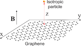
Figure 1: System of suspended graphene and an isotropic particle at a distance $z$, in presence of a perpendicular static magnetic field.

However, the possibility of controlling the Casimir-Polder interaction between an atom and a graphene sheet by an external agent has never been envisaged so far. The possibility of varying the atom-graphene interaction without changing the physical system would be extremely appealing for both experiments and applications. With this motivation, and exploring the extraordinary magneto-optical response of graphene, in the present work we investigate the Casimir-Polder interaction between a Rubdium atom and a suspended graphene sheet under the influence of an external magnetic field ${\bf B}$. We show that just by changing the applied magnetic field, the atom-graphene interaction can be greatly reduced, up to $80\%$ of its value without the field. Furthermore, we demonstrate that at low temperatures ($T\simeq 4$ K) the Casimir-Polder energy exhibits sharp discontinuities at certain values of $B$, that we show to be a manifestation of the quantum Hall effect. As the distance $z$ between the atom and the graphene sheet grows to $z\gtrsim 1\ \mu$m, these discontinuities form a plateau-like pattern with quantized values for the Casimir-Polder energy. We also show that at room temperature ($T\simeq 300$ K) thermal effects must be taken into account even for considerably short distances. Moreover, in this case the discontinuities in the atom-graphene interaction do not occur, although the Casimir-Polder energy can still be tuned in $\sim 50\%$ by applying an external magnetic field.

Let us consider that an isotropic particle is placed at a distance $z$ above a suspended graphene sheet biased by a static magnetic field ${\bf B}=B\hat{{\bf z}}$, as depicted in Fig. 1. The whole system is assumed to be in thermal equilibrium at temperature $T$. When $B\neq 0$ the optical properties of graphene can be well described in terms of a homogeneous but anisotropic two-dimensional conductivity tensor. In this case, the Casimir-Polder (CP) energy interaction can be calculated trough the scattering approach and can be cast as Paulo1

$$U_{T}(z) = \frac{k_{B}T}{\varepsilon_{0}c^{2}}{\sum_{l=0}^{\infty}}^{\prime}\xi_{l}^{2}\,\alpha(i\xi_{l})\int\frac{d^{2}\textbf{k}}{(2\pi)^{2}}\frac{e^{-2\kappa_{l}z}}{2\kappa_{l}}$$ (3)

$$\times\Bigg{[}r^{s,s}(\textbf{k},i\xi_{l},B)-\Bigg{(}1+\frac{2c^{2}k^{2}}{\xi_{l}^{2}}\Bigg{)}r^{p,p}(\textbf{k},i\xi_{l},B)\Bigg{]}\,,$$

where $\xi_{l}=2\pi l/(\hbar k_{B}T)$ are the so called Matsubara frequencies, $\kappa_{n}=\sqrt{\xi_{l}^{2}/c^{2}+k^{2}}$, $\alpha(i\xi)$ is the electric polarizability of the particle, and $r^{s,s}(\textbf{k},i\xi,B)$, $r^{p,p}(\textbf{k},i\xi,B)$ are the diagonal reflection coefficients associated to graphene. As usual, the prime in the summation means that the zero-th term has to be weighted by a factor of 1/2. Note that the cross-polarization reflection coefficients $r^{s,p}(\textbf{k},i\xi,B)$ and $r^{p,s}(\textbf{k},i\xi,B)$, despite being non-vanishing, do not appear in (3). This, however, does not mean that anisotropy plays no role in the interaction energy, as transverse conductivities/permittivities could still appear in $r^{s,s}(\textbf{k},i\xi,B)$, $r^{p,p}(\textbf{k},i\xi,B)$. In particular, by modeling graphene as a $2$-D material with a surface density current ${\bf K}=\mbox{{${\sigma}$}}\cdot{\bf E}|_{z=0}$ and applying the appropriate boundary conditions to the electromagnetic field, one can show that the reflection coefficients are Macdonald_PRL

$$r^{s,s}({\bf k},i\xi,B)=$$

$$\hskip 10.0pt\dfrac{2\sigma_{xx}(i\xi,B)Z^{h}+\eta_{0}^{2}[\sigma_{xx}(i\xi,B)^{2}+\sigma_{xy}(i\xi,B)^{2}]}{-\Delta({\bf k},i\xi,B)}\,,$$ (4)

$$r^{p,p}({\bf k},i\xi,B)=$$

$$\hskip 10.0pt\dfrac{2\sigma_{xx}(i\xi,B)Z^{e}+\eta_{0}^{2}[\sigma_{xx}(i\xi,B)^{2}+\sigma_{xy}(i\xi,B)^{2}]}{\Delta({\bf k},i\xi,B)}\,,$$ (5)

$$\Delta({\bf k},i\xi,B)=[2+Z^{h}\sigma_{xx}(i\xi,B)][2+Z^{e}\sigma_{xx}(i\xi,B)]$$

$$\hskip 10.0pt+[\eta_{0}\sigma_{xy}(i\xi,B)]^{2}\,,$$ (6)

where $Z^{h}=\xi\mu_{0}/\kappa$, $Z^{e}=\kappa/(\xi\epsilon_{0})$, and $\eta_{0}^{2}=\mu_{0}/\epsilon_{0}$. Besides, $\sigma_{xx}(i\xi,B)$ and $\sigma_{xy}(i\xi,B)$ are the longitudinal and transverse conductivities of graphene, respectively.

The electric conductivity tensor of graphene under an external magnetic field is well known and reads Gusynin

$$\sigma_{xx}(i\xi,B) = \dfrac{e^{3}v_{F}^{2}B\hbar(\xi+\tau^{-1})}{\pi c}\sum\limits_{n=0}^{\infty}\Bigg{\{}\dfrac{n_{F}(M_{n})-n_{F}(M_{n+1})+n_{F}(-M_{n+1})-n_{F}(-M_{n})}{D_{n}(M_{n+1}-M_{n})}+(M_{n}\to-M_{n})\Bigg{\}}\,,$$ (7)

$$\sigma_{xy}(i\xi,B) = \dfrac{e^{3}v_{F}^{2}B}{-\pi c}\sum\limits_{n=0}^{\infty}\{n_{F}(M_{n})-n_{F}(M_{n+1})-n_{F}(-M_{n+1})+n_{F}(-M_{n})\}\Bigg{[}\dfrac{1}{D_{n}}+(M_{n}\to-M_{n})\Bigg{]}\,,$$ (8)

where $1/\tau$ is a phenomenological scattering rate, $n_{F}(E)$ is the Fermi-Dirac distribution, $D_{n}=(M_{n+1}-M_{n})^{2}+\hbar^{2}(\xi+\tau^{-1})^{2}$, $M_{n}=\sqrt{n}M_{1}$ are the Landau energy levels, $M_{1}^{2}=2\hbar eBv_{F}^{2}/c$ is the Landau energy scale and $v_{F}\simeq 10^{6}$ m/s is the Fermi velocity. Also, in the following we use $\tau=1.84\times 10^{-13}$ s and set the chemical potential at $\mu_{c}=0.115$ eV.

We still have to specify the particle in our setup. It turns out that a Rubidium atom is a convenient choice, since there are experimental data on its complex electric polarizability $\alpha(\omega)$ for a wide range of frequencies Rubidium . As it is clear from (3), we actually need the polarizability evaluated at imaginary frequencies, which can be readily be obtained from the Kramers-Kronig relations provided one has the data for ${\rm Im}\,\alpha(\omega)$ Paulo1 .

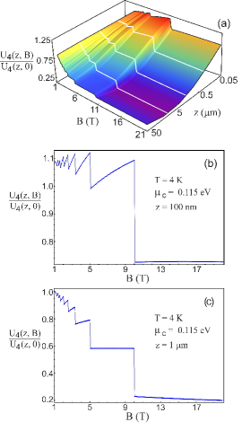
Figure 2: Above: The Casimir-Polder energy of a Rubidium atom in front of a graphene sheet subjected to a magnetic field $B$, as a function of $B$ and the distance $z$. Below: The Casimir-Polder energy as a function of $B$ for two fixed distances: (b) $z=100$ nm, and (c) $z=1$ $\mu$m. In all plots $\mu_{c}=0.115$ eV, $T=4$ K and we have normalized $U_{4}(z,B)$ by the energy in the absence of magnetic field $U_{4}(z,0)$.

Our first results are summarized in Fig. 2a, where we depict the CP energy of our setup as a function of the atom-graphene distance $z$ and magnetic field $B$ for $T=4$ K (normalized by its corresponding value for $B=0$ T). The hallmark of this plot is, surely, the great amount of discontinuities shown by the energy as a function of $B$ for all distances considered. These drops show up even more clearly in Figs. 2b and 2c, where we take two cuts of Fig. 2a at two different fixed values of $z$, namely $z=100$ nm and $z=1$ $\mu$m, and present them as 2-D plots. Such discontinuities are directly linked to the discrete Landau levels brought about by the application of a magnetic field. In order to understand the situation, let us consider the energy-momentum dispersion diagram of graphene in the presence of a static magnetic field depicted in Fig. 3. On the left the usual linear dispersion relation of graphene is presented by the blue solid line. Due to the magnetic field the carriers in graphene can occupy only the discrete values of energy, given by the Landau levels $M_{n}$ represented by black dots. The allowed transitions between two Landau levels give rise to all terms of the summations in Eqs. (7) and (8). There are two kinds of transitions: interband transitions, that connect levels at distinct bands (e. g. long arrow between $-M_{n_{c}}$ and $M_{n_{c}+1}$), and intraband transitions that involve levels at the same band (e. g. short arrow between $M_{n_{c}}$ and $M_{n_{c}+1}$). The possibility of occurrence of a specific transition is related to the difference between the probabilities of having the initial and final levels full and empty, respectively. Ultimately, these probabilities are given by the Fermi-Dirac distribution (solid orange line on the right of Fig. 3). Hence whenever a given Landau level, whose position in energy depends on $B$, crosses upwards (downwards) the chemical potential (dot-dashed green line) of the graphene sheet, it gets immediately depopulated (populated) as a consequence of the quasi-step-function character of the Fermi-Dirac distribution at 4 K. Therefore the crossing of the $n$-th level sharply quenches the $M_{n}\leftrightarrow M_{n+1}$ transition; at the same time that it gives birth to the $M_{n-1}\leftrightarrow M_{n}$ one Gusynin , in a process that changes the conductivity, and thus the interaction energy, discontinuously. The fact that the CP energy always drops down at a discontinuity as we increase $B$ may be understood by recalling the behavior of the relativistic Landau levels with $\sqrt{n}$ (see above). This square-root growth implies that the $n-1$ $\leftrightarrow$ $n$ gap is wider than the $n$ $\leftrightarrow$ $n+1$ one, making the transition weaker, hence reducing the overall conductivity. A similar analysis is valid for the interband transitions.

Figure 2 also reveals that a flattening of the steps in the CP energy between drops occurs as $B$ increases. However, if on the one hand for $z=100$ nm only the very last step is really flat, on the other hand many plateau-like steps exist for $z=1$ $\mu$m. This result is connected to the electrostatic limit of the conductivity: for large distances the exponential factor in (3) strongly suppress all contributions coming from $l\neq 0$, whereas for $l=0$ and large magnetic fields $\sigma_{xx}\sim 0$ and $\sigma_{xy}\sim\pm(2N+1)e^{2}/(\pi\hbar)$, where $N$ is an integer Graphene . Therefore, in the limit of large distances (of the order of micrometers) only the Hall conductivity contributes to $U_{4}(z,B)$, and the CP energy became almost quantized Macdonald_PRL . Furthermore, one should note the striking reduction in the force as we sweep through different values of $B$. While for $z=100$ nm this reduction can be as hight as $30\%$, one can get up to an impressive $80\%$ decrease in the CP interaction for $z=1$ $\mu$m and $B\gtrsim$ 10 T, with huge drops in between. Finally, it should be remarked that for $B\gtrsim$ 10 T the CP interaction is practically insensitive to changes in the magnetic field, regardless of the atom-graphene distance. In this regime the discontinuities in the CP energy do not occur any longer. This effect has its origins in the fact that there is a critical value of the magnetic field $B_{c}$ (in the present case, $B_{c}\sim 10$ T) for which the transition $M_{0}\rightarrow M_{1}$ is dominant since all Landau levels, except $M_{0}$, are above the chemical potential. Altogether, our findings suggest that the atom-graphene is a particularly suited system for investigation of the effects of external magnetic fields on CP forces, and may pave the way for an active modulation of dispersion forces in general.

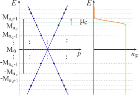
Figure 3: Left: energy-momentum dispersion diagram of graphene in a magnetic field. The blue lines show the usual linear dispersion relation of graphene whilst the Landau levels brought forth by the introduction of $B$ are represented by the black dots. The long (short) vertical arrow shows the lowest energy interband (intraband) transition crossing the chemical potential (dot-dashed green line). Right: Fermi-Dirac distribution at temperature $T$.

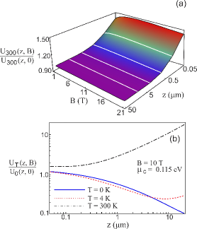
Figure 4: Above: the Casimir-Polder interaction energy $U_{300}(z,B)$ (normalized by $U_{300}(z,0)$) between a Rubidium atom and a graphene sheet as a function of both distance and external magnetic field strength for $T=300$ K. Below: the Casimir-Polder energy (normalized by $U_{0}(z,0)$) as a function of the mutual distance between atom and graphene sheet for $T=0$ K (solid line), $T=4$ K (dashed line), and $T=300K$ (dot-dashed line). In both panels (a) and (b) the graphene chemical potential is $\mu_{c}=0.115$ eV.

In order to investigate thermal effects, Fig. 3a we present the CP energy as a function of both $z$ and $B$ at room temperature. The most distinctive aspect of Fig. 3a is the complete absence of discontinuities that characterize the behavior of the CP energy at low temperatures. At $T=300$ K the Fermi-Dirac distribution is a quite smooth function of the energy levels, allowing for a partial filling of many Landau levels. Hence the effects of the crossing between these levels and the graphene’s chemical potential is hardly noticed, resulting in a smooth CP energy profile. Another important aspect of Fig. 3a is that the CP energy becomes essentially independent of $B$ for $z\gtrsim 1$ $\mu$m. For this set of parameters, the system is already in the thermal regime, where the CP energy is essentially dominated by the electrostatic conductivity. In this regime, the CP energy is very weakly affected by variations in $B$ due the already discussed exponential suppression of the $l\geq 1$ terms in Eq. (3). We emphasize, however, that the absence of discontinuities does not prevent one from tuning the CP interaction between a Rb atom and a graphene sheet at least at short distances. This tunability can be achieved even for relatively modest magnetic fields, as the value of the CP energy can increase up to 50 $\%$ (compared to the case where $B=0$ T) by applying a magnetic field of $B=5$ T for $z=50$ nm. For $B=5$ T and $z=100$ nm, the variation in the interaction can still be as high as 30$\%$. In Fig. 3b the CP energy is calculated for $B=10$ T and for different temperature values, $T=0$, $4$, and $300$ K, all normalized by the zero-temperature, zero-field energy value $U_{0}(z,0)$. Figure 3b reveals that thermal corrections are relevant even for low temperatures, and for a broad range of distances: we have a 10-20% variation in the relative difference of $U_{4}(z,10)$ and $U_{0}(z,10)$ in the 1-10 $\mu$m interval, which is in the ballpark of recent/current experiments’ precision. Besides, Fig. 3b demonstrates that at room temperature not only the thermal effects are absolutely dominant in the micrometer range, but they also play an important role even for small distances. Indeed, at $z=100$ nm the relative difference between $U_{300}(z,10)$ and $U_{0}(z,10)$ is $\sim 45\%$ and at $z=1$ $\mu$m it is $\sim 400\%$; so in the latter approximately $80\%$ of the CP energy come from thermal contribution. We conclude that, at room temperature, these effects should be taken into account for a wide range of distances between the atom and the graphene sheet.

In conclusion, we have investigated the dispersive Casimir-Polder interaction between a Rubidium atom and a suspended graphene sheet subjected to an external magnetic field ${\bf B}$. Apart from providing a concrete physical system where the dispersive interaction in nano and micrometer scales can be controlled by an external agent, we show that just by changing the applied magnetic field, this interaction can be reduced up to $80\%$ of its value in the absence of the field. Further, due to the quantum Hall effect, we show that for low temperatures the Casimir-Polder interaction energy acquires sharp discontinuities at given values of $B$ and that these discontinuities approach a plateau-like pattern with a quantized Casimir-Polder interaction energy as the atom and the graphene sheet become more and more far apart. In addition, we show that at room temperature thermal effects must be taken into account even for considerably short distances. In this case, the discontinuities in the atom-graphene dispersive interaction are not present any longer, although the interaction can still be tuned in $\sim 50\%$ by applying an external magnetic field.

We thank P. A. Maia Neto for assistance with the Rubidium data, and R. S. Decca, I. V. Fialkovsky, E. C. Marino, and N. M. R. Peres for useful discussions. We also acknowledge CNPq and FAPERJ for partial financial support.

References

- (1) R. Eisenschitz and F. London, Z. Phys. 60, 491 (1930); F. London, Z. Phys. 63, 245 (1930).
- (2) H. B. G. Casimir and D. Polder, Nature 158, 787 (1946).
- (3) H.B.G. Casimir, and D. Polder, Phys. Rev. 73, 360 (1948).
- (4) J. E. Lennard-Jones, Trans. Faraday Soc. 28, 333–359 (1932).
- (5) P. W. Milonni, The Quantum Vacuum: An Introduction to Electrodynamics, (Academic Press, San Diego, CA, 1994).
- (6) D. P. Craig and T. Thirunamachandran, Molecular Quantum Electrodynamics, (Dover, New York, 1998).
- (7) S. Y. Buhmann, and D-G. Welsh, Prog. Quant. Elect., 31, 51 (2008).
- (8) G. L. Klimchitskaya, U. Mohideen, and V.M. Mostepanenko, Rev. Mod. Phys. 81, 1827 (2009).
- (9) M. Bordag, G. L. Klimchitskaya, U. Mohideen, and V. M. Mostepanenko, Advances in the Casimir Effect, (Oxford U.P., Oxford, 2009).
- (10) D. Dalvit, P. Milonni, D. Roberts, F. S. S. Rosa (eds.) Casimir Physics, Lecture Notes in Physics Vol. 834, Springer (2010).
- (11) S. Y. Buhmann, Dispersion Forces I - Macroscopic Quantum Electrodynamics and Ground-State Casimir, Casimir–Polder and van der Waals Forces, (Springer, Heidelberg, 2013); S. Y. Buhmann, Dispersion Forces II - Many-Body Effects, Excited Atoms, Finite Temperature and Quantum Friction, (Springer, Heidelberg, 2013).
- (12) C. I. Sukenik, M. G. Boshier, D. Cho, V. Sandoghdar, and E. A. Hinds, Phys. Rev. Lett. 70, 560 (1993).
- (13) A. Landragin, J.-Y. Courtois, G. Labeyrie, N. Vansteenkiste, C. I. Westbrook, and A. Aspect, Phys. Rev. Lett. 77, 1464 (1996).
- (14) F. Shimizu, Phys. Rev. Lett. 86, 987 (2001).
- (15) V. Druzhinina, and M. DeKieviet, Phys. Rev. Lett. 91, 193202 (2003).
- (16) T. A. Pasquini, Y. Shin, C. Sanner, M. Saba, A. Schirotzek, D. E. Pritchard, and W. Ketterle, Phys. Rev. Lett. 93, 223201 (2004).
- (17) J. M. Obrecht, R. J. Wild, M. Antezza, L. P. Pitaevskii, S. Stringari, and E. A. Cornell, Phys. Rev. Lett. 98, 063201 (2007).
- (18) A. Laliotis, T. P. de Silans, I. Maurin, M. Ducloy, D. Bloch, Nature Commun. 5, 4364 (2014).
- (19) E. M. Lifshitz, Zh. Eksp. Teor. Fiz. 29, 94 (1955), translated in Sov. Phys. JETP 2, 73 (1956).
- (20) I.E. Dzyaloshinskii and L.P. Pitaevskii, Sov. Phys. JETP 9, 1282 (1959); I.E. Dzyaloshinskii, E.M. Lifshitz, and L.P. Pitaevskii, Adv. Phys. 10, 165 (1961).
- (21) K. Autumn, M. Sitti, Y. A. Liang, A. M. Peattle, W. R. Hansen, S. Sponberg, T. W. Kenny, R. Fearing, J. N. Israelachvili, and R. J. Full, Proc. Natl. Acad. Sci. U.S.A. 99, 12252 (2002).
- (22) J. Klimes and A. Michaelides, J. Chem. Phys. 137, 120901 (2012).
- (23) K. A. Milton, J. Phys. A 24, R209 (2004).
- (24) S. K. Lamoreaux, Rep. Prog. Phys. 68, 201 (2005).
- (25) A. B. C Neto, F. Guinea, N. M. R. Peres, K. S. Novoselov and A. K. Geim, Rev. Mod. Phys. 81, 109 (2009); N. M. R. Peres, Rev. Mod. Phys. 82, 2673 (2010).
- (26) M. Bordag, I.V. Fialkovsky, D.M. Gitman and D.V. Vassilevich, Phys. Rev. B 80, 245406 (2009).
- (27) G. Gómez-Santos, Phys. Rev. B 80, 245424 (2009).
- (28) V. Svetovoy, Z. Moktadir, M. Elwenspoek and H. Mizuta, Europhys. Lett. 96, 14006 (2011).
- (29) I.V. Fialkovsky, V.N. Marachevsky and D.V. Vassilevich, Phys. Rev. B 84, 035446 (2011).
- (30) D. Drosdoff and L.M. Wooks, Phys. Rev. A 84, 062501 (2011).
- (31) B.E. Sernelius, Phys. Rev. B 85, 195427 (2012).
- (32) M. Bordag, G.L. Klimchitskaya and V.M. Mostepanenko, Phys. Rev. B 86, 165429 (2012).
- (33) G.L. Klimchitskaya and V.M. Mostepanenko, Phys. Rev. B 87, 075439 (2013).
- (34) G. L. Klimchitskaya and V. M. Mostepanenko, Phys. Rev. B 89, 035407 (2014).
- (35) W.-K. Tse and A. H. MacDonald, Phys. Rev. Lett. 109, 236806 (2012).
- (36) Yu V. Churkin, A. B. Fedortsov, G. L. Klimchitskaya and V. A. Yurova, Phys. Rev. B 82, 165433 (2010).
- (37) T. E. Judd, R.G. Scott, A.M. Martin, B. Kaczmarek and T.M. Frohold, New J. Phys.13, 083020 (2011).
- (38) M. Chaichian, G. L. Klimchitskaya, V. M. Mostepanenko and A. Tureanu, Phys. Rev. A 86, 012515 (2012).
- (39) G. L. Klimchitskaya and V. M. Mostepanenko, Phys. Rev. A 89, 062508 (2014).
- (40) S. Ribeiro and S. Scheel, Phys. Rev. A 88, 042519 (2013); Erratum: Phys. Rev. A 89, 039904 (2014).
- (41) A. M. Contreras-Reyes, R. Guérout, P. A. Maia Neto, D. A. R. Dalvit, A. Lambrecht, and S. Reynaud, Phys. Rev. A 82, 052517 (2010).
- (42) V. P. Gusynin, S. G. Sharapov, and P. Cabotte, J. Phys.: Cond. Mat. 19, 026022 (2007); V. P. Gusynin, and S. G. Sharapov, Phys. Rev. B 73 245511 (2006).
- (43) A. Derevianko, S. G. Porsev, and J. F. Babb, At. Data Nucl. Data Tables 96, 323 (2010).