The $\mu\to e\gamma$ decay in a systematic effective
field theory approach with dimension 6 operators

Abstract

We implement a systematic effective field theory approach to the benchmark process $\mu\to e\gamma$, performing automated one-loop computations including dimension 6 operators and studying their anomalous dimensions. We obtain limits on Wilson coefficients of a relevant subset of lepton-flavour violating operators that contribute to the branching ratio $\mu\to e\gamma$ at one-loop. In addition, we illustrate a method to extract further constraints induced by the mixing of operators under renormalisation-group evolution. This results in limits on the corresponding Wilson coefficients directly at the high scale. The procedure can be applied to other processes as well and, as an example, we consider also lepton-flavour violating decays of the $\tau$.

1 Introduction

The study of lepton-flavour violating (LFV) processes in the charged sector offers a possibility to probe the Standard Model (SM) to very high scales. Of particular importance is the LFV decay $\mu\to e\gamma$. First, there are very impressive experimental limits on this branching ratio. The current best limit ${\rm BR}(\mu^{+}\to e^{+}\gamma)<5.7\times 10^{-13}$ Adam et al. (2013) has been set by the MEG collaboration at PSI and an upgrade of the experiment is underway to improve the sensitivity further by an order of magnitude Baldini et al. (2013). Second, in the SM with neutrino masses $m_{\nu}$ this branching ratio is suppressed by the tiny ratio $(m_{\nu}/m_{W})^{4}$, where $m_{W}$ is the mass of the $W$-boson. Thus, the SM branching ratio is well below any experimental limit that is achievable in the foreseeable future and any positive signal for $\mu\to e\gamma$ would be clear evidence for physics beyond the Standard Model (BSM). Conversely, improving limits on this branching ratio would put even more serious constraints on many BSM models. Given its importance the decay $\mu\to e\gamma$ has been studied in a large number of explicit BSM models. Here, a more model independent approach is taken.

The impact of a BSM model with new physics at a large energy scale $\Lambda\gg m_{W}$ to observables at much smaller scales can be described using an effective field theory (EFT) approach. The SM is considered to be an EFT valid up to a scale $\Lambda$ and the BSM effects at lower energies are described by operators of dimension $n>4$, suppressed by powers of $\Lambda$. These operators are generated from the BSM physics by integrating out the heavy non-SM degrees of freedom. In general, the dominant effects are expected to come from dimension 5 and dimension 6 operators. A minimal list of all possible such operators formed from SM fields only and respecting the $SU(3)\times SU(2)\times U(1)$ gauge invariance consists of one dimension 5 operator Weinberg (1979) and 64 dimension 6 operators Buchmuller and Wyler (1986); Grzadkowski et al. (2010), five of which are baryon number violating. As many of these operators actually represent matrices in generation space, the total number of coefficients needed to describe the most general case is rather large. Nevertheless, this is a systematic approach to study the impact of BSM physics to a large class of observables obtained from experiments at very different energy scales. It is used in Higgs physics, B-physics and the study of electric dipole moments to mention just a few of the applications.

Applying these ideas to the flavour changing decay $\mu\to e\gamma$ we note that there is a dimension 6 operator ($Q_{e\gamma}$ to be defined below) that induces such a decay directly at tree level. It is clear that the MEG limit provides an extremely strong constraint on the coefficient of this operator. However, such a decay can also be induced indirectly from other operators that are not immediately linked to $\mu\to e\gamma$. Thus, even if a particular BSM does not induce the operator $Q_{e\gamma}$ at the high scale $\Lambda$, it can lead to a non-vanishing contribution to $\mu\to e\gamma$. Broadly speaking, this can happen in two different ways.

First, some dimension 6 operators other than $Q_{e\gamma}$ can induce a decay $\mu\to e\gamma$ beyond tree level. The contribution to $\mu\to e\gamma$ from dimension 6 operators at one loop has partially been computed Crivellin et al. (2014a) and it has been found that several operators contribute. This can lead to very serious independent constraints on the coefficients of these operators.

The second possibility is through mixing in the renormalisation-group (RG) evolution of the Wilson coefficient $C_{e\gamma}$ of the operator $Q_{e\gamma}$. The Wilson coefficients $C_{i}(\Lambda)$ of the higher-dimensional operators are determined at the high scale $\Lambda$ by integrating out the heavy fields. If these coefficients then are to be used to study the impact of the higher-dimensional operators to observables at a lower scale $\lambda$, say $\lambda\sim m_{W}$, the coefficients $C_{i}(m_{W})$ have to be determined from $C_{i}(\Lambda)$ through RG evolution. The one-loop RG evolution of the dimension 6 operators has been studied Jenkins et al. (2013, 2014); Alonso et al. (2014) and, as expected, it has been found that other operators mix with $Q_{e\gamma}$ under the evolution.

The aim of this paper is to present a complete analysis of $\mu\to e\gamma$ in the context of an EFT approach including dimension 6 operators. To this end, we repeat and extend the one-loop calculation presented in Crivellin et al. (2014a) for this process with a RG analysis. The RG running is done in two steps. We first evolve from the large scale $\Lambda$ to the electroweak scale $m_{V}\sim m_{W}\sim m_{Z}$ and then use a modified evolution suitable for the scales $m_{\mu}\lesssim\lambda\lesssim m_{Z}$, where the mass of the muon, $m_{\mu}$, is the scale at which the coefficient $C_{e\gamma}$ has to be evaluated for the process $\mu\to e\gamma$. We consider the subset of all dimension 6 operators that are most directly linked to the LFV decay. The details of the Lagrangian and the setup for the calculations are given in Section 2. In Section 3 the relation between the Lagrangian and the branching ratio is discussed. Section 4 is the main part of the paper. Section 4.1 starts with the one-loop result of the branching ratio computed in the EFT. The experimental limit on the branching ratio can be translated directly into a limit for $C_{e\gamma}(m_{\mu})$. From the explicit one-loop results, it is also possible to extract limits on other Wilson coefficients evaluated at the small scale. In a second step, in Section 4.2, the anomalous dimensions of the operator $Q_{e\gamma}$ and those operators that mix with $Q_{e\gamma}$ are computed. These results are then used to obtain limits on the Wilson coefficients of these operators, evaluated directly at the large scale $\Lambda$. Our conclusions are presented in Section 5. The details of the renormalisation needed for the one-loop result and the anomalous dimensions are given in Appendix A. In Appendix B the result for the (unrenormalised) one-loop branching ratio is listed. Finally, in Appendix C we apply the same method to the LFV decays of the $\tau$ to obtain limits on the corresponding Wilson coefficients.

2 Effective D-6 extension of the SM: leptonic interactions

In this paper we take the point of view that the SM is an EFT valid up to some large scale $\Lambda$ and BSM physics can be parametrised by operators of dimension 6 (D-6). Higher dimensional operators are not considered. A complete list of gauge invariant D-6 operators has been given, in Grzadkowski et al. (2010). In this section the subset of D-6 operators that are relevant for our analysis of $\mu\to e\gamma$ is presented and the implementation of these operators in automated computational tools is also briefly discussed.

$\psi^{2}X\varphi$		$\psi^{2}\varphi^{2}D$		$\psi^{2}\varphi^{3}$
$Q_{eW}$	$(\bar{l}_{p}\sigma^{\mu\nu}e_{r})\tau^{I}\varphi W_{\mu\nu}^{I}$	$Q_{\varphi l}^{(1)}$	$(\mbox{${\varphi^{\dagger}i\,\raisebox{5.69054pt}{\boldmath${}^{\leftrightarrow}$}D_{\mu}\,\varphi}$})(\bar{l}_{p}\gamma^{\mu}l_{r})$	$Q_{e\varphi}$	$(\varphi^{\dagger}\varphi)(\bar{l}_{p}e_{r}\varphi)$
$Q_{eB}$	$(\bar{l}_{p}\sigma^{\mu\nu}e_{r})\varphi B_{\mu\nu}$	$Q_{\varphi l}^{(3)}$	$(\mbox{${\varphi^{\dagger}i\,\raisebox{5.69054pt}{\boldmath${}^{\leftrightarrow}$}D_{\mu}^{\,I}\,\varphi}$})(\bar{l}_{p}\tau^{I}\gamma^{\mu}l_{r})$
		$Q_{\varphi e}$	$(\mbox{${\varphi^{\dagger}i\,\raisebox{5.69054pt}{\boldmath${}^{\leftrightarrow}$}D_{\mu}\,\varphi}$})(\bar{e}_{p}\gamma^{\mu}e_{r})$

Table 1: D-6 operators consisting of fermions and bosons, according to Grzadkowski et al. (2010).

$(\bar{L}L)(\bar{L}L)$		$(\bar{R}R)(\bar{R}R)$		$(\bar{L}L)(\bar{R}R)$		$(\bar{L}R)(\bar{R}L)$ and $(\bar{L}R)(\bar{L}R)$
$Q_{ll}$	$(\bar{l}_{p}\gamma_{\mu}l_{r})(\bar{l}_{s}\gamma^{\mu}l_{t})$	$Q_{ee}$	$(\bar{e}_{p}\gamma_{\mu}e_{r})(\bar{e}_{s}\gamma^{\mu}e_{t})$	$Q_{le}$	$(\bar{l}_{p}\gamma_{\mu}l_{r})(\bar{e}_{s}\gamma^{\mu}e_{t})$	$Q_{ledq}$	$(\bar{l}_{p}^{j}e_{r})(\bar{d}_{s}q_{t}^{j})$
$Q_{lq}^{(1)}$	$(\bar{l}_{p}\gamma_{\mu}l_{r})(\bar{q}_{s}\gamma^{\mu}q_{t})$	$Q_{eu}$	$(\bar{e}_{p}\gamma_{\mu}e_{r})(\bar{u}_{s}\gamma^{\mu}u_{t})$	$Q_{lu}$	$(\bar{l}_{p}\gamma_{\mu}l_{r})(\bar{u}_{s}\gamma^{\mu}u_{t})$	$Q_{lequ}^{(1)}$	$(\bar{l}_{p}^{j}e_{r})\varepsilon_{jk}(\bar{q}_{s}^{k}u_{t})$
$Q_{lq}^{(3)}$	$(\bar{l}_{p}\gamma_{\mu}\tau^{I}l_{r})(\bar{q}_{s}\gamma^{\mu}\tau^{I}q_{t})$	$Q_{ed}$	$(\bar{e}_{p}\gamma_{\mu}e_{r})(\bar{d}_{s}\gamma^{\mu}d_{t})$	$Q_{ld}$	$(\bar{l}_{p}\gamma_{\mu}l_{r})(\bar{d}_{s}\gamma^{\mu}d_{t})$	$Q_{lequ}^{(3)}$	$(\bar{l}_{p}^{j}\sigma_{\mu\nu}e_{r})\varepsilon_{jk}(\bar{q}_{s}^{k}\sigma^{\mu\nu}u_{t})$
				$Q_{qe}$	$(\bar{q}_{p}\gamma_{\mu}q_{r})(\bar{e}_{s}\gamma^{\mu}e_{t})$

Table 2: D-6 operators consisting of four fermions, according to Grzadkowski et al. (2010).

The Lagrangian considered in this paper is the SM Lagrangian $\mathcal{L}_{\rm SM}$ extended by D-6 operators

$$\mathcal{L}=\mathcal{L}_{\rm SM}+\frac{1}{\Lambda^{2}}\sum_{i}C_{i}\,Q_{i},$$ (2.1)

where the sum is over the D-6 operators listed in Tables 1 and 2. These are the D-6 operators that can cause LFV interactions. The dimension 5 operator is not included in Eq. (2.1): since the effect of this operator on $\mu\to e\gamma$ transitions has been studied before Petcov (1977); Minkowski (1977) we do not consider it in our analysis. The notation and conventions are taken from Grzadkowski et al. (2010). In particular, $\{p,r,s,t\}$ denote generation indices. In the Lagrangian the operators appear multiplied by $C_{i}^{pr\ldots}/\Lambda^{2}$, where $C_{i}^{pr\ldots}$ are dimensionless coefficient matrices with two or four generation indices. With regard to the Hermitian conjugation, it is worth to remark that

• in the operator class $\psi^{2}\varphi^{2}D$, it is self-realised by transposition of generation indices;

• in the operator classes $(\bar{L}L)(\bar{L}L)$, $(\bar{R}R)(\bar{R}R)$ and $(\bar{L}L)(\bar{R}R)$, it is self-realised by transposition of generation indices once the prescription $C^{prst}=C^{rpts}$ is assumed;

• for the other operator classes, adding the Hermitian conjugate (not listed explicitly in Tables 1 and 2) is understood.

Working in the physical basis rather than in the gauge basis, the two operators of the $\psi^{2}X\varphi$ set are rewritten using

$$Q_{eB} \rightarrow Q_{e\gamma}c_{W}-Q_{eZ}s_{W},$$ (2.2)

$$Q_{eW} \rightarrow-Q_{e\gamma}s_{W}-Q_{eZ}c_{W},$$ (2.3)

where $s_{W}=\sin(\theta_{W})$ and $c_{W}=\cos(\theta_{W})$ are the sine and cosine of the weak mixing angle. The term

$$\mathcal{L}_{e\gamma}\equiv\frac{C_{e\gamma}}{\Lambda^{2}}Q_{e\gamma}+\mbox{h.c.}=\frac{C_{e\gamma}^{pr}}{\Lambda^{2}}(\bar{l}_{p}\sigma^{\mu\nu}e_{r})\varphi F_{\mu\nu}+\mbox{h.c.},$$ (2.4)

where $F_{\mu\nu}$ is the electromagnetic field-strength tensor, is then the only term in the D-6 Lagrangian that induces a $\mu\to e\gamma$ transition at tree level. However, at one loop (and even higher order) the other operators listed in Tables 1 and 2 also potentially contribute.

Finally, special attention is devoted to the operator $Q_{e\varphi}$: in Feynman gauge, the presence of such an operator produces Lagrangian terms of the form

$$\mathcal{L}_{e\varphi}= \frac{v^{3}}{2\sqrt{2}\Lambda^{2}}C_{e\varphi}^{pr}\bar{e}_{p}e_{r}+\frac{3v^{2}}{2\sqrt{2}\Lambda^{2}}C_{e\varphi}^{pr}\bar{e}_{p}e_{r}h$$

$$+ i\frac{v^{2}}{2\sqrt{2}\Lambda^{2}}C_{e\varphi}^{pr}\bar{e}_{p}e_{r}\widehat{Z}+i\frac{v^{2}}{2\Lambda^{2}}C_{e\varphi}^{pr}\bar{e}_{p}\nu_{r}\widehat{W}^{+}+\left[\dots\right].$$ (2.5)

Apparently, this operator introduces Goldstone-boson ($\widehat{Z},\ \widehat{W}^{\pm}$) interactions which are not compensated by any analogous vectorial term. However, the combination of Eq. (2) with the D-4 SM Yukawa terms gives

$$\mathcal{L}_{\rm Yukawa}+\mathcal{L}_{e\varphi}= \frac{v}{\sqrt{2}}\left(-y_{pr}+\frac{v^{2}}{2\Lambda^{2}}C_{e\varphi}^{pr}\right)\bar{e}_{p}e_{r}$$

$$+ \frac{1}{\sqrt{2}}\left(-y_{pr}+\frac{v^{2}}{2\Lambda^{2}}C_{e\varphi}^{pr}\right)\bar{e}_{p}e_{r}h+\frac{v^{2}}{\sqrt{2}\Lambda^{2}}C_{e\varphi}^{pr}\bar{e}_{p}e_{r}h$$

$$+ \frac{i}{\sqrt{2}}\left(-y_{pr}+\frac{v^{2}}{2\Lambda^{2}}C_{e\varphi}^{pr}\right)\bar{e}_{p}e_{r}\widehat{Z}+i\left(-y_{pr}+\frac{v^{2}}{2\Lambda^{2}}C_{e\varphi}^{pr}\right)\bar{e}_{p}\nu_{r}\widehat{W}^{+}+\left[\dots\right].$$ (2.6)

From Eq. (2), it is understood that any 3-point off-diagonal interaction involving Goldstone bosons is not physical, i.e. it can be removed by an orthogonal transformation. However, this procedure results in

• a residual term with a physical Higgs supporting LFV currents;

• a redefinition of the relation between leptonic Yukawa couplings and leptonic masses:

  $$y_{pp}\rightarrow\frac{\sqrt{2}m_{p}}{v}+\frac{v^{2}}{2\Lambda^{2}}C_{e\varphi}^{pp}.$$ (2.7)

In the framework of LFV processes at tree level and one loop, the prescription of Eq. (2.7) is never relevant. However, it is of fundamental importance in the case of flavour diagonal interactions and related analyses such as the study of the anomalous magnetic moment of the muon $(g-2)_{\mu}$.

In the following sections, one-loop calculations in the theory given by the Lagrangian Eq. (2.1) will be presented. In order to perform such calculations in an automated way, several openly available tools were used:

• in order to obtain consistent Feynman rules, the described model was implemented both in LanHEP v3.1.9 Semenov (2010) and in FeynRules v2.0 Alloul et al. (2014), and the agreement among the two packages was checked;

• in order to produce a model file for the FeynArts v3.9 Hahn (2001) and FormCalc v8.3 Hahn and Perez-Victoria (1999); Chokoufe Nejad et al. (2014) packages, the FeynArts interface of FeynRules was exploited;

• the combined packages FeynArts/FormCalc were employed to generate non-integrated amplitudes to be elaborated afterwards with the symbolic manipulation system Form v4.0 Kuipers et al. (2013).

The list of resulting tree-level Feynman rules from the Lagrangian Eq. (2.1) is too long to be given explicitly in this paper. It will be provided after the publication of this work: it will appear in the FeynRules model database (in the format of a FeynRules model file). However, the Feynman rule for the $\mu-e-\gamma$ interaction (consisting of the effective tree-level interaction plus the one-loop wave-function renormalisation (WFR) of the relevant objects) is presented (see Appendix A).

3 $\mu\to e\gamma$: Branching ratio and constraints

It is well known that in the limit $m_{\mu}\gg m_{e}$ the partial width of the process $\mu\to e\gamma$ is given by

$$\Gamma_{\mu\to e\gamma}=\frac{1}{16\pi m_{\mu}}\left|\mathcal{M}\right|^{2},$$ (3.1)

where $\mathcal{M}$ is the transition amplitude, which contains the model-dependent information. Computing $\mathcal{M}$ in the theory given by Eq. (2.1) and confronting the corresponding branching ratio ${\rm BR}(\mu^{+}\to e^{+}\gamma)$ with the experimental limit Adam et al. (2013) allows to put constraints on the Wilson coefficients $C_{i}$ of some of the D-6 operators in Eq. (2.1).

To make this connection more explicit we note that the Lagrangian Eq. (2.1) induces flavour-violating interactions $\mu\to e\gamma$ that can be written as

$$V^{\mu}=\frac{1}{\Lambda^{2}}i\sigma^{\mu\nu}\left(C_{TL}\,\omega_{L}+C_{TR}\,\omega_{R}\right)\left(p_{2}\right)_{\nu},$$ (3.2)

where the conventions described in Appendix A are used and $\omega_{L/R}=1\mp\gamma^{5}$. Note that no term $\sim\gamma^{\mu}$ appears in Eq. (3.2) since such a term is forbidden by gauge invariance. $C_{TL}$ and $C_{TR}$ are coefficients of dimension one that depend on the Wilson coefficients of the D-6 operators and on the parameters of the SM. The unpolarised squared matrix element is expressed in terms of them as

$$\left|\mathcal{M}\right|^{2}=\frac{4\left(|C_{TL}|^{2}+|C_{TR}|^{2}\right)m_{\mu}^{4}}{\Lambda^{4}},$$ (3.3)

and the branching ratio is

$${\rm BR}(\mu\to e\gamma)=\frac{\Gamma_{\mu\to e\gamma}}{\Gamma_{\mu}}=\frac{m_{\mu}^{3}}{4\pi\Lambda^{4}\Gamma_{\mu}}\left(|C_{TL}|^{2}+|C_{TR}|^{2}\right)=\frac{48\pi^{2}}{G_{F}^{2}m_{\mu}^{2}}\frac{\left(|C_{TL}|^{2}+|C_{TR}|^{2}\right)}{\Lambda^{4}},$$ (3.4)

where $\Gamma_{\mu}=\left(G_{F}^{2}m_{\mu}^{5}\right)/\left(192\pi^{3}\right)$ is the SM total decay width of the muon. The result Eq. (3.4) is well known in the literature, see e.g. Marciano et al. (2008) and references therein. Confronting this result with the experimental upper limit Adam et al. (2013) established by the MEG collaboration on the $\mu^{+}\to e^{+}\gamma$ transition

$${\rm BR}(\mu^{+}\to e^{+}\gamma)\leq 5.7\cdot 10^{-13},$$ (3.5)

the limit

$$\frac{\sqrt{|C_{TL}|^{2}+|C_{TR}|^{2}}}{\Lambda^{2}}\leq 4.3\cdot 10^{-14}\left[{\rm GeV}\right]^{-1}$$ (3.6)

can be obtained.

At tree level, for the process $\mu^{+}\to e^{+}\gamma$ the coefficients appearing in Eq. (3.6) are given by $C_{TR}^{(0)}=-v\,C^{\mu e}_{e\gamma}/\sqrt{2}$ and $C_{TL}^{(0)}=-v\,(C^{e\mu}_{e\gamma})^{*}/\sqrt{2}$. In what follows, we will instead compute the coefficients for the process $\mu^{-}\to e^{-}\gamma$ where the tree-level results are given by $C_{TR}^{(0)}=-v\,C^{e\mu}_{e\gamma}/\sqrt{2}$ and $C_{TL}^{(0)}=-v\,(C^{\mu e}_{e\gamma})^{*}/\sqrt{2}$. From now on the generation indices will often be dropped and the simplified notation $C_{e\gamma}$ will be used for either $C_{e\gamma}^{\mu e}$ or $C_{e\gamma}^{e\mu}$. Similar remarks apply to $C_{eZ}$ and $C_{e\varphi}$. Applying the constraint Eq. (3.6) then immediately results in a constraint on $C_{e\gamma}$.

It is clear that if the BSM physics is such that the matching at the scale $\Lambda$ produces a sizable coefficient $C_{e\gamma}(\Lambda)$ this will be the dominant effect for ${\rm BR}(\mu\to e\gamma)$. On the other hand it is perfectly possible that the coefficient $C_{e\gamma}(\Lambda)$ is zero or strongly suppressed compared to Wilson coefficients of other D-6 operators. In this case effects of operators that enter $C_{TL}$ and $C_{TR}$ only at one loop can be important.

The result of $C_{TL}$ (or $C_{TR}$) computed at one loop can schematically be written as

$$C_{TL}^{(1)}=-\sqrt{2}v\,\left(C_{e\gamma}\left(1+e^{2}c_{e\gamma}^{(1)}\right)+\sum_{i\neq e\gamma}e^{2}c_{i}^{(1)}\,C_{i}\right),$$ (3.7)

where the electromagnetic coupling $e$ stands for a generic coupling and the coefficients $c_{e\gamma}^{(1)}$ and $c_{i}^{(1)}$ depend on SM parameters such as $m_{Z},m_{l}$ etc. To compute the branching ratio at one loop, apart from wave-function renormalisation also the vacuum expectation value (VEV) $v$ has to be renormalised. Even after this renormalisation, the coefficients $c_{e\gamma}^{(1)}$ and $c_{i}^{(1)}$ in general contain ultraviolet singularities. These singularities have to be absorbed by a renormalisation of the coefficient $C_{e\gamma}$. By choosing a particular scheme for this subtraction, a precise definition of the Wilson coefficient is given. In what follows, the $\overline{\rm MS}$ scheme is used.

In passing, it should be mentioned that for the coefficient $c_{e\gamma}^{(1)}$ also infrared singularities have to be taken into consideration. However, the primary interest of considering one-loop corrections is in the contribution of operators other than $Q_{e\gamma}$ to $C_{TL}$ and $C_{TR}$. The corrections $\sim e^{2}c_{e\gamma}^{(1)}C_{e\gamma}$ only result in a small modification of the limit on $C_{e\gamma}$. Hence these corrections will not be considered in this paper.

The renormalised Wilson coefficients and, therefore, the coefficients $C_{TL}$ and $C_{TR}$ are scale dependent quantities. Hence, Eq. (3.6) should be interpreted as a phenomenological constraint on the Wilson coefficients at the relevant energy scale. While $\lambda\sim m_{\mu}$ is the typical energy scale probed by the MEG experiment, the explicit results presented in the next section will show, that for some of the operators the relevant scale is the electroweak scale $\lambda\sim m_{V}$. In any case, these scales are much lower than $\Lambda$, the natural scale for the Wilson coefficients after integrating out the heavy non-SM fields. To stress this subtlety Eq. (3.6) is rewritten as

$$\left.\frac{\sqrt{|C_{TL}(\lambda)|^{2}+|C_{TR}(\lambda)|^{2}}}{\Lambda^{2}}\right|_{\lambda\ll\Lambda}\leq 4.3\cdot 10^{-14}\left[{\rm GeV}\right]^{-1}.$$ (3.8)

In the next section, the explicit result for the coefficients $C_{TL}$ and $C_{TR}$ of Eq. (3.2) computed in the context of the Lagrangian Eq. (2.1) at the tree level and one-loop level is given. Furthermore, various contributions coming from different operators are separately shown. Afterwards, the RG running of the Wilson coefficients is studied and Eq. (3.8) is applied to obtain bounds on each relevant coefficient at the scale $\Lambda$. These limits provide the most direct link between the low-energy observable ${\rm BR}(\mu\to e\gamma)$ and BSM scenarios within an EFT framework.

4 Results

In this section, analytical results and phenomenological studies concerning the impact of Eq. (3.8) on the Wilson coefficients of D-6 operators in the Lagrangian Eq. (2.1) are presented. The study is split into two parts:

• The complete result for the decay $\mu\to e\gamma$ in the EFT up to the one-loop level is calculated. These results are then used to obtain bounds on the Wilson coefficients of D-6 operators at the fixed scale $\lambda=m_{\mu}$ or $\lambda=m_{V}$, applying the experimental constraint on the branching ratio ${\rm BR}(\mu\to e\gamma)$.

• The mixing of a subset of D-6 operators with $Q_{e\gamma}$ under RG evolution is computed. Translating the experimental constraint on ${\rm BR}(\mu\to e\gamma)$ to a limit on $C_{e\gamma}(m_{Z})$, bounds on Wilson coefficients $C_{i}(\Lambda)$ of operators $Q_{i}$ that mix with $Q_{e\gamma}$ are then obtained. The dependence on $\Lambda$ of these bounds is discussed.

Due to the high level of automation, a certain number of cross checks was strongly required. Unless specified otherwise, every result of this paper was tested under the following aspects:

• with no exceptions, all the calculations were performed in a general $R_{\xi}$-gauge and it was verified that any physical result is independent of the gauge parameters $\xi_{\gamma}$, $\xi_{W}$, $\xi_{Z}$ and $\xi_{G}$;

• intermediate expansions or truncations were never applied, i.e. only the complete and final result was expanded, to verify both the gauge invariance up to any order of $1/\Lambda^{2}$ and the numerical consistency of expansions with respect to the full result;

• if possible, some quantities were computed in different ways (e.g. the anomalous dimension of the operators $Q_{e\gamma}$ and $Q_{eZ}$ were computed both with an Higgs boson in the final state and its VEV), further checking the complete agreement between(among) the two(many) results;

• if possible, any non-original outcome was compared with previous literature: in particular, SM results against Denner (1993); Bardin and Passarino (1999), fixed order calculations against Crivellin et al. (2014a), anomalous dimensions of the SM parameters against Machacek and Vaughn (1983, 1984, 1985) and anomalous dimensions of D-6 operators against Jenkins et al. (2013, 2014); Alonso et al. (2014).

In the following subsections, analytical results and phenomenological constraints are given.

4.1 Branching ratio: results and constraints

In this subsection, the explicit results of the one-loop calculations for the coefficients $C_{TL}$ and $C_{TR}$, i.e. the coefficients $c_{i}^{(1)}$ as defined in Eq. (3.7) are given. We use diagonal Yukawa matrices throughout.

First of all, it was verified that no term $\sim\gamma^{\mu}$ is generated by the Lagrangian Eq. (2.1) for the LFV interaction $V^{\mu}$, as dictated by gauge invariance. Then, the tree-level and one-loop results were calculated using standard techniques as described in Section 3. Subsequently, the outcome was expanded around $m_{l}\ll m_{V}$, i.e. considering the leptonic masses to be much smaller than the bosonic ones. In this limit, the contribution from the operator $Q_{e\varphi}$ to $C_{TL}$ reads

$$C_{TL} =C_{e\varphi}^{\mu e}\frac{m_{W}s_{W}}{48\sqrt{2}m_{H}^{2}\pi^{2}}\left(4m_{e}^{2}+4m_{\mu}^{2}+3m_{e}^{2}\log\left[\frac{m_{e}^{2}}{m_{H}^{2}}\right]+3m_{\mu}^{2}\log\left[\frac{m_{\mu}^{2}}{m_{H}^{2}}\right]\right)$$

$$+C_{e\varphi}^{e\mu}\frac{m_{W}s_{W}}{48\sqrt{2}m_{H}^{2}\pi^{2}}\,\left(-m_{e}m_{\mu}\right)+\ldots\,,$$ (4.1)

where the ellipses stand for contributions from other operators. Since $m_{e}\ll m_{\mu}$ we can drop the term proportional to $C_{e\varphi}^{e\mu}$. Keeping the term $\sim m_{e}^{2}C_{e\varphi}^{\mu e}$ in Eq. (4.1) ensures that the result for $C_{TR}$ can be obtained by $(\mu\longleftrightarrow e)$.

Finally, the complete set of LO contributions of D-6 operators in Eq. (2.1) (up to one-loop in SM couplings) was obtained (see Table 3). The full result without expansion around $m_{l}\ll m_{V}$ is lengthy and not suitable for a phenomenological analysis, but is given (truncated at the order $1/\Lambda^{2}$) in Appendix B , including the complete information about the generation indices for the $Q_{e\gamma}$, $Q_{eZ}$ and $Q_{e\varphi}$ operators.

Operator	$C_{TL}$ or $C_{TR}(\mu\longleftrightarrow e)$
$Q_{e\gamma}$	$\begin{aligned} -C_{e\gamma}\frac{\sqrt{2}m_{W}s_{W}}{e}\end{aligned}$
$Q_{eZ}$	$\begin{aligned} -C_{eZ}\frac{em_{Z}}{16\sqrt{2}\pi^{2}}\left(3-6c_{W}^{2}+4c_{W}^{2}\log\left[\frac{m_{W}^{2}}{m_{Z}^{2}}\right]+(12c_{W}^{2}-6)\log\left[\frac{m_{Z}^{2}}{\lambda^{2}}\right]\right)\end{aligned}$
$Q_{\varphi l}^{(1)}$	$\begin{aligned} -C_{\varphi l}^{(1)}\frac{em_{e}\left(1+s_{W}^{2}\right)}{24\pi^{2}}\end{aligned}$
$Q_{\varphi l}^{(3)}$	$\begin{aligned} C_{\varphi l}^{(3)}\frac{em_{e}\left(3-2s_{W}^{2}\right)}{48\pi^{2}}\end{aligned}$
$Q_{\varphi e}$	$\begin{aligned} C_{\varphi e}\frac{em_{\mu}\left(3-2s_{W}^{2}\right)}{48\pi^{2}}\end{aligned}$
$Q_{e\varphi}$	$\begin{aligned} C_{e\varphi}\frac{m_{W}s_{W}}{48\sqrt{2}m_{H}^{2}\pi^{2}}\left(4m_{e}^{2}+4m_{\mu}^{2}+3m_{e}^{2}\log\left[\frac{m_{e}^{2}}{m_{H}^{2}}\right]+3m_{\mu}^{2}\log\left[\frac{m_{\mu}^{2}}{m_{H}^{2}}\right]\right)\end{aligned}$
$Q_{lequ}^{(3)}$	$\begin{aligned} -\frac{e}{2\pi^{2}}\sum_{u}m_{u}\left(C_{lequ}^{(3)}\right)^{\mu euu}\log{\left[\frac{m_{u}^{2}}{\lambda^{2}}\right]}\end{aligned}$
Operator	$C_{TL}$	$C_{TR}$
$Q_{le}$	$\begin{aligned} \frac{e}{16\pi^{2}}\left(m_{e}C_{le}^{\mu eee}+m_{\mu}C_{le}^{\mu\mu\mu e}+m_{\tau}C_{le}^{\mu\tau\tau e}\right)\end{aligned}$	$\begin{aligned} \frac{e}{16\pi^{2}}(m_{e}C_{le}^{eee\mu}+m_{\mu}C_{le}^{e\mu\mu\mu}+m_{\tau}C_{le}^{e\tau\tau\mu})\end{aligned}$

Table 3: Complete set of results (up to one-loop) for the LO contributions of the various D-6 operators to the $\mu\to e\gamma$ decay. For $C_{TL}$ ($C_{TR}$) the generation indices $\mu e$ ($e\mu$) are understood.

The one-loop calculation leads to several UV-divergent terms in connection with three operators: $Q_{e\gamma}$, $Q_{eZ}$ and $Q_{lequ}^{(3)}$. After $\overline{\rm MS}$ renormalisation the remnants of these UV singularities are logarithms with an electroweak scale, $\log(m_{V}^{2}/\lambda^{2})$, in the term proportional to $C_{eZ}$ and logarithms with the various quark mass scales, $\log(m_{u}^{2}/\lambda^{2})$ in the coefficient proportional to $C_{\mu euu}^{(3)}\equiv(C_{lequ}^{(3)})^{\mu euu}$. The one-loop corrections proportional to $C_{e\gamma}$ (not shown) also contain scale-dependent logarithms. Thus, as expected the coefficients $C_{TL}$ and $C_{TR}$ are scale dependent.

The impact on the phenomenology of the scale evolution from the large scale $\Lambda$ to the electroweak scale is studied in Section 4.2. Here the coefficients are evaluated at the small scale $\lambda\ll\Lambda$, in particular, $\lambda=m_{Z}$ for $C_{eZ}$. Thus, the result of Table 3 can be combined directly with Eq. (3.8) to put a limit on a set of coefficients coming from 7 operators (out of the ensemble of 19, see Tables 1 and 2). The other operators do not contribute to the tree-level or one-loop fixed scale result.

Under the assumption that only one Wilson coefficient at a time is non-vanishing, the numerical limits of Table 4 are obtained. They are given for the Wilson coefficients with generation indices $\mu e$. Since we consider the unpolarised decay, the corresponding limits with the generation indices $e\mu$ are of course the same. The numerical values of the input parameters have been taken from the Particle Data Group review Beringer et al. (2012). Note that no limit on $C^{(3)}_{lequ}$ is given since its contribution vanishes if evaluated at the natural scale $\lambda=m_{u}$. It is of course possible that an interplay among the various coefficients leads to cancellations that invalidate the limits given in Table 4. A possibility to pin down more specific limits concerns the study of the correlation among various experimental bounds (e.g., ${\rm BR}(Z\to e\mu)$, ${\rm BR}(\mu\to 3e)$, etc.), but this is outside the scope of this work. Similarly, the study of specific underlying theories that can lead to such cancellations is outside the strict EFT framework we are using.

3-P Coefficient	At fixed scale	4-P Coefficient	At fixed scale
$C_{e\gamma}^{\mu e}$	$2.5\cdot 10^{-16}\frac{\Lambda^{2}}{\left[{\rm GeV}\right]^{2}}$	$C_{le}^{\mu eee}$	$4.4\cdot 10^{-8}\frac{\Lambda^{2}}{\left[{\rm GeV}\right]^{2}}$
$C_{eZ}^{\mu e}(m_{Z})$	$1.4\cdot 10^{-13}\frac{\Lambda^{2}}{\left[{\rm GeV}\right]^{2}}$	$C_{le}^{\mu\mu\mu e}$	$2.1\cdot 10^{-10}\frac{\Lambda^{2}}{\left[{\rm GeV}\right]^{2}}$
$C_{\varphi l}^{(1)}$	$2.6\cdot 10^{-10}\frac{\Lambda^{2}}{\left[{\rm GeV}\right]^{2}}$	$C_{le}^{\mu\tau\tau e}$	$1.2\cdot 10^{-11}\frac{\Lambda^{2}}{\left[{\rm GeV}\right]^{2}}$
$C_{\varphi l}^{(3)}$	$2.5\cdot 10^{-10}\frac{\Lambda^{2}}{\left[{\rm GeV}\right]^{2}}$
$C_{\varphi e}$	$2.5\cdot 10^{-10}\frac{\Lambda^{2}}{\left[{\rm GeV}\right]^{2}}$
$C_{e\varphi}^{\mu e}$	$2.8\cdot 10^{-8}\frac{\Lambda^{2}}{\left[{\rm GeV}\right]^{2}}$

Table 4: Limits on the Wilson coefficients contributing to the $\mu\to e\gamma$ transition up to the one-loop level.

The results of Tables 3 and 4 were partially shown in the work of Crivellin, Najjari and Rosiek Crivellin et al. (2014a); in addition to their results, here a complete treatment of the operators $Q_{eZ}$ and $Q_{e\varphi}$ is shown. Regarding the latter, a comment is required: the coefficient $C_{e\varphi}$ is connected to a two-loop Barr-Zee effect Barr and Zee (1990), and it is well known Chang et al. (1993); Blankenburg et al. (2012); Harnik et al. (2013); Crivellin et al. (2013); Crivellin et al. (2014b) that such a two-loop contribution could be of the same order or even larger than the one-loop term of Table 3. Even though such feature could surely be relevant, its analysis is not a purpose of this paper.

4.2 Anomalous dimensions: results and constraints

In the previous section, limits on the Wilson coefficients $C_{i}(m_{V})$ or $C_{i}(m_{l})$ have been obtained by a strict one-loop calculation. However, the most direct information on the underlying BSM theory can be obtained by information on the Wilson coefficients at the matching scale, $C_{i}(\Lambda)$. Thus, the anomalous dimensions of the D-6 operators that are relevant for the (tree-level) $\mu\to e\gamma$ transition have to be studied.

The anomalous dimensions of D-6 operators have been calculated in Jenkins et al. (2013, 2014); Alonso et al. (2014). We have repeated the computations of those that are relevant to our case and extended the treatment to include the running of the coefficient $C_{e\gamma}(\lambda)$ to scales $\lambda<m_{V}$.

By direct computation, one finds that the running of the $C_{e\gamma}^{\mu e}$ coefficient for $\lambda>m_{V}$ is governed by

$$\quad 16\pi^{2}\frac{\partial C_{e\gamma}^{\mu e}}{\partial\log{\lambda}}$$

$$=\left(e^{2}\left(\frac{47}{3}+\frac{1}{4c_{W}^{2}}-\frac{9}{4s_{W}^{2}}\right)+2\,Y_{e}^{2}+\left(\frac{1}{2}+2c_{W}^{2}\right)Y_{\mu}^{2}+\sum_{l}Y_{l}^{2}+3\sum_{q}Y_{q}^{2}\right)C_{e\gamma}^{\mu e}$$

$$+\left(6e^{2}\left(\frac{c_{W}}{s_{W}}-\frac{s_{W}}{c_{W}}\right)-2c_{W}s_{W}Y_{\mu}^{2}\right)C_{eZ}^{\mu e}+16e\sum_{u}Y_{u}C_{\mu euu}^{(3)},$$ (4.2)

and the related quantity $C_{e\gamma}^{e\mu}$ can be obtained by interchanging the generation indices, i.e. $Y_{\mu}\longleftrightarrow Y_{e}$ and $C_{\mu euu}^{(3)}\longleftrightarrow C_{e\mu uu}^{(3)}$. Retaining only the dominant terms, Eq. (4.2) becomes

$$\quad 16\pi^{2}\frac{\partial C_{e\gamma}^{\mu e}}{\partial\log{\lambda}}$$

$$\simeq\left(\frac{47e^{2}}{3}+\frac{e^{2}}{4c_{W}^{2}}-\frac{9e^{2}}{4s_{W}^{2}}+3Y_{t}^{2}\right)C_{e\gamma}^{\mu e}+6e^{2}\left(\frac{c_{W}}{s_{W}}-\frac{s_{W}}{c_{W}}\right)C_{eZ}^{\mu e}+16e\sum_{u}Y_{u}C^{(3)}_{\mu euu}.$$ (4.3)

From Eq. (4.2), it follows that direct contributions to the evolution of $C_{e\gamma}$ come from the operator $Q_{e\gamma}$ itself, plus the orthogonal operator $Q_{eZ}$ and the four-fermion operator $Q^{(3)}_{lequ}$. Of course, the corresponding coefficients are precisely the UV singularities that appear in the renormalisation of $C_{e\gamma}$, discussed in Section 4.1.

In the same way, a similar structure for the RG running of the $C_{eZ}^{\mu e}$ coefficient is found:

$$\quad 16\pi^{2}\frac{\partial C_{eZ}^{\mu e}}{\partial\log{\lambda}}$$

$$=\left(e^{2}\left(-\frac{47}{3}+\frac{151}{12c_{W}^{2}}-\frac{11}{12s_{W}^{2}}\right)+2\,Y_{e}^{2}+\left(\frac{1}{2}+2s_{W}^{2}\right)Y_{\mu}^{2}+\sum_{l}Y_{l}^{2}+3\sum_{q}Y_{q}^{2}\right)C_{eZ}^{\mu e}$$

$$-\left(\frac{2e^{2}}{3}\left(\frac{2c_{W}}{s_{W}}+\frac{31s_{W}}{c_{W}}\right)+2c_{W}s_{W}Y_{\mu}^{2}\right)C_{e\gamma}^{\mu e}+2e\left(\frac{3c_{W}}{s_{W}}-\frac{5s_{W}}{c_{W}}\right)\sum_{u}Y_{u}C_{\mu euu}^{(3)}$$

$$\simeq-\frac{2e^{2}}{3}\left(\frac{2c_{W}}{s_{W}}+\frac{31s_{W}}{c_{W}}\right)C_{e\gamma}^{\mu e}+\left(-\frac{47e^{2}}{3}+\frac{151e^{2}}{12c_{W}^{2}}-\frac{11e^{2}}{12s_{W}^{2}}+3Y_{t}^{2}\right)C_{eZ}^{\mu e}$$

$$+2e\left(\frac{3c_{W}}{s_{W}}-\frac{5s_{W}}{c_{W}}\right)\sum_{u}Y_{u}C^{(3)}_{\mu euu}.$$ (4.4)

From Eqs. (4.2) and (4.4), it is understood that there is an interplay in the evolution of $C_{e\gamma}$ and $C_{eZ}$. Moreover their running is directly connected to $C^{(3)}_{\mu euu}$. Hence, if the underlying theory produces non-vanishing matching coefficients $C^{(3)}_{e\mu uu}(\Lambda)$ they will induce an non-vanishing $C_{e\gamma}(m_{V})$, even if $C_{e\gamma}(\Lambda)$ happens to vanish. In fact, there are even further operators that contribute indirectly to $C_{e\gamma}(m_{V})$, namely those operators that mix with $Q^{(3)}_{lequ}$ under RG evolution. To include these in the analysis, the contribution of operators listed in Tables 1 and 2 to the anomalous dimension of $Q^{(3)}_{lequ}$ and $Q^{(1)}_{lequ}$ have been evaluated. The corresponding coefficients run according to

$$16\pi^{2}\frac{\partial C^{(3)}_{\mu ett}}{\partial\log{\lambda}} \simeq\frac{7eY_{t}}{3}C_{e\gamma}^{\mu e}+\frac{eY_{t}}{2}\left(\frac{3c_{W}}{s_{W}}-\frac{5s_{W}}{3c_{W}}\right)C_{eZ}^{\mu e}+$$

$$+\left(\frac{2e^{2}}{9c_{W}^{2}}-\frac{3e^{2}}{s_{W}^{2}}+\frac{3Y_{t}^{2}}{2}+\frac{8g_{S}^{2}}{3}\right)C^{(3)}_{\mu ett}+\frac{e^{2}}{8}\left(\frac{5}{c_{W}^{2}}+\frac{3}{s_{W}^{2}}\right)C^{(1)}_{\mu ett},$$ (4.5)

$$16\pi^{2}\frac{\partial C^{(1)}_{\mu ett}}{\partial\log{\lambda}} \simeq\left(\frac{30e^{2}}{c_{W}^{2}}+\frac{18e^{2}}{s_{W}^{2}}\right)C^{(3)}_{\mu ett}+\left(-\frac{11e^{2}}{3c_{W}^{2}}+\frac{15Y_{t}^{2}}{2}-8g_{S}^{2}\right)C^{(1)}_{\mu ett}.$$ (4.6)

Supposing that the coefficients $C_{\mu euu}^{(3)}$, $C_{\mu ecc}^{(3)}$ and $C_{\mu ett}^{(3)}$ are of the same order, any sub-leading term can be dropped by retaining only the top-Yukawa and gauge couplings in the above equations. Combining Eqs. (4.2) and (4.4) with Eqs. (4.2) and (4.6), a relatively simple system of ordinary differential equations (SoODE) can be built and used to study the impact of the operators in Tables 1 and 2 to $\mu\to e\gamma$.

It should be noted that our analysis is restricted to the operators listed in Tables 1 and 2 even though there are additional D-6 operators that also contribute directly or indirectly to the running of $C_{e\gamma}$ and $C_{eZ}$ Jenkins et al. (2013, 2014); Alonso et al. (2014). In principle, a complete analysis including all D-6 operators should be performed, extending the SoODE presented above. However, the case of the operator $Q^{(1)}_{lequ}$ presented in this analysis is the most relevant one and serves as an illustration on how to obtain limits on a large class of Wilson coefficients of operators that are not directly related to the process under consideration.

Now that the SoODE is established, we can obtain limits on the various Wilson coefficients. The main idea is as follows: an effective theory is defined through its Wilson coefficients at some large scale $\Lambda$. We will consider the relevant coefficients one-by-one, i.e. setting $C_{i}(\Lambda)\neq 0$ and all the other $C_{j}(\Lambda)=0;\ j\neq i$. Then we let the system evolve from $\lambda=\Lambda$ to the electroweak scale $\lambda=m_{V}$. At this scale, we confront $C_{e\gamma}(\lambda=m_{V})$ with the experimental limit according to Table 4. This will result in a constraint on $C_{i}(\Lambda)$. The same procedure could of course also be carried out using $C_{eZ}(m_{V})$ rather than $C_{e\gamma}(m_{V})$. However, the corresponding limits on the various $C_{i}(\Lambda)$ would always be less stringent.

It should also be mentioned that a rigorous application of EFT ideas requires to properly evolve the fixed order coefficient $C_{e\gamma}$ from the scale $\lambda=m_{\mu}$ to $\lambda=m_{V}$. Obviously, the RG equations given above are only applicable for the scales $\lambda>m_{V}$. At the electroweak scale, another matching of the theory to a second EFT should be made by integrating out the heavy SM fields, i.e. the fields of mass $\sim m_{V}$, very similar to what is done in the context of $B$ decays (see e.g. Buchalla et al. (1996)). The new EFT, valid for scales $\lambda<m_{V}$ then consists of operators with only (light)quark- and lepton fields as well as gluons and the photon. The anomalous dimensions of these operators then have to be computed in order to determine the complete running of the Wilson coefficient $C_{e\gamma}$ for scales $m_{\mu}<\lambda<m_{V}$. As the numerical effects of this procedure are rather modest, a somewhat simplified analysis is performed. As previously investigated in Czarnecki and Jankowski (2002), for the running of $C_{e\gamma}(\lambda)$ below the electroweak scale only the QED contributions are taken into account. The corresponding RG equation reads

$$\quad 16\pi^{2}\frac{\partial C_{e\gamma}}{\partial\log{\lambda}}\simeq e^{2}\left(10+\frac{4}{3}\sum_{q}e_{q}^{2}(\lambda)\right)C_{e\gamma},$$ (4.7)

where the contribution of four-fermion operators has been omitted and $e_{q}(\lambda)$ denotes the electric charge of the fermion fields that are dynamical at the scale $\lambda$. Applying Eq. (4.7) to the value of $C_{e\gamma}^{\mu e}(m_{\mu})$ (and $C_{e\gamma}^{e\mu}(m_{\mu})$) given in Table 4 we obtain the limit

$$\sqrt{\frac{|C_{e\gamma}^{\mu e}(m_{Z})|^{2}+|C_{e\gamma}^{e\mu}(m_{Z})|^{2}}{2}}<1.8\cdot 10^{-16}\frac{\Lambda^{2}}{\left[{\rm GeV}\right]^{2}}.$$ (4.8)

This is the limit that will be used to determine the constraints on the remaining Wilson coefficients at the scale $\Lambda$.

In the RG evolution only the Yukawa coupling of the top is kept and for all SM couplings one-loop running is implemented. Then the limits on the Wilson coefficients $C_{e\gamma}$, $C_{eZ}$, $C^{(3)}_{\mu ett}$ and $C^{(1)}_{\mu ett}$ are obtained as a function of the scale $\Lambda$. The results are displayed in Figure 1. Not surprisingly, the most severe constraint is on $C_{e\gamma}$ itself. But also for $C_{eZ}$ and $C^{(3)}_{\mu ett}$ which affect the running of $C_{e\gamma}$ directly, rather strong limits can be obtained. As expected, the limits on $C^{(1)}_{\mu ett}$ are weaker, as it affects $C_{e\gamma}$ only indirectly through $C^{(3)}_{\mu ett}$.

Figure 1: Constraints on $C_{e\gamma}^{\mu e}$ (yellow), $C_{eZ}^{\mu e}$ (green), $C^{(3)}_{\mu ett}$ (red) and $C^{(1)}_{\mu ett}$ (blue) plotted against the scale $\Lambda$ at which they are defined. A $\log_{10}$-scale is adopted. The filled area represents the excluded regions.

The dependence on $\Lambda$ of the limits on $C_{e\gamma}$ is close to the canonical $\Lambda^{2}$ dependence, only slightly modified by the running of the Wilson coefficients. For the other Wilson coefficients, the effect of the running is somewhat larger. For illustrative purposes, in Table 5, the numerical values for the Wilson coefficients for some choices of $\Lambda$ are given. Relaxing the previous setup of only considering the top Yukawa coupling, the analysis can also be extended to include $C_{\mu ecc}^{(3)}$ and $C_{\mu ecc}^{(1)}$. Setting to zero all other Wilson coefficients at $\Lambda$, in particular, $C_{\mu ett}^{(3)}(\Lambda)=0$ and $C_{\mu ett}^{(1)}(\Lambda)=0$, it is then also possible to obtain limits on $C_{\mu ecc}^{(3)}(\Lambda)$ and $C_{\mu ecc}^{(1)}(\Lambda)$. It is clear that these limits get weaker with increasing $\Lambda$, ultimately reaching the limit of perturbativity $\sim 4\pi$.

3-P Coefficient	at $\Lambda=10^{3}~{}{\rm GeV}$	at $\Lambda=10^{5}~{}{\rm GeV}$	at $\Lambda=10^{7}~{}{\rm GeV}$
$C_{e\gamma}^{\mu e}$	$2.7\cdot 10^{-10}$	$2.9\cdot 10^{-6}$	$3.1\cdot 10^{-2}$
$C_{eZ}^{\mu e}$	$2.5\cdot 10^{-8}$	$1.0\cdot 10^{-4}$	$7.1\cdot 10^{-1}$
$C^{(3)}_{\mu ett}$	$3.6\cdot 10^{-9}$	$1.4\cdot 10^{-5}$	$9.8\cdot 10^{-2}$
$C^{(1)}_{\mu ett}$	$1.9\cdot 10^{-6}$	$2.5\cdot 10^{-3}$	n/a
$C^{(3)}_{\mu ecc}$	$4.8\cdot 10^{-7}$	$1.9\cdot 10^{-3}$	n/a
$C^{(1)}_{\mu ecc}$	$2.6\cdot 10^{-4}$	$3.3\cdot 10^{-1}$	n/a

Table 5: Limits on the Wilson coefficients defined at the scale $\lambda=\Lambda$ for three choices of $\Lambda=10^{3},10^{5},10^{7}~{}{\rm GeV}$.

Besides this, other assumptions can be made less strict: while Eqs. (4.2) and (4.4) are complete, sub-leading terms can be gradually included in Eqs. (4.2) and (4.6). As an example, reintroducing the bottom-Yukawa coupling and the CKM matrix off-diagonal terms, the following leading contributions arise:

$$16\pi^{2}\frac{\partial C^{(3)}_{\mu ett}}{\partial\log{\lambda}} \simeq\left[{\rm Eq.~{}(\ref{C3_RGE})}\right]+Y_{b}^{2}V^{\dagger}_{33}\left(C^{(3)}_{\mu eut}V_{13}+C^{(3)}_{\mu ect}V_{23}\right)+\left[\dots\right],$$ (4.9)

$$16\pi^{2}\frac{\partial C^{(1)}_{\mu ett}}{\partial\log{\lambda}} \simeq\left[{\rm Eq.~{}(\ref{C1_RGE})}\right]+2Y_{b}Y_{t}C_{\mu ebb}+\left[\dots\right],$$ (4.10)

where $C_{\mu ebb}$ is a coefficient related to the $Q_{ledq}$ operator, previously unconstrained. However, as soon as one includes other Yukawa couplings, the SoODE have to be enlarged to the point that many other computations are required. Nevertheless, in principle the method can be systematised and generalised to including each coefficient that could produce a (tree-level) $C_{e\gamma}$ transition at the muonic mass scale, even if the contribution to the evolution is not direct (as in the case of $C^{(1)}_{\mu ett}$).

To conclude this section, some limitations in our treatment are mentioned (again). First, this analysis has been done in a strict one-loop approximation, neglecting the possibility that for some operators two-loop contributions could be more important. This can happen in particular when through a two-loop effect a (small) Yukawa coupling is replaced by gauge couplings, as is the case in the Barr-Zee effect.

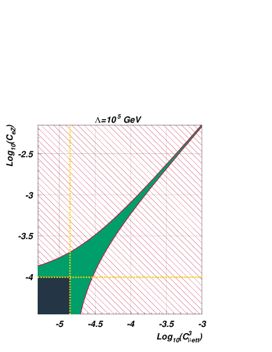
Figure 2: Correlations between $C_{eZ}^{\mu e}$ and $C^{(3)}_{\mu ett}$ (left) and $C^{(3)}_{\mu ett}$ and $C^{(1)}_{\mu ett}$ (right) at $\Lambda=10^{5}~{}{\rm GeV}$. The green area represents the allowed regions if both coefficients are allowed to deviate from zero.

A second limitation regarding the limits presented in Tables 4 and 5 is that they have been obtained assuming that only one coefficient at the time is non-zero. It is clear that such an assumption is rather unrealistic. A generic BSM model will usually introduce a large set of D-6 operators when heavy fields are integrated out. Allowing for more than one Wilson coefficient to be non zero, will introduce correlations that can lead to allowed regions that clearly violate the limits given in Tables 4 and 5. As an example we consider the case when simultaneously $C_{eZ}(\Lambda)$ and $C^{(3)}_{\mu ett}(\Lambda)$ are non-vanishing (left panel of Figure 2) as well as the case when simultaneously $C^{(3)}_{\mu ett}(\Lambda)$ and $C^{(1)}_{\mu ett}(\Lambda)$ are non-vanishing (right panel of Figure 2). The allowed region (green) is clearly much larger than the allowed regions if only one non-vanishing coupling at the time is allowed (indicated by the yellow dotted lines). In principle, arbitrarily large values for $C^{(3)}_{\mu ett}(\Lambda)$ are allowed, as long as $C_{eZ}(\Lambda)$ or $C^{(1)}_{\mu ett}(\Lambda)$ are tuned to provide an almost perfect cancellation. Such a fine-tuned choice of couplings is of course very unnatural and at some point is in conflict with the fixed-order constraint of $C_{eZ}$. Nevertheless, it has to be mentioned that the limits presented in this analysis are to be taken more as guidelines rather than strict limits. A more complete analysis with several observables would be required to disentangle the correlations and get strict limits on the various Wilson coefficients.

Finally, we recall that for $\lambda<m_{V}$ we have considered only the running of $C_{e\gamma}$ induced by the pure QED contributions. The effect of the running of $C_{e\gamma}$ from $\lambda=m_{\mu}$ to $\lambda=m_{V}$ is below 10% and we have checked that the impact of the terms with Yukawa couplings is completely negligible. Hence, the use of this approximation will affect the limits presented here by a few percent at most. The only possible exception to this is the limit on $C^{(3)}_{\mu ecc}$. As can be seen from Eq. (4.2), if $C^{(3)}_{\mu ecc}$ is much larger than $C_{e\gamma}$ the running of $C_{e\gamma}$ for $m_{c}<\lambda<m_{V}$ is modified noticeably. Such a situation can occur when considering the case $C^{(3)}_{\mu ecc}(\Lambda)\neq 0$ and all other $C_{i}(\Lambda)=0$, as done in obtaining the limit on $C^{(3)}_{\mu ecc}$. In particular, if $\Lambda$ is rather small, a very large $C^{(3)}_{\mu ecc}(\Lambda)$ is required to induce a sizable $C_{e\gamma}(m_{V})$. We have checked that, depending on the choice of $\Lambda$, the naive limits obtained by having only $C^{(3)}_{\mu ecc}(\Lambda)\neq 0$ can be modified by up to a factor two when taking into account its contribution to the RG evolution for $\lambda<m_{V}$. The effect will be much smaller for a more realistic scenario with several non-vanishing coefficients at the large scale $\Lambda$.

5 Conclusions

In this paper a complete one-loop analysis of the LFV decay $\mu\to e\gamma$ in the context of an EFT with D-6 operators has been presented. The main results are the limits on the (scale-dependent) Wilson coefficients at the large matching scale. These limits provide the most direct information on possible BSM models that can be obtained from the $\mu\to e\gamma$ decay in an EFT framework.

It is not surprising that the limit on ${\rm BR}(\mu^{+}\to e^{+}\gamma)$ results in a constraint on $C_{e\gamma}$, the Wilson coefficient of the operator $Q_{e\gamma}$ that induces a tree-level $\mu\to e\gamma$ transition. What is more remarkable is that constraints can be obtained also for a rather large number of further Wilson coefficients. These belong to operators that indirectly induce a LFV transition, either at one loop or through mixing under RG evolution. In this context it is important to note that the Wilson coefficients are scale dependent quantities and that in general operators mix under RG evolution. Thus, the presence at the large matching scale of any non-vanishing Wilson coefficient for an operator that mixes with $Q_{e\gamma}$ under RG evolution will induce a LFV transition $\mu\to e\gamma$ at the low scale.

It is clear that such an analysis can be applied to other processes as well. In particular, other LFV decays such as $\tau\to e\gamma$ or $\tau\to\mu\gamma$ lead immediately to similar constraints for the D-6 operators with other generation indices, as detailed in Appendix C. But in principle, any observable for which there are strong experimental constraints can be used. A combined analysis with many observables will also potentially allow to disentangle correlations between Wilson coefficients. Such correlations in the RG running result in unnatural allowed regions which are governed by large cancellations.

Depending on the process under consideration the inclusion of all D-6 operators, not only those listed in Tables 1 and 2 might be required. While this results in a more complicated system, such an analysis allows to combine consistently experimental results that have been obtained at completely different energy scales. In the absence of clear evidence for BSM physics at collider experiments, an extended EFT analysis providing constraints on many Wilson coefficients directly at the large scale can give useful clues in the search for a realistic BSM scenario and we consider this to be a very promising and useful strategy.

Appendix A D-6 effective $\mu-e-\gamma$ interaction at one-loop: the Feynman rule

In this appendix, the Feynman rule for the $\mu-e-\gamma$ interaction in the context of a D-6 ET is presented together with a complete treatment of the LFV wave-function renormalisation. Here and in Appendix B we keep the generation indices of the Wilson coefficients $C_{e\gamma}$, $C_{eZ}$ and $C_{e\varphi}$, but for notational simplicity drop the complex conjugate sign, i.e $(C_{e\gamma}^{\mu e})^{*}\to C_{e\gamma}^{\mu e}$.

In Eq. (A.1), the structure of the interaction is introduced in terms of the new scale $\Lambda$ and four effective coefficients related to the four possible contributions: vectorial left/right ($K_{VL}/K_{VR}$) and tensorial left/right ($K_{TL}/K_{TR}$). All momenta are considered to be incoming.

$$=\frac{1}{\Lambda^{2}}\left[\gamma^{\mu}\left(K_{VL}\,\omega_{L}+K_{VR}\,\omega_{R}\right)+\right.\left.i\sigma^{\mu\nu}\left(K_{TL}\,\omega_{L}+K_{TR}\,\omega_{R}\right)\left(p_{2}\right)_{\nu}\right].$$ (A.1)

The coefficients of Eq. (A.1) are connected to the one-loop wave-function renormalisation factors through

$$\frac{K_{VL}}{\Lambda^{2}} =-\frac{e}{2}\left(\frac{1}{2}\delta Z_{e\mu}^{L}+\frac{1}{2}\left(\delta Z_{e\mu}^{L}\right)^{\dagger}\right)-\frac{ev^{2}}{4c_{W}s_{W}\Lambda^{2}}\left(C_{\varphi l}^{(1)}+C_{\varphi l}^{(3)}\right)\frac{1}{2}\delta Z_{ZA},$$ (A.2)

$$\frac{K_{VR}}{\Lambda^{2}} =-\frac{e}{2}\left(\frac{1}{2}\delta Z_{e\mu}^{R}+\frac{1}{2}\left(\delta Z_{e\mu}^{R}\right)^{\dagger}\right)-\frac{ev^{2}}{4c_{W}s_{W}\Lambda^{2}}C_{\varphi e}\frac{1}{2}\delta Z_{ZA},$$ (A.3)

$$\frac{K_{TL}}{\Lambda^{2}} =-\frac{v}{\sqrt{2}\Lambda^{2}}C_{e\gamma}^{\mu e}\left(1+\frac{1}{2}\delta Z_{\mu\mu}^{L}+\frac{1}{2}\left(\delta Z_{ee}^{R}\right)^{\dagger}+\frac{1}{2}\delta Z_{AA}+\frac{\delta v}{v}\right)-\frac{v}{\sqrt{2}\Lambda^{2}}C_{eZ}^{\mu e}\frac{1}{2}\delta Z_{ZA},$$ (A.4)

$$\frac{K_{TR}}{\Lambda^{2}} =-\frac{v}{\sqrt{2}\Lambda^{2}}C_{e\gamma}^{e\mu}\left(1+\frac{1}{2}\delta Z_{\mu\mu}^{R}+\frac{1}{2}\left(\delta Z_{ee}^{L}\right)^{\dagger}+\frac{1}{2}\delta Z_{AA}+\frac{\delta v}{v}\right)-\frac{v}{\sqrt{2}\Lambda^{2}}C_{eZ}^{e\mu}\frac{1}{2}\delta Z_{ZA}.$$ (A.5)

Several elements of Eqns. (A.2)-(A.5) do not belong to the SM framework: the effective coefficients $C_{e\gamma}$, $C_{eZ}$, $C_{\varphi l}^{(1)}$, $C_{\varphi l}^{(3)}$ and $C_{\varphi e}$, plus the off-diagonal leptonic wave-function renormalisation. For further information, a complete treatment of LFV wave-function renormalisation in the on-shell scheme is given.

Making use of standard techniques (e.g., see Denner (1993)), the off-diagonal leptonic self-energy (for conventions used see Figure 3) was calculated. Then, the renormalisation conditions in the on-shell scheme have been applied to obtain the various contributions to the off-diagonal wave-function renormalisation.

Figure 3: Conventions used for the one-particle irreducible two-point functions.

The tensorial structure that corresponds to such transition consists of four possible coefficients:

$$\Gamma^{f}_{ij}(p)=i\delta_{ij}(\not{p}-m_{i})+i\left[\not{p}\,\omega_{L}\,\Sigma^{f,L}_{ij}(p^{2})+\not{p}\,\omega_{R}\,\Sigma^{f,R}_{ij}(p^{2})+\omega_{L}\,\Sigma^{f,l}_{ij}(p^{2})+\omega_{R}\,\Sigma^{f,r}_{ij}(p^{2})\right].$$ (A.6)

By applying the standard on-shell renormalisation conditions

$$\left.{\rm Re}\!\left[\Gamma^{f}_{ij}(p)\right]u_{j}(p)\right|_{p^{2}=m_{j}^{2}} =0,$$ (A.7)

$$\bar{u}_{i}(p){\rm Re}\!\left[\Gamma^{f}_{ij}(p)\right]_{p^{2}=m_{i}^{2}} =0,$$ (A.8)

one finds the off-diagonal wave-function renormalisation that is required in Eqs. (A.2) and (A.3) to determine the coefficients $K_{VL}$ and $K_{VR}$ of Eq. (A.1):

$$\delta Z_{ij}^{L} =\frac{4}{m^{2}_{i}-m^{2}_{j}}\left(m_{j}^{2}\Sigma^{f,L}_{ij}(m_{j}^{2})+m_{i}m_{j}\Sigma^{f,R}_{ij}(m_{j}^{2})+m_{j}\Sigma^{f,r}_{ij}(m_{j}^{2})+m_{i}\Sigma^{f,l}_{ij}(m_{j}^{2})\right),$$ (A.9)

$$\delta Z_{ij}^{R} =\frac{4}{m^{2}_{i}-m^{2}_{j}}\left(m_{j}^{2}\Sigma^{f,R}_{ij}(m_{j}^{2})+m_{i}m_{j}\Sigma^{f,L}_{ij}(m_{j}^{2})+m_{j}\Sigma^{f,l}_{ij}(m_{j}^{2})+m_{i}\Sigma^{f,r}_{ij}(m_{j}^{2})\right).$$ (A.10)

The explicit result for the four coefficients of Eq. (A.6) are as follows:

$$\quad\Sigma^{f,L}_{e\mu}(p^{2})\Lambda^{2}$$

$$=A_{0}\left[m_{e}^{2}\right]\left(-\frac{m_{e}}{64\pi^{2}}C_{\varphi l}^{(1)}-\frac{m_{e}}{64\pi^{2}}C_{\varphi l}^{(3)}-\frac{3m_{Z}s_{W}^{2}}{16\sqrt{2}\pi^{2}}C_{eZ}^{\mu e}+\frac{3m_{Z}(2s_{W}c_{W})}{32\sqrt{2}\pi^{2}}C_{e\gamma}^{\mu e}\right)$$

$$+A_{0}\left[m_{\mu}^{2}\right]\left(\frac{m_{\mu}}{64\pi^{2}}C_{\varphi e}+\frac{3m_{Z}(c_{W}^{2}-s_{W}^{2})}{32\sqrt{2}\pi^{2}}C_{eZ}^{\mu e}+\frac{3m_{Z}(2s_{W}c_{W})}{32\sqrt{2}\pi^{2}}C_{e\gamma}^{\mu e}\right)$$

$$+A_{0}\left[m_{W}^{2}\right]\left(\frac{3m_{Z}c_{W}^{2}}{16\sqrt{2}\pi^{2}}C_{eZ}^{\mu e}+\frac{3m_{Z}(2s_{W}c_{W})}{32\sqrt{2}\pi^{2}}C_{e\gamma}^{\mu e}\right)$$

$$+A_{0}\left[\xi_{W}m_{W}^{2}\right]\left(-\frac{m_{e}}{32\pi^{2}}C_{\varphi l}^{(3)}-\frac{m_{Z}(2s_{W}c_{W})}{32\sqrt{2}e\pi^{2}}C_{e\varphi}^{\mu e}\right)$$

$$+A_{0}\left[m_{Z}^{2}\right]\left(\frac{3m_{Z}(-1+2(c_{W}^{2}-s_{W}^{2}))}{32\sqrt{2}\pi^{2}}C_{eZ}^{\mu e}\right)$$

$$+A_{0}\left[\xi_{Z}m_{Z}^{2}\right]\left(\frac{m_{\mu}}{64\pi^{2}}C_{\varphi e}-\frac{m_{e}}{64\pi^{2}}C_{\varphi l}^{(1)}-\frac{m_{e}}{64\pi^{2}}C_{\varphi l}^{(3)}-\frac{m_{Z}c_{W}s_{W}}{32\sqrt{2}e\pi^{2}}C_{e\varphi}^{\mu e}\right)$$

$$+A_{0}\left[m_{H}^{2}\right]\left(-\frac{3m_{Z}c_{W}s_{W}}{32\sqrt{2}e\pi^{2}}C_{e\varphi}^{\mu e}\right)$$

$$+B_{0}\left[p^{2},m_{Z}^{2},m_{e}^{2}\right]\left(\frac{3m_{e}m_{Z}^{2}s_{W}^{2}}{16\pi^{2}}C_{\varphi l}^{(1)}+\frac{3m_{e}m_{Z}^{2}s_{W}^{2}}{16\pi^{2}}C_{\varphi l}^{(3)}-\frac{3m_{Z}\left(m_{e}^{2}+m_{Z}^{2}-p^{2}\right)s_{W}^{2}}{16\sqrt{2}\pi^{2}}C_{eZ}^{\mu e}\right)$$

$$+B_{0}\left[p^{2},\xi_{Z}m_{Z}^{2},m_{e}^{2}\right]\left(\frac{m_{e}\left(-m_{e}^{2}+\xi_{Z}m_{Z}^{2}+p^{2}-2\xi_{Z}m_{Z}^{2}(c_{W}^{2}-s_{W}^{2})\right)}{64\pi^{2}}(C_{\varphi l}^{(1)}+C_{\varphi l}^{(3)})\right)$$

$$+B_{0}\left[p^{2},m_{Z}^{2},m_{\mu}^{2}\right]\left(-\frac{3m_{\mu}m_{Z}^{2}(c_{W}^{2}-s_{W}^{2})}{32\pi^{2}}C_{\varphi e}+\frac{3m_{Z}\left(m_{\mu}^{2}+m_{Z}^{2}-p^{2}\right)(c_{W}^{2}-s_{W}^{2})}{32\sqrt{2}\pi^{2}}C_{eZ}^{\mu e}\right)$$

$$+B_{0}\left[p^{2},\xi_{Z}m_{Z}^{2},m_{\mu}^{2}\right]\left(\frac{m_{\mu}\left(m_{\mu}^{2}+\xi_{Z}m_{Z}^{2}-p^{2}-2\xi_{Z}m_{Z}^{2}(c_{W}^{2}-s_{W}^{2})\right)}{64\pi^{2}}C_{\varphi e}\right)$$

$$+B_{0}\left[p^{2},m_{W}^{2},0\right]\left(\frac{3m_{Z}\left(m_{W}^{2}-p^{2}\right)c_{W}^{2}}{16\sqrt{2}\pi^{2}}C_{eZ}^{\mu e}+\frac{3m_{Z}\left(m_{W}^{2}-p^{2}\right)(2s_{W}c_{W})}{32\sqrt{2}\pi^{2}}C_{e\gamma}^{\mu e}\right)$$

$$+B_{0}\left[p^{2},\xi_{W}m_{W}^{2},0\right]\left(\frac{m_{e}\left(-\xi_{W}m_{W}^{2}+p^{2}\right)}{32\pi^{2}}C_{\varphi l}^{(3)}\right)$$

$$+B_{0}\left[p^{2},m_{H}^{2},m_{e}^{2}\right]\left(-\frac{m_{e}^{2}m_{Z}(2s_{W}c_{W})}{32\sqrt{2}e\pi^{2}}C_{e\varphi}^{\mu e}\right)$$

$$+B_{0}\left[p^{2},m_{H}^{2},m_{\mu}^{2}\right]\left(-\frac{m_{\mu}^{2}m_{Z}(2s_{W}c_{W})}{32\sqrt{2}e\pi^{2}}C_{e\varphi}^{\mu e}\right)$$

$$+B_{0}\left[p^{2},0,m_{e}^{2}\right]\left(\frac{3m_{Z}\left(m_{e}^{2}-p^{2}\right)(2s_{W}c_{W})}{32\sqrt{2}\pi^{2}}C_{e\gamma}^{\mu e}\right)$$

$$+B_{0}\left[p^{2},0,m_{\mu}^{2}\right]\left(\frac{3m_{Z}\left(m_{\mu}^{2}-p^{2}\right)(2s_{W}c_{W})}{32\sqrt{2}\pi^{2}}C_{e\gamma}^{\mu e}\right)$$

$$+\frac{m_{\mu}m_{Z}^{2}(c_{W}^{2}-s_{W}^{2})}{16\pi^{2}}C_{\varphi e}-\frac{m_{e}m_{Z}^{2}s_{W}^{2}}{8\pi^{2}}C_{\varphi l}^{(1)}-\frac{m_{e}m_{Z}^{2}s_{W}^{2}}{8\pi^{2}}C_{\varphi l}^{(3)}$$

$$-\frac{m_{Z}}{16\sqrt{2}\pi^{2}}\left(-2\left(m_{e}^{2}-m_{W}^{2}+m_{Z}^{2}\right)+\left(2m_{e}^{2}+2m_{\mu}^{2}+2m_{W}^{2}+4m_{Z}^{2}-3p^{2}\right)(c_{W}^{2}-s_{W}^{2})\right)C_{eZ}^{\mu e}$$

$$-\frac{m_{Z}\left(2m_{e}^{2}+2m_{\mu}^{2}+2m_{W}^{2}-3p^{2}\right)c_{W}s_{W}}{8\sqrt{2}\pi^{2}}C_{e\gamma}^{\mu e}.$$ (A.11)

$$\quad\Sigma^{f,R}_{e\mu}(p^{2})=\Sigma^{f,L}_{e\mu}(p^{2})\big{|}_{\mu\leftrightarrow e}$$ (A.12)

$$\quad\Sigma^{f,l}_{e\mu}(p^{2})\Lambda^{2}$$

$$=A_{0}\left[m_{e}^{2}\right]\left(-\frac{\left(m_{e}^{2}+2m_{Z}^{2}(c_{W}^{2}-s_{W}^{2})\right)}{64p^{2}\pi^{2}}(C_{\varphi l}^{(1)}+C_{\varphi l}^{(3)})+\frac{m_{e}m_{Z}c_{W}s_{W}}{32\sqrt{2}ep^{2}\pi^{2}}C_{e\varphi}^{\mu e}\right.$$

$$+\left.\frac{3m_{e}m_{Z}(c_{W}^{2}-s_{W}^{2})}{32\sqrt{2}p^{2}\pi^{2}}C_{eZ}^{\mu e}+\frac{3m_{e}m_{Z}(2s_{W}c_{W})}{32\sqrt{2}p^{2}\pi^{2}}C_{e\gamma}^{\mu e}\right)$$

$$+A_{0}\left[m_{\mu}^{2}\right]\left(-\frac{\left(m_{\mu}^{2}+2m_{Z}^{2}(c_{W}^{2}-s_{W}^{2})\right)}{64p^{2}\pi^{2}}(C_{\varphi l}^{(1)}+C_{\varphi l}^{(3)})+\frac{m_{\mu}m_{Z}(2s_{W}c_{W})}{64\sqrt{2}ep^{2}\pi^{2}}C_{e\varphi}^{e\mu}\right.$$

$$+\left.\frac{3m_{\mu}m_{Z}(c_{W}^{2}-s_{W}^{2})}{32\sqrt{2}p^{2}\pi^{2}}C_{eZ}^{e\mu}+\frac{3m_{\mu}m_{Z}(2s_{W}c_{W})}{32\sqrt{2}p^{2}\pi^{2}}C_{e\gamma}^{e\mu}\right)$$

$$+A_{0}\left[m_{W}^{2}\right]\left(\frac{m_{Z}^{2}\left(2m_{W}^{2}-p^{2}\right)c_{W}^{2}}{16m_{W}^{2}p^{2}\pi^{2}}C_{\varphi l}^{(3)}\right)$$

$$+A_{0}\left[\xi_{W}m_{W}^{2}\right]\left(\frac{m_{Z}^{2}c_{W}^{2}}{16m_{W}^{2}\pi^{2}}C_{\varphi l}^{(3)}\right)$$

$$+A_{0}\left[m_{Z}^{2}\right]\left(\frac{\left(m_{e}^{2}+m_{\mu}^{2}+4m_{Z}^{2}-2p^{2}\right)(c_{W}^{2}-s_{W}^{2})}{64p^{2}\pi^{2}}(C_{\varphi l}^{(1)}+C_{\varphi l}^{(3)})\right.$$

$$-\left.\frac{3m_{\mu}m_{Z}(c_{W}^{2}-s_{W}^{2})}{32\sqrt{2}p^{2}\pi^{2}}C_{eZ}^{e\mu}-\frac{3m_{e}m_{Z}(c_{W}^{2}-s_{W}^{2})}{32\sqrt{2}p^{2}\pi^{2}}C_{eZ}^{\mu e}\right)$$

$$+A_{0}\left[\xi_{Z}m_{Z}^{2}\right]\left(\frac{\left(m_{e}^{2}+m_{\mu}^{2}-\left(m_{e}^{2}+m_{\mu}^{2}-2p^{2}\right)(c_{W}^{2}-s_{W}^{2})\right)}{64p^{2}\pi^{2}}(C_{\varphi l}^{(1)}+C_{\varphi l}^{(3)})\right)$$

$$+A_{0}\left[m_{H}^{2}\right]\left(-\frac{m_{\mu}m_{Z}c_{W}s_{W}}{32\sqrt{2}ep^{2}\pi^{2}}C_{e\varphi}^{e\mu}-\frac{m_{e}m_{Z}c_{W}s_{W}}{32\sqrt{2}ep^{2}\pi^{2}}C_{e\varphi}^{\mu e}\right)$$

$$+B_{0}\left[p^{2},m_{Z}^{2},m_{e}^{2}\right]\left(\frac{\left(m_{e}^{4}-2m_{Z}^{4}+m_{e}^{2}\left(m_{Z}^{2}-2p^{2}\right)+m_{Z}^{2}p^{2}+p^{4}\right)(c_{W}^{2}-s_{W}^{2})}{64p^{2}\pi^{2}}(C_{\varphi l}^{(1)}+C_{\varphi l}^{(3)})\right.$$

$$+\left.\frac{3m_{e}m_{Z}\left(-m_{e}^{2}+m_{Z}^{2}+p^{2}\right)(c_{W}^{2}-s_{W}^{2})}{32\sqrt{2}p^{2}\pi^{2}}C_{eZ}^{\mu e}\right)$$

$$+B_{0}\left[p^{2},\xi_{Z}m_{Z}^{2},m_{e}^{2}\right]\left(\frac{1}{64p^{2}\pi^{2}}\left(m_{e}^{2}\left(m_{e}^{2}-\xi_{Z}m_{Z}^{2}-p^{2}\right)+\left(-m_{e}^{4}+\left(\xi_{Z}m_{Z}^{2}-p^{2}\right)p^{2}\right.\right.\right.$$

$$+\left.\left.\left.m_{e}^{2}\left(\xi_{Z}m_{Z}^{2}+2p^{2}\right)\right)(c_{W}^{2}-s_{W}^{2})\right)(C_{\varphi l}^{(1)}+C_{\varphi l}^{(3)})\right)$$

$$+B_{0}\left[p^{2},m_{Z}^{2},m_{\mu}^{2}\right]\left(\frac{\left(m_{\mu}^{4}-2m_{Z}^{4}+m_{\mu}^{2}\left(m_{Z}^{2}-2p^{2}\right)+m_{Z}^{2}p^{2}+p^{4}\right)(c_{W}^{2}-s_{W}^{2})}{64p^{2}\pi^{2}}(C_{\varphi l}^{(1)}+C_{\varphi l}^{(3)})\right.$$

$$+\left.\frac{3m_{\mu}m_{Z}\left(-m_{\mu}^{2}+m_{Z}^{2}+p^{2}\right)(c_{W}^{2}-s_{W}^{2})}{32\sqrt{2}p^{2}\pi^{2}}C_{eZ}^{e\mu}\right)$$

$$+B_{0}\left[p^{2},\xi_{Z}m_{Z}^{2},m_{\mu}^{2}\right]\left(\frac{1}{64p^{2}\pi^{2}}\left(m_{\mu}^{2}\left(m_{\mu}^{2}-\xi_{Z}m_{Z}^{2}-p^{2}\right)+\left(-m_{\mu}^{4}+\left(\xi_{Z}m_{Z}^{2}-p^{2}\right)p^{2}\right.\right.\right.$$

$$+\left.\left.\left.m_{\mu}^{2}\left(\xi_{Z}m_{Z}^{2}+2p^{2}\right)\right)(c_{W}^{2}-s_{W}^{2})\right)(C_{\varphi l}^{(1)}+C_{\varphi l}^{(3)})\right)$$

$$+B_{0}\left[p^{2},m_{W}^{2},0\right]\left(-\frac{m_{Z}^{2}\left(2m_{W}^{4}-m_{W}^{2}p^{2}-p^{4}\right)c_{W}^{2}}{16m_{W}^{2}p^{2}\pi^{2}}C_{\varphi l}^{(3)}\right)$$

$$+B_{0}\left[p^{2},\xi_{W}m_{W}^{2},0\right]\left(\frac{m_{Z}^{2}\left(\xi_{W}m_{W}^{2}-p^{2}\right)c_{W}^{2}}{16m_{W}^{2}\pi^{2}}C_{\varphi l}^{(3)}\right)$$

$$+B_{0}\left[p^{2},m_{H}^{2},m_{e}^{2}\right]\left(-\frac{m_{e}m_{Z}\left(m_{e}^{2}-m_{H}^{2}+p^{2}\right)(2s_{W}c_{W})}{64\sqrt{2}ep^{2}\pi^{2}}C_{e\varphi}^{\mu e}\right)$$

$$+B_{0}\left[p^{2},m_{H}^{2},m_{\mu}^{2}\right]\left(-\frac{m_{\mu}m_{Z}\left(-m_{H}^{2}+m_{\mu}^{2}+p^{2}\right)(2s_{W}c_{W})}{64\sqrt{2}ep^{2}\pi^{2}}C_{e\varphi}^{e\mu}\right)$$

$$+B_{0}\left[p^{2},0,m_{e}^{2}\right]\left(-\frac{3m_{e}m_{Z}\left(m_{e}^{2}-p^{2}\right)(2s_{W}c_{W})}{32\sqrt{2}p^{2}\pi^{2}}C_{e\gamma}^{\mu e}\right)$$

$$+B_{0}\left[p^{2},0,m_{\mu}^{2}\right]\left(-\frac{3m_{\mu}m_{Z}\left(m_{\mu}^{2}-p^{2}\right)(2s_{W}c_{W})}{32\sqrt{2}p^{2}\pi^{2}}C_{e\gamma}^{e\mu}\right)$$

$$-\frac{m_{Z}^{2}(c_{W}^{2}-s_{W}^{2})}{16\pi^{2}}C_{\varphi l}^{(1)}-\frac{m_{Z}^{2}(1+2(c_{W}^{2}-s_{W}^{2}))}{16\pi^{2}}C_{\varphi l}^{(3)}-\frac{m_{\mu}m_{Z}(c_{W}^{2}-s_{W}^{2})}{16\sqrt{2}\pi^{2}}C_{eZ}^{e\mu}$$

$$-\frac{m_{e}m_{Z}(c_{W}^{2}-s_{W}^{2})}{16\sqrt{2}\pi^{2}}C_{eZ}^{\mu e}-\frac{m_{\mu}m_{Z}c_{W}s_{W}}{8\sqrt{2}\pi^{2}}C_{e\gamma}^{e\mu}-\frac{m_{e}m_{Z}c_{W}s_{W}}{8\sqrt{2}\pi^{2}}C_{e\gamma}^{\mu e}.$$ (A.13)

$$\quad\Sigma^{f,r}_{e\mu}(p^{2})\Lambda^{2}$$

$$=A_{0}\left[m_{e}^{2}\right]\left(\frac{\left(m_{e}^{2}+2m_{Z}^{2}-2m_{Z}^{2}(c_{W}^{2}-s_{W}^{2})\right)}{64p^{2}\pi^{2}}C_{\varphi e}+\frac{m_{e}m_{Z}c_{W}s_{W}}{32\sqrt{2}ep^{2}\pi^{2}}C_{e\varphi}^{e\mu}\right.$$

$$-\left.\frac{3m_{e}m_{Z}s_{W}^{2}}{16\sqrt{2}p^{2}\pi^{2}}C_{eZ}^{e\mu}+\frac{3m_{e}m_{Z}(2s_{W}c_{W})}{32\sqrt{2}p^{2}\pi^{2}}C_{e\gamma}^{e\mu}\right)$$

$$+A_{0}\left[m_{\mu}^{2}\right]\left(\frac{\left(m_{\mu}^{2}+2m_{Z}^{2}-2m_{Z}^{2}(c_{W}^{2}-s_{W}^{2})\right)}{64p^{2}\pi^{2}}C_{\varphi e}+\frac{m_{\mu}m_{Z}(2s_{W}c_{W})}{64\sqrt{2}ep^{2}\pi^{2}}C_{e\varphi}^{\mu e}\right.$$

$$-\left.\frac{3m_{\mu}m_{Z}s_{W}^{2}}{16\sqrt{2}p^{2}\pi^{2}}C_{eZ}^{\mu e}+\frac{3m_{\mu}m_{Z}(2s_{W}c_{W})}{32\sqrt{2}p^{2}\pi^{2}}C_{e\gamma}^{\mu e}\right)$$

$$+A_{0}\left[m_{Z}^{2}\right]\left(-\frac{\left(m_{e}^{2}+m_{\mu}^{2}+4m_{Z}^{2}-2p^{2}\right)s_{W}^{2}}{32p^{2}\pi^{2}}C_{\varphi e}+\frac{3m_{e}m_{Z}s_{W}^{2}}{16\sqrt{2}p^{2}\pi^{2}}C_{eZ}^{e\mu}+\frac{3m_{\mu}m_{Z}s_{W}^{2}}{16\sqrt{2}p^{2}\pi^{2}}C_{eZ}^{\mu e}\right)$$

$$+A_{0}\left[\xi_{Z}m_{Z}^{2}\right]\left(-\frac{\left(2p^{2}+\left(m_{e}^{2}+m_{\mu}^{2}-2p^{2}\right)(c_{W}^{2}-s_{W}^{2})\right)}{64p^{2}\pi^{2}}C_{\varphi e}\right)$$

$$+A_{0}\left[m_{H}^{2}\right]\left(-\frac{m_{e}m_{Z}c_{W}s_{W}}{32\sqrt{2}ep^{2}\pi^{2}}C_{e\varphi}^{e\mu}-\frac{m_{\mu}m_{Z}c_{W}s_{W}}{32\sqrt{2}ep^{2}\pi^{2}}C_{e\varphi}^{\mu e}\right)$$

$$+B_{0}\left[p^{2},m_{Z}^{2},m_{e}^{2}\right]\left(-\frac{\left(m_{e}^{4}-2m_{Z}^{4}+m_{e}^{2}\left(m_{Z}^{2}-2p^{2}\right)+m_{Z}^{2}p^{2}+p^{4}\right)s_{W}^{2}}{32p^{2}\pi^{2}}C_{\varphi e}\right.$$

$$-\left.\frac{3m_{e}m_{Z}\left(-m_{e}^{2}+m_{Z}^{2}+p^{2}\right)s_{W}^{2}}{16\sqrt{2}p^{2}\pi^{2}}C_{eZ}^{e\mu}\right)$$

$$+B_{0}\left[p^{2},\xi_{Z}m_{Z}^{2},m_{e}^{2}\right]\left(\frac{1}{64p^{2}\pi^{2}}\left(p^{2}\left(-m_{e}^{2}-\xi_{Z}m_{Z}^{2}+p^{2}\right)+\left(-m_{e}^{4}+\left(\xi_{Z}m_{Z}^{2}-p^{2}\right)p^{2}\right.\right.\right.$$

$$+\left.\left.\left.m_{e}^{2}\left(\xi_{Z}m_{Z}^{2}+2p^{2}\right)\right)(c_{W}^{2}-s_{W}^{2})\right)C_{\varphi e}\right)$$

$$+B_{0}\left[p^{2},m_{Z}^{2},m_{\mu}^{2}\right]\left(-\frac{\left(m_{\mu}^{4}-2m_{Z}^{4}+m_{\mu}^{2}\left(m_{Z}^{2}-2p^{2}\right)+m_{Z}^{2}p^{2}+p^{4}\right)s_{W}^{2}}{32p^{2}\pi^{2}}C_{\varphi e}\right.$$

$$-\left.\frac{3m_{\mu}m_{Z}\left(-m_{\mu}^{2}+m_{Z}^{2}+p^{2}\right)s_{W}^{2}}{16\sqrt{2}p^{2}\pi^{2}}C_{eZ}^{\mu e}\right)$$

$$+B_{0}\left[p^{2},\xi_{Z}m_{Z}^{2},m_{\mu}^{2}\right]\left(\frac{1}{64p^{2}\pi^{2}}\left(p^{2}\left(-m_{\mu}^{2}-\xi_{Z}m_{Z}^{2}+p^{2}\right)+\left(-m_{\mu}^{4}+\left(\xi_{Z}m_{Z}^{2}-p^{2}\right)p^{2}\right.\right.\right.$$

$$+\left.\left.\left.m_{\mu}^{2}\left(\xi_{Z}m_{Z}^{2}+2p^{2}\right)\right)(c_{W}^{2}-s_{W}^{2})\right)C_{\varphi e}\right)$$

$$+B_{0}\left[p^{2},m_{H}^{2},m_{e}^{2}\right]\left(-\frac{m_{e}m_{Z}\left(m_{e}^{2}-m_{H}^{2}+p^{2}\right)(2s_{W}c_{W})}{64\sqrt{2}ep^{2}\pi^{2}}C_{e\varphi}^{e\mu}\right)$$

$$+B_{0}\left[p^{2},m_{H}^{2},m_{\mu}^{2}\right]\left(-\frac{m_{\mu}m_{Z}\left(-m_{H}^{2}+m_{\mu}^{2}+p^{2}\right)(2s_{W}c_{W})}{64\sqrt{2}ep^{2}\pi^{2}}C_{e\varphi}^{\mu e}\right)$$

$$+B_{0}\left[p^{2},0,m_{e}^{2}\right]\left(-\frac{3m_{e}m_{Z}\left(m_{e}^{2}-p^{2}\right)(2s_{W}c_{W})}{32\sqrt{2}p^{2}\pi^{2}}C_{e\gamma}^{e\mu}\right)$$

$$+B_{0}\left[p^{2},0,m_{\mu}^{2}\right]\left(-\frac{3m_{\mu}m_{Z}\left(m_{\mu}^{2}-p^{2}\right)(2s_{W}c_{W})}{32\sqrt{2}p^{2}\pi^{2}}C_{e\gamma}^{\mu e}\right)$$

$$+\frac{m_{Z}^{2}s_{W}^{2}}{8\pi^{2}}C_{\varphi e}-\frac{m_{e}m_{Z}c_{W}s_{W}}{8\sqrt{2}\pi^{2}}C_{e\gamma}^{e\mu}-\frac{m_{\mu}m_{Z}c_{W}s_{W}}{8\sqrt{2}\pi^{2}}C_{e\gamma}^{\mu e}$$

$$+\frac{m_{e}m_{Z}s_{W}^{2}}{8\sqrt{2}\pi^{2}}C_{eZ}^{e\mu}+\frac{m_{\mu}m_{Z}s_{W}^{2}}{8\sqrt{2}\pi^{2}}C_{eZ}^{\mu e}.$$ (A.14)

The explicit results for the four coefficients of the off-diagonal one-particle irreducible two-point function for leptons are sufficient to obtain the wave-function renormalisation factors Eqs. (A.9) and (A.10).

Finally, for completeness we list the required SM expressions for the renormalisation. The expression

$$\delta Z_{ZA}=\frac{\left(c_{W}e^{2}\left(2\left(-1+\xi_{W}^{2}\right)m_{W}^{2}-(-9+\xi_{W})A_{0}\left[m_{W}^{2}\right]-(5+3\xi_{W})A_{0}\left[\xi_{W}m_{W}^{2}\right]\right)\right)}{\left(48(-1+\xi_{W})m_{W}^{2}\pi^{2}s_{W}\right)}$$ (A.15)

is needed in Eqs.(A.2)-(A.5) and the following expressions in the $\overline{\rm MS}$ scheme are required for the computation of the anomalous dimensions analysed in Section 4.2:

$$\widehat{\Delta}^{-1}\delta Z_{AA} =-\frac{e^{2}(20+3\xi_{W})}{48\pi^{2}},$$ (A.16)

$$\widehat{\Delta}^{-1}\delta Z_{ZZ} =-\frac{e^{2}\left(-1+2s_{W}^{2}+40s_{W}^{4}+6c_{W}^{4}\xi_{W}\right)}{96\pi^{2}c_{W}^{2}s_{W}^{2}},$$ (A.17)

$$\widehat{\Delta}^{-1}\delta Z_{e} =-\frac{1}{2}\delta Z_{AA}+\frac{s_{W}}{c_{W}}\frac{1}{2}\delta Z_{ZA}=\frac{11e^{2}}{96\pi^{2}},$$ (A.18)

$$\widehat{\Delta}^{-1}\delta m_{W}^{2} =+\frac{e^{2}m_{W}^{2}}{32\pi^{2}s_{W}^{2}}\xi_{W}+\frac{e^{2}m_{Z}^{2}}{64\pi^{2}s_{W}^{2}}\xi_{Z}$$

$$-\frac{e^{2}\left(6\left(N_{c}\sum_{q}m_{q}^{2}+\sum_{l}m_{l}^{2}\right)+11m_{Z}^{2}-20m_{Z}^{2}s_{W}^{2}\right)}{192\pi^{2}s_{W}^{2}},$$ (A.19)

$$\widehat{\Delta}^{-1}\delta m_{Z}^{2} =+\frac{e^{2}m_{W}^{2}}{32\pi^{2}c_{W}^{2}s_{W}^{2}}\xi_{W}+\frac{e^{2}m_{Z}^{2}}{64\pi^{2}c_{W}^{2}s_{W}^{2}}\xi_{Z}$$

$$-\frac{e^{2}\left(6\left(N_{c}\sum_{q}m_{q}^{2}+\sum_{l}m_{l}^{2}\right)+11m_{Z}^{2}-58m_{Z}^{2}s_{W}^{2}-44m_{Z}^{2}s_{W}^{4}\right)}{192\pi^{2}c_{W}^{2}s_{W}^{2}},$$ (A.20)

$$\widehat{\Delta}^{-1}\frac{\delta v}{v} =\left(1-\frac{1}{2s_{W}^{2}}\right)\frac{\delta m_{W}^{2}}{m_{W}^{2}}+\frac{c_{W}^{2}}{2s_{W}^{2}}\frac{\delta m_{Z}^{2}}{m_{Z}^{2}}-\delta Z_{e}=\frac{e^{2}}{64\pi^{2}s_{W}^{2}}\xi_{W}$$

$$+\frac{e^{2}}{128\pi^{2}c_{W}^{2}s_{W}^{2}}\xi_{Z}-\frac{e^{2}\left(2\left(N_{c}\sum_{q}m_{q}^{2}+\sum_{l}m_{l}^{2}\right)-9m_{Z}^{2}+6m_{Z}^{2}s_{W}^{2}\right)}{128m_{Z}^{2}\pi^{2}c_{W}^{2}s_{W}^{2}},$$ (A.21)

$$\widehat{\Delta}^{-1}\delta Z_{ll}^{R} =-\frac{e^{2}\left(m_{l}^{2}+2m_{Z}^{2}s_{W}^{2}\left(c_{W}^{2}\xi_{\gamma}+s_{W}^{2}\xi_{Z}\right)\right)}{32m_{Z}^{2}\pi^{2}c_{W}^{2}s_{W}^{2}},$$ (A.22)

$$\widehat{\Delta}^{-1}\delta Z_{ll}^{L} =-\frac{e^{2}\left(m_{l}^{2}+m_{Z}^{2}\left(4c_{W}^{2}s_{W}^{2}\xi_{\gamma}+2c_{W}^{2}\xi_{W}+\left(1-2s_{W}^{2}\right)^{2}\xi_{Z}\right)\right)}{64m_{Z}^{2}\pi^{2}c_{W}^{2}s_{W}^{2}},$$ (A.23)

$$\widehat{\Delta}^{-1}\delta Z_{tt}^{R} =-\frac{e^{2}m_{t}^{2}}{32m_{Z}^{2}\pi^{2}s_{W}^{2}c_{W}^{2}}-\frac{e^{2}}{36\pi^{2}}\xi_{\gamma}-\frac{e^{2}s_{W}^{2}}{36\pi^{2}c_{W}^{2}}\xi_{Z}-\frac{g_{S}^{2}}{12\pi^{2}}\xi_{G},$$ (A.24)

$$\widehat{\Delta}^{-1}\delta Z_{tt}^{L} =-\frac{e^{2}\left(m_{t}^{2}+\sum_{d}\left|V_{d3}\right|^{2}m_{d}^{2}\right)}{64m_{Z}^{2}\pi^{2}s_{W}^{2}c_{W}^{2}}-\frac{e^{2}}{36\pi^{2}}\xi_{\gamma}-\frac{e^{2}}{32\pi^{2}s_{W}^{2}}\xi_{W}$$

$$-\frac{e^{2}\left(3-4s_{W}^{2}\right)^{2}}{576\pi^{2}s_{W}^{2}c_{W}^{2}}\xi_{Z}-\frac{g_{S}^{2}}{12\pi^{2}}\xi_{G},$$ (A.25)

$$\widehat{\Delta}^{-1}\delta Z_{ct}^{R} =-\frac{e^{2}m_{c}^{2}m_{t}^{2}\sum_{d}V_{3d}V_{2d}^{\dagger}}{32m_{Z}^{2}\pi^{2}s_{W}^{2}c_{W}^{2}}=0,$$ (A.26)

$$\widehat{\Delta}^{-1}\delta Z_{ct}^{L} =-\frac{e^{2}\sum_{d}V_{3d}V_{2d}^{\dagger}m_{d}^{2}}{32m_{Z}^{2}\pi^{2}s_{W}^{2}c_{W}^{2}}-\frac{e^{2}\sum_{d}V_{3d}V_{2d}^{\dagger}}{16\pi^{2}s_{W}^{2}}\xi_{W}=-\frac{e^{2}\sum_{d}V_{3d}V_{2d}^{\dagger}m_{d}^{2}}{32m_{Z}^{2}\pi^{2}s_{W}^{2}c_{W}^{2}},$$ (A.27)

where

$$\widehat{\Delta}=\left[\frac{2}{4-D}-\gamma_{E}+\log{4\pi}\right],$$ (A.28)

with $D$ being the dimensional-regularisation parameter and $\gamma_{E}$ the Euler-Mascheroni constant. All the above equations have been cross checked against Denner (1993) and Bardin and Passarino (1999).

Appendix B Explicit one-loop result for $\mu-e-\gamma$

In this appendix, the complete result for the unrenormalised coefficients $\bar{C}_{TL}$ and $\bar{C}_{TR}$ of the $\mu^{-}\to e^{-}\gamma$ decay in the EFT is given. After renormalisation, the formulae were further expanded around $m_{l}\ll m_{V}$ to obtain the results in Table 3; then the public package LoopTools 2.10 Hahn and Perez-Victoria (1999) was used to check the numerical stability of the aforementioned expansion. The result is presented in terms of Passarino-Veltman functions Passarino and Veltman (1979), following the convention described in Denner (1993). Writing the coefficients as

$$\bar{C}_{TL} =C_{TL}^{(A_{0})}+C_{TL}^{(B_{0})}+C_{TL}^{(C_{0})}+C_{TL}^{(c)},$$ (B.1)

$$\bar{C}_{TR} =\bar{C}_{TL}\big{|}_{e\leftrightarrow\mu},$$ (B.2)

the results read

$$\quad C_{TL}^{(A_{0})}$$

$$=A_{0}\left[m_{e}^{2}\right]\left(\frac{e\left(m_{e}^{2}-m_{\mu}^{2}+4m_{Z}^{2}s_{W}^{2}\right)}{64m_{\mu}\left(m_{e}^{2}-m_{\mu}^{2}\right)\pi^{2}}C_{\varphi e}+\frac{em_{Z}^{2}\left(1-2s_{W}^{2}\right)}{32\left(m_{e}^{3}-m_{e}m_{\mu}^{2}\right)\pi^{2}}(C_{\varphi l}^{(1)}+C_{\varphi l}^{(3)})\right.$$

$$-\left.\frac{m_{e}m_{W}s_{W}}{32\sqrt{2}\left(-m_{e}^{2}m_{\mu}+m_{\mu}^{3}\right)\pi^{2}}C_{e\varphi}^{e\mu}+\frac{m_{\mu}m_{W}s_{W}}{32\sqrt{2}\left(-m_{e}^{2}m_{\mu}+m_{\mu}^{3}\right)\pi^{2}}C_{e\varphi}^{\mu e}\right.$$

$$+\left.\frac{em_{\mu}m_{Z}\left(3-4s_{W}^{2}\right)}{32\sqrt{2}\left(-m_{e}^{2}m_{\mu}+m_{\mu}^{3}\right)\pi^{2}}C_{eZ}^{\mu e}+\frac{em_{Z}\left(m_{e}+4m_{e}s_{W}^{2}\right)}{32\sqrt{2}\left(-m_{e}^{2}m_{\mu}+m_{\mu}^{3}\right)\pi^{2}}C_{eZ}^{e\mu}\right)$$

$$+A_{0}\left[m_{\mu}^{2}\right]\left(\frac{em_{Z}^{2}s_{W}^{2}}{16m_{e}^{2}m_{\mu}\pi^{2}-16m_{\mu}^{3}\pi^{2}}C_{\varphi e}+\frac{e\left(-m_{e}^{2}+m_{\mu}^{2}+2m_{Z}^{2}\left(1-2s_{W}^{2}\right)\right)}{64\left(m_{e}^{3}-m_{e}m_{\mu}^{2}\right)\pi^{2}}(C_{\varphi l}^{(1)}+C_{\varphi l}^{(3)})\right.$$

$$+\left.\frac{m_{e}m_{W}s_{W}}{32\sqrt{2}\left(m_{e}^{3}-m_{e}m_{\mu}^{2}\right)\pi^{2}}C_{e\varphi}^{\mu e}-\frac{m_{\mu}m_{W}s_{W}}{32\sqrt{2}\left(m_{e}^{3}-m_{e}m_{\mu}^{2}\right)\pi^{2}}C_{e\varphi}^{e\mu}\right.$$

$$-\left.\frac{em_{\mu}m_{Z}\left(3-4s_{W}^{2}\right)}{32\sqrt{2}\left(m_{e}^{3}-m_{e}m_{\mu}^{2}\right)\pi^{2}}C_{eZ}^{e\mu}-\frac{em_{Z}\left(m_{e}+4m_{e}s_{W}^{2}\right)}{32\sqrt{2}\left(m_{e}^{3}-m_{e}m_{\mu}^{2}\right)\pi^{2}}C_{eZ}^{\mu e}\right)$$

$$+A_{0}\left[m_{W}^{2}\right]\left(\frac{e\left(m_{e}^{2}+2m_{Z}^{2}\left(-1+s_{W}^{2}\right)\right)}{16\left(m_{e}^{3}-m_{e}m_{\mu}^{2}\right)\pi^{2}}C_{\varphi l}^{(3)}\right.$$

$$+\left.\frac{e\left(-3m_{e}^{2}+3m_{\mu}^{2}-m_{W}^{2}\right)}{16\sqrt{2}\left(-m_{e}^{2}+m_{\mu}^{2}\right)m_{Z}\pi^{2}}C_{eZ}^{\mu e}-\frac{c_{W}^{2}em_{e}m_{Z}}{16\sqrt{2}m_{\mu}\left(-m_{e}^{2}+m_{\mu}^{2}\right)\pi^{2}}C_{eZ}^{e\mu}\right)$$

$$+A_{0}\left[m_{Z}^{2}\right]\left(\frac{e\left(m_{e}^{2}-m_{\mu}^{2}+8m_{Z}^{2}s_{W}^{2}\right)}{64\left(-m_{e}^{2}m_{\mu}+m_{\mu}^{3}\right)\pi^{2}}C_{\varphi e}+\frac{e\left(m_{e}^{2}-m_{\mu}^{2}+4m_{Z}^{2}\left(-1+2s_{W}^{2}\right)\right)}{64\left(m_{e}^{3}-m_{e}m_{\mu}^{2}\right)\pi^{2}}(C_{\varphi l}^{(1)}+C_{\varphi l}^{(3)})\right.$$

$$+\left.\frac{em_{Z}}{8\sqrt{2}\left(m_{e}^{2}-m_{\mu}^{2}\right)\pi^{2}}C_{eZ}^{\mu e}+\frac{em_{Z}\left(m_{\mu}^{2}\left(3-4s_{W}^{2}\right)+m_{e}^{2}\left(1+4s_{W}^{2}\right)\right)}{32\sqrt{2}m_{e}m_{\mu}\left(m_{e}^{2}-m_{\mu}^{2}\right)\pi^{2}}C_{eZ}^{e\mu}\right)$$

$$-A_{0}\left[m_{H}^{2}\right]\frac{m_{W}s_{W}}{32\sqrt{2}m_{e}m_{\mu}\pi^{2}}C_{e\varphi}^{e\mu},$$ (B.3)

$$\quad C_{TL}^{(B_{0})}$$

$$=B_{0}\left[m_{e}^{2},0,m_{W}^{2}\right]\left(-\frac{e\left(2m_{\mu}^{2}m_{W}^{4}+m_{e}^{4}\left(m_{\mu}^{2}+4m_{W}^{2}\right)-m_{e}^{2}m_{W}^{2}\left(5m_{\mu}^{2}+4m_{W}^{2}\right)\right)}{16m_{e}\left(m_{e}^{2}-m_{\mu}^{2}\right)^{2}\pi^{2}}C_{\varphi l}^{(3)}\right.$$

$$-\left.\frac{c_{W}^{2}em_{e}m_{\mu}m_{Z}\left(m_{e}^{2}+m_{Z}^{2}-m_{Z}^{2}s_{W}^{2}\right)}{16\sqrt{2}\left(m_{e}^{2}-m_{\mu}^{2}\right)^{2}\pi^{2}}C_{eZ}^{e\mu}+\frac{c_{W}^{2}e\left(4m_{e}^{4}+3m_{\mu}^{2}m_{W}^{2}+m_{e}^{2}\left(-5m_{\mu}^{2}-4m_{W}^{2}\right)\right)m_{Z}}{16\sqrt{2}\left(m_{e}^{2}-m_{\mu}^{2}\right)^{2}\pi^{2}}C_{eZ}^{\mu e}\right)$$

$$+B_{0}\left[m_{e}^{2},m_{e}^{2},m_{H}^{2}\right]\left(-\frac{m_{e}\left(2m_{e}^{2}-m_{H}^{2}\right)m_{\mu}m_{W}s_{W}}{32\sqrt{2}\left(m_{e}^{2}-m_{\mu}^{2}\right)^{2}\pi^{2}}C_{e\varphi}^{e\mu}+\frac{\left(2m_{e}^{2}-m_{H}^{2}\right)\left(2m_{e}^{2}-m_{\mu}^{2}\right)m_{W}s_{W}}{32\sqrt{2}\left(m_{e}^{2}-m_{\mu}^{2}\right)^{2}\pi^{2}}C_{e\varphi}^{\mu e}\right)$$

$$+B_{0}\left[m_{e}^{2},m_{e}^{2},m_{Z}^{2}\right]\left(\frac{em_{\mu}\left(-2m_{e}^{4}+m_{e}^{2}\left(2m_{\mu}^{2}-m_{Z}^{2}\right)+m_{Z}^{2}\left(4m_{Z}^{2}s_{W}^{2}+m_{\mu}^{2}\left(1-8s_{W}^{2}\right)\right)\right)}{64\left(m_{e}^{2}-m_{\mu}^{2}\right)^{2}\pi^{2}}C_{\varphi e}\right.$$

$$-\left.\frac{em_{Z}^{2}\left(3m_{e}^{4}+m_{\mu}^{2}m_{Z}^{2}\left(1-2s_{W}^{2}\right)-m_{e}^{2}\left(2m_{Z}^{2}\left(1-2s_{W}^{2}\right)+m_{\mu}^{2}\left(1+4s_{W}^{2}\right)\right)\right)}{32m_{e}\left(m_{e}^{2}-m_{\mu}^{2}\right)^{2}\pi^{2}}(C_{\varphi l}^{(1)}+C_{\varphi l}^{(3)})\right.$$

$$+\left.\frac{em_{e}m_{\mu}m_{Z}\left(2m_{e}^{2}-m_{Z}^{2}\right)\left(1+4s_{W}^{2}\right)}{32\sqrt{2}\left(m_{e}^{2}-m_{\mu}^{2}\right)^{2}\pi^{2}}C_{eZ}^{e\mu}+\left(em_{Z}\left(m_{e}^{4}\left(8-16s_{W}^{2}\right)+3m_{\mu}^{2}m_{Z}^{2}\left(1-4s_{W}^{2}\right)\right.\right.\right.$$

$$+\left.\left.\left.2m_{e}^{2}\left(m_{\mu}^{2}\left(-1+4s_{W}^{2}\right)+m_{Z}^{2}\left(-3+8s_{W}^{2}\right)\right)\right)\right)\frac{C_{eZ}^{\mu e}}{\left(32\sqrt{2}\left(m_{e}^{2}-m_{\mu}^{2}\right)^{2}\pi^{2}\right)}\right)$$

$$+B_{0}\left[m_{e}^{2},m_{\mu}^{2},m_{H}^{2}\right]\left(\frac{m_{\mu}^{2}\left(m_{e}^{2}+m_{H}^{2}-3m_{\mu}^{2}\right)m_{W}s_{W}}{32\sqrt{2}\left(m_{e}^{2}-m_{\mu}^{2}\right)^{2}\pi^{2}}C_{e\varphi}^{\mu e}\right.$$

$$+\left.\frac{m_{\mu}\left(-2m_{e}^{2}m_{H}^{2}+\left(3m_{e}^{2}+m_{H}^{2}\right)m_{\mu}^{2}-m_{\mu}^{4}\right)m_{W}s_{W}}{32\sqrt{2}m_{e}\left(m_{e}^{2}-m_{\mu}^{2}\right)^{2}\pi^{2}}C_{e\varphi}^{e\mu}\right)$$

$$+B_{0}\left[m_{e}^{2},m_{\mu}^{2},m_{Z}^{2}\right]\left(\frac{em_{\mu}m_{Z}^{2}\left(3m_{e}^{2}-3m_{\mu}^{2}+2\left(-3m_{e}^{2}+m_{\mu}^{2}+m_{Z}^{2}\right)s_{W}^{2}\right)}{32\left(m_{e}^{2}-m_{\mu}^{2}\right)^{2}\pi^{2}}C_{\varphi e}\right.$$

$$+\left(e\left(m_{\mu}^{2}\left(m_{\mu}^{2}-m_{Z}^{2}\right)\left(m_{\mu}^{2}+2m_{Z}^{2}\left(1-2s_{W}^{2}\right)\right)+m_{e}^{4}\left(3m_{\mu}^{2}+4m_{Z}^{2}\left(-1+2s_{W}^{2}\right)\right)\right.\right.$$

$$-\left.\left.m_{e}^{2}\left(4m_{\mu}^{4}+m_{\mu}^{2}m_{Z}^{2}\left(1-4s_{W}^{2}\right)+4m_{Z}^{4}\left(-1+2s_{W}^{2}\right)\right)\right)\frac{C_{\varphi l}^{(1)}+C_{\varphi l}^{(3)}}{64m_{e}\left(m_{e}^{2}-m_{\mu}^{2}\right)^{2}\pi^{2}}\right.$$

$$+\left.\frac{em_{\mu}m_{Z}\left(m_{\mu}^{4}-m_{\mu}^{2}m_{Z}^{2}+m_{e}^{2}\left(-3m_{\mu}^{2}+2m_{Z}^{2}\right)\right)\left(-3+4s_{W}^{2}\right)}{32\sqrt{2}m_{e}\left(m_{e}^{2}-m_{\mu}^{2}\right)^{2}\pi^{2}}C_{eZ}^{e\mu}\right.$$

$$+\left.\left(em_{Z}\left(m_{e}^{4}\left(4-8s_{W}^{2}\right)+m_{\mu}^{2}\left(3m_{Z}^{2}\left(1-4s_{W}^{2}\right)+m_{\mu}^{2}\left(3+4s_{W}^{2}\right)\right)\right.\right.\right.$$

$$+\left.\left.\left.m_{e}^{2}\left(4m_{Z}^{2}\left(-1+2s_{W}^{2}\right)+m_{\mu}^{2}\left(-5+12s_{W}^{2}\right)\right)\right)\right)\frac{C_{eZ}^{\mu e}}{\left(32\sqrt{2}\left(m_{e}^{2}-m_{\mu}^{2}\right)^{2}\pi^{2}\right)}\right)$$

$$+B_{0}\left[m_{\mu}^{2},0,m_{W}^{2}\right]\left(\frac{em_{e}\left(2m_{W}^{2}\left(-2m_{\mu}^{2}-m_{W}^{2}\right)+m_{e}^{2}\left(m_{\mu}^{2}+3m_{W}^{2}\right)\right)}{16\left(m_{e}^{2}-m_{\mu}^{2}\right)^{2}\pi^{2}}C_{\varphi l}^{(3)}\right.$$

$$+\left.\frac{c_{W}^{2}em_{e}\left(2m_{\mu}^{2}m_{W}^{2}+m_{e}^{2}\left(m_{\mu}^{2}-m_{W}^{2}\right)\right)m_{Z}}{16\sqrt{2}m_{\mu}\left(m_{e}^{2}-m_{\mu}^{2}\right)^{2}\pi^{2}}C_{eZ}^{e\mu}-\left(e\left(m_{e}^{4}\left(m_{\mu}^{2}+3m_{W}^{2}\right)\right.\right.\right.$$

$$+\left.\left.\left.m_{\mu}^{2}\left(m_{\mu}^{4}-m_{\mu}^{2}m_{W}^{2}+2c_{W}^{4}m_{Z}^{4}\right)-m_{e}^{2}\left(2m_{\mu}^{4}+3m_{\mu}^{2}m_{W}^{2}+3c_{W}^{4}m_{Z}^{4}\right)\right)\right)\frac{C_{eZ}^{\mu e}}{\left(16\sqrt{2}\left(m_{e}^{2}-m_{\mu}^{2}\right)^{2}m_{Z}\pi^{2}\right)}\right)$$

$$+B_{0}\left[m_{\mu}^{2},m_{e}^{2},m_{H}^{2}\right]\left(\frac{m_{e}^{2}\left(-3m_{e}^{2}+m_{H}^{2}+m_{\mu}^{2}\right)m_{W}s_{W}}{32\sqrt{2}\left(m_{e}^{2}-m_{\mu}^{2}\right)^{2}\pi^{2}}C_{e\varphi}^{\mu e}\right.$$

$$+\left.\frac{m_{e}\left(-m_{e}^{4}-2m_{H}^{2}m_{\mu}^{2}+m_{e}^{2}\left(m_{H}^{2}+3m_{\mu}^{2}\right)\right)m_{W}s_{W}}{32\sqrt{2}m_{\mu}\left(m_{e}^{2}-m_{\mu}^{2}\right)^{2}\pi^{2}}C_{e\varphi}^{e\mu}\right)$$

$$+B_{0}\left[m_{\mu}^{2},m_{e}^{2},m_{Z}^{2}\right]\left(\frac{em_{Z}^{2}\left(2m_{e}^{3}-m_{e}m_{Z}^{2}+2m_{e}\left(m_{e}^{2}-3m_{\mu}^{2}+m_{Z}^{2}\right)s_{W}^{2}\right)}{32\left(m_{e}^{2}-m_{\mu}^{2}\right)^{2}\pi^{2}}(C_{\varphi l}^{(1)}+C_{\varphi l}^{(3)})\right.$$

$$-\left.\frac{em_{e}^{2}(m_{e}-m_{\mu})(m_{e}+m_{\mu})\left(m_{e}^{2}-3m_{\mu}^{2}-m_{Z}^{2}\right)+4e\left(m_{e}^{2}-2m_{\mu}^{2}\right)m_{Z}^{2}\left(m_{e}^{2}+m_{\mu}^{2}-m_{Z}^{2}\right)s_{W}^{2}}{64m_{\mu}\left(m_{e}^{2}-m_{\mu}^{2}\right)^{2}\pi^{2}}C_{\varphi e}\right.$$

$$+\left.\frac{em_{e}m_{Z}\left(m_{e}^{4}+2m_{\mu}^{2}m_{Z}^{2}-m_{e}^{2}\left(3m_{\mu}^{2}+m_{Z}^{2}\right)\right)\left(1+4s_{W}^{2}\right)}{32\sqrt{2}m_{\mu}\left(m_{e}^{2}-m_{\mu}^{2}\right)^{2}\pi^{2}}C_{eZ}^{e\mu}+\left(em_{Z}\left(-m_{e}^{2}\left(5m_{e}^{2}+m_{\mu}^{2}-3m_{Z}^{2}\right)\right.\right.\right.$$

$$+\left.\left.\left.4\left(m_{e}^{4}+3m_{e}^{2}(m_{\mu}-m_{Z})(m_{\mu}+m_{Z})-2m_{\mu}^{2}(m_{\mu}-m_{Z})(m_{\mu}+m_{Z})\right)s_{W}^{2}\right)\right)\frac{C_{eZ}^{\mu e}}{\left(32\sqrt{2}\left(m_{e}^{2}-m_{\mu}^{2}\right)^{2}\pi^{2}\right)}\right)$$

$$+B_{0}\left[m_{\mu}^{2},m_{\mu}^{2},m_{H}^{2}\right]\left(\frac{m_{e}m_{\mu}\left(m_{H}^{2}-2m_{\mu}^{2}\right)m_{W}s_{W}}{32\sqrt{2}\left(m_{e}^{2}-m_{\mu}^{2}\right)^{2}\pi^{2}}C_{e\varphi}^{e\mu}+\frac{\left(m_{e}^{2}-2m_{\mu}^{2}\right)\left(m_{H}^{2}-2m_{\mu}^{2}\right)m_{W}s_{W}}{32\sqrt{2}\left(m_{e}^{2}-m_{\mu}^{2}\right)^{2}\pi^{2}}C_{e\varphi}^{\mu e}\right)$$

$$+B_{0}\left[m_{\mu}^{2},m_{\mu}^{2},m_{Z}^{2}\right]\left(\frac{em_{Z}^{2}\left(3m_{\mu}^{4}-4m_{\mu}^{2}m_{Z}^{2}s_{W}^{2}+m_{e}^{2}\left(2m_{Z}^{2}s_{W}^{2}+m_{\mu}^{2}\left(-3+4s_{W}^{2}\right)\right)\right)}{32m_{\mu}\left(m_{e}^{2}-m_{\mu}^{2}\right)^{2}\pi^{2}}C_{\varphi e}\right.$$

$$+\left.\frac{em_{e}\left(2m_{\mu}^{4}+m_{\mu}^{2}m_{Z}^{2}+2m_{Z}^{4}\left(-1+2s_{W}^{2}\right)+m_{e}^{2}\left(-2m_{\mu}^{2}+m_{Z}^{2}\left(3-8s_{W}^{2}\right)\right)\right)}{64\left(m_{e}^{2}-m_{\mu}^{2}\right)^{2}\pi^{2}}(C_{\varphi l}^{(1)}+C_{\varphi l}^{(3)})\right.$$

$$+\left.\frac{em_{e}m_{\mu}m_{Z}\left(2m_{\mu}^{2}-m_{Z}^{2}\right)\left(-3+4s_{W}^{2}\right)}{32\sqrt{2}\left(m_{e}^{2}-m_{\mu}^{2}\right)^{2}\pi^{2}}C_{eZ}^{e\mu}+\left(em_{Z}\left(m_{e}^{2}\left(2m_{\mu}^{2}-3m_{Z}^{2}\right)\left(-1+4s_{W}^{2}\right)\right.\right.\right.$$

$$-\left.\left.\left.2m_{\mu}^{2}\left(m_{Z}^{2}+8(m_{\mu}-m_{Z})(m_{\mu}+m_{Z})s_{W}^{2}\right)\right)\right)\frac{C_{eZ}^{\mu e}}{\left(32\sqrt{2}\left(m_{e}^{2}-m_{\mu}^{2}\right)^{2}\pi^{2}\right)}\right),$$ (B.4)

$$\quad C_{TL}^{(C_{0})}$$

$$=C_{0}\left[m_{\mu}^{2},m_{e}^{2},0,m_{e}^{2},m_{H}^{2},m_{e}^{2}\right]\left(-\frac{m_{e}^{3}m_{\mu}m_{W}s_{W}}{16\sqrt{2}\left(m_{e}^{2}-m_{\mu}^{2}\right)\pi^{2}}C_{e\varphi}^{e\mu}+\frac{m_{e}^{2}\left(2m_{e}^{2}-m_{\mu}^{2}\right)m_{W}s_{W}}{16\sqrt{2}\left(m_{e}^{2}-m_{\mu}^{2}\right)\pi^{2}}C_{e\varphi}^{\mu e}\right)$$

$$+C_{0}\left[m_{\mu}^{2},m_{e}^{2},0,m_{e}^{2},m_{Z}^{2},m_{e}^{2}\right]\left(-\frac{em_{e}^{2}m_{\mu}\left(m_{e}^{2}-m_{\mu}^{2}+4m_{Z}^{2}s_{W}^{2}\right)}{32\left(m_{e}^{2}-m_{\mu}^{2}\right)\pi^{2}}C_{\varphi e}\right.$$

$$+\left.\frac{em_{e}^{3}m_{Z}^{2}\left(-1+2s_{W}^{2}\right)}{16\left(m_{e}^{2}-m_{\mu}^{2}\right)\pi^{2}}(C_{\varphi l}^{(1)}+C_{\varphi l}^{(3)})\right.$$

$$+\left.\frac{em_{e}^{3}m_{\mu}m_{Z}\left(1+4s_{W}^{2}\right)}{16\sqrt{2}\left(m_{e}^{2}-m_{\mu}^{2}\right)\pi^{2}}C_{eZ}^{e\mu}-\frac{em_{e}^{2}m_{Z}\left(m_{\mu}^{2}\left(1-4s_{W}^{2}\right)+m_{e}^{2}\left(-4+8s_{W}^{2}\right)\right)}{16\sqrt{2}\left(m_{e}^{2}-m_{\mu}^{2}\right)\pi^{2}}C_{eZ}^{\mu e}\right)$$

$$+C_{0}\left[m_{\mu}^{2},m_{e}^{2},0,m_{\mu}^{2},m_{H}^{2},m_{\mu}^{2}\right]\left(\frac{m_{e}m_{\mu}^{3}m_{W}s_{W}}{16\sqrt{2}\left(m_{e}^{2}-m_{\mu}^{2}\right)\pi^{2}}C_{e\varphi}^{e\mu}+\frac{m_{\mu}^{2}\left(m_{e}^{2}-2m_{\mu}^{2}\right)m_{W}s_{W}}{16\sqrt{2}\left(m_{e}^{2}-m_{\mu}^{2}\right)\pi^{2}}C_{e\varphi}^{\mu e}\right)$$

$$+C_{0}\left[m_{\mu}^{2},m_{e}^{2},0,m_{\mu}^{2},m_{Z}^{2},m_{\mu}^{2}\right]\left(\frac{em_{\mu}^{3}m_{Z}^{2}s_{W}^{2}}{8\left(-m_{e}^{2}+m_{\mu}^{2}\right)\pi^{2}}C_{\varphi e}\right.$$

$$+\left.\frac{em_{e}m_{\mu}^{2}\left(-m_{e}^{2}+m_{\mu}^{2}+2m_{Z}^{2}\left(1-2s_{W}^{2}\right)\right)}{32\left(-m_{e}^{2}+m_{\mu}^{2}\right)\pi^{2}}(C_{\varphi l}^{(1)}+C_{\varphi l}^{(3)})\right.$$

$$-\left.\frac{em_{\mu}^{2}m_{Z}\left(3m_{e}m_{\mu}-4m_{e}m_{\mu}s_{W}^{2}\right)}{16\sqrt{2}\left(-m_{e}^{2}+m_{\mu}^{2}\right)\pi^{2}}C_{eZ}^{e\mu}-\frac{em_{\mu}^{2}m_{Z}\left(m_{e}^{2}-4\left(m_{e}^{2}-2m_{\mu}^{2}\right)s_{W}^{2}\right)}{16\sqrt{2}\left(-m_{e}^{2}+m_{\mu}^{2}\right)\pi^{2}}C_{eZ}^{\mu e}\right)$$

$$+C_{0}\left[m_{\mu}^{2},m_{e}^{2},0,m_{W}^{2},0,m_{W}^{2}\right]\left(-\frac{em_{e}m_{W}^{2}\left(2m_{e}^{2}-m_{\mu}^{2}-2m_{W}^{2}\right)}{8\left(m_{e}^{2}-m_{\mu}^{2}\right)\pi^{2}}C_{\varphi l}^{(3)}\right.$$

$$-\left.\frac{c_{W}^{4}em_{e}m_{\mu}m_{Z}^{3}}{8\sqrt{2}\left(m_{e}^{2}-m_{\mu}^{2}\right)\pi^{2}}C_{eZ}^{e\mu}+\frac{c_{W}^{2}e\left(2m_{e}^{4}+m_{\mu}^{2}m_{W}^{2}-2m_{e}^{2}\left(m_{\mu}^{2}+m_{W}^{2}\right)\right)m_{Z}}{8\sqrt{2}\left(m_{e}^{2}-m_{\mu}^{2}\right)\pi^{2}}C_{eZ}^{\mu e}\right),$$ (B.5)

$$\quad C_{TL}^{(c)}$$

$$=\frac{em_{\mu}\left(-m_{e}^{2}+m_{\mu}^{2}+8m_{Z}^{2}s_{W}^{2}\right)}{64\left(-m_{e}^{2}+m_{\mu}^{2}\right)\pi^{2}}C_{\varphi e}+\frac{em_{e}\left(-m_{e}^{2}+m_{\mu}^{2}+4m_{Z}^{2}\left(-1+2s_{W}^{2}\right)\right)}{64\left(m_{e}^{2}-m_{\mu}^{2}\right)\pi^{2}}C_{\varphi l}^{(1)}$$

$$-\frac{em_{e}\left(m_{e}^{2}+3m_{\mu}^{2}-4m_{Z}^{2}\right)}{64\left(m_{e}^{2}-m_{\mu}^{2}\right)\pi^{2}}C_{\varphi l}^{(3)}+\frac{m_{W}s_{W}}{32\sqrt{2}\pi^{2}}C_{e\varphi}^{\mu e}-\frac{\sqrt{2}m_{W}s_{W}}{e}C_{e\gamma}^{\mu e}$$

$$+\frac{em_{e}m_{\mu}m_{Z}\left(1+s_{W}^{2}\right)}{16\sqrt{2}\left(m_{e}^{2}-m_{\mu}^{2}\right)\pi^{2}}C_{eZ}^{e\mu}+\frac{em_{Z}\left(m_{\mu}^{2}\left(7-2s_{W}^{2}\right)+m_{e}^{2}\left(-5+4s_{W}^{2}\right)\right)}{32\sqrt{2}\left(m_{e}^{2}-m_{\mu}^{2}\right)\pi^{2}}C_{eZ}^{\mu e}$$

$$+\frac{e}{16\pi^{2}}\left(m_{e}C_{le}^{e\mu ee}+m_{\mu}C_{le}^{\mu\mu e\mu}+m_{\tau}C_{le}^{\mu\tau\tau e}\right),$$ (B.6)

Note that Eq. (B.2) applied to Eq. (B.6) also implies that the generation indices in the operators $C_{le}$ have to be swapped.

Appendix C Lepton-flavour violating $\tau$ decays and effective coefficient constraints

In this appendix, the strategy adopted in the main text is extended to the case of lepton-flavour violating tauonic transitions. By combining (see Beringer et al. (2012)) the experimental values obtained at the LEP collider (see Alexander et al. (1996); Balest et al. (1996); Barate et al. (1997); Acciarri et al. (2000); Abdallah et al. (2004)), the $\tau$-lepton total width is inferred to be

$$\Gamma_{\tau}=2.3\cdot 10^{-12}\ {\rm GeV}.$$ (C.1)

Recently, the BaBar Collaboration established Aubert et al. (2010) the following limits on the tauonic lepton-flavour violating decay rates:

$${\rm BR}(\tau^{-}\to e^{-}\gamma) \leq 3.3\cdot 10^{-8},$$ (C.2)

$${\rm BR}(\tau^{-}\to\mu^{-}\gamma) \leq 4.4\cdot 10^{-8}.$$ (C.3)

Putting together the information in Eqs. (C.1) and (C.3) and adapting Eq. (3.4) of Section 3 to the tauonic case, the following limits are obtained:

$$\framebox{$\tau\to e\gamma$} \Longrightarrow\left.\frac{\sqrt{|C_{TL}(\lambda)|^{2}+|C_{TR}(\lambda)|^{2}}}{\Lambda^{2}}\right|_{\lambda\ll\Lambda}\leq 4.1\cdot 10^{-10}\left[{\rm GeV}\right]^{-1},$$ (C.4)

$$\framebox{$\tau\to\mu\gamma$} \Longrightarrow\left.\frac{\sqrt{|C_{TL}(\lambda)|^{2}+|C_{TR}(\lambda)|^{2}}}{\Lambda^{2}}\right|_{\lambda\ll\Lambda}\leq 4.7\cdot 10^{-10}\left[{\rm GeV}\right]^{-1}.$$ (C.5)

The functional form of the coefficients $C_{TL}$ and $C_{TL}$ is not different from the result of Table 3, apart from suitable changes of the mass parameters and generation indices (e.g. for the $\tau\to e\gamma$ case one should replace $m_{\mu}$ with $m_{\tau}$ except for the contribution from $Q_{le}$). Hence, exploiting the strategy that was presented in Section 4, a set of both fixed-scale and $\Lambda$-dependent limits can be obtained for new coefficients involving a LFV connected to the third generation. Similarly to what has been done already, such results are summarised in Tables 6-9. A final remark is required: as in Eq. (4.8) the limits on $C_{e\gamma}$ at the $m_{Z}$ scale are slightly different from the ones at the $m_{\tau}$ scale presented in Tables 6 and 8. In fact, the limits evaluated at the electroweak scale read

$$\sqrt{\frac{|C_{e\gamma}^{\tau e}(m_{Z})|^{2}+|C_{e\gamma}^{e\tau}(m_{Z})|^{2}}{2}}\leq 1.7\cdot 10^{-12}\frac{\Lambda^{2}}{\left[{\rm GeV}\right]^{2}},$$ (C.6)

$$\sqrt{\frac{|C_{e\gamma}^{\tau\mu}(m_{Z})|^{2}+|C_{e\gamma}^{\mu\tau}(m_{Z})|^{2}}{2}}\leq 2.0\cdot 10^{-12}\frac{\Lambda^{2}}{\left[{\rm GeV}\right]^{2}}.$$ (C.7)

Applying the RG evolution and using Eqs. (C.6) and (C.7), one can extract the values of Tables 7 and 9.

$\bm{\tau\to e\gamma}$
3-P Coefficient	At fixed scale	4-P Coefficient	At fixed scale
$C_{e\gamma}^{\tau e}$	$2.4\cdot 10^{-12}\frac{\Lambda^{2}}{\left[{\rm GeV}\right]^{2}}$	$C_{le}^{\tau eee}$	$4.2\cdot 10^{-4}\frac{\Lambda^{2}}{\left[{\rm GeV}\right]^{2}}$
$C_{eZ}^{\tau e}(m_{Z})$	$1.3\cdot 10^{-9}\frac{\Lambda^{2}}{\left[{\rm GeV}\right]^{2}}$	$C_{le}^{\tau\mu\mu e}$	$2.0\cdot 10^{-6}\frac{\Lambda^{2}}{\left[{\rm GeV}\right]^{2}}$
$C_{\varphi l}^{(1)}$	$1.5\cdot 10^{-7}\frac{\Lambda^{2}}{\left[{\rm GeV}\right]^{2}}$	$C_{le}^{\tau\tau\tau e}$	$1.2\cdot 10^{-7}\frac{\Lambda^{2}}{\left[{\rm GeV}\right]^{2}}$
$C_{\varphi l}^{(3)}$	$1.4\cdot 10^{-7}\frac{\Lambda^{2}}{\left[{\rm GeV}\right]^{2}}$
$C_{\varphi e}$	$1.4\cdot 10^{-7}\frac{\Lambda^{2}}{\left[{\rm GeV}\right]^{2}}$
$C_{e\varphi}^{\tau e}$	$1.7\cdot 10^{-6}\frac{\Lambda^{2}}{\left[{\rm GeV}\right]^{2}}$

Table 6: Limits on the Wilson coefficients contributing to the $\tau\to e\gamma$ transition up to the one-loop level.

$\bm{\tau\to e\gamma}$
3-P Coefficient	at $\Lambda=10^{3}~{}{\rm GeV}$	at $\Lambda=10^{4}~{}{\rm GeV}$	at $\Lambda=10^{5}~{}{\rm GeV}$
$C_{e\gamma}^{\tau e}$	$2.5\cdot 10^{-6}$	$2.6\cdot 10^{-4}$	$2.8\cdot 10^{-2}$
$C_{eZ}^{\tau e}$	$2.3\cdot 10^{-4}$	$1.3\cdot 10^{-2}$	$9.5\cdot 10^{-1}$
$C^{(3)}_{\tau ett}$	$3.4\cdot 10^{-5}$	$1.9\cdot 10^{-3}$	$1.4\cdot 10^{-1}$
$C^{(1)}_{\tau ett}$	$1.8\cdot 10^{-2}$	$5.0\cdot 10^{-1}$	n/a
$C^{(3)}_{\tau ecc}$	$4.6\cdot 10^{-3}$	$2.5\cdot 10^{-1}$	n/a
$C^{(1)}_{\tau ecc}$	$\sim 2.4$	n/a	n/a

Table 7: Limits on the Wilson coefficients defined at the scale $\lambda=\Lambda$ for three choices of $\Lambda=10^{3},10^{4},10^{5}~{}{\rm GeV}$.

$\bm{\tau\to\mu\gamma}$
3-P Coefficient	At fixed scale	4-P Coefficient	At fixed scale
$C_{e\gamma}^{\tau\mu}$	$2.7\cdot 10^{-12}\frac{\Lambda^{2}}{\left[{\rm GeV}\right]^{2}}$	$C_{le}^{\tau ee\mu}$	$4.8\cdot 10^{-4}\frac{\Lambda^{2}}{\left[{\rm GeV}\right]^{2}}$
$C_{eZ}^{\tau\mu}(m_{Z})$	$1.5\cdot 10^{-9}\frac{\Lambda^{2}}{\left[{\rm GeV}\right]^{2}}$	$C_{le}^{\tau\mu\mu\mu}$	$2.3\cdot 10^{-6}\frac{\Lambda^{2}}{\left[{\rm GeV}\right]^{2}}$
$C_{\varphi l}^{(1)}$	$1.7\cdot 10^{-7}\frac{\Lambda^{2}}{\left[{\rm GeV}\right]^{2}}$	$C_{le}^{\tau\tau\tau\mu}$	$1.4\cdot 10^{-7}\frac{\Lambda^{2}}{\left[{\rm GeV}\right]^{2}}$
$C_{\varphi l}^{(3)}$	$1.6\cdot 10^{-7}\frac{\Lambda^{2}}{\left[{\rm GeV}\right]^{2}}$
$C_{\varphi e}$	$1.6\cdot 10^{-7}\frac{\Lambda^{2}}{\left[{\rm GeV}\right]^{2}}$
$C_{e\varphi}^{\tau\mu}$	$1.9\cdot 10^{-6}\frac{\Lambda^{2}}{\left[{\rm GeV}\right]^{2}}$

Table 8: Limits on the Wilson coefficients contributing to the $\tau\to\mu\gamma$ transition up to the one-loop level.

$\bm{\tau\to\mu\gamma}$
3-P Coefficient	at $\Lambda=10^{3}~{}{\rm GeV}$	at $\Lambda=10^{4}~{}{\rm GeV}$	at $\Lambda=10^{5}~{}{\rm GeV}$
$C_{e\gamma}^{\tau\mu}$	$3.0\cdot 10^{-6}$	$3.1\cdot 10^{-4}$	$3.2\cdot 10^{-2}$
$C_{eZ}^{\tau\mu}$	$2.8\cdot 10^{-4}$	$1.5\cdot 10^{-2}$	$\sim 1.1$
$C^{(3)}_{\tau\mu tt}$	$4.0\cdot 10^{-5}$	$2.2\cdot 10^{-3}$	$1.6\cdot 10^{-1}$
$C^{(1)}_{\tau\mu tt}$	$2.1\cdot 10^{-2}$	$5.9\cdot 10^{-1}$	n/a
$C^{(3)}_{\tau\mu cc}$	$5.4\cdot 10^{-3}$	$3.0\cdot 10^{-1}$	n/a
$C^{(1)}_{\tau\mu cc}$	$\sim 2.8$	n/a	n/a

Table 9: Limits on the Wilson coefficients defined at the scale $\lambda=\Lambda$ for three choices of $\Lambda=10^{3},10^{4},10^{5}~{}{\rm GeV}$.

References

- Adam et al. (2013) J. Adam et al. (MEG Collaboration), Phys. Rev. Lett. 110, 201801 (2013), eprint 1303.0754.
- Baldini et al. (2013) A. Baldini, F. Cei, C. Cerri, S. Dussoni, L. Galli, et al. (2013), eprint 1301.7225.
- Weinberg (1979) S. Weinberg, Phys. Rev. Lett. 43, 1566 (1979).
- Buchmuller and Wyler (1986) W. Buchmuller and D. Wyler, Nucl. Phys. B268, 621 (1986).
- Grzadkowski et al. (2010) B. Grzadkowski, M. Iskrzynski, M. Misiak, and J. Rosiek, JHEP 1010, 085 (2010), eprint 1008.4884.
- Crivellin et al. (2014a) A. Crivellin, S. Najjari, and J. Rosiek, JHEP 1404, 167 (2014a), eprint 1312.0634.
- Jenkins et al. (2013) E. E. Jenkins, A. V. Manohar, and M. Trott, JHEP 1310, 087 (2013), eprint 1308.2627.
- Jenkins et al. (2014) E. E. Jenkins, A. V. Manohar, and M. Trott, JHEP 1401, 035 (2014), eprint 1310.4838.
- Alonso et al. (2014) R. Alonso, E. E. Jenkins, A. V. Manohar, and M. Trott, JHEP 1404, 159 (2014), eprint 1312.2014.
- Petcov (1977) S. Petcov, Sov. J. Nucl. Phys. 25, 340 (1977).
- Minkowski (1977) P. Minkowski, Phys. Lett. B67, 421 (1977).
- Semenov (2010) A. Semenov (2010), eprint 1005.1909.
- Alloul et al. (2014) A. Alloul, N. D. Christensen, C. Degrande, C. Duhr, and B. Fuks, Comput. Phys. Commun. 185, 2250 (2014), eprint 1310.1921.
- Hahn (2001) T. Hahn, Comput. Phys. Commun. 140, 418 (2001), eprint hep-ph/0012260.
- Hahn and Perez-Victoria (1999) T. Hahn and M. Perez-Victoria, Comput. Phys. Commun. 118, 153 (1999), eprint hep-ph/9807565.
- Chokoufe Nejad et al. (2014) B. Chokoufe Nejad, T. Hahn, J.-N. Lang, and E. Mirabella, J. Phys. Conf. Ser. 523, 012050 (2014), eprint 1310.0274.
- Kuipers et al. (2013) J. Kuipers, T. Ueda, J. Vermaseren, and J. Vollinga, Comput. Phys. Commun. 184, 1453 (2013), eprint 1203.6543.
- Marciano et al. (2008) W. J. Marciano, T. Mori, and J. M. Roney, Ann. Rev. Nucl. Part. Sci. 58, 315 (2008).
- Denner (1993) A. Denner, Fortsch. Phys. 41, 307 (1993), eprint 0709.1075.
- Bardin and Passarino (1999) D. Y. Bardin and G. Passarino, “The standard model in the making: Precision study of the electroweak interactions (International series of monographs on physics. Vol 104)”, Oxford University Press, Oxford U. K., (1999).
- Machacek and Vaughn (1983) M. E. Machacek and M. T. Vaughn, Nucl. Phys. B222, 83 (1983).
- Machacek and Vaughn (1984) M. E. Machacek and M. T. Vaughn, Nucl. Phys. B236, 221 (1984).
- Machacek and Vaughn (1985) M. E. Machacek and M. T. Vaughn, Nucl. Phys. B249, 70 (1985).
- Beringer et al. (2012) J. Beringer et al. (Particle Data Group), Phys. Rev. D86, 010001 (2012).
- Barr and Zee (1990) S. M. Barr and A. Zee, Phys. Rev. Lett. 65, 21 (1990).
- Chang et al. (1993) D. Chang, W. Hou, and W.-Y. Keung, Phys. Rev. D48, 217 (1993), eprint hep-ph/9302267.
- Blankenburg et al. (2012) G. Blankenburg, J. Ellis, and G. Isidori, Phys. Lett. B712, 386 (2012), eprint 1202.5704.
- Harnik et al. (2013) R. Harnik, J. Kopp, and J. Zupan, JHEP 1303, 026 (2013), eprint 1209.1397.
- Crivellin et al. (2013) A. Crivellin, A. Kokulu, and C. Greub, Phys. Rev. D87, 094031 (2013), eprint 1303.5877.
- Crivellin et al. (2014b) A. Crivellin, M. Hoferichter, and M. Procura, Phys. Rev. D89, 093024 (2014b), eprint 1404.7134.
- Buchalla et al. (1996) G. Buchalla, A. J. Buras, and M. E. Lautenbacher, Rev. Mod. Phys. 68, 1125 (1996), eprint hep-ph/9512380.
- Czarnecki and Jankowski (2002) A. Czarnecki and E. Jankowski, Phys. Rev. D65, 113004 (2002), eprint hep-ph/0106237.
- Passarino and Veltman (1979) G. Passarino and M. Veltman, Nucl. Phys. B160, 151 (1979).
- Alexander et al. (1996) G. Alexander et al. (OPAL Collaboration), Phys. Lett. B374, 341 (1996).
- Balest et al. (1996) R. Balest et al. (CLEO Collaboration), Phys. Lett. B388, 402 (1996).
- Barate et al. (1997) R. Barate et al. (ALEPH Collaboration), Phys. Lett. B414, 362 (1997), eprint hep-ex/9710026.
- Acciarri et al. (2000) M. Acciarri et al. (L3 Collaboration), Phys. Lett. B479, 67 (2000), eprint hep-ex/0003023.
- Abdallah et al. (2004) J. Abdallah et al. (DELPHI Collaboration), Eur. Phys. J. C36, 283 (2004), eprint hep-ex/0410010.
- Aubert et al. (2010) B. Aubert et al. (BaBar Collaboration), Phys. Rev. Lett. 104, 021802 (2010), eprint 0908.2381.
- Hayasaka et al. (2008) K. Hayasaka et al. (Belle Collaboration), Phys. Lett. B666, 16 (2008), eprint 0705.0650.