Massive stars in the giant molecular cloud G23.3$-$0.3 and W41

Abstract

Context. Young massive stars and stellar clusters continuously form in the Galactic disk, generating new Hii regions within their natal giant molecular clouds and subsequently enriching the interstellar medium via their winds and supernovae.

Aims. Massive stars are among the brightest infrared stars in such regions; their identification permits the characterisation of the star formation history of the associated cloud as well as constraining the location of stellar aggregates and hence their occurrence as a function of global environment.

Methods. We present a stellar spectroscopic survey in the direction of the giant molecular cloud G23.3$-$0.3. This complex is located at a distance of $\sim 4-5$ kpc, and consists of several Hii regions and supernova remnants.

Results. We discovered 11 Of${}_{K}^{+}$ stars, one candidate Luminous Blue Variable, several OB stars, and candidate red supergiants. Stars with $K$-band extinction from $\sim 1.3-1.9$ mag appear to be associated with the GMC G23.3$-$0.3; O and B-types satisfying this criterion have spectrophotometric distances consistent with that of the giant molecular cloud. Combining near-IR spectroscopic and photometric data allowed us to characterize the multiple sites of star formation within it. The O-type stars have masses from $\sim 25-45$ M_⊙, and ages of 5-8 Myr. Two new red supergiants were detected with interstellar extinction typical of the cloud; along with the two RSGs within the cluster GLIMPSE9, they trace an older burst with an age of 20–30 Myr. Massive stars were also detected in the core of three supernova remnants - W41, G22.7$-$0.2, and G22.7583$-$0.4917.

Conclusions. A large population of massive stars appears associated with the GMC G23.3$-$0.3, with the properties inferred for them indicative of an extended history of stars formation.

1 Introduction

An understanding of the evolution, and fate of massive stars ($\ga 8$ M_⊙) is of broad astronomical interest, and it is fundamental for studies of galaxies at all redshifts. Historically, the majority (70-90%) of massive stars were thought to be born in dense clusters, although recent observations also support formation in low-density environments (Lada & Lada 2003; de Wit et al. 2005; Wright et al. 2014). In turn, such star clusters appear to form in large molecular complexes (Clark & Porter 2004; Clark et al. 2009; Davies et al. 2012), and a direct proportionality is often assumed between the cluster masses and the masses of the collapsing clouds (e.g. Krumholz & Bonnell 2007; Alves et al. 2007). However, observational constraints on the distribution (clusters versus stars in isolation) and evolution of massive stars are difficult to obtain, because of their rarity, and heavy dust obscuration of the richest star-forming regions of the Galaxy.

The recent completion of multiple radio and infrared surveys of the Galactic plane has opened a golden epoch for studying the formation, evolution, and environment of massive stars. Over the past decade, multi-wavelength analyses of the Galactic plane have revealed several hundred new Hii regions, and candidate supernova remnants (SNRs, e.g. Green 2009; Brogan et al. 2006; Helfand et al. 2006). Moreover, an impressive large number of new candidate stellar clusters and ionizing stars have been reported; more than 1800 candidate clusters were detected with 2MASS data (e.g. Bica et al. 2003), more than 90 candidates were found with GLIMPSE data (Mercer et al. 2005), and $\sim 100$ candidates with the VVV survey (Borissova et al. 2011).

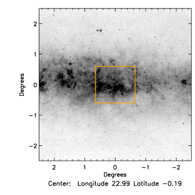
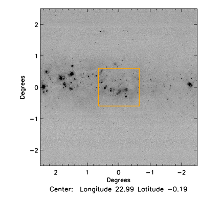
Figure 1: Top: MSX band A (8 $\mu$m; left) and band E (20 $\mu$m; right) images of G23.3–0.3. The square indicates the area displayed in the composite image at the bottom. Bottom: False-color composite image of the G23.3–0.3 complex, which was created with GLIMPSE data: 3.6 $\mu$m (blue), 4.5 $\mu$m (green), and 8.0 $\mu$m (red). Contours of the 20 cm emission detected by MAGPIS (White et al. 2005; Helfand et al. 2006) at 0.002, 0.003, 0.004 Jy beam^-1 levels are super-imposed. Galactic longitude is along the x-axis, and Galactic latitude is along the y-axis.

The Galactic giant molecular cloud (GMC) GMC G23.3$-$0.3 (object ”[23,78]” in Dame et al. (1986)) is found at a distance of 4–5 kpc (Albert et al. 2006). A remarkable number of candidate stellar clusters appear associated with this region (e.g. Messineo et al. 2010), and four SNRs (G$22.9917-0.3583$, G022.7$-$00.2, W41, and G22.7583$-$0.4917, Green 2009; Helfand et al. 2006; Leahy & Tian 2008) are projected against it (as shown by Messineo et al. 2010). The presence of SNRs suggests that massive star formation has been active in multiple sites of this GMC, as do the stellar cluster number 9 in Mercer et al. (2005) (hereafter GLIMPSE9, Messineo et al. 2010), cluster number 10 in Mercer et al. (2005) (hereafter GLIMPSE10), $[BDS2003]$117, and $[BDS2003]$118 (Bica et al. 2003). Additional regions with massive stars were identified by Messineo et al. (2010).

Given this, G23.3$-$0.3 appears to be an ideal laboratory for the investigation of massive stars and multi-seeded star formation. The rich star clusters associated with the complex allow us to study the mode and progression of star formation in this region and to sample rare evolutionary phases of massive stars, such as Wolf-Rayets (WRs), red supergiants (RSGs), and luminous blue variables (LBVs). The presence of supernova remnants (SNRs) indicates that star formation has been progressing for some time, with the current stellar population providing information on the initial masses of the supernova progenitors, and on the fate of massive stars.

In this paper, we present the result of a spectroscopic survey of selected bright stars in the direction of GMC G23.3$-$0.3. In Sect. 2, the spectroscopic observations and data reduction are presented, along with available photometric data. In Sect. 3, we describe the spectral types, the reddening properties, and the selection of massive stars likely associated with the GMC. Luminosities of the massive stars are derived. Eventually, in Sect. 4, we summarize the results, and briefly discuss the spatial distribution of the detected massive stars, their ages, and their connection with the supernova remnants.

2 Observations and data reduction

Table 1: Surveyed regions (see Table 4 of Messineo et al. 2010) and supernova remnants.

Overdensity	RA[J2000]	DEC[J2000]	Rad (′)	SNR	Reference
REG1/ [BDS2003]118	18 34 15.1	$-$08 20 42	1.2	G23.5667$-$0.0333 (SNR5)	1
GLIMPSE9Large	18 34 09.6	$-$09 13 53	3.0a	border of G22.7$-$0.2 (SNR2)	new
				near G22.7583$-$0.4917 (SNR3)
GLIMPSE9 (cluster)	18 34 09.6	$-$09 13 53	0.3		2, 3
REG2	18 34 41.1	$-$08 34 22	4.0	border of W41	2
REG4/GLIMPSE10	18 34 31.6	$-$08 46 47	5.0	core of W41	2, 3
REG5	18 34 20.0	$-$08 59 48	5.0	G22.9917$-$0.3583 (SNR4)	2
REG7/[BDS2003]117	18 34 27.7	$-$09 15 52	2.0b	core of G22.7583$-$0.4917 (SNR3)	2, 1
RSGCX1	18 33 08.9	$-$09 09 14	4.5	core of G22.7$-$0.2 (SNR2)	new

• Notes. ^aA larger region enclosing the GLIMPSE9 cluster was surveyed.   ^b The quoted radius encloses only the bulk of the nebulosity seen at 3.6 $\mu$m.

• References. (1) Bica et al. (2003);  (2) Messineo et al. (2010);  (3) Mercer et al. (2005).

2.1 SINFONI data

The observations were made with the Spectrograph for INtegral Field Observations in the Near Infrared (SINFONI) (Eisenhauer et al. 2003) on the Yepun Very Large Telescope, under the ESO programs 084.D-0769 and 085.D-0192 (P.I. Messineo). We observed $\sim 100$ stars with $0.6<H-$K_s$<1.4$ mag and $11<$K_s$<6$ mag from selected fields (see Table 1); their color-color distribution is shown in Sect. 3.2. A total number of 89 data-cubes were obtained, and a total number of 104 stellar spectra were extracted from these cubes.

We used SINFONI in non-AO mode, with a pixel scale of $0\hbox to0.0pt{.\hss}^{\prime\prime}250$ pix^-1, the $K$-grating (1.95-2.45 $\mu$m), and a resolving power R $\approx 4400$.

Exposures were taken in a target-sky-sky-target sequence, using a fixed sky position. Integration times ($DIT\times NDIT$) ranged from 1 s to 53 s in period 84, and from 1 s to 93 s in period 85. Two exposures were taken for each position. Telluric standard stars of B-type were observed at an airmass within 0.2 dex from the airmass of the science observations, and immediately before or after the science observation.

Data reduction was performed as described in Messineo et al. (2007). The construction of a wavelength-calibrated data-cube, along with the removal of the instrumental signatures, was performed with version 3.9.0 of the ESO SINFONI pipeline (Schreiber et al. 2004; Modigliani et al. 2007). Each science frame was sky-subtracted, and flat-fielded. Dead/hot pixels were removed by interpolation; geometric distortions were corrected. A wavelength-calibration map was obtained using daytime arc-lamp lines. Possible shifts in wavelengths (up to 0.4 pixels) were checked, and corrected with observed OH sky lines (Oliva & Origlia 1992; Rousselot et al. 2000) by cross-correlating the OH line positions with a template spectrum with OH lines at zero velocity.

Stellar traces were extracted from the cubes, and corrected for atmospheric and instrumental responses by dividing the spectra of the targets by the spectra of B-type stars. The Br_γ and He I lines were removed from the spectra of the standards with a linear interpolation, and the resulting spectra were multiplied by a black body curve, F$(_{\lambda})$, with the effective temperature of the star. Some spectra with low signal-to-noise displayed residuals of OH sky lines; in these seven stars, we removed the residuals of the OH sky lines at 2.0008 $\mu$m, 2.0276 $\mu$m, 2.0413 $\mu$m, 2.0563 $\mu$m, 2.0729 $\mu$m, 2.1506 $\mu$m, 2.1802 $\mu$m, 2.1955 $\mu$m, 2.2126 $\mu$m, and 2.2312 $\mu$m with a linear interpolation. The absolute coordinates of the SINFONI fields generally agree with the 2MASS coordinates within 1^′′ or 2^′′. The astrometry of each field was aligned with a 2MASS image or UKIDSS image.

We examined stellar traces with a signal-to-noise ratio above 20-40.

Table 2 lists the early-type stars, and Tables 3 and 12 list the late-type stars. Finding charts are provided in Appendix C.

Table 2: List of detected early-type stars.

ID	Coordinates			Spectral Detection		($J-$Ks)o	($H-$Ks)o	Comment
	RA(J2000)	DEC(J2000)	Instr.	Spectrum	Teff
	[hh mm ss]	[deg mm ss]			[K]
1	18 33 18.14	$-09$ 24 09.9	SofI	OBe	24300$\pm$ 8800	-0.12	-0.06
2	18 33 52.19	$-09$ 10 38.2	SofI	O9-9.5e	29300$\pm$ 1800	-0.16	-0.07	BD$-09$4766
3	18 34 00.86	$-09$ 15 41.5	SINFONI	O6-7fK+	35700$\pm$ 1000	-0.21	-0.10
4	18 34 05.74	$-09$ 16 00.6	SINFONI	O7-8.5fK+	31800$\pm$ 1500	-0.21	-0.10
5	18 34 06.25	$-09$ 15 17.9	SINFONI	O6-7fK+	35700$\pm$ 1000	-0.21	-0.10
6	18 34 08.75	$-09$ 13 59.9	SINFONI	B0-3	23800$\pm$ 6700	-0.16	-0.08
7	18 34 09.25	$-09$ 03 06.0	SINFONI	B4-A2	12700$\pm$ 3600	-0.02	0.00
8	18 34 10.50	$-09$ 14 04.4	SINFONI	B0-3	23800$\pm$ 6700	-0.16	-0.08
9	18 34 10.59	$-09$ 13 43.9	SINFONI	O7-8.5fK+	33100$\pm$ 1500	-0.21	-0.10
10	18 34 10.70	$-09$ 13 58.7	SINFONI	OF	$..$	-0.06	-0.01
11	18 34 11.30	$-09$ 13 56.4	SINFONI	OF	$..$	-0.06	-0.01
12	18 34 11.81	$-08$ 55 44.9	SINFONI	B4-A2	12700$\pm$ 3600	-0.02	0.00
13	18 34 12.14	$-09$ 00 23.6	SINFONI	B4-A2	12700$\pm$ 3600	-0.02	0.00
14	18 34 12.17	$-09$ 12 29.9	SINFONI	O6-7fK+	34500$\pm$ 1200	-0.21	-0.10
15	18 34 13.47	$-09$ 14 31.9	SINFONI	O6-7fK+	34500$\pm$ 1200	-0.21	-0.10
16	18 34 14.47	$-08$ 44 22.9	SINFONI	O9-9.5e	29300$\pm$ 1800	-0.16	-0.07
17	18 34 15.88	$-08$ 45 45.2	SINFONI	O9-9.5fK+	31400$\pm$ 1100	-0.19	-0.09
18	18 34 17.26	$-08$ 46 50.0	SINFONI	O6-7fK+	34500$\pm$ 1200	-0.21	-0.10
19	18 34 18.14	$-08$ 57 18.4	SINFONI	B4-A2	12700$\pm$ 3600	-0.02	0.00
20	18 34 18.85	$-08$ 45 32.9	SINFONI	B4-A2	12700$\pm$ 3600	-0.02	0.00
21	18 34 19.19	$-08$ 46 17.6	SINFONI	B7.5-A2	12900$\pm$ 3900	-0.02	0.00
22	18 34 21.70	$-08$ 28 20.9	SofI	cLBV	13200$\pm$ 2300	0.01	-0.01
23	18 34 23.79	$-08$ 49 18.1	SINFONI	O6-7fK+	35700$\pm$ 1000	-0.21	-0.10
24	18 34 26.38	$-09$ 00 49.1	SINFONI	OF	$..$	-0.06	-0.01
25	18 34 27.67	$-09$ 15 51.1	SINFONI	O4fK+	38200$\pm$ 2500	-0.21	-0.10
26	18 34 28.48	$-08$ 59 31.1	SINFONI	B4-A2	12700$\pm$ 3600	-0.02	0.00
27	18 34 30.15	$-08$ 44 40.6	SINFONI	OF	$..$	-0.06	-0.01
28	18 34 30.84	$-08$ 58 40.1	SINFONI	B4-A2	12700$\pm$ 3600	-0.02	0.00
29	18 34 30.95	$-08$ 58 37.8	SINFONI	OF	$..$	-0.06	-0.01
30	18 34 33.83	$-08$ 32 57.9	SINFONI	OF	$..$	-0.06	-0.01
31	18 34 33.92	$-08$ 32 59.6	SINFONI	B0-3	23800$\pm$ 6700	-0.16	-0.08
32	18 34 35.17	$-09$ 00 39.9	SINFONI	B4-A2	12700$\pm$ 3600	-0.02	0.00
33	18 34 35.74	$-09$ 01 27.6	SINFONI	OF	$..$	-0.06	-0.01
34	18 34 36.94	$-08$ 47 54.7	SINFONI	OF	$..$	-0.06	-0.01
35	18 34 38.36	$-08$ 50 49.7	SINFONI	OF	$..$	-0.06	-0.01
36	18 34 42.63	$-08$ 45 01.9	SINFONI	O6-7fK+	34500$\pm$ 1200	-0.21	-0.10
37	18 34 42.86	$-08$ 45 02.9	SINFONI	OF	$..$	-0.06	-0.01
38	18 34 50.71	$-08$ 46 16.0	SINFONI	B0-3	23800$\pm$ 6700	-0.16	-0.08
$[$MFD2010$]$ 3	18 34 08.68	$-09$ 14 11.1		B0-3	21500$\pm$ 6000	-0.08	-0.04	$[$MFD2010$]$ 3a
$[$MFD2010$]$ 4	18 34 08.54	$-09$ 14 11.8		B0-3	21500$\pm$ 6000	-0.08	-0.04	$[$MFD2010$]$ 4a
$[$MVM2011$]$ 39	18 33 47.64	$-09$ 23 07.7		WC8	65000$\pm$ 5000	0.43	0.38	$[$MVM2011$]$ 39b

• Notes. Identification numbers are followed by celestial coordinates, instrument, spectral types, estimated effective temperatures, T_eff, intrinsic near-infrared colors, and comments. Two B supergiants detected by Messineo et al. (2010), and a WR discovered by Mauerhan et al. (2011) are appended to the table.  We used the collection of infrared colors and temperatures per spectral types as listed in the Appendix of Messineo et al. (2011). For every star (for example a O6-7 star), we assumed the mean temperature of the range considered, and as error half range. (^a) Messineo et al. (2010).  (^b) Mauerhan et al. (2011).

2.2 SofI data

An additional 47 objects were detected with the Son of Isaac (SofI) spectrograph on the ESO New Technology Telescope (NTT) on La Silla during the ESO program 087.D-09609 (P.I, Messineo), on the nights of June 10, 11, and 12, 2011.

Observations with SofI on the NTT were performed with the medium resolution grism, a slit-width of 1^′′, and the K_s filter. A coverage from 2.0 $\mu$m to 2.3 $\mu$m at a resolving power of $\sim 1900$ was obtained. Medium resolution spectra in $H-$band were taken only for one target, a candidate LBV; a slit with a width of 1^′′ was used, which provided a coverage from 1.5 $\mu$m to 1.8 $\mu$m at a resolving power of $\sim 1250$. The objects were nodded along the slit to obtain pairs of frames, which were subtracted and flat-fielded. In a few observations, the stellar traces did not move (no nodding, no jitter), and we subtracted each frame with darks. The two-dimensional frames were rectified with a bilinear interpolation of stellar traces and arc lines. Stellar traces were extracted from individual frames, aligned in wavelength, and co-added. Correction for atmospheric and instrumental responses were performed with spectra of B-type standards (taken in the same manner as for the targets, and with linearly interpolated Br_γ and He I lines). We multiplied the results by a black body curve, F_λ.

Table 3: Spectra of late-type stars that are potential RSGs ($L>4\times 10^{4}$L_⊙  for a distance of 4.6 kpc).

ID	RA(J2000)	DEC(J2000)	Spectral Type							Comment
			Instr.	EW(CO)	Sp[RGB]	Teff[RGB]∗	Sp[RSG]	Teff[RSG]∗	H2O+
	[hh mm ss]	[deg mm ss]		[AA]		[K]		[K]	[%]
39	18 32 36.02	$-$9 08 03.5	SofI	29	M5	3450$\pm$ 203	K5	3869$\pm$ 137	8
40	18 33 08.89	$-$9 08 32.6	SofI	33	$..$	3223$\pm$ 226	M0	3790$\pm$ 124	11	IRAS18303-0910
41	18 33 13.90	$-$9 06 23.2	SofI	23	M1	3745$\pm$ 130	K3	3985$\pm$ 121	0
42	18 33 15.02	$-$9 08 32.2	SofI	23	M1	3745$\pm$ 130	K3	3985$\pm$ 121	10
43	18 33 35.24	$-$8 47 57.7	SofI	32	$..$	3223$\pm$ 226	M0	3790$\pm$ 124	18	BGa
44	18 33 37.80	$-$9 21 38.1	SofI	21	M0	3790$\pm$ 124	K2	4049$\pm$ 131	8
45	18 33 40.98	$-$9 03 25.2	SofI	26	M3	3605$\pm$ 120	K3	3985$\pm$ 121	$-$16
46	18 34 10.36	$-$9 13 52.9	SINFONI	64	$..$	3223$\pm$ 226	M3	3605$\pm$ 120	$-$76	[MFD2010]8b
47	18 34 23.17	$-$8 48 38.6	SINFONI	61	$..$	3223$\pm$ 226	M2	3660$\pm$ 140	$-$6
48	18 34 33.86	$-$8 44 21.2	SINFONI	47	M6	3336$\pm$ 226	K5	3869$\pm$ 137	$-$16
$[$MFD2010$]$ 5	18 34 09.86	$-$9 14 23.8	SINFONI	$..$	$..$	3223$\pm$ 226	M1.5	3710$\pm$ 152	$..$	$[$MFD2010$]$ 5b
BD$-$08 4635	18 34 51.88	$-$8 36 40.8	SINFONI	$..$	$..$	3223$\pm$ 226	M2	3660$\pm$ 140	$..$	BD$-$08 4635c
BD$-$08 4639	18 35 31.06	$-$8 41 23.4	SINFONI	$..$	$..$	3223$\pm$ 226	K2	4049$\pm$ 131	$..$	BD$-$08 4639c
BD$-$08 4645	18 36 21.66	$-$8 52 40.0	SINFONI	$..$	$..$	3223$\pm$ 226	M2	3660$\pm$ 140	$..$	BD$-$08 4645c

• Notes. Identification numbers are followed by celestial coordinates, instrument, EW(CO)s, spectral types, T_eff, H₂O indexes, and comments. Two spectral types are reported; the first was obtained using the relation for red giants (Sp[RGB]), the latter using that for red supergiants (Sp[RSG]). We appended to the table RSG [MFD2010]5 (Messineo et al. 2010), RSG BD$-08$ 4645, BD$-08$ 4635, and BD$-08$ 4639 (Skiff 2013).   (^∗) Temperature errors account for accuracy in spectral types of $\pm 2$.  (⁺) The H₂O index depends on the correction for A${}_{\it K_{\rm s}}$; a variation of 10% in A${}_{\it K_{\rm s}}$ typically affects the H₂O by 20%. (^a) BG= object in the background of the cloud.  (^b) Messineo et al. (2010).  (^c) Skiff (2013).

2.3 Infrared photometry

We searched for counterparts of the observed stars in the 2MASS Catalog of Point Sources (Cutri et al. 2003), in the third release of DENIS data at CDS (catalog B/denis) (Epchtein et al. 1994), in the GLIMPSE catalog (Churchwell et al. 2009), and in the WISE catalog (Cutri & et al. 2012); we used the closest match within a search radius of 2^′′. We searched in the UKIDSS catalog (Lucas et al. 2008) with a search radius of 1^′′, and retained only counterparts in the linear regime ($K\ga 10.2$ mag). The II/293 (GLIMPSE) catalog from CDS is a combination of the original GLIMPSE-I (v2.0), GLIMPSE-II (v2.0), and GLIMPSE-3D catalogs. We also searched for counterparts in the Version 2.3 of the MSX Point Source Catalog (Egan et al. 2003; Price et al. 2001) with a search radius of 5^′′. MSX upper limits were removed. WISE counterparts were retained only if their signal-to-noise ratio was larger than 2.0. Near-infrared and GLIMPSE counterparts were visually checked with 2MASS/UKIDSS and GLIMPSE charts. For most of sources, WISE band-3 and band-4 provided upper limit magnitudes, due to confusion.

In addition, we searched for possible $B$, $V$, $R$-band matches in The Naval Observatory Merged Astrometric Dataset (NOMAD) by Zacharias et al. (2004). The photometric data are listed in Table 4. For a few targets (missing in both 2MASS and UKIDSS), K_s counterparts were estimated from the SINFONI cubes (with a typical uncertainty of $\sim 0.3$ mag). For stars [MFD2010]3, [MFD2010]4, and [MFD2010]5, $H$ and $K$-band measurements were obtained with the Near Infrared Camera and Multi-Object Spectrometer (NICMOS, Skinner et al. 1998) (Messineo et al. 2010).

Table 4: Infrared measurements of the spectroscopically detected early-type stars and candidate RSGs.

	2MASSa			DENIS			UKIDSSb			GLIMPSE				MSX	WISE				NOMAD
IDf	J	H	$K_{\mathrm{s}}$	I	J	$K_{\mathrm{s}}$	J	H	$K$	[3.6]	[4.5]	[5.8]	[8.0]	A	W1	W2	W3	W4	R
	[mag]	[mag]	[mag]	[mag]	[mag]	[mag]	[mag]	[mag]	[mag]	[mag]	[mag]	[mag]	[mag]	[mag]	[mag]	[mag]	[mag]	[mag]	[mag]
1	9.66	9.35	9.17	10.49	9.77	9.20	$..$	$..$	$..$	9.07	8.89	8.70	8.44	$..$	8.98	8.85	$..$	7.06	10.82
2	7.35	6.84	6.61	9.13	6.90	6.58	$..$	$..$	$..$	6.86	6.46	6.32	6.38	$..$	6.39	6.33	6.25	3.72	9.85
3	14.01	11.85	10.75	$..$	13.98	10.83	13.99	11.88	10.76	10.05	9.82	9.65	9.97	$..$	10.14	9.86	8.58	5.66	$..$
4	12.73	10.91	9.88	$..$	12.75	9.87	$..$	$..$	$..$	9.33	9.06	8.96	8.98	$..$	9.23	8.89	7.52	5.46	$..$
5	13.30	11.35	10.38	$..$	13.23	10.30	13.25	11.40	10.35	9.63	9.51	9.31	9.40	$..$	9.59	9.30	8.48	5.85	$..$
6	13.15	11.43	10.53	$..$	13.09	10.26	13.47	12.47	10.74	$..$	$..$	$..$	$..$	$..$	$..$	$..$	$..$	$..$	$..$
7	11.71	11.22	10.96	13.28	11.66	10.90	11.75	11.60	10.97	10.81	10.71	10.61	10.29	$..$	10.80	10.88	$..$	4.04	14.16
8c	$..$	$..$	$..$	$..$	14.91	12.11	14.91	13.01	12.01	$..$	$..$	$..$	$..$	$..$	$..$	$..$	$..$	$..$	$..$
9	13.43	11.45	10.40	$..$	13.34	10.39	13.48	11.55	10.50	9.77	$..$	9.48	9.50	$..$	$..$	$..$	$..$	$..$	$..$
10c	$..$	$..$	$..$	$..$	$..$	$..$	16.31	14.16	13.12	$..$	$..$	$..$	$..$	$..$	$..$	$..$	$..$	$..$	$..$
11c	$..$	$..$	$..$	$..$	$..$	$..$	17.70	15.86	15.06	$..$	$..$	$..$	$..$	$..$	$..$	$..$	$..$	$..$	$..$
12	10.93	10.57	10.39	$..$	$..$	$..$	11.15	12.00	10.48	10.40	10.31	10.29	10.24	$..$	10.05	9.97	$..$	4.60	12.62
13	10.84	10.51	10.38	11.74	10.81	10.34	10.98	10.85	10.41	10.28	10.25	10.23	10.20	$..$	10.20	10.28	$..$	2.22	12.72
14	13.36	11.25	10.18	$..$	13.22	10.11	$..$	$..$	$..$	9.51	9.11	8.89	8.89	$..$	9.47	8.87	6.98	2.36	$..$
15	12.21	10.42	9.52	$..$	12.10	9.44	$..$	$..$	$..$	8.93	8.73	8.63	8.75	$..$	8.96	8.73	$..$	4.66	$..$
16	12.07	10.15	9.19	$..$	12.03	9.10	$..$	$..$	$..$	8.38	8.22	8.02	7.99	$..$	8.46	8.15	6.25	3.96	$..$
17	12.90	11.37	10.58	18.13	12.90	10.47	12.90	11.53	10.61	10.00	9.89	9.87	9.76	$..$	9.89	9.66	$..$	$..$	$..$
18	12.46	10.72	9.96	$..$	12.36	9.80	$..$	$..$	$..$	9.27	9.08	9.02	9.07	$..$	9.33	9.08	$..$	4.66	$..$
19	11.06	10.58	10.36	12.32	11.12	10.27	11.17	11.09	10.36	10.22	10.17	10.15	$..$	$..$	10.25	9.98	7.02	$..$	13.41
20c	$..$	$..$	$..$	14.50	13.29	11.93	13.06	12.52	12.42	$..$	$..$	$..$	$..$	$..$	$..$	$..$	$..$	$..$	$..$
21	12.73	11.42	10.76	17.20	12.61	10.64	12.72	11.59	10.74	10.29	10.15	10.02	10.02	$..$	10.37	10.18	$..$	$..$	$..$
22	9.78	8.42	7.63	13.92	9.67	7.51	$..$	$..$	$..$	6.89	6.51	6.17	5.93	5.95	6.85	6.40	5.74	4.41	16.75
23	12.75	11.20	10.43	17.90	12.77	10.38	12.69	11.20	10.38	9.83	9.66	9.55	9.93	$..$	10.05	9.87	$..$	2.19	$..$
24d	$..$	$..$	14.66	$..$	$..$	$..$	$..$	$..$	$..$	$..$	$..$	$..$	$..$	$..$	$..$	$..$	$..$	$..$	$..$
25	12.16	10.67	9.90	$..$	12.34	10.16	$..$	$..$	$..$	9.44	9.12	9.02	$..$	$..$	$..$	$..$	$..$	$..$	$..$
26	11.27	10.92	10.73	12.63	11.57	10.98	11.54	11.36	10.74	10.60	10.50	10.25	9.74	$..$	10.76	10.76	$..$	3.22	13.29
27d	$..$	$..$	14.16	$..$	$..$	$..$	15.01	13.94	$..$	$..$	$..$	$..$	$..$	$..$	$..$	$..$	$..$	$..$	16.22
28	11.38	11.04	10.78	12.80	11.67	11.06	11.60	11.43	10.84	10.69	10.67	10.12	$..$	$..$	10.40	10.05	5.81	2.95	13.81
29c	$..$	$..$	$..$	$..$	$..$	$..$	15.26	14.53	14.30	$..$	$..$	$..$	$..$	$..$	$..$	$..$	$..$	$..$	$..$
30c	$..$	$..$	$..$	$..$	$..$	$..$	15.17	13.59	12.85	$..$	$..$	$..$	$..$	$..$	$..$	$..$	$..$	$..$	$..$
31	12.50	11.07	10.32	17.75	12.77	10.67	12.49	11.31	10.39	9.80	9.81	9.79	$..$	$..$	9.52	9.31	5.93	3.32	$..$
32	11.22	10.79	10.57	12.87	11.58	10.77	11.50	11.34	10.61	10.40	10.31	$..$	$..$	$..$	10.29	10.14	$..$	3.83	13.38
33d	$..$	$..$	13.25	15.02	$..$	$..$	13.66	12.79	$..$	$..$	$..$	$..$	$..$	$..$	$..$	$..$	$..$	$..$	15.66
34d	$..$	$..$	12.79	$..$	$..$	$..$	$..$	$..$	$..$	$..$	$..$	$..$	$..$	$..$	$..$	$..$	$..$	$..$	18.15
35c	13.71	$..$	$..$	$..$	$..$	$..$	13.81	13.18	13.01	$..$	$..$	$..$	$..$	$..$	$..$	$..$	$..$	$..$	15.26
36	13.37	11.18	10.06	$..$	13.64	10.33	$..$	$..$	$..$	9.26	9.04	8.92	9.00	$..$	9.27	8.90	6.07	0.90	$..$
37c	$..$	$..$	$..$	$..$	$..$	$..$	15.88	13.52	12.40	$..$	$..$	$..$	$..$	$..$	$..$	$..$	$..$	$..$	$..$
38	12.40	11.13	10.50	17.13	12.71	10.81	12.35	11.18	10.52	10.07	9.92	9.63	10.24	$..$	9.88	9.68	7.12	3.96	$..$
$[$MFD2010$]$ 3e	10.66	8.93	7.96	17.06	10.50	7.63	$..$	$..$	$..$	6.46	6.81	6.47	6.63	$..$	6.59	6.31	6.65	4.71	$..$
$[$MFD2010$]$ 4e	$..$	10.21	9.14	$..$	$..$	$..$	$..$	$..$	$..$	$..$	$..$	$..$	$..$	$..$	$..$	$..$	$..$	$..$	$..$
$[$MVM2011$]$ 39	12.18	10.52	9.36	17.77	12.20	9.42	$..$	$..$	$..$	8.53	8.03	7.78	7.51	$..$	8.67	8.06	7.57	$..$	$..$
39	7.36	5.62	4.84	$..$	$..$	4.11	$..$	$..$	$..$	4.31	4.67	4.22	4.26	4.15	4.54	4.06	4.28	3.78	$..$
40	9.71	6.66	5.08	$..$	9.61	4.27	$..$	$..$	$..$	4.00	4.31	3.62	3.22	3.15	4.95	3.40	2.32	0.97	$..$
41	9.60	7.45	6.52	15.73	9.48	6.49	$..$	$..$	$..$	6.73	6.05	5.75	5.68	5.68	6.06	5.92	5.62	3.94	$..$
42	8.79	6.93	6.14	13.59	8.72	5.90	$..$	$..$	$..$	6.66	5.95	5.56	5.54	5.58	5.63	5.57	5.86	$..$	17.22
43	$..$	10.49	7.91	17.14	14.97	7.95	$..$	$..$	$..$	6.77	6.41	5.54	5.61	$..$	6.47	5.98	6.32	$..$	$..$
44	8.69	6.73	5.84	14.33	8.64	5.07	$..$	$..$	$..$	7.40	5.97	5.16	5.16	5.07	5.42	5.29	5.21	4.04	$..$
45	9.41	7.25	6.21	16.20	9.30	6.16	$..$	$..$	$..$	5.60	6.18	5.33	5.26	5.15	5.66	5.41	4.85	3.74	$..$
46	10.22	7.59	6.29	$..$	10.02	6.25	$..$	$..$	$..$	5.38	$..$	4.89	4.78	$..$	5.05	4.91	4.14	2.47	$..$
47	9.59	7.32	6.19	16.63	9.59	6.23	$..$	$..$	$..$	5.52	6.12	5.30	5.30	4.95	5.56	5.37	4.91	2.95	$..$
48	9.03	7.00	6.06	15.90	9.44	6.30	$..$	$..$	$..$	$..$	$..$	5.24	5.25	5.16	$..$	$..$	$..$	$..$	$..$
$[$MFD2010$]$ 5e	11.41	8.43	7.05	$..$	11.32	6.97	$..$	$..$	$..$	6.75	7.39	5.70	5.84	$..$	6.09	5.97	6.26	4.34	$..$
BD$-$08 4635	4.79	3.45	3.05	8.57	$..$	3.73	$..$	$..$	$..$	$..$	3.91	$..$	$..$	2.75	3.04	2.51	2.92	2.87	9.90
BD$-$08 4639	4.05	3.06	2.77	8.69	$..$	3.85	$..$	$..$	$..$	$..$	$..$	$..$	$..$	2.84	$..$	$..$	$..$	$..$	8.05
BD$-$08 4645	3.92	2.73	2.29	8.97	$..$	3.89	$..$	$..$	$..$	$..$	$..$	$..$	$..$	2.40	$..$	$..$	$..$	$..$	10.69

• Notes. (${\mathrm{a}}$) 2MASS upper limits and confused stars were removed all, but star #4.  (${\mathrm{b}}$) Small corrections ($J\approx+0.1$ mag, $H\approx-0.1$ mag, $K\approx 0.0$ mag) were applied to match the 2MASS photometric system.  (${\mathrm{c}}$) UKIDSS values were used.  (${\mathrm{d}}$) K_s was estimated from the SINFONI data-cube.  (${\mathrm{e}}$) $H$ and K_s were taken from Messineo et al. (2010).  (${\mathrm{f}}$) Identification numbers are taken from Table 2, 3, and 12.

Table 4: continuation of Table 4. Associated errors.

	2MASS			DENIS			UKIDSS			GLIMPSE				MSX	WISE
ID	$J_{\mathrm{e}rr}$	$H_{\mathrm{e}rr}$	$K_{\mathrm{s}err}$	$I_{\mathrm{e}rr}$	$J_{\mathrm{e}rr}$	$K_{\mathrm{s}err}$	$J_{\mathrm{e}rr}$	$H_{\mathrm{e}rr}$	$K_{\mathrm{e}rr}$	[3.6err]	[4.5err]	[5.8err]	[8.0err]	Aerr	W1err	W2err	W3err	W4err
	[mag]	[mag]	[mag]	[mag]	[mag]	[mag]	[mag]	[mag]	[mag]	[mag]	[mag]	[mag]	[mag]	[mag]	[mag]	[mag]	[mag]	[mag]
1	0.02	0.02	0.02	0.03	0.07	0.07	$..$	$..$	$..$	0.04	0.05	0.05	0.03	$..$	0.03	0.02	$..$	0.48
2	0.02	0.03	0.02	0.06	0.16	0.09	$..$	$..$	$..$	0.05	0.07	0.03	0.03	$..$	0.04	0.02	0.05	0.35
3	0.03	0.02	0.02	$..$	0.12	0.08	0.002	0.001	0.001	0.05	0.06	0.06	0.08	$..$	0.04	0.03	0.31	0.23
4	$..$	$..$	$..$	$..$	0.10	0.08	$..$	$..$	$..$	0.07	0.05	0.05	0.05	$..$	0.03	0.03	0.18	0.31
5	0.02	0.02	0.03	$..$	0.10	0.08	0.001	$..$	0.001	0.03	0.05	0.05	0.05	$..$	0.03	0.03	0.35	0.15
6	0.12	0.02	0.02	$..$	0.10	0.08	0.001	0.001	0.001	$..$	$..$	$..$	$..$	$..$	$..$	$..$	$..$	$..$
7	0.03	0.03	0.02	0.03	0.09	0.08	0.001	0.001	0.001	0.05	0.06	0.08	0.10	$..$	0.04	0.06	$..$	0.07
8	$..$	$..$	$..$	$..$	0.14	0.10	0.003	0.001	0.001	$..$	$..$	$..$	$..$	$..$	$..$	$..$	$..$	$..$
9	0.05	0.06	0.09	$..$	0.10	0.08	0.001	$..$	0.001	0.07	$..$	0.05	0.06	$..$	$..$	$..$	$..$	$..$
10	$..$	$..$	$..$	$..$	$..$	$..$	0.009	0.003	0.003	$..$	$..$	$..$	$..$	$..$	$..$	$..$	$..$	$..$
11	$..$	$..$	$..$	$..$	$..$	$..$	0.030	0.014	0.016	$..$	$..$	$..$	$..$	$..$	$..$	$..$	$..$	$..$
12	0.03	0.03	0.03	$..$	$..$	$..$	$..$	0.001	0.001	0.06	0.05	0.08	0.09	$..$	0.03	0.04	$..$	0.08
13	0.02	0.02	0.02	0.03	0.08	0.08	$..$	$..$	0.001	0.05	0.06	0.07	0.16	$..$	0.04	0.09	$..$	0.03
14	0.03	0.03	0.02	$..$	0.10	0.08	$..$	$..$	$..$	0.06	0.06	0.04	0.08	$..$	0.03	0.02	0.06	0.04
15	0.03	0.03	0.02	$..$	0.09	0.07	$..$	$..$	$..$	0.04	0.05	0.04	0.05	$..$	0.03	0.03	$..$	0.07
16	0.03	0.02	0.02	$..$	0.09	0.07	$..$	$..$	$..$	0.03	0.05	0.04	0.06	$..$	0.03	0.03	0.06	0.14
17	0.02	0.03	0.03	0.19	0.10	0.08	0.001	$..$	0.001	0.07	0.06	0.07	0.07	$..$	0.03	0.03	$..$	$..$
18	0.02	0.02	0.02	$..$	0.09	0.08	$..$	$..$	$..$	0.05	0.05	0.03	0.06	$..$	0.03	0.03	$..$	0.29
19	0.02	0.02	0.02	0.03	0.08	0.08	$..$	$..$	$..$	0.05	0.06	0.08	$..$	$..$	0.05	0.05	0.14	$..$
20	$..$	$..$	$..$	0.06	0.09	0.10	0.001	0.001	0.002	$..$	$..$	$..$	$..$	$..$	$..$	$..$	$..$	$..$
21	0.03	0.02	0.02	0.12	0.10	0.08	0.001	0.001	0.001	0.06	0.06	0.06	0.09	$..$	0.05	0.05	$..$	$..$
22	0.03	0.04	0.03	0.06	0.05	0.06	$..$	$..$	$..$	0.03	0.06	0.03	0.03	0.05	0.03	0.02	0.06	0.17
23	0.03	0.03	0.02	0.17	0.10	0.08	0.001	$..$	0.001	0.04	0.06	0.05	0.09	$..$	0.04	0.04	$..$	0.06
24	$..$	$..$	0.30	$..$	$..$	$..$	$..$	$..$	$..$	$..$	$..$	$..$	$..$	$..$	$..$	$..$	$..$	$..$
25	0.03	0.03	0.02	$..$	0.09	0.08	$..$	$..$	$..$	0.06	0.10	0.11	$..$	$..$	$..$	$..$	$..$	$..$
26	0.02	0.02	0.02	0.04	0.08	0.08	$..$	$..$	0.001	0.04	0.08	0.08	0.15	$..$	0.07	0.11	$..$	0.11
27	$..$	$..$	0.30	$..$	$..$	$..$	0.003	0.002	$..$	$..$	$..$	$..$	$..$	$..$	$..$	$..$	$..$	$..$
28	0.03	0.03	0.03	0.04	0.08	0.08	$..$	$..$	0.001	0.08	0.09	0.10	$..$	$..$	0.05	0.08	0.10	0.04
29	$..$	$..$	$..$	$..$	$..$	$..$	0.004	0.004	0.008	$..$	$..$	$..$	$..$	$..$	$..$	$..$	$..$	$..$
30	$..$	$..$	$..$	$..$	$..$	$..$	0.003	0.002	0.002	$..$	$..$	$..$	$..$	$..$	$..$	$..$	$..$	$..$
31	0.04	0.05	0.03	0.22	0.09	0.08	0.001	$..$	0.001	0.07	0.09	0.12	$..$	$..$	0.03	0.05	0.05	0.16
32	0.02	0.02	0.04	0.04	0.08	0.08	$..$	$..$	0.001	0.07	0.10	$..$	$..$	$..$	0.08	0.09	$..$	0.38
33	$..$	$..$	0.30	0.07	$..$	$..$	0.001	0.001	$..$	$..$	$..$	$..$	$..$	$..$	$..$	$..$	$..$	$..$
34	$..$	$..$	0.30	$..$	$..$	$..$	$..$	$..$	$..$	$..$	$..$	$..$	$..$	$..$	$..$	$..$	$..$	$..$
35	0.05	$..$	$..$	$..$	$..$	$..$	0.001	0.001	0.003	$..$	$..$	$..$	$..$	$..$	$..$	$..$	$..$	$..$
36	0.02	0.03	0.02	$..$	0.10	0.08	$..$	$..$	$..$	0.05	0.05	0.06	0.04	$..$	0.03	0.03	0.06	0.05
37	$..$	$..$	$..$	$..$	$..$	$..$	0.006	0.002	0.002	$..$	$..$	$..$	$..$	$..$	$..$	$..$	$..$	$..$
38	0.03	0.02	0.02	0.16	0.09	0.08	0.001	$..$	0.001	0.07	0.06	0.06	0.16	$..$	0.03	0.04	0.07	0.10
$[$MFD2010$]$ 3	0.04	0.02	0.30	0.11	0.08	0.07	$..$	$..$	$..$	0.15	0.17	0.04	0.05	$..$	0.04	0.02	0.09	0.08
$[$MFD2010$]$ 4	$..$	0.02	0.02	$..$	$..$	$..$	$..$	$..$	$..$	$..$	$..$	$..$	$..$	$..$	0.04	0.02	0.09	0.08
$[$MVM2011$]$ 39	0.02	0.02	0.02	0.16	0.09	0.07	$..$	$..$	$..$	0.04	0.05	0.03	0.03	$..$	0.03	0.02	0.10	$..$
39	0.02	0.03	0.02	$..$	$..$	0.21	$..$	$..$	$..$	0.06	0.04	0.02	0.03	0.05	0.10	0.05	0.02	0.07
40	0.02	0.04	0.02	$..$	0.07	0.21	$..$	$..$	$..$	0.06	0.05	0.03	0.02	0.05	0.07	0.07	0.02	0.02
41	0.02	0.04	0.02	0.06	0.06	0.11	$..$	$..$	$..$	0.12	0.05	0.03	0.02	0.05	0.04	0.02	0.03	0.04
42	0.03	0.04	0.02	0.03	0.07	0.16	$..$	$..$	$..$	0.10	0.05	0.04	0.03	0.05	0.05	0.03	0.04	$..$
43	$..$	0.03	0.03	0.12	0.15	0.06	$..$	$..$	$..$	0.11	0.08	0.03	0.02	$..$	0.04	0.02	0.08	$..$
44	0.04	0.04	0.02	0.04	0.07	0.20	$..$	$..$	$..$	0.30	0.11	0.02	0.03	0.05	0.05	0.03	0.02	0.05
45	0.02	0.04	0.02	0.08	0.07	0.11	$..$	$..$	$..$	0.05	0.09	0.03	0.03	0.05	0.05	0.03	0.03	0.06
46	0.03	0.05	0.02	$..$	0.07	0.10	$..$	$..$	$..$	0.06	$..$	0.03	0.03	$..$	0.06	0.03	0.02	0.03
47	0.02	0.03	0.02	0.09	0.07	0.11	$..$	$..$	$..$	0.10	0.10	0.03	0.03	0.05	0.05	0.03	0.03	0.06
48	0.02	0.03	0.03	0.10	0.07	0.12	$..$	$..$	$..$	$..$	$..$	0.03	0.02	0.05	$..$	$..$	$..$	$..$
$[$MFD2010$]$ 5	0.02	0.03	0.03	$..$	0.08	0.08	$..$	$..$	$..$	0.08	0.23	0.03	0.02	$..$	0.06	0.02	0.07	0.05
BD$-$08 4635	0.24	0.22	0.26	0.05	$..$	0.15	$..$	$..$	$..$	$..$	0.18	$..$	$..$	0.05	0.11	0.06	0.02	0.03
BD$-$08 4639	0.22	0.18	0.22	0.02	$..$	0.16	$..$	$..$	$..$	$..$	$..$	$..$	$..$	0.05	0.12	0.08	0.02	0.05
BD$-$08 4645	0.21	0.18	0.19	0.04	$..$	0.17	$..$	$..$	$..$	$..$	$..$	$..$	$..$	0.05	0.31	0.14	0.03	0.03

2.4 Previously known massive stars in the direction of the complex

In the SIMBAD astronomical archive, we found matches for 11 out of 151 observed stars. The alias names are provided in Tables 2, 3, and 12.

Messineo et al. (2010) reported the detections of a few massive stars in the direction of the GLIMPSE9 cluster; [MFD2010]3 and [MFD2010]4 are two B0-5 supergiants; [MFD2010]5 and [MFD2010]8 are two RSG stars. Our detection number #46 coincides with star [MFD2010]8.

We searched the lists of known WRs presented by van der Hucht (2001), Mauerhan et al. (2011), and Shara et al. (2012). The WR number 39 (WC8) in Mauerhan et al. (2011) (thereafter, we call it [MVM2011]39) is projected onto SNR G22.07$-$0.3.

We searched in the Galactic spectroscopic database by Skiff (2013) for known RSGs. BD$-08$ 4645 (EIC 685) is reported as a M2 I by Whitney (1983) and Sylvester et al. (1998). BD$-08$ 4635 and BD$-08$ 4639 are two bright sources with IR colors similar to that of RSG BD$-08$ 4645. Skiff (2013) lists them as M2 and K2 types, respectively.

These massive stars and candidate massive stars were added to the list of newly detected stars, and their photometric properties were re-investigated.

3 Results

3.1 Spectral classification

3.1.1 Early-type stars

Figure 2: Normalized spectra (arbitrarily shifted for clarity) of detected early-type stars. The positions of lines from H I, He I, and He II are marked and labeled at the top, along with those of other detected lines from Si IV, N III, and C IV. The spectra were multiplied by the black body of the standard star. Dotted lines show black bodies with the temperatures inferred from the observed stellar spectral types; these black bodies were reddened with individual A${}_{\it K_{\rm s}}$ values (for details see Section 3.2).

A total number of 38 early-type stars were detected (see Figs. 2 and 3). We classified them by comparison with infrared spectroscopic atlases (e.g. Hanson et al. 1996; Morris et al. 1996; Figer et al. 1997; Hanson et al. 2005), by using H I, He I, He II, N III, and C IV lines. C IV lines are typical of O4-7 types, more rarely appear in O8 type; the N III complex at 2.115 $\mu$m disappears in stars later than O8.5-O9 type; the He II line at 2.189 $\mu$m is present in O-type stars down to O9-type; the He I line at 2.112 $\mu$m  is observed from O4-type down to B8 (for supergiants), or B3 (for dwarfs), and the strengths of the He I absorption line at 2.112 $\mu$m increases from early-O to late-O. The He I line at 2.058 $\mu$m is usually seen down to $\sim$B3 (Davies et al. 2012).

We used the prefix f_K+ to denote a spectral classification in $K$-band similar to that given in the optical window by Maíz Apellániz et al. (2007) and Fariña et al. (2009). We, thereby, defined an Of_K+ stars as a star with a $K$-band spectrum that shows the N III/C III complex at 2.115 $\mu$m in emission, and Si IV at 2.428 $\mu$m in emission. There are only a few previous reports on the Si IV line at 2.428 $\mu$m; the line was identified in some WRs and O supergiants of the Arches cluster (Martins et al. 2008), and transitional objects (e.g. cLBVs) in the vicinity of the Galactic center (Martins et al. 2007). The detected O-type stars are all Of_K+.

Of_K+ type stars ( panel 1 of Fig. 2):
The spectrum of star #25 shows strong C IV lines at 2.0705 $\mu$m and at 2.0796 $\mu$m in emission, and the broad N III/C III complex at 2.115 $\mu$m in emission, the Br_γ line at 2.1661 $\mu$m in absorption with a wind signature in emission, the He II line at 2.1891 $\mu$m in absorption, and the Si IV line at 2.428 $\mu$m in emission. These lines are typically detected in O stars with types from 4 to 6. In Hanson et al. (1996) and Hanson et al. (2005), the strength of the carbon lines appears to increase with earlier types; therefore, star #25 is likely a O4-5f_K+ supergiant, similar to HD15570 (see spectrum in Hanson et al. 2005).

The spectra of stars #3, #5, #14, #15, #18, #23, and #36 display signatures of O6-7f_K+ stars; they are characterized by the He I line at 2.058 $\mu$m, a weak C IV line at 2.0796 $\mu$m in emission, a prominent He I line at 2.112 $\mu$m in absorption, the N III complex at 2.115 $\mu$m in emission, the Br_γ  (mostly in absorption), the He II line at 2.189 $\mu$m in absorption, and the Si IV line at 2.248 $\mu$m. The spectra of stars #3 and #23 have the additional detection of a C IV line at 2.0705 $\mu$m. The spectrum of star #14 has the Br_γ line in emission (O6-7f_K+); the Br_γ lines of stars #3 and #5 display a wind signature.

The spectra of stars #4 and #9 have the He I lines at 2.058 $\mu$m and 2.112 $\mu$m in absorption, the N III at 2.115 $\mu$m in emission, the Br_γ line, the He II line at 2.189 $\mu$m in absorption, and the Si IV line at 2.428 $\mu$m. Star #4 has a Br_γ line in absorption with a signature of wind in emission. The non-detection of C IV lines, the presence of N III and He II lines, and Si IV suggest a later Of_K+ (O7-O8.5${}^{+}_{K}$).

The spectrum of star #17 displays a He I line at 2.112 $\mu$m in absorption, a weak N III complex at 2.115 $\mu$m  in emission, the Br_γ line in absorption, and the Si IV line at 2.248 $\mu$m in emission. Since there is not He II at 2.189 $\mu$m, but N III emission is still detected, this star appears a (O9-O9.5)f_K+.

Late-O and B type stars ( panel 2 of Fig. 2):

The spectrum of star #1 presents the Br_γ line in emission.

The spectrum of star #2 has the Br_γ line in absorption, and a hint for the He I line at 2.058 $\mu$m in emission, and for the He II line at 2.189 $\mu$m in absorption. The lack of N III at 2.115 $\mu$m, and the hint for He I and He II, suggest a O9-O9.5e.

The spectrum of star #16 shows the He I line at 2.058 $\mu$m in emission, the He I line at 2.112 $\mu$m in absorption, the N III line at 2.115 $\mu$m  in emission, and the Br_γ line in absorption. The absence of He II and presence of N III suggest a O9-9.5 type. The 2.058 $\mu$m emission indicates a supergiant luminosity class (Hanson et al. 1996).

The He I line at 2.112 $\mu$m  and the Br_γ line in absorption are detected in the spectra of stars #6, #8, #31, and #38. The detection of He I lines and the absence of N III emission at 2.115 $\mu$m and of the He II line at 2.189 $\mu$m suggest a B0-8I or a B0-3V. There is a hint for He I at 2.058 $\mu$m in the spectra of stars #6 and #8 (B0-3); there is a hint for Si IV at 2.248 $\mu$m in the spectrum of star #31.

B-A type stars ( panel 3 of Fig. 2):
We assigned a B4-A2 type (dwarfs), or B7.5-A2 type (supergiants) to stars with only a detected Br_γ line in absorption: #7, #12, #13, #19, #20, #21, #26, #28, and #32.

O-B-A-F type stars ( panel 4 of Fig. 2):
Stars with noisy spectra and marginal detections of Br_γ lines are labeled O-B-A-F (stars #10, #11, #24, #27,#29, #30, #33, #34, #35, and #37).

The noisy structures around 2.00 $\mu$m are due to a poor atmospheric correction.

3.1.2 A candidate Luminous Blue Variable.

Table 5: List of lines detected in the new spectra of the cLBV (#22).

Line	Vacuum $\lambda$	Obs. $\lambda$∗	EW+
	[$\mu$m]	[$\mu$m]	[$\AA$]
H I 18-4	1.53460e,f	1.53483	$1.1\pm 0.2$
+$[\rm{{Fe\textsc{II}}}]$ a4F${}_{9/2}-$a4D5/2	1.53389a,f	blended
H I 17-4	1.54432e,f	1.54473	$1.0\pm 0.2$
H I 16-4	1.55607e,f	1.55624	$2.3\pm 0.5$
H I 15-4	1.57049e,f	1.57089	$1.7\pm 0.3$
Fe II $z^{2}$ I${}_{11/2}-$3 d5 4 s2 I11/2	1.5776d	1.57663	$1.6\pm 0.3$
H I 14-4	1.58849e,f	1.58885	$2.0\pm 0.5$
H I 13-4	1.61137e,f	1.61177	$1.5\pm 1.0$
H I 12-4	1.64117e,f	1.64151	$1.9\pm 0.4$
$[\rm{{Fe\textsc{II}}}]$ a4F${}_{9/2}-$a4D7/2	1.64400a,f	1.64457	$0.6\pm 0.1$
$[\rm{{Fe\textsc{II}}}]$ a4F${}_{5/2}-$a4D1/2	1.66422a,f	1.66510	$0.5\pm 0.1$
H I 11-4	1.68111e,f	1.68136	$3.7\pm 0.8$
Fe II $z^{4}$ F${}_{9/2}-$ c4 F9/2	1.68778d,f	1.68814	$1.5\pm 0.4$
$[\rm{{Fe\textsc{II}}}]$ a4F${}_{5/2}-$a4D3/2	1.71159a,f	1.71151	$0.4\pm 0.3$
H I 10-4	1.73669e,f	1.73700	$3.1\pm 0.3$
He I	2.05869d,f	2.05950	$7.8\pm 0.5$
Fe II $z^{4}$ F${}^{0}_{3/2}-$ c4 F3/2	2.091d	2.09009	$0.9\pm 0.3$
Mg II	2.13748d,f	2.13808	$0.6\pm 0.5$ g
Mg II	2.14380d,f	2.14453	$0.3\pm 0.3$ h
H I 7-4	2.16612e,f	2.16691	$15.8\pm 0.4$
Na I	2.206d,f	2.2082	$4.6\pm 0.6$
Na I	2.20897d,f	blended

• (^a) Morris et al. (1996); Reunanen et al. (2007).  (^d) Morris et al. (1996); Clark et al. (1999).  (^e) Storey & Hummer (1995).  (^f) from the NIST line list.  (⁺) Errors are calculated with the formula number 7 of Vollmann & Eversberg (2006). Only lines with a significance of 1 sigma are listed.  (^∗) Absolute wavelength accuracy of each single frame is within 1.6Å (based on OH lines).  (^g) The line peak is at 3$\sigma$.  (^h) The line peak is at 2$\sigma$.

In Figure 3 and Table 5, the spectral features of star #22 are shown. The $H$-band spectrum of star #22 is characterized by H I lines in emission and by a number of iron lines (Fe II), which are mostly forbidden ([Fe II]). The $K$-band spectrum shows emission lines from He I, H I, Mg II, Na I, and Fe II.

These lines are typical of massive objects (for example B[e]s, LBVs) in transition from the blue supergiant phase to the more evolved Wolf-Rayet stage, with cold envelopes or disks (e.g. Morris et al. 1996). The possible evolutionary link between the disk-bearing B[e]s and the multi-wind LBVs is unclear, and this is a current topic of ongoing discussions (e.g Crowther et al. 1995; Clark et al. 2013). LBVs display a large variety of stellar spectra; their definition is actually based on their variability and sporadic strong outbursts (e.g. Thackeray 1974; Humphreys 1978).

The $H$-band spectrum of star #22 presents H I lines in emission (as in the spectrum of S Dor) and several Fe lines, which recall the rich spectrum of LBV WRA 751 (Morris et al. 1996; Smith 2002). The $K$-band spectra of the stars Pistol, Wra17$-$96, $G26.47+0.02$, $G24.73+0.69$, and HR Car exhibit the same emission lines as those of star #22 (Figer et al. 1995; Morris et al. 1996; Clark et al. 2003; Egan et al. 2002). These impressive similarities with other LBV spectra suggest that star #22 is a candidate LBV (cLBV).

Figure 3: Spectra of the cLBV #22. The positions of H I and He I lines are marked and labeled at the top, along with those of other detected lines (Na I, Mg II, Fe II).

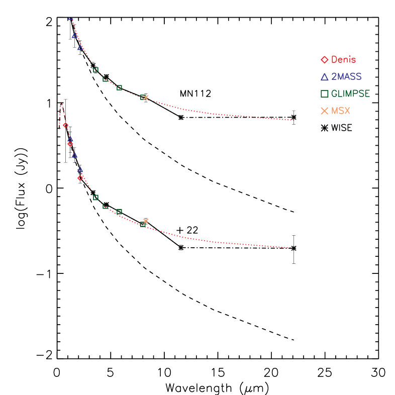
Figure 4: SEDs of star #22 (this work) and of the cLBV MN112 discovered by Gvaramadze et al. (2010). Flux densities in the DENIS, 2MASS, MSX, GLIMPSE, and WISE bands are plotted with diamonds, triangles, squares, crosses, and asterisks, respectively. The WISE 3 (11 $\mu$m) and 4 (20 $\mu$m) measurements were marked as affected by confusion. The long-dashed curves are black-bodies with the stellar effective temperatures. The dotted curves are modified black-bodies, which we created by adding to the continuum a 10-15% of free-free emission ( $\propto\lambda^{-0.6}$), a warm dust component at 650 k, and a cold dust component at 150 k.

The cLBV has been detected as a point-source up to 20 $\mu$m (W4 band of the WISE survey). With a GLIMPSE [3.6]$-$[5.8] = 0.72 mag and a [3.6]$-$[8.0]= 0.96 mag, star #22 well fits in the GLIMPSE color distribution found for known Galactic LBV stars (Messineo et al. 2012). The SED of cLBV #22 resembles that of cLBV MN112 (Gvaramadze et al. 2010), with an excess at several mid-infrared wavelengths (see Fig. 4); however, in contrast to MN112, an extended circumstellar nebulae is not detected. We did not find significant photometric variations in the $J$- and K_s-band of DENIS and 2MASS (Table 6). Nevertheless, high probability of being a variable point source is reported in band $W3$ (11.6 $\mu$m) by the WISE catalog.

Table 6: Near-infrared measurements of cLBV #22.

	DENIS1	DENIS2	2MASS
Date	$22-05-1999$	$29-08-2000$	$29-04-1999$
$I$	$13.88\pm 0.06$	$13.92\pm 0.04$
$J$	$9.70\pm 0.05$	$9.67\pm 0.07$	$9.78\pm 0.02$
$H$	$..$	$..$	$8.42\pm 0.04$
Ks	$7.65\pm 0.06$	$7.51\pm 0.07$	$7.63\pm 0.02$

• Two epochs of DENIS simultaneous $IJ$K_s measurements were available. We re-calibrated the DENIS measurements by using point sources within 1^′; a significant offset was found for epoch one.

3.1.3 Late-type stars

Figure 5: Normalized spectra (arbitrarily shifted for clarity) of detected candidate red supergiants. The spectra were multiplied by the black body of the standard star, and de-reddened. The spectra with shorter coverage were taken with SofI.

The equivalent width of the CO band-head, EW(CO), at 2.29 $\mu$m linearly correlates with the stellar temperature (T_eff). CO absorption also strengthens with increasing luminosity. Therefore, the EW(CO) and T_eff  values of giants and RSGs follow two distinct relations (Blum et al. 2003; Figer et al. 2006; Davies et al. 2007); the sequence of RSGs extends to larger values of EW(CO).

The EWs are based on the Kleinmann & Hall (1986) spectra. We smoothed the reference spectra of Kleinmann & Hall (1986) to the resolution of the observed ones; we de-reddened each target spectrum with the extinction law by Messineo et al. (2005) and the E($J-$K_s) color excess (see Sect. 3.2). The continuum was taken from 2.285 $\mu$m to 2.290 $\mu$m. The EW(CO)s in unit of Angstroms were obtained by integrating the line strength of the CO feature, 1-Flux(CO)/Flux(continuum), in wavelengths (from 2.290 $\mu$m to 2.320 $\mu$m, e.g. Figer et al. 2006). EW(CO)s from medium-resolution spectra taken with SofI were measured in a narrower region, from 2.285 $\mu$m to 2.307 $\mu$m. Typical uncertainties of the estimated spectral-types are within a factor of two, as estimated by slightly shifting the continuum region and the reddening.

Stars with EW(CO)s larger than that of a M7 giant were classified as candidate RSGs or variable AGB stars. A detailed discussion on the identification of AGB stars, which contaminate both red giant and RSG sequences, is provided in Appendix B. After having excluded one AGB star (#56), we found that four other stars show EWs larger that that of an M7III star: #40, #43, #46, and #47.

Spectral types for the 113 detected late-type stars are listed in Tables 3 and 12. Each list is sorted by coordinates. Some spectra of bright late-type stars are displayed in Fig. 5.

3.2 Determination of A${}_{\it K_{\rm s}}$

In the near-infrared, the attenuation of a star’s light by interstellar dust absorption is wavelength-dependent, and may be expressed by a power law $A_{\lambda}$ $\propto\lambda^{-\alpha}$.

For every star, we estimated the effective extinction in K_s-band, A${}_{\it K_{\rm s}}$, by measuring the near-infrared color-excess, and by using $\alpha=-1.9$ (Messineo et al. 2005). We adopted the intrinsic infrared colors per spectral type tabulated by Messineo et al. (2011); they were taken from Martins & Plez (2006) (O-stars in the Bessell system), Wegner (1994) (B-A stars in the Johnson system), Johnson (1966) (B-A dwarfs in the Johnson system), Koornneef (1983) (B-A supergiants and late-types in the Koornneef system), Lejeune & Schaerer (2001) (colors of dwarfs from O3 to A5 in the Bessell system). The used compilation uses data in the Johnson, Bessell, and Koornneef filter systems. Color transformations were not applied, but no significant deviations were found. There is no significant difference between the SAAO and the Johnson system (Carter 1990; Blum et al. 2000). Carpenter (2001) found differences between the SAAO system (or Koornneff system) and the 2mass system well within 0.1 mag. Table 2 lists the adopted intrinsic $(J-K)_{o}$ and $(H-K)_{o}$ colors of early-types.

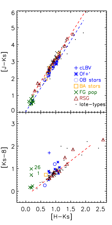
Figure 6: Top panel: the $J-$K_s versus $H-$K_s diagram of the observed stars. Spectral-types are marked as shown in the figure legend; the two dashed curves indicate the reddening curves of naked M1 and O9 stars. Bottom panel: K_s$-8$ versus $H-$K_s diagram; a reddening curve for an M1 star is shown with a dashed line. Star #22 (cLBV) shows infrared excess at 8 $\mu$m. The two foreground stars #1 (OBe) and #26 (B4-A4) have notable infrared excess. Star #7 was not plotted (8 $\mu$m confused).

Figure 7: Histograms of the A${}_{\it K_{\rm s}}$ values for early-type stars (solid line), late-type stars (dotted line), and candidate red supergiants from Table 10 (dashed line).

We assumed as interstellar extinction individual A${}_{\it K_{\rm s}}$ values. For the detected early-type stars, we preferred the total interstellar extinction A${}_{\it K_{\rm s}}$ from the shortest color $E(J-H)$; for late-type stars, we used individual A${}_{\it K_{\rm s}}$ from $J-$K_s (or $H-$K_s) (Koornneef 1983).

A $J-$K_s versus $H-$Ks diagram of the observed sources is shown in Fig. 6. The cLBV displays an infrared excess long-ward of 2 $\mu$m; the O-type stars nicely follow the reddening vectors. The bulk of detected late-type stars (with exclusion of a few AGBs) lacks strong dust excess (Fig. 6), as also inferred from the $Q1$ parameter (see Appendix A).

Figure 7 shows the distribution of A${}_{\it K_{\rm s}}$ for early- and late-type stars. Two distinct populations of early-type stars are found; there is a group of bluer objects with A${}_{\it K_{\rm s}}$$<0.8$ mag, and a group with A${}_{\it K_{\rm s}}$ from 0.9 mag to 2.0 mag. The distribution of A${}_{\it K_{\rm s}}$ of late-type stars peaks around 0.9 mag, and appears unrelated to that of early-types.

At infrared wavelength, Galactic interstellar extinction has been best modeled using a power-law with an index $\alpha$ from $-1.61$ (for example, Rieke & Lebofsky 1985; Indebetouw et al. 2005) to about $-2.1$ (Nishiyama et al. 2006) and Stead & Hoare (2009). For a reddening, E($H-$K_s), of 0.7 and 1.3 mag, $\alpha=-1.9$ yields A${}_{\it K_{\rm s}}$=1 and 2 mag, while $\alpha=-1.61$ would yield A${}_{\it K_{\rm s}}$=1.19 and 2.37 mag, and $\alpha=-2.2$ would yield A${}_{\it K_{\rm s}}$=0.86 and 1.61 mag. Therefore, Rieke’s law would brighten the de-reddened K_s and M_bol of $-0.19$ and $-0.37$ mag; an index of $-2.2$ would dim the de-reddened K_s and M_bol of $+0.14$ and $+0.39$ mag. An index of $-1.9$ provides consistent values of interstellar extinction from multicolor reddenings ( e.g. $E(J-H)$, $E(H-K)$), and $E(J-K)$).

3.3 Spectro-photometric distances

Table 7: Spectrophotometric distances of individual early-type stars.

ID

Kso

A${}_{\it K_{\rm s}}$

Spectral

Class

MK(I)b

MK(III)b

MK(V)b

DM Ia

DM IIIIa

DM Va

Region

[mag]

[mag]

[mag]

[mag]

[mag]

[mag]

[mag]

[mag]

16

7.50

1.68

O9-9.5e

I

-5.39$\pm$ 0.83

-4.47$\pm$ 0.65

-3.30$\pm$ 0.76

12.89 $\pm$ 0.83

11.97 $\pm$ 0.65

10.80 $\pm$ 0.76

REG4

15

7.93

1.59

O6-7fK+

I

-5.28$\pm$ 0.66

-4.84$\pm$ 0.57

-3.99$\pm$ 0.65

13.21 $\pm$ 0.66

12.77 $\pm$ 0.57

11.92 $\pm$ 0.65

GLIMPSE9

36

8.13

1.93

O6-7fK+

I

-5.28$\pm$ 0.66

-4.84$\pm$ 0.57

-3.99$\pm$ 0.65

13.41 $\pm$ 0.66

12.97 $\pm$ 0.57

12.12 $\pm$ 0.65

REG4

4

8.26

1.62

O7-8.5fK+

I

-5.39$\pm$ 0.83

-4.66$\pm$ 0.61

-3.63$\pm$ 0.71

13.65 $\pm$ 1.17

12.92 $\pm$ 1.02

11.89 $\pm$ 1.08

GLIMPSE9

14

8.32

1.86

O6-7fK+

I

-5.28$\pm$ 0.66

-4.84$\pm$ 0.57

-3.99$\pm$ 0.65

13.60 $\pm$ 0.66

13.16 $\pm$ 0.57

12.31 $\pm$ 0.65

GLIMPSE9

18

8.41

1.55

O6-7fK+

I

-5.28$\pm$ 0.66

-4.84$\pm$ 0.57

-3.99$\pm$ 0.65

13.69 $\pm$ 0.66

13.25 $\pm$ 0.57

12.40 $\pm$ 0.65

REG4

25

8.57

1.34

O4fK+

I

-5.16$\pm$ 0.63

-5.05$\pm$ 0.63

-4.41$\pm$ 0.78

13.73 $\pm$ 0.63

13.62 $\pm$ 0.63

12.98 $\pm$ 0.78

REG7

5

8.65

1.73

O6-7fK+

III

-5.28$\pm$ 0.66

-4.84$\pm$ 0.57

-3.99$\pm$ 0.65

13.93 $\pm$ 0.66

13.49 $\pm$ 0.57

12.64 $\pm$ 0.65

GLIMPSE9

9

8.65

1.75

O7-8.5fK+

III

-5.39$\pm$ 0.83

-4.66$\pm$ 0.61

-3.63$\pm$ 0.71

14.04 $\pm$ 0.84

13.31 $\pm$ 0.62

12.28 $\pm$ 0.72

GLIMPSE9

3

8.85

1.90

O6-7fK+

III

-5.28$\pm$ 0.66

-4.84$\pm$ 0.57

-3.99$\pm$ 0.65

14.13 $\pm$ 0.66

13.69 $\pm$ 0.57

12.84 $\pm$ 0.65

GLIMPSE9

23

9.04

1.39

O6-7fK+

III

-5.28$\pm$ 0.66

-4.84$\pm$ 0.57

-3.99$\pm$ 0.65

14.32 $\pm$ 0.66

13.88 $\pm$ 0.57

13.03 $\pm$ 0.65

REG4

17

9.21

1.37

O9-9.5fK+

III

-5.39$\pm$ 0.83

-4.47$\pm$ 0.65

-3.30$\pm$ 0.76

14.60 $\pm$ 0.83

13.68 $\pm$ 0.65

12.51 $\pm$ 0.76

REG4

$[$MFD2010$]$ 3

6.48

1.48

B0-3

I

-6.27$\pm$ 0.92

-3.47$\pm$ 1.43

-2.38$\pm$ 1.27

12.75 $\pm$ 0.97

9.95 $\pm$ 1.46

8.86 $\pm$ 1.30

GLIMPSE9

$[$MFD2010$]$ 4

7.48

1.66

B0-3

I

-6.27$\pm$ 0.92

-3.47$\pm$ 1.43

-2.38$\pm$ 1.27

13.75 $\pm$ 0.92

10.95 $\pm$ 1.43

9.86 $\pm$ 1.27

GLIMPSE9

6

9.02

1.51

B0-3

III

-6.49$\pm$ 1.14

-3.47$\pm$ 1.43

-2.38$\pm$ 1.27

15.51 $\pm$ 1.15

12.49 $\pm$ 1.43

11.40 $\pm$ 1.27

GLIMPSE9

31

9.05

1.26

B0-3

III

-6.49$\pm$ 1.14

-3.47$\pm$ 1.43

-2.38$\pm$ 1.27

15.54 $\pm$ 1.14

12.52 $\pm$ 1.43

11.43 $\pm$ 1.27

REG2

38

9.37

1.13

B0-3

III

-6.49$\pm$ 1.14

-3.47$\pm$ 1.43

-2.38$\pm$ 1.27

15.86 $\pm$ 1.14

12.84 $\pm$ 1.43

11.75 $\pm$ 1.27

REG4

21

9.64

1.11

B7.5-A2

III

-7.04$\pm$ 0.65

$..$

-0.41$\pm$ 1.25

16.68 $\pm$ 0.65

$..$

10.05 $\pm$ 1.25

REG4

8

10.34

1.67

B0-3

III

-6.49$\pm$ 1.14

-3.47$\pm$ 1.43

-2.38$\pm$ 1.27

16.83 $\pm$ 1.14

13.81 $\pm$ 1.43

12.72 $\pm$ 1.27

GLIMPSE9

2

6.10

0.51

O9-9.5e

I

-5.39$\pm$ 0.83

-4.47$\pm$ 0.65

-3.30$\pm$ 0.76

11.49 $\pm$ 0.83

10.57 $\pm$ 0.65

9.40 $\pm$ 0.76

$..$

19

9.94

0.42

B4-A2

V

-7.04$\pm$ 0.65

$..$

-0.41$\pm$ 1.25

16.98 $\pm$ 0.65

$..$

10.35 $\pm$ 1.25

REG5

12

10.07

0.32

B4-A2

V

-7.04$\pm$ 0.65

$..$

-0.41$\pm$ 1.25

17.11 $\pm$ 0.65

$..$

10.48 $\pm$ 1.25

REG5

13

10.08

0.29

B4-A2

V

-7.04$\pm$ 0.65

$..$

-0.41$\pm$ 1.25

17.12 $\pm$ 0.65

$..$

10.49 $\pm$ 1.25

REG5

32

10.19

0.37

B4-A2

V

-7.04$\pm$ 0.65

$..$

-0.41$\pm$ 1.25

17.23 $\pm$ 0.65

$..$

10.60 $\pm$ 1.25

REG5

26

10.42

0.31

B4-A2

V

-7.04$\pm$ 0.65

$..$

-0.41$\pm$ 1.25

17.46 $\pm$ 0.65

$..$

10.83 $\pm$ 1.25

REG5

28

10.48

0.30

B4-A2

V

-7.04$\pm$ 0.65

$..$

-0.41$\pm$ 1.25

17.52 $\pm$ 0.65

$..$

10.89 $\pm$ 1.25

REG5

7

10.54

0.42

B4-A2

V

-7.04$\pm$ 0.65

$..$

-0.41$\pm$ 1.25

17.58 $\pm$ 0.65

$..$

10.95 $\pm$ 1.25

REG5

20

11.95

0.47

B4-A2

V

-7.04$\pm$ 0.65

$..$

-0.41$\pm$ 1.25

18.99 $\pm$ 0.65

$..$

12.36 $\pm$ 1.25

REG4

• Notes. Identification numbers from Table 2 are followed by de-reddened K_s, (K_so), A${}_{\it K_{\rm s}}$, spectral types, estimated luminosity classes, absolute magnitudes in the K_s-band for class I, III, V, distances, and regions. The table lists O-type stars with A${}_{\it K_{\rm s}}$$>0.8$ mag, then B-stars with A${}_{\it K_{\rm s}}$$>0.8$ mag, and finally star with A${}_{\it K_{\rm s}}$$<0.8$ mag.  Each block is ordered by de-reddened K_s.  (^a) Distance modulus for the estimated luminosity classes are marked in bold (see text).  (^b) Quoted errors on M_K are calculated by assuming an error of 0.5 mag on a single type (e.g. Bibby et al. 2008; Humphreys & McElroy 1984). Note that the quoted M_K values are used to derive spectrophotometric DMs. Later, in Table 9, we will assume a common distance and recalculate M_K and M_bol.

Table 8: Average spectro-photometric distance of stars with A${}_{\it K_{\rm s}}$$>$0.8 mag.

Spec.	Lum Class	Nstar	$<$A${}_{\it K_{\rm s}}$$>$	MK	$<$DM$>$	REF.
			[mag]	[mag]	[mag]
O4-6	I	1	1.34	-5.16	13.73$\pm$ 0.63	1,2
O6-7	I	4	1.73	-5.28	13.48$\pm$ 0.21	1,2,3
O7-8.5	I	1	1.62	-5.39	13.65$\pm$ 1.17	3
O9-9.5	I	1	1.68	-5.39	12.89$\pm$ 0.83	3
O6-7	III	3	1.67	-4.84	13.69$\pm$ 0.20	4
O7-8.5	III	1	1.75	-4.66	13.31$\pm$ 0.62	4
O9-9.5	III	1	1.37	-4.47	13.68$\pm$ 0.65	4
B0-3	I	2	1.57	-6.27	13.25$\pm$ 0.71	5

• Notes. Classes were assigned by assuming similar distances; only supergiants yielded independent estimates. For each group (see Table 7 ) and luminosity class, we report the number of stars (Nstars), average A${}_{\it K_{\rm s}}$, average distance modulus, and standard deviation.

• References. (1) Figer et al. (2002);  (2) Martins et al. (2008);  (3) Messineo et al. (2011);  (4) Martins & Plez (2006);  (5) Bibby et al. (2008).

Table 9: List of estimated stellar parameters for the sample of early-type stars with A${}_{\it K_{\rm s}}$$>0.8$ mag.

ID	Sp. Type	Kso	A${}_{\it K_{\rm s}}$($JH$)	A${}_{\it K_{\rm s}}$($J$Ks)	A${}_{\it K_{\rm s}}$($H$Ks)	$Q1$	BC${}_{\it K_{\mathrm{s}}}$	DM	Mbol
		[mag]	[mag]	[mag]	[mag]	[mag]	[mag]	[mag]	[mag]
3	O6$-$7fK+	8.85 $\pm$ 0.04	1.90 $\pm$ 0.03	1.86 $\pm$ 0.02	1.79 $\pm$ 0.05	0.19 $\pm$ 0.08	$-$4.28 $\pm$ 0.09	13.31 $\pm$ 0.17	$-$8.74$\pm$ 0.20
4	O7$-$8.5fK+	8.26 $\pm$ 0.82	1.62 $\pm$ 0.20	1.64 $\pm$ 0.20	1.69 $\pm$ 0.20	$-$0.03 $\pm$ 0.80	$-$3.97 $\pm$ 0.12	13.31 $\pm$ 0.17	$-$9.02$\pm$ 0.85
5	O6$-$7fK+	8.65 $\pm$ 0.04	1.73 $\pm$ 0.03	1.68 $\pm$ 0.02	1.60 $\pm$ 0.05	0.20 $\pm$ 0.08	$-$4.28 $\pm$ 0.09	13.31 $\pm$ 0.17	$-$8.94$\pm$ 0.20
6	B0$-$3	9.02 $\pm$ 0.11	1.51 $\pm$ 0.10	1.49 $\pm$ 0.07	1.46 $\pm$ 0.04	0.11 $\pm$ 0.14	$-$2.83 $\pm$ 0.87	13.31 $\pm$ 0.17	$-$7.11$\pm$ 0.89
8	B0$-$3	10.34 $\pm$ 0.00	1.67 $\pm$ 0.00	1.65 $\pm$ 0.00	1.62 $\pm$ 0.00	0.11 $\pm$ 0.00	$-$2.83 $\pm$ 0.87	13.31 $\pm$ 0.17	$-$5.80$\pm$ 0.89
9	O7$-$8.5fK+	8.65 $\pm$ 0.11	1.75 $\pm$ 0.06	1.74 $\pm$ 0.05	1.71 $\pm$ 0.16	0.11 $\pm$ 0.23	$-$4.05 $\pm$ 0.14	13.31 $\pm$ 0.17	$-$8.71$\pm$ 0.25
14	O6$-$7fK+	8.32 $\pm$ 0.04	1.86 $\pm$ 0.04	1.82 $\pm$ 0.02	1.75 $\pm$ 0.05	0.18 $\pm$ 0.10	$-$4.17 $\pm$ 0.08	13.31 $\pm$ 0.17	$-$9.16$\pm$ 0.19
15	O6$-$7fK+	7.93 $\pm$ 0.04	1.59 $\pm$ 0.03	1.56 $\pm$ 0.02	1.50 $\pm$ 0.05	0.17 $\pm$ 0.09	$-$4.17 $\pm$ 0.08	13.31 $\pm$ 0.17	$-$9.55$\pm$ 0.19
16	O9$-$9.5e	7.50 $\pm$ 0.04	1.68 $\pm$ 0.03	1.64 $\pm$ 0.02	1.55 $\pm$ 0.05	0.18 $\pm$ 0.08	$-$3.62 $\pm$ 0.32	13.31 $\pm$ 0.17	$-$9.43$\pm$ 0.36
17	O9$-$9.5fK+	9.21 $\pm$ 0.04	1.37 $\pm$ 0.03	1.35 $\pm$ 0.02	1.32 $\pm$ 0.06	0.11 $\pm$ 0.10	$-$3.80 $\pm$ 0.21	13.31 $\pm$ 0.17	$-$7.90$\pm$ 0.27
18	O6$-$7fK+	8.41 $\pm$ 0.03	1.55 $\pm$ 0.03	1.46 $\pm$ 0.02	1.29 $\pm$ 0.04	0.36 $\pm$ 0.07	$-$4.17 $\pm$ 0.08	13.31 $\pm$ 0.17	$-$9.07$\pm$ 0.19
21	B7.5$-$A2	9.64 $\pm$ 0.04	1.11 $\pm$ 0.03	1.07 $\pm$ 0.02	1.00 $\pm$ 0.05	0.11 $\pm$ 0.08	$-$0.92 $\pm$ 0.92	13.31 $\pm$ 0.17	$-$4.59$\pm$ 0.94
22	cLBV	6.50 $\pm$ 0.05	1.13 $\pm$ 0.04	1.15 $\pm$ 0.02	1.19 $\pm$ 0.08	$-$0.04 $\pm$ 0.14	$-$1.09 $\pm$ 0.62	13.31 $\pm$ 0.17	$-$7.90$\pm$ 0.64
23	O6$-$7fK+	9.04 $\pm$ 0.04	1.39 $\pm$ 0.03	1.36 $\pm$ 0.02	1.30 $\pm$ 0.05	0.17 $\pm$ 0.09	$-$4.28 $\pm$ 0.09	13.31 $\pm$ 0.17	$-$8.55$\pm$ 0.20
25	O4fK+	8.57 $\pm$ 0.04	1.34 $\pm$ 0.03	1.32 $\pm$ 0.02	1.30 $\pm$ 0.05	0.10 $\pm$ 0.09	$-$4.40 $\pm$ 0.15	13.31 $\pm$ 0.17	$-$9.14$\pm$ 0.23
31	B0$-$3	9.05 $\pm$ 0.06	1.26 $\pm$ 0.05	1.26 $\pm$ 0.03	1.24 $\pm$ 0.08	0.08 $\pm$ 0.15	$-$2.83 $\pm$ 0.87	13.31 $\pm$ 0.17	$-$7.09$\pm$ 0.89
36	O6$-$7fK+	8.13 $\pm$ 0.04	1.93 $\pm$ 0.03	1.90 $\pm$ 0.02	1.84 $\pm$ 0.05	0.16 $\pm$ 0.09	$-$4.17 $\pm$ 0.08	13.31 $\pm$ 0.17	$-$9.35$\pm$ 0.19
38	B0$-$3	9.37 $\pm$ 0.04	1.13 $\pm$ 0.03	1.11 $\pm$ 0.02	1.07 $\pm$ 0.05	0.13 $\pm$ 0.08	$-$2.83 $\pm$ 0.87	13.31 $\pm$ 0.17	$-$6.77$\pm$ 0.89
$[$MFD2010$]$ 3	B0$-$3	6.48 $\pm$ 0.30	1.48 $\pm$ 0.03	1.49 $\pm$ 0.16	1.51 $\pm$ 0.45	$-$0.02 $\pm$ 0.54	$-$2.50 $\pm$ 0.80	13.31 $\pm$ 0.17	$-$9.33$\pm$ 0.87
$[$MFD2010$]$ 4	B0$-$3	7.48 $\pm$ 0.05	$..$	$..$	1.66 $\pm$ 0.04	$..$	$-$2.50 $\pm$ 0.80	13.31 $\pm$ 0.17	$-$8.33$\pm$ 0.82
WR 39	WC8	8.01 $\pm$ 0.03	1.35 $\pm$ 0.03	1.28 $\pm$ 0.02	1.17 $\pm$ 0.05	$-$0.44 $\pm$ 0.08	$-$3.60 $\pm$ 0.50	13.31 $\pm$ 0.17	$-$8.90$\pm$ 0.53
1	OBe	8.86 $\pm$ 0.04	0.31 $\pm$ 0.03	0.33 $\pm$ 0.02	0.36 $\pm$ 0.05	$-$0.02 $\pm$ 0.08	$-$2.87 $\pm$ 1.21	12.39 $\pm$ 1.00	$-$6.40$\pm$ 1.57
2	O9$-$9.5e	6.10 $\pm$ 0.04	0.51 $\pm$ 0.03	0.48 $\pm$ 0.02	0.44 $\pm$ 0.05	0.12 $\pm$ 0.09	$-$3.62 $\pm$ 0.32	12.39 $\pm$ 1.00	$-$9.90$\pm$ 1.05
7	B4$-$A2	10.54 $\pm$ 0.04	0.42 $\pm$ 0.03	0.41 $\pm$ 0.02	0.39 $\pm$ 0.05	0.02 $\pm$ 0.09	$-$0.99 $\pm$ 0.96	12.39 $\pm$ 1.00	$-$2.84$\pm$ 1.39
12	B4$-$A2	10.07 $\pm$ 0.05	0.32 $\pm$ 0.04	0.30 $\pm$ 0.02	0.28 $\pm$ 0.07	0.02 $\pm$ 0.12	$-$0.99 $\pm$ 0.96	12.39 $\pm$ 1.00	$-$3.31$\pm$ 1.39
13	B4$-$A2	10.08 $\pm$ 0.04	0.29 $\pm$ 0.03	0.26 $\pm$ 0.02	0.20 $\pm$ 0.05	0.08 $\pm$ 0.08	$-$0.99 $\pm$ 0.96	12.39 $\pm$ 1.00	$-$3.29$\pm$ 1.39
19	B4$-$A2	9.94 $\pm$ 0.04	0.42 $\pm$ 0.03	0.39 $\pm$ 0.02	0.34 $\pm$ 0.05	0.07 $\pm$ 0.08	$-$0.99 $\pm$ 0.96	12.39 $\pm$ 1.00	$-$3.44$\pm$ 1.39
20	B4$-$A2	11.95 $\pm$ 0.00	0.47 $\pm$ 0.00	0.35 $\pm$ 0.00	0.15 $\pm$ 0.00	0.35 $\pm$ 0.00	$-$0.99 $\pm$ 0.96	12.39 $\pm$ 1.00	$-$1.42$\pm$ 1.39
26	B4$-$A2	10.42 $\pm$ 0.04	0.31 $\pm$ 0.03	0.30 $\pm$ 0.02	0.27 $\pm$ 0.05	0.02 $\pm$ 0.08	$-$0.99 $\pm$ 0.96	12.39 $\pm$ 1.00	$-$2.95$\pm$ 1.39
28	B4$-$A2	10.48 $\pm$ 0.04	0.30 $\pm$ 0.03	0.33 $\pm$ 0.02	0.39 $\pm$ 0.06	$-$0.12 $\pm$ 0.10	$-$0.99 $\pm$ 0.96	12.39 $\pm$ 1.00	$-$2.90$\pm$ 1.39
32	B4$-$A2	10.19 $\pm$ 0.05	0.37 $\pm$ 0.03	0.36 $\pm$ 0.02	0.34 $\pm$ 0.07	0.02 $\pm$ 0.10	$-$0.99 $\pm$ 0.96	12.39 $\pm$ 1.00	$-$3.18$\pm$ 1.39

• Notes. Identification numbers, which are taken from Table 2, are followed by spectral types, de-reddened K_s magnitudes, three estimates of total extinction (A${}_{\it K_{\rm s}}$(JH), A${}_{\it K_{\rm s}}$(JK),A${}_{\it K_{\rm s}}$(HKs)), $Q1$, BC${}_{\it K_{\mathrm{s}}}$, DM, and bolometric magnitudes, M_bol.  Errors in A${}_{\it K_{\rm s}}$($JH$), A${}_{\it K_{\rm s}}$($J$K_s), and A${}_{\it K_{\rm s}}$($H$K_s) values were obtained by propagating the photometric errors of the two considered bands; missing A${}_{\it K_{\rm s}}$ errors were filled with 0.2 mag (star #4). Errors in M_bol were derived by propagation of the errors in K_s magnitudes, A${}_{\it K_{\rm s}}$, BC${}_{\it K_{\mathrm{s}}}$, and DM. Errors in $Q1$ were derived by propagating the errors in $JH$K_s; missing errors in K_s (star #4) were filled with 0.80 mag.

Table 10: Photometric properties of detected candidate RSGs (luminosity L $>10^{4}$ L_⊙, masses $>9$ M_⊙).

IDa	$(J-K_{\rm s})$o	$(H-K_{\rm s})$o	A${}_{\it K_{\rm s}}$($J$Ks)b	A${}_{\it K_{\rm s}}$($H$Ks)b	$Q1$b	Ksob	BC${}_{\it K_{\rm s}}$	DM	Mbol[mag]e	Com.	region
	[mag]	[mag]	[mag]	[mag]	[mag]	[mag]		[mag]	[mag]
39	0.96	0.20	0.84 $\pm$ 0.02	0.87 $\pm$ 0.06	0.33 $\pm$ 0.09	4.00 $\pm$ 0.03	2.64	13.31 $\pm$ 0.17	$-$6.67 $\pm$ 0.53
40	0.99	0.21	1.95 $\pm$ 0.02	2.04 $\pm$ 0.07	0.22 $\pm$ 0.12	3.12 $\pm$ 0.03	2.70	13.31 $\pm$ 0.17	$-$7.49 $\pm$ 0.53	RSGf	rsgcx1
41	0.72	0.15	1.27 $\pm$ 0.02	1.17 $\pm$ 0.07	0.47 $\pm$ 0.12	5.25 $\pm$ 0.03	2.55	13.31 $\pm$ 0.17	$-$5.51 $\pm$ 0.53		rsgcx1
42	0.72	0.15	1.03 $\pm$ 0.02	0.95 $\pm$ 0.06	0.44 $\pm$ 0.11	5.11 $\pm$ 0.03	2.55	13.31 $\pm$ 0.17	$-$5.65 $\pm$ 0.53		rsgcx1
43	0.99	0.21	$..$	3.54 $\pm$ 0.06	$..$	4.36 $\pm$ 0.06	2.70	13.31 $\pm$ 0.17	$-$6.25 $\pm$ 0.53	RSG
44	0.62	0.13	1.20 $\pm$ 0.02	1.13 $\pm$ 0.07	0.36 $\pm$ 0.12	4.64 $\pm$ 0.03	2.50	13.31 $\pm$ 0.17	$-$6.17 $\pm$ 0.53
45	0.72	0.15	1.33 $\pm$ 0.02	1.33 $\pm$ 0.07	0.29 $\pm$ 0.13	4.88 $\pm$ 0.03	2.55	13.31 $\pm$ 0.17	$-$5.88 $\pm$ 0.53
46	1.16	0.28	1.49 $\pm$ 0.02	1.53 $\pm$ 0.08	0.27 $\pm$ 0.14	4.80 $\pm$ 0.03	2.84	13.31 $\pm$ 0.17	$-$5.67 $\pm$ 0.53	RSG	glimpse9
47	1.06	0.25	1.26 $\pm$ 0.02	1.31 $\pm$ 0.06	0.24 $\pm$ 0.11	4.93 $\pm$ 0.03	2.80	13.31 $\pm$ 0.17	$-$5.58 $\pm$ 0.53	RSG	reg4
48	0.96	0.20	1.08 $\pm$ 0.02	1.10 $\pm$ 0.06	0.35 $\pm$ 0.09	4.98 $\pm$ 0.03	2.64	13.31 $\pm$ 0.17	$-$5.69 $\pm$ 0.53		reg4
$[$MFD2010$]$ 5	1.03	0.23	1.79 $\pm$ 0.02	1.71 $\pm$ 0.06	0.50 $\pm$ 0.10	5.26 $\pm$ 0.04	2.76	13.31 $\pm$ 0.17	$-$5.29 $\pm$ 0.53	RSG	glimpse9
BD$-$08 4635	1.06	0.25	0.36 $\pm$ 0.19	0.22 $\pm$ 0.51	0.63 $\pm$ 0.81	2.69 $\pm$ 0.32	2.80	12.39 $\pm$ 0.50	$-$6.90 $\pm$ 0.78		reg2
BD$-$08 4639	0.62	0.13	0.36 $\pm$ 0.17	0.24 $\pm$ 0.42	0.46 $\pm$ 0.68	2.41 $\pm$ 0.27	2.50	12.39 $\pm$ 0.50	$-$7.48 $\pm$ 0.76
BD$-$08 4645	1.06	0.25	0.31 $\pm$ 0.15	0.28 $\pm$ 0.39	0.40 $\pm$ 0.65	1.99 $\pm$ 0.24	2.80	12.39 $\pm$ 0.50	$-$7.60 $\pm$ 0.75	RSG

• Notes. Identification numbers, are followed by intrinsic $(J-K_{\rm s})$_o , $(H-K_{\rm s})$_o colors, A${}_{\it K_{\rm s}}$($J$K_s) and A${}_{\it K_{\rm s}}$($H$K_s), $Q1$ , de-reddened K_s, K_so, and absolute bolometric magnitudes.   (^a) Identification numbers are taken from Table 3.  (^b) Errors in A${}_{\it K_{\rm s}}$, K_so, $Q1$, M_bol  are calculated by propagation of the photometric errors.  (^e) M_bol is obtained with the BC${}_{\it K_{\mathrm{s}}}$ of Levesque et al. (2005).  (^f) The RSG comment denotes known RSGs ( MFD2010 5 and BD$-$08 4645, e.g.  Sylvester et al. 1998; Messineo et al. 2010), and stars #40, #43, #46, and #47, which have EW(CO)s larger than that of a M7III, typical of M0-2I.

The distance modulus $DM$ is by definition equal to

$$DM=K_{\mathrm{s}}-A_{\it K_{\mathrm{s}}}-M_{\it K},$$

where A${}_{\it K_{\rm s}}$ is the extinction and $M_{\it K}$ is the absolute magnitude in $K$-band; A${}_{\it K_{\rm s}}$ and $M_{\it K}$ are function of spectral types and luminosity classes. Early-type stars with known spectral-types yield spectro-photometric distances, when assumptions on luminosity classes can be made, and erratic behaviors are not present (e.g. LBVs). Compilations of absolute $K$ magnitudes and intrinsic colors for O and B types are available from Johnson (1966), Koornneef (1983), Humphreys & McElroy (1984), Wegner (1994), Lejeune & Schaerer (2001), Crowther et al. (2006), and Martins & Plez (2006). In the near-infrared, spectral classification can be achieved to within a few classes (Hanson et al. 1996), and a range of $M_{\it K}$ must be assumed; for a O4-6 star, for example, we assumed the average $M_{\it K}$ of those of O4 and O6 stars. For each star, $M_{\it K}$ and DM were estimated for the dwarf, giant, and supergiant classes, as summarized in Tables 7 and 8. We assumed that stars at similar interstellar extinction were likely to be at similar distances; we calculated the DMs of a few detected spectroscopic supergiants; we assigned luminosities classes to fainter stars by comparing their A${}_{\it K_{\rm s}}$ and K_s to those of supergiants of the same spectral type.

O-type stars have $1.3\la$ A${}_{\it K_{\rm s}}$$\la 1.9$ mag. Stars #14, #16, and #25 are O-type supergiants, as suggested by their emission lines (Hanson et al. 1996, 2005) – a strong He I line at 2.058 $\mu$m appear in emission in the spectrum of star #16; a broad line emission at 2.115 $\mu$m (typical of f-type and WR stars) and strong C IV emission lines are seen in star #25; star #14 has strong He I lines in absorption, but Br_γ in emission. There are four O-type stars with K_s magnitudes brighter than those of stars #14, #16, and #25; for those we assumed a supergiant class.

Absolute magnitudes of O-types are, however, quite uncertain. The Arches cluster is rich in O4–6 stars, and is located at the distance of the Galactic center (Martins et al. 2008). We recalculated an average value of $M_{\it K}=-4.94\pm 0.47$ mag for all O4–6I stars in the Arches listed by Martins et al. (2008) (hyper-giants F10 and F15 were included), and of $-5.16\pm 0.13$ mag for those O4–6I with He I line at 2.112 $\mu$m in absorption; we used 8.4 kpc, the photometry from Figer et al. (2002) and the extinction law by Messineo et al. (2005). The O7–9I stars in W33 yield $M_{\it K}=-5.39\pm 0.33$ mag. All, but one, Of_K+ stars in GMC G23.3$-$0.3 have the He I line at 2.112 $\mu$m in absorption, and mostly weak carbon lines (O6-7). This empirical comparison implies DM from $13.3\pm 0.4$ mag to $13.5\pm 0.4$ mag for the newly detected OIf_K+ stars. Beside the OIf_K+ stars, we detected only another OI star (O9-9.5, #16), which yields a distance of $4.3^{+1.5}_{-1.1}$ kpc (DM=$13.18\pm 0.66$ mag) by assuming $M_{\it K}=-5.68$ mag.

The two B-type supergiants (A${}_{\it K_{\rm s}}$=1.5 mag) yield a spectrophotometric distance of 4.9 kpc (DM=13.47 mag), when assuming a O9.5-B5 type ($M_{\it K}=-6.49$ mag ), or of 4.5 kpc (DM=13.25 mag), when assuming the more frequently observed O9.5-B3 type ($M_{\it K}=-6.27$ mag). The results from each group and luminosity class are summarized in Table 8.

The derived distance moduli indicate that the OI and BI are consistent with a unique distance. By averaging the distance modulus obtained for BI stars and that for OI stars with M_K from Martins & Plez (2006), we obtained DM=13.48$\pm$0.32 mag; by using the empirical calibration on the Arches, we obtained DM=$13.35\pm 0.14$ mag. For the remaining O-types, since distances increase with decreasing K_so, a mix of luminosity classes (giants and dwarfs) is inferred by assuming similar distances.

Previous studies of H II regions or SNRs (e.g. W41) of this molecular complex report gasous kinematic distances from 4 to 5 kpc (e.g.  Albert et al. 2006; Leahy & Tian 2008). Gas measurements in the direction of the GMC are found to peak at a velocity from $70.5$ to $82.5$ km s^-1 (Messineo et al. 2010, and reference therein); using these velocities and the Galactic curve (R${}_{0}=8.4$ kpc and $\Theta_{0}=254$ km s^-1) from Reid et al. (2009), we obtained a kinematic distance from 4.35 kpc to 4.78 kpc (DM from 13.19 mag to 13.39 mag); by using the historical curve of Brand & Blitz (1993) (R${}_{0}=8.5$ kpc and $\Theta_{0}=220$ km s^-1), we obtained a kinematic distance from 4.6 kpc to 5.1 kpc (DM from 13.31 mag to 13.53 mag). Brunthaler et al. (2009) provides a parallactic distance of $4.59^{+0.38}_{-0.33}$ kpc (DM=13.31$\pm$0.17 mag) for G23.01$-$0.41.

The inferred spectrophotometric distances of O- and B-type supergiants are within the errors consistent with those of the GMC G23.3$-$0.3; these stars are most likely associated with the GMC. Fainter O stars are likely to be giant stars of the same GMC, as supported by their A${}_{\it K_{\rm s}}$ values.

The spectrophotometric distances agree well within errors with the kinematic distance of the cloud and parallactic distance. In the following, the photometric properties of stars associated with the GMC are analyzed by assuming the parallactic distance by Brunthaler et al. (2009).

For the foreground B4-A2 stars, we derived a distance modulus of DM=$10.87\pm 0.64$ mag by assuming a dwarf class.

3.4 Luminosities

Bolometric magnitudes, M_bol, were derived using K_s magnitudes, A${}_{\it K_{\rm s}}$  (see Section 3.2), bolometric corrections, BC${}_{\it K_{\mathrm{s}}}$, effective temperatures, and distance moduli:

$M_{\mathrm{b}ol}=K_{\mathrm{s}}-A_{K_{\mathrm{s}}}+BC_{K_{\mathrm{s}}}+DM.$

For early-type stars, assumed effective temperatures and BC${}_{\it K_{\mathrm{s}}}$ are listed in Tables 2 and 9 (see also Appendix A in Messineo et al. 2011, and references therein); for late type stars, BC${}_{\it K_{\mathrm{s}}}$ and T_eff were available from the work of Levesque et al. (2005). Luminosity properties are discussed only for stars with A${}_{\it K_{\rm s}}$$>0.8$ mag, for which a DM of $13.31\pm 0.17$ mag is assumed.

The luminosities of early-types with emission lines (#14, #16, #22, and #25) range from $1.0\times 10^{5}$ L_⊙  to $4.6\times 10^{5}$ L_⊙, and are consistent with those of blue supergiants. Eleven out of 21 stars with A${}_{\it K_{\rm s}}$$>0.8$ mag are blue supergiants (including [MFD2010]3 and [MFD2010]4 and [MVM2011] 39), ten others are most likely giants; for the Magellanic clouds, Humphreys & McElroy (1984) estimated 7 blue giants for every 10 blue supergiants in both associations and fields.

We selected as candidate RSGs those observed late-type stars with A${}_{\it K_{\rm s}}$$>0.8$ mag and with luminosities larger than $>10^{4}$ L_⊙ for a distance of 4.6 kpc (stars from #39 to #48 in Table 10); star (#46) is a known RSG (Messineo et al. 2010)); contaminating AGB stars were identified by their strong water absorption, as described in Appendix B. The two RSGs in the cluster GLIMPSE9 ( $[$MFD2010$]$5 and #46/$[$MFD2010$]$8 ) have an average A${}_{\it K_{\rm s}}$=1.6 mag, an average M_bol= 5.48 mag (4.6 kpc) and M1.5-3 types (Messineo et al. 2010). The new RSGs, #40 and #47, have types M0I and M2I, A_K= 2.0 and 1.3 mag, and M_bol $-7.49$ mag and $=-5.58$, respectively; they are consistent with the distance of GLIMPSE9 and the GMC. The RSG #43 is a luminous and distant object with A${}_{\it K_{\rm s}}$= 3.5 mag, negligible water absorption, and a large EW(CO). For completeness, Table 10 comprises also stars #39, #41, #42, #44, #45, and #48, which, however, have a slightly lower A${}_{\it K_{\rm s}}$ (1.1 mag) and earlier spectral types (K2-K5). Studies of stellar velocities may provide evidence for a cluster of stars.

3.5 Spatial distribution of massive stars

In Figure 8, the positions of early-type stars and candidate RSG stars are plotted on a grey scale image of the GMC complex at 3.6 $\mu$m by GLIMPSE. In the following sections, the properties of the detected massive stars across several regions of the cloud (see Table 1) are described.

3.6 GLIMPSE9Large

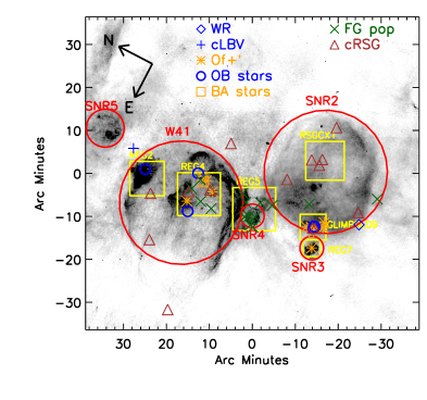
Figure 8: Positions of detected stars are marked on a gray scale, which is a MAGPIS image at 20 cm of the whole G$23.3-0.3$ complex (White et al. 2005; Helfand et al. 2006). Positions of Of${}_{K}^{+}$ stars are marked with asterisks, the cLBV with a plus sign, the WR found by Mauerhan et al. (2011) with a diamond, late-O and early-B types with circles, late-B and early-A stars with squares, and RSGs and cRSGs with triangles. Possible foreground early-types ( A${}_{\it K_{\rm s}}$$<0.8$ mag) are marked with crosses. Locations and sizes of supernova remnants (SNRs) are marked by circles. Squares and labels display the regions selected on the GLIMPSE 3.6 $\mu$m by Messineo et al. (2010) with increased nebular emission (Hii regions) and apparent overdensities of bright stars.

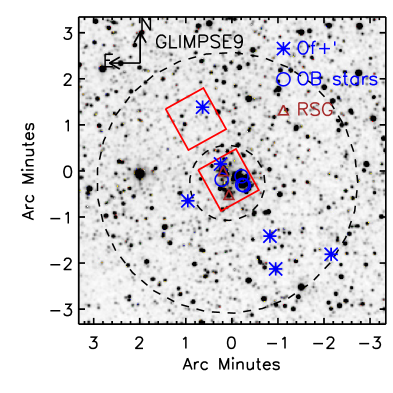
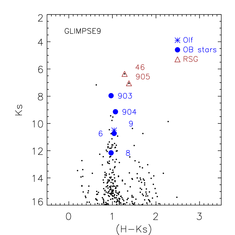
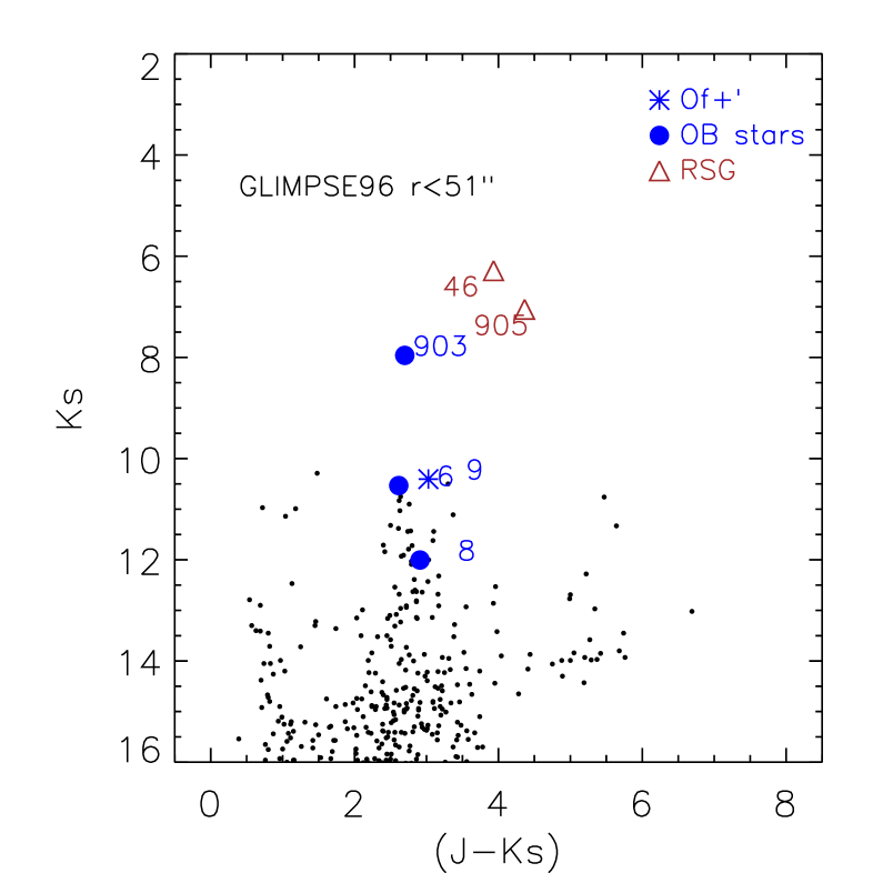
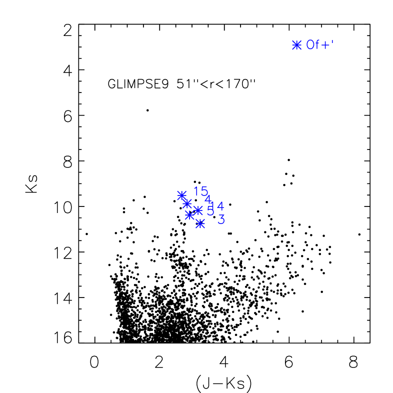
Figure 9: Left upper panel: 2MASS K_s-band image of the observed region GLIMPSE9Large in Table 1. The enclosed NICMOS ($51\hbox to0.0pt{.\hss}^{\prime\prime}5\times 51$^′′) fields studied by Messineo et al. (2010) are shown as squares; the central NICMOS field covers the stellar cluster GLIMPSE9. Two dashed circles indicate the circle and annular regions used for the CMDs. Upper right panel: HST/NICMOS $H-$K_s vs K_s diagram of the GLIMPSE9 cluster (Messineo et al. 2010). Left lower panel: UKIDSS-2MASS K_s versus $J-$K_s diagram of the GLIMPSE9 cluster (2MASS data are used above K_s$\approx 10.5$ mag). Right lower panel: UKIDSS-2MASS K_s versus $J-$K_s diagram of a region surrounding the GLIMPSE9 cluster. Spectroscopically observed stars are marked as summarized in the legend. Of${}_{K}^{+}$ stars are marked with asterisks, late-O and early-B types with filled circles, RSGs and cRSGs with triangles. Labels 903, 904, 905 indicate massive stars [MFD2010]3, [MFD2010]4, and [MFD2010]5 from Messineo et al. (2010).

The surveyed region GLIMPSE9Large has a diameter 7 times larger than the NICMOS field studied by Messineo et al. (2010), as shown in Figs. 8, and 9. Only one Of_K+ star lies in the NICMOS field. A surprisingly large number of massive Of_K+ stars (#3, #4, #5, #9, #14, and #15) are found to surround the GLIMPSE9 cluster. UKIDSS/2MASS K_s versus $J-$K_s diagrams of this region are shown in Fig. 9. Most of the bright stars in the populous diagram of the lower right panel are late-type stars; indeed, a sequence made of clump stars is recognizable, which runs from $J-$K_s$\approx 1$ mag and K_s=11 mag to $J-$K_s$\approx 5$ mag and K_s=14.5 mag; there is a tail of obscured giants stars ($J-$K_s$>4$ mag), and a blue main sequence appears at $J-$K_s$\approx 1$ mag and K_s= 12-16 mag. Detected massive Of_K+ stars have colors similar to those of the GLIMPSE9 cluster, $J-$K_s$\approx 3$ mag, and K_s from 9.52 to 10.75 mag.

The central concentration, i.e. the stellar cluster GLIMPSE9, hosts two RSGs and two B0-3 supergiants (Messineo et al. 2010). The RSG members ([MFD2010]5 and #46/[MFD2010]8) have A${}_{\it K_{\rm s}}$ from 1.49 to 1.79 mag, and M_bol  from $-$5.67 to $-$5.29 mag (for 4.6 kpc), respectively.

The Of_K+ stars are not concentrated, but sparse on a 6^′ radius area (8.0 pc at 4.6 kpc). Their A${}_{\it K_{\rm s}}$ range from 1.59 mag to 1.90 mag. The infrared magnitudes of the Of_K+ stars are consistent with a distance of 4.6 kpc, and with their association with GMC G23.3$-$0.3; their M_bol range from $-$9.55 to $-$8.70 mag; stars #4, #14, and #15 (Of_K+) are supergiants.

3.7 REG4

An overdensity of bright stars on a nebular background, which extends for about 6^′, was visually detected in REG4 (Figs.  1, 8) by Messineo et al. (2010). Four Of_K+ stars, 2 B-type stars, 1 RSG, and 1 cRSG were detected in region REG4. The minimum circle enclosing the four Of_K+ has a diameter of 7^′.

The CMD of region REG4 shows (see Fig. 10) a blue sequence ($J-$K_s$\approx 0.8$ mag, K_s$>12$ mag), where we detected a few stars (#20, #35, and #27); a red clump sequence crosses the diagram from $J-$K_s$\approx 1.5$ mag, K_s$\approx 11$ mag to $J-$K_s$\approx 3.5$, K_s$\approx 13$ mag (e.g. Messineo et al. 2005). Detected massive stars have $J-$K_s color from 2 to 4 mag. Their photometric properties are similar to those seen in region GLIMPSE9Large. The Of_K+ types (#36, #18, #23, and #17) have A${}_{\it K_{\rm s}}$ from 1.4 to 1.9 mag, and M_bol  from $-7.9$ to $-9.4$ mag. Star #16 is a blue supergiant (K_s=9.19 mag). Stars #47 (RSG) and #48 (cRSG) are located 3 magnitudes above the blue supergiants; they have extinction A${}_{\it K_{\rm s}}$ = 1.26 and 1.08 mag, M2 and K5 types, and M_bol= $-5.58$ and $-5.69$ mag, respectively.

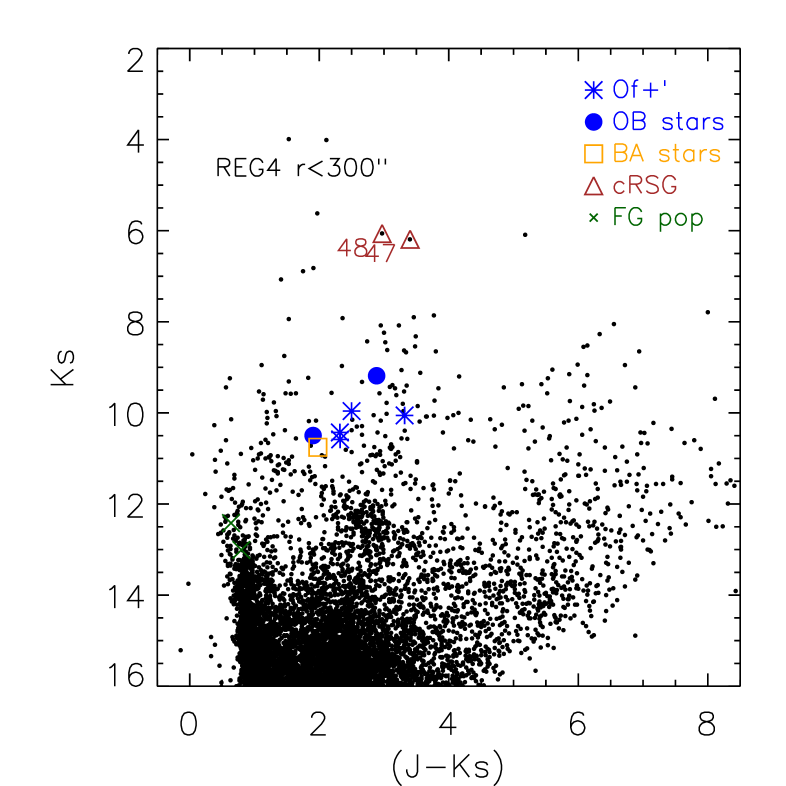
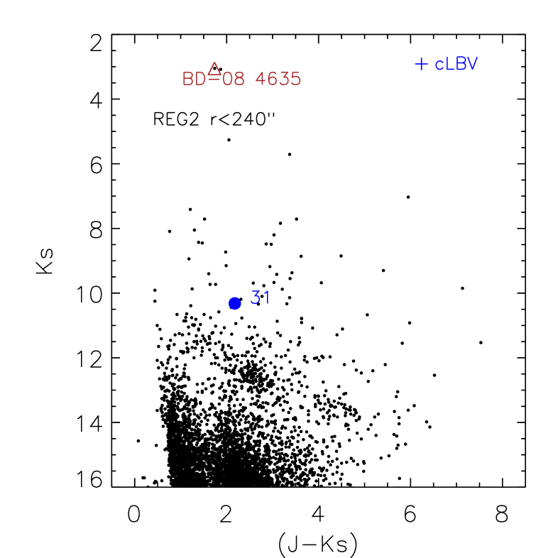
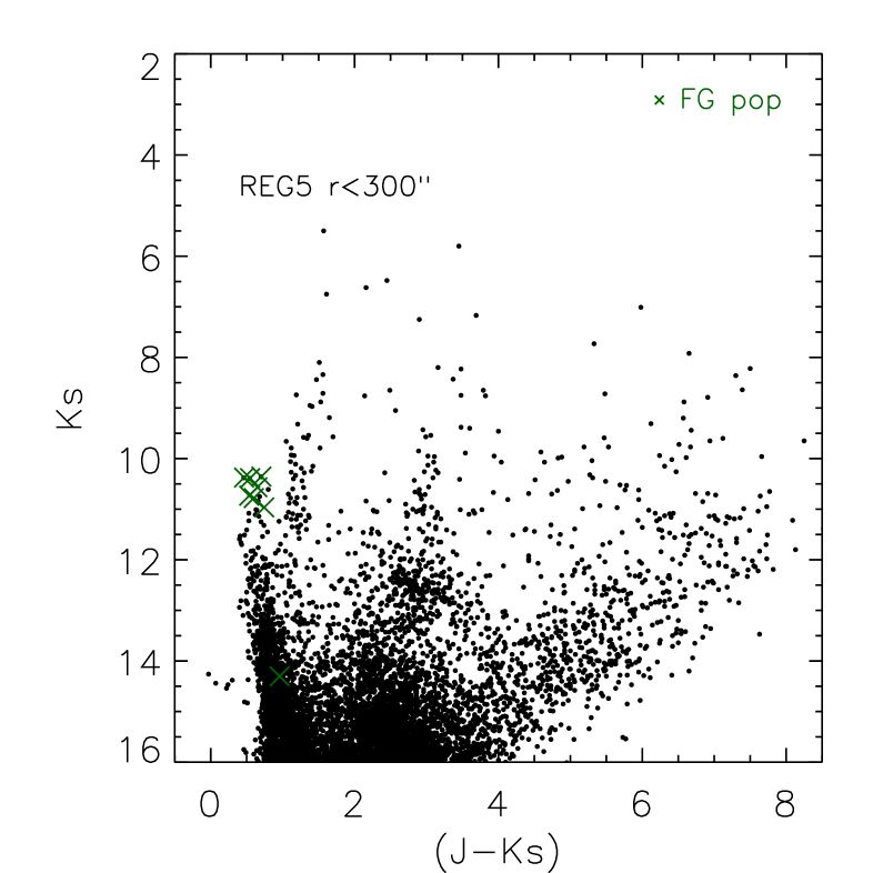
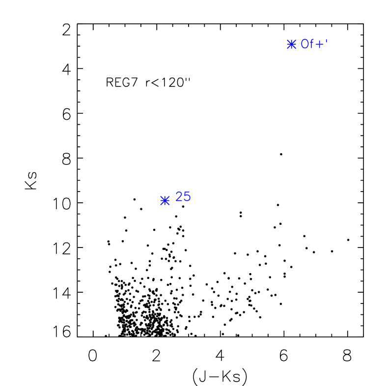
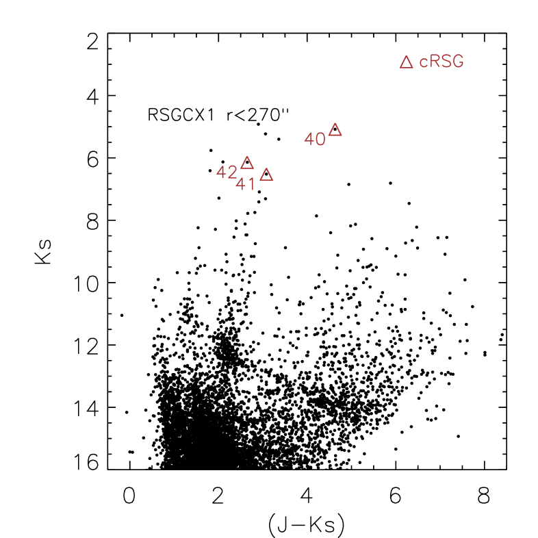
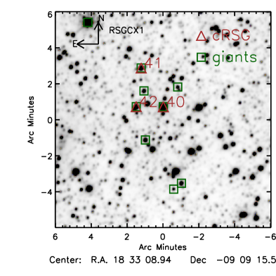
Figure 10: UKIDSS-2MASS K_s versus $J-$K_s diagrams of regions REG2 (top-right), REG4 (top-left), REG5 (middle-left), REG7 (middle-right), RSGCX1 (bottom-left) from Table 1. 2MASS data are used for K_s brighter than 10.5 mag. Spectroscopically observed stars are labeled as summarized in the legend. Of${}_{K}^{+}$ stars are marked with asterisks, late-O and early-B types with circles, late-B and early-A stars with squares. Possible foreground early-types ( A${}_{\it K_{\rm s}}$$<0.8$ mag) are marked with crosses. Triangles indicate RSGs/cRSGs. The bottom-right panel shows a map (WISE 3.4 $\mu$m) of RSGCX1, where squares indicate the observed giants, and triangles the cRSGs.

3.8 REG2 and the new candidate LBV

Region REG2 contains an Hii region (Figs.  1, 8), as inferred from the mid-infrared emission and coincident radio continuum emission. Star #31 was detected on the Western edge of this Hii region. The CMD of REG2 presents structures similar to those in REG4 (see 3.7). The color and magnitude of star #31 overlap those of the massive early-types in REG4, with A${}_{\it K_{\rm s}}$= 1.27 mag and K_s=10.32 mag.

The cLBV #22 does not appear to be part of this Hii region, it lies about $5\hbox to0.0pt{.\hss}^{\prime}5$ away from star #31, and is not part of any visible cluster of stars. Star #22 has A${}_{\it K_{\rm s}}$=1.13 mag and K_s=7.63 mag (see Tables 2 and 9). We assumed a spectral range from B3I to B8I, which corresponds to an average effective temperature of $13200\pm 2300$ K. We used an average BC${}_{\it K_{\mathrm{s}}}$ of $-$1.09 mag, and a distance of 4.6 kpc; we derived M_bol$=-7.90$ mag, $M_{\it V}=M_{\it K}+V-K=-6.93$ mag, and L $=1.1\times 10^{5}$ L_⊙; intrinsic $V-K$ color is from Koornneef (1983) and Martins & Plez (2006). The star would be the faintest known cLBV (e.g. Clark et al. 2009; Messineo et al. 2012), but within error consistent with the minimum predicted luminosity of L $=1.6\times 10^{5}$ (Groh et al. 2013). By assuming a higher temperature (24500 K, similar to that of the peculiar WRA751 Garcia-Lario et al. 1998), we would derive an average BC${}_{\it K_{\mathrm{s}}}$ of $-2.97$ mag, M_bol$=-9.84\pm 0.64$ mag, L $=6.8\times 10^{5}$ L_⊙.

3.9 REG7, REG5, and RSGCX1

Region REG7 coincides with nebular emission (Figs.  1, 8), without a clear stellar concentration. It also coincides with the candidate cluster [BDS2003]117 (Bica et al. 2003). We observed star #25, which lies at the center of the nebula, and identified it as an O4If_K+ star with A${}_{\it K_{\rm s}}$= $1.34$ mag, and M_bol= $-9.14$ mag (for 4.6 kpc).

In region REG5, we detected early-type stars (#7, #12, #13, #19, #26, #28, and #32 ) from a blue sequence, with an average A${}_{\it K_{\rm s}}$= $0.35\pm 0.06$ mag, as shown in Fig. 10. Their K_s range from 10.36 to 10.96 mag. They are foreground to the stellar population of the GMC (for example, the GLIMPSE9 cluster has an A${}_{\it K_{\rm s}}$ of $1.6\pm 0.2$ mag).

Star #40 (M0I) has a broad EW(CO), and $Q1$=0.22 mag, which is a typical value for red supergiants (Clark et al. 2009; Messineo et al. 2012). It is located, along with stars #41 and #42, in direction of the center of SNR $22.7-0.2$, in region RSGCX1 (see Figs. 8 and 10). The three stars (#40,#41, and #42) have A${}_{\it K_{\rm s}}$ of 1.95, 1.27, and 1.03 mag, which imply distances larger than 4 kpc (Clark et al. 2009; Drimmel et al. 2003). By assuming that they are at the distance of 4.6 kpc, we derived M_bol$=-7.49$, $-5.51$, and $-5.65$ mag, respectively, and their likely association with the SNR. The presence of 3 cRSGs implies also the presence of a candidate massive cluster of stars ($>10000$ M_⊙, Clark et al. 2009).

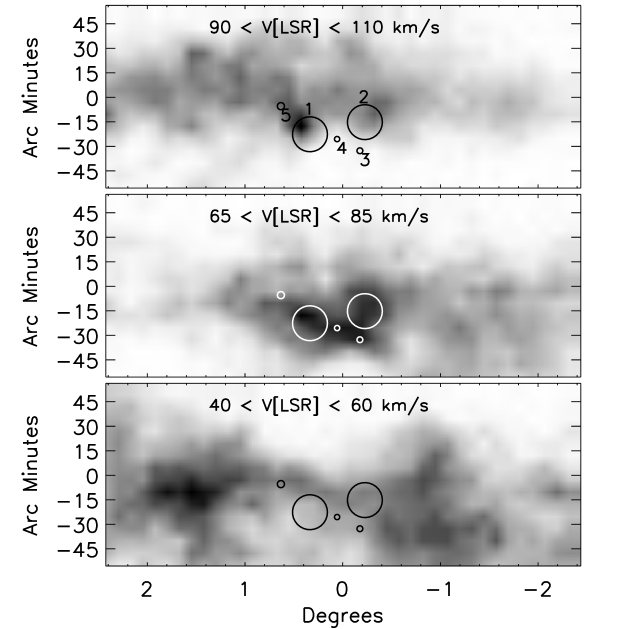
Figure 11: ¹²CO integrated maps in direction of the giant molecular complex $G23.3-0.3$ (Dame et al. 2001), from 40 km s^-1 to 60 km s^-1 (bottom panel), from 65 km s^-1 to 85 km s^-1 (middle panel), and from 90 km s^-1 to 110 km s^-1 ( top panel). Labels refer to SNR1, 2, 3, 4, and 5 in Table 11. Center is at a longitude of $22\hbox to0.0pt{.\hss}^{\circ}92$ and a latitude of $+0\hbox to0.0pt{.\hss}^{\circ}07$.

3.10 High-energy sources in the GMC and progenitor masses

Four SNRs are projected over the wide giant molecular cloud G23.3$-$0.3 (Messineo et al. 2010). In Figure 11, the SNRs are superimposed on a ¹²CO map of the giant molecular complex, with data-cubes from Dame et al. (2001). Several peaks of CO emission are seen, for example at velocity (in the local standard of rest system) of V_LSR$\approx 55$ km s^-1, $77-82$ km s^-1, and $100$ km s^-1; there is a similar velocity structure in the CO emission detected towards GLIMPSE09/SNR2, REG7/SNR3, REG5/SNR4, and REG4/W41. The prominent emission has a maximum peak at V_LSR= 77–82 km s^-1 (middle panel of Fig. 11); this is the cloud GMC G23.3$-$0.3, which is described by Albert et al. (2006) with a mass of about $2\times 10^{6}$ M_⊙ , and an extent of two degrees of longitude from $l\approx 22$^∘ to $l\approx 24\hbox to0.0pt{.\hss}^{\circ}25$, with a peak at $l\approx 23\hbox to0.0pt{.\hss}^{\circ}3$ and $b\approx-0\hbox to0.0pt{.\hss}^{\circ}3$; a strong velocity component at V_LSR$\approx 100$ km s^-1  (upper panel of Fig. 11) appears only in the two higher latitude regions (SNR1/W41 border, as measured by Brunthaler et al. (2009), and SNR2/SNR22.7$-$0.2).

Two SNRs with apparent diameters of $\sim$30^′ are listed in the catalogue of Green (2009), G022.7$-$00.2 (SNR2) and G023.3$-$00.3 (W41); two other highly probable shell SNRs with an angular diameter of $4\hbox to0.0pt{.\hss}^{\prime}7$ and $4\hbox to0.0pt{.\hss}^{\prime}5$, G$22.7583-0.4917$ (SNR3) and G$22.9917-0.3583$ (SNR4), were identified by Helfand et al. (2006) with MAGPIS data; their negative spectral indexes are also confirmed by Messineo et al. (2010). There is an extraordinary symmetry in the CO gas distribution of the giant cloud and locations (and even sizes) of the SNRs, which suggests their physical association with the cloud. Leahy & Tian (2008) concluded that W41 is associated with the GMC G23.3$-$0.3. G$22.7583-0.4917$ (SNR3) and G$22.9917-0.3583$ (SNR4) can similarly be associated with the GMC (Messineo et al. 2010); the SNR G23.5667$-$0.0333/SNR5 and G22.7$-$0.2 are at a slightly higher latitude, where the 77 km s^-1 and the $\sim$100 km s^-1 clouds overlap; however, at the position of G22.7$-$0.2 the 77 km s^-1 cloud has the strongest CO intensity (Messineo et al. 2010). The SNR G23.5667$-$0.0333/SNR5 (Helfand et al. 2006; Messineo et al. 2010) is located at $l=23\hbox to0.0pt{.\hss}^{\circ}57$ and $b=-0\hbox to0.0pt{.\hss}^{\circ}03$, outside the bulk of infrared emission of the main complex.

A large number of X-ray and TeV emitters have been reported in the direction of the two largest SNRs (W41/SNR1 and G22.7$-$0.2/SNR2). A schematic of the giant molecular cloud with the location of the SNRs, high-energy emitters, and the newly discovered massive stars is shown in Fig. 12 (see also Table 11).

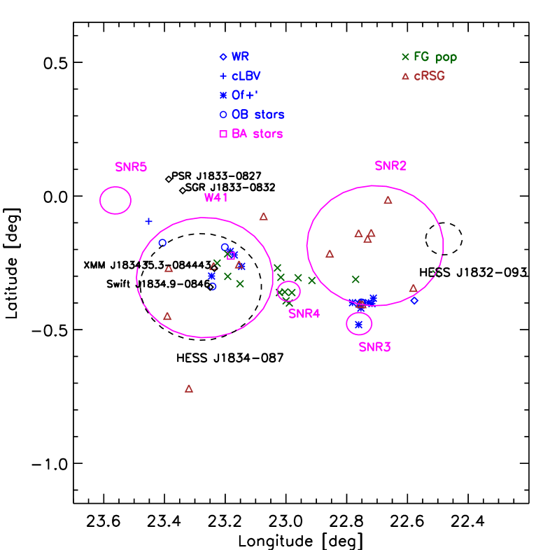
Figure 12: Locations and angular sizes of the supernova remnants (SNRs) are indicated with circles. Two dashed circles mark the positional uncertainties of HESS J1834$-$087 and HESS J1832$-$093. Dark diamonds indicates the location of PWN XMM-J183435.3$-$084443, Swift-J1834.9$-$0846, PSR J1833$-$0827, and SGR J1833$-$0832. Symbols used for stars are as in Fig. 8.

The TeV source HESS $J1834-087$ is located at the center of the shell-type remnant W41 (SNR1) (e.g. Aharonian et al. 2005; Tian et al. 2007; Leahy & Tian 2008). For the majority of extended TeV detections, young pulsars have been proposed as counterparts (young pulsar wind nebulae). Misanovic et al. (2011) identified the faint X-ray point-source XMM J183435.3$-$084443 (CXOU J183417.2$-$084901) (number 7 in Table 1 Mukherjee et al. 2009) as a pulsar wind nebula (PWN). Swift observations unveiled another possible TeV emitter, the magnetar Swift J1834.9$-$0846 (Gogus et al. 2011; Kargaltsev et al. 2012). So far, distances of 4-5 kpc have been assumed for both candidate TeV emitters by associating them with W41 (Leahy & Tian 2008).

HESS J1834$-$087, XMM J183435.3$-$084443, and Swift J1834.9$-$0846 fall in the center of the W41 shell, and in our region REG4 (see Fig. 8). In region REG4, we detected several rare O-type supergiants (from 28 to 45 M_⊙  at a spectro-photometric distance of 4.6 kpc) and two cRSGs. Swift J1834.9$-$0846 is one of the few Galactic magnetars associated with massive stars (.e.g. Figer et al. 2005; Bibby et al. 2008; Muno et al. 2006; Davies et al. 2009a; Mori et al. 2013).

SNR G22.7$-$0.2 has a size similar to that of W41 (40 pc at 4.6 kpc, Green 2009). The presence of a candidate cluster of RSGs (RSGCX1) with three cRSG stars toward the center of this SNR suggests that the progenitor of the supernova was from this population. HESS J1832$-$093 overlaps with SNR G22.7$-$0.2 (SNR2) (Laffon et al. 2011).

G22.7583-04917 (SNR3) has a diameter of about 5^′, or 6.7 pc at the distance of 4.6 kpc. The 90 cm shell-type emission is centered on the massive O4f_K+, star #25. This suggests that the SN progenitor had a mass similar to that of star #25 ($28-36$ M_⊙ at 4.6 kpc).

G22.9917$-$0.3583 (SNR4) has a size of about $4\hbox to0.0pt{.\hss}^{\prime}5$, or 6.0 pc at the distance of 4.6 kpc, and falls in region REG5 of Table 1. We detected only ”foreground stars”, which are unrelated to the GMC.

Table 11: List of associated high energy objects per supernovae remnants.

OBJECT	RA[J2000]	DEC[J2000]	diam	diam	Vel	Comment
	[hh mm ss]	[deg mm ss]	[′]	[pc]	[km s-1]
SNR1 / W41	18 34 46.42	$-$08 44 00	30	40.1	$77\pm 5$	3,6
HESS J1834-087	18 34 55.31	$-$08 44 17.64	12			1, 11, 13
PWN XMM J183435.3-084443	18 34 35.32	$-$08 44 43.80				12
PSR J1833-0827	18 33 40.35	$-$08 27 30.44				13
SGR J1833-0832	18 33 44.38	$-$08 31 07.71				4
Magnetar Swift J1834.9-0846	18 34 52.12	$-$08 45 55.97				5, 7
SNR2 / G22.7-0.2	18 33 17.86	$-$09 10 35	30	40.1	82.5	3, 6, 8
HESS J1832-093	18 32 46.85	$-$09 21 54.49	0.6			10
SNR3 -G22.7583-0.4917	18 34 26.70	$-$09 15 50	5.0	6.7	75.5	2, 3, 8, 9
SNR4 -G22.9917-0.3583	18 34 26.59	$-$09 00 09	4.5	6.0	70.9	3, 8, 9
SNR5 -G23.5667-0.0333	18 34 17.09	$-$08 20 21	6.1		91.3	3, 8, 9

• References. (1) Aharonian et al. (2005);  (2) Bronfman et al. (1996);  (3) Dame et al. (1986);  (4) Göğüş et al. (2010);  (5) Gogus et al. (2011);  (6) Green (2009);  (7) Kargaltsev et al. (2012);  (8) Kuchar & Clark (1997);  (9)Helfand et al. (2006);  (10)Laffon et al. (2011);  (11) Leahy & Tian (2008);  (12)Mukherjee et al. (2009);  (13) Tian et al. (2007).

4 Discussion and summary

4.1 Massive stars

Analysis of the spectroscopic data presented in this paper has revealed of a rich population of evolved massive stars associated with GMC G23.3$-$0.3, yielding 38 new early-type stars, 3 new RSGs, and 6 new cRSGs.

Complementary photometric data indicate a bi-modality in the distribution of A${}_{\it K_{\rm s}}$ of early-type stars. A component with A${}_{\it K_{\rm s}}$ from 0.9 to 2.0 mag contains a large variety of massive stars from O-types to late B-types, and a large fraction of those are associated with the GMC. The nine O- and B-type supergiants have average A${}_{\it K_{\rm s}}$=1.63 mag with $\sigma=0.18$ mag. Despite the uncertain absolute calibration of O-type stars, we obtained average spectro-photometric distance moduli from $13.18\pm 0.66$ mag (O9-9.5I) to $13.4\pm 0.4$ mag (Of_K+ stars). This range is consistent with that derived from B supergiants and with the distance to the GMC G23.3$-$0.3. We adopted a DM=$13.31\pm 0.17$ mag to characterize the luminosity and mass properties of obscured stars (A${}_{\it K_{\rm s}}$$>0.8$ mag), with the parallactic distance modulus of Brunthaler et al. (2009) in good agreement with the spectro-photometric distance.

Concerning the massive stellar cohort, a cLBV was detected in region REG2 and 10 massive Of_K+ stars in REG4 and in the vicinity of GLIMPSE9. The Of_K+ stars have K_so from 7.9 to 9.2 mag, and in Fig. 13 we plot their position on an HR diagram; comparison to theoretical predictions for rotating massive stars suggests masses from 25 to 45 M_⊙, and ages from 5 to 8 Myr (Ekström et al. 2012). This finding would suggest the likely presence of more evolved WRs in the complex; indeed, one WC8 is reported by Mauerhan et al. (2011).

RSGs have a large span of magnitudes even for an almost coeval population (for example, the RSGs in RSGC1, Figer et al. 2006), and are not suitable as distance indicators. By assuming a distance of 4.6 kpc, we found 3 new RSGs (#40, #43, and #47), ı.e. stars with luminosities larger than $>10^{4}$ M_⊙  and A${}_{\it K_{\rm s}}$  $>1.3$ mag. Their spectral types (from M0 to M2) closely align with the distribution of spectral types of Galactic RSGs, which peaks at M2-M3 (Davies et al. 2007; Elias et al. 1985). As shown in Figure 13, the new RSGs are much older than the detected O-stars; we estimated masses from 9 to 15 M_⊙ and ages from 20 to 30 M_⊙.

4.2 Distribution over the cloud

The location of the massive stars provides insights on the star formation history of GMC G23.3$-$0.3. The same mix of massive stars (RSGs, Of_K+ stars, and B stars) at similar A${}_{\it K_{\rm s}}$, spectral types, and magnitudes was detected in REG4 and GLIMPSE9Large. The two regions are separated by 27^′ (36 pc at 4.6 kpc). This provides evidence for repeated multi-seeded bursts of star formation across the complex, which appears to form a unique extended structure at a distance of about 4.6 kpc. Two main generations of massive stars were located; RSGs and cRSGs have ages of 20-30 Myr; massive Of_K+ stars trace star formation occurred 5-8 Myr ago.

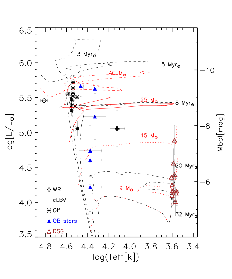
Figure 13: Luminosities of massive stars with A${}_{\it K_{\rm s}}$$>$0.8 mag are plotted versus their effective temperatures. Stellar tracks for stars of 9, 15, 25, and 40 M_⊙, based on the new rotating Geneva models with a solar metallicity, are shown with dotted and dashed lines; darker curves show the corresponding isochrones at 32, 20, 8, 5, and 3 Myr (Ekström et al. 2012). The positions of Of_K+ stars are marked by asterisks, the cLBV by a plus sign, the WR number 39 in Mauerhan et al. (2011) by a diamond symbol, other OB stars by filled triangles, and RSGs and cRSGc by empty triangles.

The luminosities of the 4 RSGs in GMC G23.3$-$0.3 (two new ones, plus the two RSGs in Messineo et al. 2010) are consistent with ages from 18 to 30 Myr. It is difficult to accurately infer the mass of the natal stellar aggregate of RSGs, because of their short lifetimes leading to a small population potentially affected by stochastic effects. Following the analysis by Clark et al. (2009), we might reasonably expect them to be associated with a population of stars of $>>10^{4}M_{\odot}$. Under the assumption of a Salpeter initial mass function (Salpeter 1955), we determine that additional stellar populations of total mass $\sim 2200$ and $\sim 1500$ M_⊙ were necessary to account for the presence of the six Of_K+ stars in region GLIMPSE9Large, and four in region REG4, respectively.

The G$23.3-0.3$ complex contains only one stellar cluster, GLIMPSE9, with a mass of $\sim 3000$ M_⊙ and an age of 15-27 Myr. The younger Of_K+ stars are not part of a stellar cluster and are distributed sparsely over two regions with radii of about 8.0 pc, with six surrounding the GLIMPSE9 cluster. A few examples of isolated massive star formation are reported in literature. For example, one O2If*/WN6 star with a mass of 40-80 M_⊙ (0.6 Myr old) and an O2If*/WN6 with mass $>100$ M_⊙ were detected in the Hii region surrounding the Galactic cluster NGC3603 (Roman-Lopes 2013b, a, 2012). Further observations will be required to understand the origin of this population.

We, therefore, infer a substantial difference in ages between the young massive stars (about 5 Myr) and older RSGs (18-30 Myr) in GMC G$23.3-0.3$. An age spread is common seen in giant molecular complexes, such as G305 (Clark & Porter 2004; Davies et al. 2012), W51 (Clark et al. 2009) and 30 Dor. The latter region is of particular interest with regard to GMC G$23.3-0.3$, with star formation apparently commencing $\sim$25Myr ago and continuing to the present day (Walborn & Blades 1997; Grebel & Chu 2000; Walborn et al. 2013).

Finally, the G$23.3-0.3$ complex is located at 23^∘, at a Galactocentric distance of about 4.6 kpc. The existence of a number of massive clusters/complexes rich in RSGs from $l\approx 23$^∘ to $l\approx 35$^∘  seems a peculiar feature of the Galactic barred potential (e.g. Nakashima & Deguchi 2006; Habing et al. 2006; Clark et al. 2009; Davies et al. 2009b).

4.3 Progenitor masses of SNRs

Adopting the initial mass function of Salpeter (1955) and employing the isochrones of Ekström et al. (2012), at an age of 5 Myr a representative stellar population will have lost $\sim 2$ ‰ of stars with masses $>1$ M_⊙ and 3.5% of stars with masses $>8$ M_⊙ as SNe; at 30 Myr these fractions increase to 3% and 45%, respectively. As such, we would expect multiple SNe to have occurred within G23.3$-$0.3; indeed, four of the 274 known SNR (Green 2014) are found to reside in it. We detected massive evolved stars towards the centers of SNR W41, G22.7$-$0.2(SNR2), and G22.7583$-$0.4917 (SNR3). Massive O stars (5-8 Myr) and RSGs (20-30 Myr) were detected in the center of W41; several candidate RSG stars were found in the center of G22.7$-$0.3/SNR2; a O4 supergiant in isolation was found at the center of G22.7583$-$0.4917 (SNR3).

Appendix A $Q1$ parameter

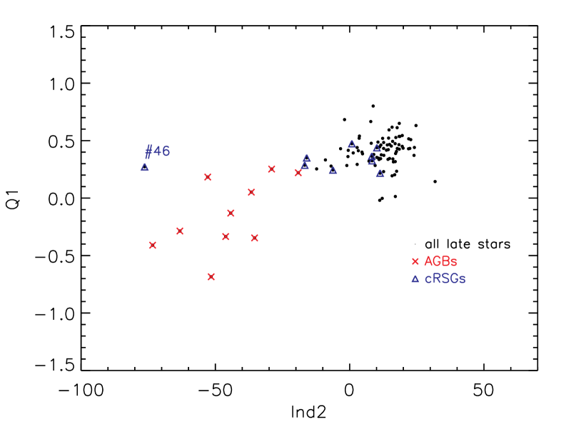
Figure 14: $Q1$ values of late-type stars (dots) versus the H₂O water index. We marked the AGB stars with crosses, and the cRSGs with triangles.

$Q1$ is defined as a combination of $J,H$ and K_s magnitudes, and it is proportional to the distance of a point-source from the interstellar reddening vector passing trough the origin in the $J-H$ versus $H-$K_s plane (Messineo et al. 2012); positive values are for point-sources to the left of the reddening vector, negative to the right. The reddening vector is defined with a power law and an index of $-1.9$ (Messineo et al. 2005).

$Q1$ values are plotted against H₂O water indexes in Fig.  14. Gaseous water absorption in the envelopes of late-type stars (for example Mira-type AGB stars) causes a dimming of the $H$ magnitude, and results in a weaker $Q1$ value. The average and standard deviation of the $Q1$ values of RSGs and cRSGs (L $>1\times 10^{4}$ L_⊙ for a distance of 4.6 kpc) are 0.38 and 0.11 mag, respectively; those of AGBs are $-0.15$ and 0.31 mag.

Appendix B Giant stars and selection of AGB stars

In $K-$band spectra of AGBs, absorption by water is visible as a change in shape of the stellar continuum short-ward of 2.1 $\mu$m  (Blum et al. 2003; Alvarez et al. 2000; Rayner et al. 2009). Some examples of $K$-band spectra of AGBs and RSGs are shown in Fig. 15.

We linearly interpolated the de-reddened spectra from 2.15 $\mu$m to 2.29 $\mu$m, extrapolated this fit to 2.0 $\mu$m, and calculated the difference of the linear fit and the observed spectrum from 2.0 $\mu$m to 2.1 $\mu$m; we defined the sum of this difference vector as the H₂O index. The distribution of the H₂O values resembles a gaussian with an additional tail of negative values. We classified as AGB stars those stars with a H₂O index deviating more than 6 $\sigma$ from the central mean. The same classification is obtained in the region 2.025-2.100 $\mu$m. A variation of 10% in the A${}_{\it K_{\rm s}}$ results in a typical variation of the H₂O index within 20%. This criterium reproduces the ”visual selection” of highly curved spectra. Stars #55, #56, #58, #60, #61, #62, #63, #65, #104, #134, #147, and #149 were classified as AGB stars, i.e. 12 out of 113 observed late-type stars (11%). AGB stars are listed in Tables 3 and 12.

Star #46 (#8 star in Messineo et al. 2010) is the brightest star of the GLIMPSE9 cluster in K_s-band. Despite its curved stellar continuum, it was classified as a likely RSG by comparison of its luminosity and extinction to those of other cluster members; its spectrum resembles My CEP (a rare M7I, Rayner et al. 2009).

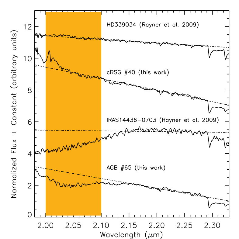
Figure 15: Normalized reddened spectra (arbitrarily shifted for clarity) of late-type stars. As an example, the spectrum of a new cRSG, #40, is compared to the IRTF spectrum of HD339034 (Rayner et al. 2009); the spectrum of the AGB #65 is compared to the IRTF spectrum of IRAS 14436-0703 (Rayner et al. 2009). The dotted-dashed lines are linear fits to the stellar continuum in the range 2.15-2.29 $\mu$m. The darker region is used for measuring an $H_{2}O$ index.

Appendix C Finding charts and giant stars

Finding charts for the detected stars are given in Figs. 16 and 17.

A list of detected red giant stars is provided in Table 12.

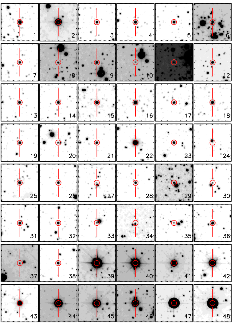
Figure 16: UKIDSS K-band images ( 30^′′$\times$ 30^′′) of the detected stars. Targets are indicated with 2 line-pointers. Identification numbers are from Tables 2,3, and 12. North is up and Est to the left.

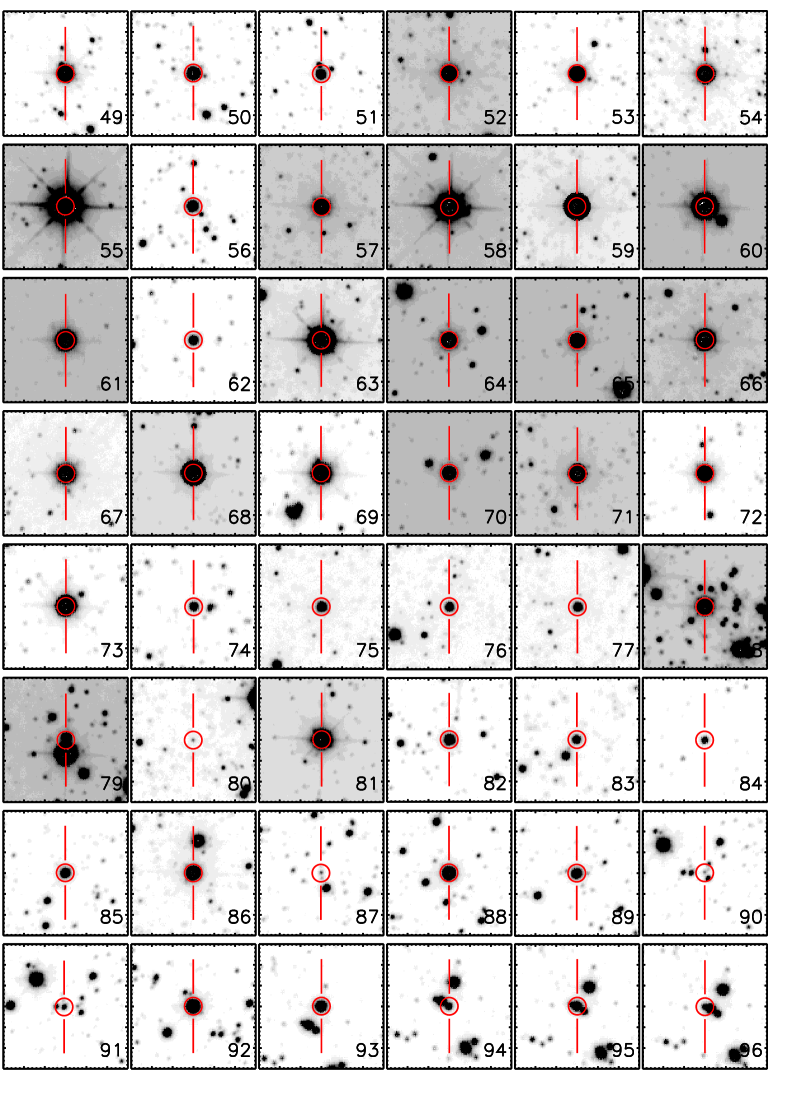
Figure 16: Figure 16 continued.

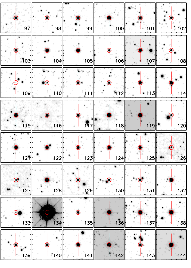
Figure 16: Figure 16 continued.

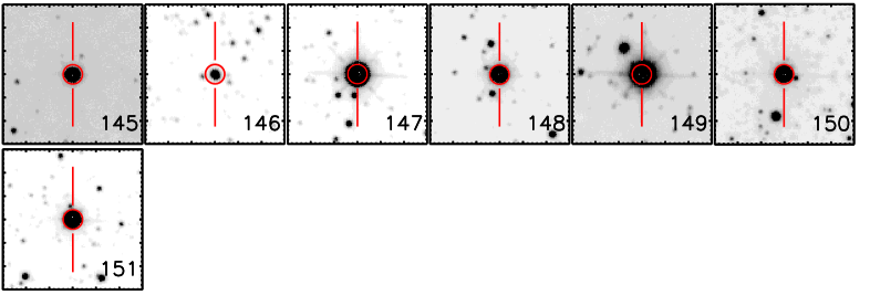
Figure 16: Figure 16 continued.

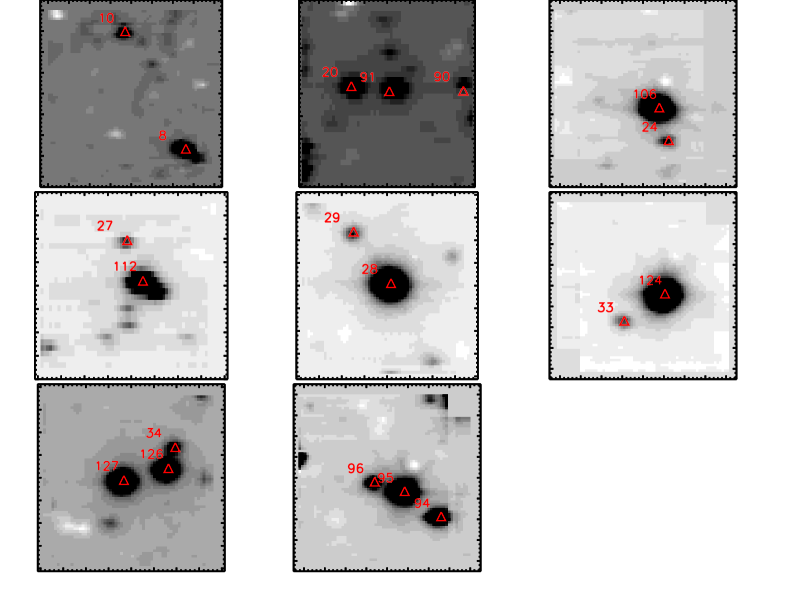
Figure 17: Average SINFONI cubes of faint early-type stars, which are difficult to identify in the UKIDSS images due to confusion. The SINFONI field of view is 8^′′$\times$ 8^′′, two cubes with a positional shift of $1\hbox to0.0pt{.\hss}^{\prime\prime}5$ were taken per observation. North is up and Est to the left of the image.

Table 12: List of observed giant stars ($L<4\times 10^{4}$L_⊙  for a distance of 4.6 kpc, or AGB stars).

ID	RA(J2000)	DEC(J2000)	Spectral Type					Comment
			Instr.	EW(CO)	Sp[giant]	Teff[giant]+	H2O
	[hh mm ss]	[deg mm ss]		[$AA$]		[K]	[%]
49	18 33 04.80	$-$9 12 47.7	SofI	25	M3	3605$\pm$ 120	8
50	18 33 05.64	$-$9 07 26.6	SofI	17	K3	3985$\pm$ 121	10
51	18 33 06.54	$-$9 13 07.4	SofI	28	M5	3450$\pm$ 203	16	BG
52	18 33 12.95	$-$9 10 23.3	SofI	23	M1	3745$\pm$ 130	1
53	18 33 13.27	$-$9 07 39.7	SofI	26	M4	3540$\pm$ 155	$-$3
54	18 33 13.82	$-$9 23 37.6	SofI	25	M3	3605$\pm$ 120	2
55	18 33 25.94	$-$9 03 51.2	SofI	27	$..$	$..$	$-$63	AGB
56	18 33 29.37	$-$8 51 22.9	SofI	35	$..$	$..$	$-$52	AGB
57	18 33 30.98	$-$8 50 27.0	SofI	24	M2	3660$\pm$ 140	$-$6
58	18 33 33.16	$-$8 48 15.8	SofI	28	$..$	$..$	$-$44	AGB IRAS 18307$-$0850
59	18 33 33.64	$-$9 13 51.5	SofI	26	M3	3605$\pm$ 120	13
60	18 33 38.69	$-$9 10 06.3	SofI	25	$..$	$..$	$-$46	AGB
61	18 33 40.24	$-$9 09 07.3	SofI	19	$..$	$..$	$-$51	AGB OH22.77-0.26a
62	18 33 40.97	$-$9 02 13.4	SofI	27	$..$	$..$	$-$25	AGB
63	18 33 41.07	$-$9 22 53.2	SofI	22	$..$	$..$	$-$73	AGB
64	18 33 44.64	$-$8 48 09.7	SofI	23	M1	3745$\pm$ 130	0
65	18 33 45.38	$-$8 47 57.7	SofI	21	$..$	$..$	$-$35	AGB
66	18 33 46.45	$-$9 21 36.1	SofI	25	M2	3660$\pm$ 140	10
67	18 33 46.75	$-$8 33 00.2	SofI	22	M0	3790$\pm$ 124	4
68	18 33 48.54	$-$9 12 36.2	SofI	24	M2	3660$\pm$ 140	8
69	18 33 48.82	$-$8 43 01.5	SofI	23	M1	3745$\pm$ 130	11
70	18 33 49.67	$-$8 33 05.9	SofI	25	M3	3605$\pm$ 120	2
71	18 33 49.92	$-$9 11 45.9	SofI	22	M1	3745$\pm$ 130	0
72	18 33 50.48	$-$8 42 42.1	SofI	23	M1	3745$\pm$ 130	10
73	18 33 53.33	$-$9 09 40.3	SofI	22	M1	3745$\pm$ 130	7
74	18 33 55.10	$-$9 08 12.3	SofI	22	M1	3745$\pm$ 130	10	BG
75	18 34 05.34	$-$8 56 56.5	SINFONI	42	M4	3540$\pm$ 155	18
76	18 34 05.47	$-$8 57 58.9	SINFONI	36	M1	3745$\pm$ 130	14
77	18 34 06.07	$-$8 57 10.7	SINFONI	37	M1	3745$\pm$ 130	24
78	18 34 09.28	$-$9 14 00.7	SINFONI	43	M4	3540$\pm$ 155	12	[MFD2010] 1b
79	18 34 10.37	$-$9 13 49.5	SINFONI	38	M2	3660$\pm$ 140	9	[MFD2010] 6b
80	18 34 11.46	$-$9 14 03.0	SINFONI	15	$<$ K0	$>$ 4185$\pm$ 204	$-$1
81	18 34 11.70	$-$8 57 09.3	SINFONI	48	M7	3223$\pm$ 226	$-$12
82	18 34 11.87	$-$8 57 29.4	SINFONI	39	M3	3605$\pm$ 120	11
83	18 34 12.10	$-$9 04 02.4	SINFONI	12	$<$ K0	$>$ 4185$\pm$ 204	15
84	18 34 14.70	$-$8 35 01.1	SINFONI	10	$<$ K0	$>$ 4185$\pm$ 204	$-$1	XMM$-$5 c
85	18 34 15.22	$-$8 47 41.3	SINFONI	38	M2	3660$\pm$ 140	17
86	18 34 15.79	$-$8 48 33.3	SINFONI	41	M4	3540$\pm$ 155	19
87	18 34 15.97	$-$8 45 41.6	SINFONI	34	M0	3790$\pm$ 124	3	BGd
88	18 34 16.03	$-$8 45 20.1	SINFONI	38	M2	3660$\pm$ 140	21
89	18 34 16.38	$-$8 46 19.0	SINFONI	35	M1	3745$\pm$ 130	23
90	18 34 18.52	$-$8 45 33.2	SINFONI	28	K3	3985$\pm$ 121	$..$
91	18 34 18.72	$-$8 45 33.0	SINFONI	25	K2	4049$\pm$ 131	7
92	18 34 19.19	$-$8 45 26.4	SINFONI	43	M5	3450$\pm$ 203	4
93	18 34 19.50	$-$9 04 35.5	SINFONI	27	K3	3985$\pm$ 121	16
94	18 34 19.58	$-$9 04 41.4	SINFONI	45	M5	3450$\pm$ 203	$..$
95	18 34 19.70	$-$9 04 40.1	SINFONI	26	K2	4049$\pm$ 131	17
96	18 34 19.79	$-$9 04 39.7	SINFONI	25	K2	4049$\pm$ 131	$..$
97	18 34 20.73	$-$8 48 49.0	SINFONI	37	M2	3660$\pm$ 140	3
98	18 34 21.42	$-$8 50 31.0	SINFONI	38	M2	3660$\pm$ 140	14
99	18 34 22.16	$-$9 14 16.0	SINFONI	38	M2	3660$\pm$ 140	14
100	18 34 23.13	$-$8 48 04.1	SINFONI	42	M4	3540$\pm$ 155	10

• Notes. The identification numbers are followed by celestial coordinates, instrument, EW(CO)s, spectral types, T_eff, H₂O indexes, and comments.  (⁺) Temperature erros account for accuracy in spectral types of $\pm 2$.  (^a) This Asymptotic giant branch stars (AGB) coincides with the maser OH22.77$-$0.26 (Blommaert et al. 1994). The stellar velocity (LSR) is 93.1 km s^-1.  (^b) Messineo et al. (2010).  (^c) XMM point source number 5 in Table 1 of Mukherjee et al. (2009).  (^d) BG= object in the background of the cloud.

Table 12: continuation of Table 12.

ID	RA(J2000)	DEC(J2000)	Spectral Type			Comment
			Instr.	Teff[giant]	Sp[giant]
	[hh mm ss]	[deg mm ss]			[K]
101	18 34 24.18	$-$9 14 34.0	SINFONI	34	M0	3790$\pm$ 124	18
102	18 34 24.26	$-$9 02 44.5	SINFONI	23	K1	4117$\pm$ 136	16
103	18 34 24.31	$-$8 47 38.9	SINFONI	34	M0	3790$\pm$ 124	17
104	18 34 24.39	$-$8 29 10.0	SofI	31	$..$	$..$	$-$32	AGB
105	18 34 25.86	$-$8 35 32.9	SINFONI	40	M3	3605$\pm$ 120	15
106	18 34 26.41	$-$9 00 47.6	SINFONI	20	$<$ K0	$>$ 4185$\pm$ 204	31
107	18 34 26.42	$-$8 47 18.4	SINFONI	36	M1	3745$\pm$ 130	22
108	18 34 27.65	$-$9 00 49.6	SINFONI	34	M0	3790$\pm$ 124	12
109	18 34 27.82	$-$9 00 52.8	SINFONI	33	M0	3790$\pm$ 124	$..$
110	18 34 29.48	$-$8 45 03.8	SINFONI	33	K5	3869$\pm$ 137	$..$
111	18 34 29.74	$-$8 45 03.7	SINFONI	40	M3	3605$\pm$ 120	12
112	18 34 30.10	$-$8 44 42.4	SINFONI	24	K1	4117$\pm$ 136	11
113	18 34 31.05	$-$8 51 41.2	SINFONI	39	M2	3660$\pm$ 140	21
114	18 34 31.70	$-$8 34 09.9	SINFONI	41	M3	3605$\pm$ 120	19
115	18 34 31.87	$-$8 47 14.8	SINFONI	37	M1	3745$\pm$ 130	14
116	18 34 32.31	$-$8 33 06.6	SINFONI	33	M0	3790$\pm$ 124	16
117	18 34 32.32	$-$8 34 03.0	SINFONI	38	M2	3660$\pm$ 140	17
118	18 34 32.48	$-$8 44 05.2	SINFONI	39	M2	3660$\pm$ 140	14
119	18 34 33.69	$-$8 32 39.8	SINFONI	39	M2	3660$\pm$ 140	19
120	18 34 33.73	$-$9 01 32.2	SINFONI	38	M2	3660$\pm$ 140	8
121	18 34 33.83	$-$9 17 56.9	SofI	22	M0	3790$\pm$ 124	17
122	18 34 33.93	$-$9 01 34.6	SINFONI	36	M1	3745$\pm$ 130	14
123	18 34 34.98	$-$8 33 08.0	SINFONI	34	M0	3790$\pm$ 124	16
124	18 34 35.61	$-$9 01 26.3	SINFONI	13	$<$ K0	$>$ 4185$\pm$ 204	12
125	18 34 36.73	$-$8 51 19.1	SINFONI	42	M4	3540$\pm$ 155	16
126	18 34 36.96	$-$8 47 55.6	SINFONI	28	K3	3985$\pm$ 121	$..$
127	18 34 37.10	$-$8 47 56.2	SINFONI	27	K3	3985$\pm$ 121	24
128	18 34 37.25	$-$9 17 44.5	SofI	20	K5	3869$\pm$ 137	8
129	18 34 37.67	$-$8 30 53.4	SINFONI	31	K5	3869$\pm$ 137	11
130	18 34 37.95	$-$8 50 48.7	SINFONI	48	M7	3223$\pm$ 226	2	BG
131	18 34 38.11	$-$8 50 50.5	SINFONI	31	K5	3869$\pm$ 137	17
132	18 34 38.72	$-$8 48 53.3	SINFONI	41	M3	3605$\pm$ 120	15
133	18 34 38.97	$-$8 48 52.5	SINFONI	47	M6	3336$\pm$ 226	$-$23	BG
134	18 34 39.18	$-$8 34 47.4	SofI	20	$..$	$..$	$-$36	AGB IRAS18318$-$0837
135	18 34 39.23	$-$8 49 08.8	SINFONI	32	K5	3869$\pm$ 137	15
136	18 34 39.55	$-$8 30 48.1	SINFONI	51	M7	3223$\pm$ 226	$-$9
137	18 34 39.58	$-$9 16 44.4	SofI	23	M1	3745$\pm$ 130	8
138	18 34 40.60	$-$9 14 45.9	SofI	22	M1	3745$\pm$ 130	14
139	18 34 41.35	$-$8 35 30.3	SINFONI	33	M0	3790$\pm$ 124	18
140	18 34 42.51	$-$8 35 34.7	SINFONI	16	$<$ K0	$>$ 4185$\pm$ 204	12
141	18 34 45.02	$-$8 47 23.5	SINFONI	33	M0	3790$\pm$ 124	18
142	18 34 47.45	$-$8 48 09.7	SINFONI	39	M2	3660$\pm$ 140	22
143	18 34 47.50	$-$8 47 33.9	SINFONI	38	M2	3660$\pm$ 140	17
144	18 34 48.09	$-$8 34 50.4	SINFONI	43	M4	3540$\pm$ 155	12
145	18 34 49.20	$-$8 34 22.4	SINFONI	38	M2	3660$\pm$ 140	18
146	18 35 14.66	$-$8 37 40.6	SINFONI	35	M0	3790$\pm$ 124	3	XMM$-$15 a
147	18 35 17.93	$-$8 29 54.1	SofI	26	$..$	$..$	$-$29	AGB
148	18 35 18.53	$-$8 29 10.7	SofI	23	M1	3745$\pm$ 130	3
149	18 35 21.28	$-$8 59 34.2	SofI	27	$..$	$..$	$-$19	AGB
150	18 35 27.04	$-$8 29 06.2	SofI	21	M0	3790$\pm$ 124	17
151	18 35 28.17	$-$8 28 34.7	SofI	19	K5	3869$\pm$ 137	11

• (^a) XMM point source number 15 in Table 1 of Mukherjee et al. (2009).

References

- Aharonian et al. (2005) Aharonian, F., Akhperjanian, A. G., Aye, K.-M., et al. 2005, Science, 307, 1938
- Albert et al. (2006) Albert, J., Aliu, E., Anderhub, H., et al. 2006, ApJ, 643, L53
- Alvarez et al. (2000) Alvarez, R., Lançon, A., Plez, B., & Wood, P. R. 2000, A&A, 353, 322
- Alves et al. (2007) Alves, J., Lombardi, M., & Lada, C. J. 2007, A&A, 462, L17
- Bibby et al. (2008) Bibby, J. L., Crowther, P. A., Furness, J. P., & Clark, J. S. 2008, MNRAS, 386, L23
- Bica et al. (2003) Bica, E., Dutra, C. M., Soares, J., & Barbuy, B. 2003, A&A, 404, 223
- Blommaert et al. (1994) Blommaert, J. A. D. L., van Langevelde, H. J., & Michiels, W. F. P. 1994, A&A, 287, 479
- Blum et al. (2000) Blum, R. D., Conti, P. S., & Damineli, A. 2000, AJ, 119, 1860
- Blum et al. (2003) Blum, R. D., Ramírez, S. V., Sellgren, K., & Olsen, K. 2003, ApJ, 597, 323
- Borissova et al. (2011) Borissova, J., Bonatto, C., Kurtev, R., et al. 2011, A&A, 532, A131
- Brand & Blitz (1993) Brand, J. & Blitz, L. 1993, A&A, 275, 67
- Brogan et al. (2006) Brogan, C. L., Gelfand, J. D., Gaensler, B. M., Kassim, N. E., & Lazio, T. J. W. 2006, ApJ, 639, L25
- Bronfman et al. (1996) Bronfman, L., Nyman, L.-A., & May, J. 1996, A&AS, 115, 81
- Brunthaler et al. (2009) Brunthaler, A., Reid, M. J., Menten, K. M., et al. 2009, ApJ, 693, 424
- Carpenter (2001) Carpenter, J. M. 2001, AJ, 121, 2851
- Carter (1990) Carter, B. S. 1990, MNRAS, 242, 1
- Churchwell et al. (2009) Churchwell, E., Babler, B. L., Meade, M. R., et al. 2009, PASP, 121, 213
- Clark et al. (2013) Clark, J. S., Bartlett, E. S., Coe, M. J., et al. 2013, A&A, 560, A10
- Clark et al. (2009) Clark, J. S., Davies, B., Najarro, F., et al. 2009, A&A, 504, 429
- Clark et al. (2003) Clark, J. S., Egan, M. P., Crowther, P. A., et al. 2003, A&A, 412, 185
- Clark & Porter (2004) Clark, J. S. & Porter, J. M. 2004, A&A, 427, 839
- Clark et al. (1999) Clark, J. S., Steele, I. A., Fender, R. P., & Coe, M. J. 1999, A&A, 348, 888
- Crowther et al. (2006) Crowther, P. A., Hadfield, L. J., Clark, J. S., Negueruela, I., & Vacca, W. D. 2006, MNRAS, 372, 1407
- Crowther et al. (1995) Crowther, P. A., Smith, L. J., Hillier, D. J., & Schmutz, W. 1995, A&A, 293, 427
- Cutri & et al. (2012) Cutri, R. M. & et al. 2012, VizieR Online Data Catalog, 2311, 0
- Cutri et al. (2003) Cutri, R. M., Skrutskie, M. F., van Dyk, S., et al. 2003, 2MASS All Sky Catalog of point sources.
- Dame et al. (1986) Dame, T. M., Elmegreen, B. G., Cohen, R. S., & Thaddeus, P. 1986, ApJ, 305, 892
- Dame et al. (2001) Dame, T. M., Hartmann, D., & Thaddeus, P. 2001, ApJ, 547, 792
- Davies et al. (2012) Davies, B., Clark, J. S., Trombley, C., et al. 2012, MNRAS, 419, 1871
- Davies et al. (2007) Davies, B., Figer, D. F., Kudritzki, R.-P., et al. 2007, ApJ, 671, 781
- Davies et al. (2009a) Davies, B., Figer, D. F., Kudritzki, R.-P., et al. 2009a, ApJ, 707, 844
- Davies et al. (2009b) Davies, B., Origlia, L., Kudritzki, R.-P., et al. 2009b, ApJ, 696, 2014
- de Wit et al. (2005) de Wit, W. J., Testi, L., Palla, F., & Zinnecker, H. 2005, A&A, 437, 247
- Drimmel et al. (2003) Drimmel, R., Cabrera-Lavers, A., & López-Corredoira, M. 2003, A&A, 409, 205
- Egan et al. (2002) Egan, M. P., Clark, J. S., Mizuno, D. R., et al. 2002, ApJ, 572, 288
- Egan et al. (2003) Egan, M. P., Price, S. D., Kraemer, K. E., et al. 2003, VizieR Online Data Catalog, 5114, 0
- Eisenhauer et al. (2003) Eisenhauer, F., Abuter, R., Bickert, K., et al. 2003, in Society of Photo-Optical Instrumentation Engineers (SPIE) Conference Series, Vol. 4841, Society of Photo-Optical Instrumentation Engineers (SPIE) Conference Series, ed. M. Iye & A. F. M. Moorwood, 1548–1561
- Ekström et al. (2012) Ekström, S., Georgy, C., Eggenberger, P., et al. 2012, A&A, 537, A146
- Elias et al. (1985) Elias, J. H., Frogel, J. A., & Humphreys, R. M. 1985, ApJS, 57, 91
- Epchtein et al. (1994) Epchtein, N., de Batz, B., Copet, E., et al. 1994, Ap&SS, 217, 3
- Fariña et al. (2009) Fariña, C., Bosch, G. L., Morrell, N. I., Barbá, R. H., & Walborn, N. R. 2009, AJ, 138, 510
- Figer et al. (2006) Figer, D. F., MacKenty, J. W., Robberto, M., et al. 2006, ApJ, 643, 1166
- Figer et al. (1995) Figer, D. F., McLean, I. S., & Morris, M. 1995, ApJ, 447, L29
- Figer et al. (1997) Figer, D. F., McLean, I. S., & Najarro, F. 1997, ApJ, 486, 420
- Figer et al. (2005) Figer, D. F., Najarro, F., Geballe, T. R., Blum, R. D., & Kudritzki, R. P. 2005, ApJ, 622, L49
- Figer et al. (2002) Figer, D. F., Najarro, F., Gilmore, D., et al. 2002, ApJ, 581, 258
- Garcia-Lario et al. (1998) Garcia-Lario, P., Riera, A., & Manchado, A. 1998, A&A, 334, 1007
- Gogus et al. (2011) Gogus, E., Kouveliotou, C., Kargaltsev, O., & Pavlov, G. 2011, The Astronomer’s Telegram, 3576, 1
- Göğüş et al. (2010) Göğüş, E., Cusumano, G., Levan, A. J., et al. 2010, ApJ, 718, 331
- Grebel & Chu (2000) Grebel, E. K. & Chu, Y.-H. 2000, AJ, 119, 787
- Green (2009) Green, D. A. 2009, Bulletin of the Astronomical Society of India, 37, 45
- Green (2014) Green, D. A. 2014, in IAU Symposium, Vol. 296, IAU Symposium, ed. A. Ray & R. A. McCray, 188–196
- Groh et al. (2013) Groh, J. H., Meynet, G., & Ekström, S. 2013, A&A, 550, L7
- Gvaramadze et al. (2010) Gvaramadze, V. V., Kniazev, A. Y., Fabrika, S., et al. 2010, MNRAS, 405, 520
- Habing et al. (2006) Habing, H. J., Sevenster, M. N., Messineo, M., van de Ven, G., & Kuijken, K. 2006, A&A, 458, 151
- Hanson et al. (1996) Hanson, M. M., Conti, P. S., & Rieke, M. J. 1996, ApJS, 107, 281
- Hanson et al. (2005) Hanson, M. M., Kudritzki, R.-P., Kenworthy, M. A., Puls, J., & Tokunaga, A. T. 2005, ApJS, 161, 154
- Helfand et al. (2006) Helfand, D. J., Becker, R. H., White, R. L., Fallon, A., & Tuttle, S. 2006, AJ, 131, 2525
- Humphreys (1978) Humphreys, R. M. 1978, ApJ, 219, 445
- Humphreys & McElroy (1984) Humphreys, R. M. & McElroy, D. B. 1984, ApJ, 284, 565
- Indebetouw et al. (2005) Indebetouw, R., Mathis, J. S., Babler, B. L., et al. 2005, ApJ, 619, 931
- Johnson (1966) Johnson, H. L. 1966, ARA&A, 4, 193
- Kargaltsev et al. (2012) Kargaltsev, O., Kouveliotou, C., Pavlov, G. G., et al. 2012, ApJ, 748, 26
- Kleinmann & Hall (1986) Kleinmann, S. G. & Hall, D. N. B. 1986, ApJS, 62, 501
- Koornneef (1983) Koornneef, J. 1983, A&A, 128, 84
- Krumholz & Bonnell (2007) Krumholz, M. R. & Bonnell, I. A. 2007, ArXiv 0712.0828
- Kuchar & Clark (1997) Kuchar, T. A. & Clark, F. O. 1997, ApJ, 488, 224
- Lada & Lada (2003) Lada, C. J. & Lada, E. A. 2003, ARA&A, 41, 57
- Laffon et al. (2011) Laffon, H., Khélifi, B., Brun, F., et al. 2011, ArXiv 1110.6890
- Leahy & Tian (2008) Leahy, D. A. & Tian, W. W. 2008, AJ, 135, 167
- Lejeune & Schaerer (2001) Lejeune, T. & Schaerer, D. 2001, A&A, 366, 538
- Levesque et al. (2005) Levesque, E. M., Massey, P., Olsen, K. A. G., et al. 2005, ApJ, 628, 973
- Lucas et al. (2008) Lucas, P. W., Hoare, M. G., Longmore, A., et al. 2008, MNRAS, 391, 136
- Maíz Apellániz et al. (2007) Maíz Apellániz, J., Walborn, N. R., Morrell, N. I., Niemela, V. S., & Nelan, E. P. 2007, ApJ, 660, 1480
- Martins et al. (2007) Martins, F., Genzel, R., Hillier, D. J., et al. 2007, A&A, 468, 233
- Martins et al. (2008) Martins, F., Hillier, D. J., Paumard, T., et al. 2008, A&A, 478, 219
- Martins & Plez (2006) Martins, F. & Plez, B. 2006, A&A, 457, 637
- Mauerhan et al. (2011) Mauerhan, J. C., Van Dyk, S. D., & Morris, P. W. 2011, AJ, 142, 40
- Mercer et al. (2005) Mercer, E. P., Clemens, D. P., Meade, M. R., et al. 2005, ApJ, 635, 560
- Messineo et al. (2011) Messineo, M., Davies, B., Figer, D. F., et al. 2011, ApJ, 733, 41
- Messineo et al. (2010) Messineo, M., Figer, D. F., Davies, B., et al. 2010, ApJ, 708, 1241
- Messineo et al. (2005) Messineo, M., Habing, H. J., Menten, K. M., et al. 2005, A&A, 435, 575
- Messineo et al. (2012) Messineo, M., Menten, K. M., Churchwell, E., & Habing, H. 2012, A&A, 537, A10
- Messineo et al. (2007) Messineo, M., Petr-Gotzens, M. G., Schuller, F., et al. 2007, A&A, 472, 471
- Misanovic et al. (2011) Misanovic, Z., Kargaltsev, O., & Pavlov, G. G. 2011, ApJ, 735, 33
- Modigliani et al. (2007) Modigliani, A., Hummel, W., Abuter, R., et al. 2007, ArXiv 0701297 / Proceedings ADA IV, 2006
- Mori et al. (2013) Mori, K., Gotthelf, E. V., Zhang, S., et al. 2013, ApJ, 770, L23
- Morris et al. (1996) Morris, P. W., Eenens, P. R. J., Hanson, M. M., Conti, P. S., & Blum, R. D. 1996, ApJ, 470, 597
- Mukherjee et al. (2009) Mukherjee, R., Gotthelf, E. V., & Halpern, J. P. 2009, ApJ, 691, 1707
- Muno et al. (2006) Muno, M. P., Clark, J. S., Crowther, P. A., et al. 2006, ApJ, 636, L41
- Nakashima & Deguchi (2006) Nakashima, J.-i. & Deguchi, S. 2006, ApJ, 647, L139
- Nishiyama et al. (2006) Nishiyama, S., Nagata, T., Kusakabe, N., et al. 2006, ApJ, 638, 839
- Oliva & Origlia (1992) Oliva, E. & Origlia, L. 1992, A&A, 254, 466
- Price et al. (2001) Price, S. D., Egan, M. P., Carey, S. J., Mizuno, D. R., & Kuchar, T. A. 2001, AJ, 121, 2819
- Rayner et al. (2009) Rayner, J. T., Cushing, M. C., & Vacca, W. D. 2009, ApJS, 185, 289
- Reid et al. (2009) Reid, M. J., Menten, K. M., Zheng, X. W., et al. 2009, ApJ, 700, 137
- Reunanen et al. (2007) Reunanen, J., Tacconi-Garman, L. E., & Ivanov, V. D. 2007, MNRAS, 382, 951
- Rieke & Lebofsky (1985) Rieke, G. H. & Lebofsky, M. J. 1985, ApJ, 288, 618
- Roman-Lopes (2012) Roman-Lopes, A. 2012, MNRAS, 427, L65
- Roman-Lopes (2013a) Roman-Lopes, A. 2013a, MNRAS, 433, 712
- Roman-Lopes (2013b) Roman-Lopes, A. 2013b, MNRAS, 435, L73
- Rousselot et al. (2000) Rousselot, P., Lidman, C., Cuby, J.-G., Moreels, G., & Monnet, G. 2000, A&A, 354, 1134
- Salpeter (1955) Salpeter, E. E. 1955, ApJ, 121, 161
- Schreiber et al. (2004) Schreiber, J., Thatte, N., Eisenhauer, F., et al. 2004, in Astronomical Society of the Pacific Conference Series, Vol. 314, Astronomical Data Analysis Software and Systems (ADASS) XIII, ed. F. Ochsenbein, M. G. Allen, & D. Egret, 380
- Shara et al. (2012) Shara, M. M., Faherty, J. K., Zurek, D., et al. 2012, AJ, 143, 149
- Skiff (2013) Skiff, B. A. 2013, VizieR Online Data Catalog, 1, 2023
- Skinner et al. (1998) Skinner, C. J., Bergeron, L. E., Schultz, A. B., et al. 1998, in Society of Photo-Optical Instrumentation Engineers (SPIE) Conference Series, Vol. 3354, Society of Photo-Optical Instrumentation Engineers (SPIE) Conference Series, ed. A. M. Fowler, 2–13
- Smith (2002) Smith, N. 2002, MNRAS, 336, L22
- Soto et al. (2013) Soto, M., Barbá, R., Gunthardt, G., et al. 2013, A&A, 552, A101
- Stead & Hoare (2009) Stead, J. J. & Hoare, M. G. 2009, MNRAS, 400, 731
- Storey & Hummer (1995) Storey, P. J. & Hummer, D. G. 1995, MNRAS, 272, 41
- Sylvester et al. (1998) Sylvester, R. J., Skinner, C. J., & Barlow, M. J. 1998, MNRAS, 301, 1083
- Thackeray (1974) Thackeray, A. D. 1974, MNRAS, 168, 221
- Tian et al. (2007) Tian, W. W., Li, Z., Leahy, D. A., & Wang, Q. D. 2007, ApJ, 657, L25
- van der Hucht (2001) van der Hucht, K. A. 2001, VizieR Online Data Catalog, 3215, 0
- Vollmann & Eversberg (2006) Vollmann, K. & Eversberg, T. 2006, Astronomische Nachrichten, 327, 862
- Walborn et al. (2013) Walborn, N. R., Barbá, R. H., & Sewiło, M. M. 2013, AJ, 145, 98
- Walborn & Blades (1997) Walborn, N. R. & Blades, J. C. 1997, ApJS, 112, 457
- Wegner (1994) Wegner, W. 1994, MNRAS, 270, 229
- White et al. (2005) White, R. L., Becker, R. H., & Helfand, D. J. 2005, AJ, 130, 586
- Whitney (1983) Whitney, C. A. 1983, A&AS, 51, 463
- Wright et al. (2014) Wright, N. J., Parker, R. J., Goodwin, S. P., & Drake, J. J. 2014, MNRAS, 438, 639
- Zacharias et al. (2004) Zacharias, N., Monet, D. G., Levine, S. E., et al. 2004, in Bulletin of the American Astronomical Society, Vol. 36, American Astronomical Society Meeting Abstracts, 1418