A cosmological exclusion plot:
Towards model-independent constraints on modified gravity
from current and future growth rate data
Abstract
Most cosmological constraints on modified gravity are obtained assuming that the cosmic evolution was standard CDM in the past and that the present matter density and power spectrum normalization are the same as in a CDM model. Here we examine how the constraints change when these assumptions are lifted. We focus in particular on the parameter (also called ) that quantifies the deviation from the Poisson equation. This parameter can be estimated by comparing with the model-independent growth rate quantity obtained through redshift distortions. We reduce the model dependency in evaluating by marginalizing over and over the initial conditions, and by absorbing the degenerate parameter into . We use all currently available values of . We find that the combination , assumed constant in the observed redshift range, can be constrained only very weakly by current data, at 68% c.l. We also forecast the precision of a future estimation of in a Euclid-like redshift survey. We find that the future constraints will reduce substantially the uncertainty, , at 68% c.l., but the relative error on around the fiducial remains quite high, of the order of 30%. The main reason for these weak constraints is that is strongly degenerate with the initial conditions, so that large or small values of are compensated by choosing non-standard initial values of the derivative of the matter density contrast.
Finally, we produce a forecast of a cosmological exclusion plot on the Yukawa strength and range parameters, which complements similar plots on laboratory scales but explores scales and epochs reachable only with large-scale galaxy surveys. We find that future data can constrain the Yukawa strength to within 3% of the Newtonian one if the range is around a few Megaparsecs. In the particular case of models, we find that the Yukawa range will be constrained to be larger than Mpc or smaller than 2 Mpc (95% c.l.), regardless of the specific model.
I Introduction
Testing possible modifications of gravity at very large scales is currently one of the most interesting research activity in cosmology. Modifications of standard gravity are often modeled by introducing one or more additional mediating fields in the gravitational Lagrangian. One of the most well studied example is the so-called Horndeski theory, which adds to the Einstein-Hilbert Lagrangian a single scalar field that obey the most general second order equation of motion Horndeski (1974).
As shown in several papers (e.g. Amendola et al. (2008); De Felice et al. (2011); Silvestri et al. (2013); Zuntz et al. (2012)), a generic modification of gravity introduces at linear perturbation level two new functions that depend only on background time-dependent quantities and, in Fourier space, on the wavenumber . One function, that we denote here with (sometimes also called ), modifies the standard Poisson equation, while the second one, , the anisotropic stress or tilt, provides the relation between the two gravity potentials . In standard gravity, one has .
In the so-called quasi-static regime (i.e. for linear scales that are below the sound horizon) of the Horndeski models, and also in some cases Könnig et al. (2014) of bimetric models Hassan and Rosen (2012), the two functions take a particularly simple form and can be directly constrained through observations De Felice and Tsujikawa (2012); Amendola et al. (2013). In particular, one can use observations of weak lensing, redshift distortions and galaxy clustering to constrain or detect modifications of gravity at cosmological scales Amendola et al. (2014a).
One problem of these techniques is that often one makes explicitly or implicitly several assumptions that might not be warranted by current data. For instance, one often assumes that the behavior of the cosmological model before dark energy domination, i.e. essentially at any time except very recently, is the standard radiation and matter dominated universe. While we have at least some proof that the radiation epoch had to be close to standard, otherwise one would see deviations from the standard big bang nucleosynthesis and on the microwave background sky, we have much less robust data concerning the matter dominated era, in particular between decoupling and now. For instance, models in which the dark energy was a substantial fraction of the cosmic energy at high redshift Doran and Robbers (2006); Pettorino et al. (2013) cannot yet be excluded.
We identify in particular three assumptions that are very commonly made (at least one of them is included in, for instance, Gong (2008); Narikawa and Yamamoto (2010); Hirano et al. (2012); Shi et al. (2012); Macaulay et al. (2013); Samushia et al. (2013); Arkhipova et al. (2014); Steigerwald et al. (2014)) and which are certainly acceptable in some cases but that, in reality, are not necessariy warranted in more general gravity theories. First, we do not know what is the present value of the matter density fraction . If we take it from distance measurements (supernovae, baryon acoustic oscillation) then one should be aware that the observed quantity is the expansion rate and not the equation of state or . In fact, the EOS depends on assuming a value of , and viceversa Kunz and Sapone (2007). Of course if is parametrized by a small number of parameters then one can get also from the distance data, but the estimation will depend on the chosen parametrization. Moreover, cannot be determined without ambiguity with other techniques, e.g. from weak lensing (e.g. More et al. (2014)) or -ray temperature in clusters (e.g. Rapetti et al. (2013)), since these estimates always assume standard Newtonian gravity.
Second, we do not know what is the present value of the power spectrum amplitude . In fact, any estimate of , through e.g. weak lensing (see e.g. More et al. (2014)), cosmic microwave background (e.g. Ade et al. (2013)), or cluster abundances (see e.g. Rapetti et al. (2013), Planck Collaboration et al. (2013)), depends again on assuming a particular (normally, Newtonian), theory of gravity.
Third, when we obtain the theoretical behavior of the linear perturbation, by integrating the matter conservation equations, we need to assume some initial condition for the matter density contrast and the peculiar velocity divergence (or equivalently on and , the prime being from now on the derivative with respect to the e-folding time ). Typically, this problem is bypassed assuming that the evolution in the past (say, for redshifts ) was identical to a matter dominated universe so that and (of course since we are in the linear regime one can always choose freely one of the two inital conditions, say ). However, if we do not know the cosmological model in the past, we cannot fix . For instance, in some coupled dark matter-dark energy model the perturbations grow faster than in CDM during the matter epoch due to the fact that the dark energy field is not negligible (e.g. Amendola and Tocchini-Valentini (2001)); in this case . Similarly, in a Brans-Dicke model with coupling one has Nariai (1969); although has to be very large to pass local gravity constraints, if a screening mechanism is present these bounds becomes very weak.
In this paper we wish to examine what constraints one can still get on modified gravity, in particular on , when all three assumptions, on and , are lifted by marginalizing over all the non-degenerate parameters. We will consider both current data and forecasted data from a future experiment that approximates the Euclid111http://www.euclid-ec.org survey Laureijs et al. (2011). We call this a model-independent approach, although of course we are still making several model-dependent assumptions, like for instance that we are really dealing with linear scales in the sub-horizon regime and that matter is conserved. We also assume for simplicity that matter is a pressureless fluid and that the background is well approximated by a CDM behavior during the redshift range that we consider, although both these assumptions can be easily generalized. One has also to bear in mind that it is possible to modify gravity leaving the function unaltered (but not , when properly defined in the Jordan frame, see discussion in Saltas et al. (2014)) so that even finding does not guarantee Einsteinian gravity.
We use the data obtained through the redshift distortion method Percival and White (2009) and collected in Macaulay et al. (2013); More et al. (2014). This method does not rely on assuming standard gravity, contrary to methods based, for instance, on extrapolation from CMB data, on weak lensing, cluster abundances, or galaxy power spectra.
The conclusion is that both present and future data have little chance to set stringent constraints on if one wants to be as much model-independent as possible. We find in particular a strong degeneracy between the initial conditions and that allows both relatively large and small values of . It is important to remark that we simplified out task by setting constant in time (the space dependence is either ignored as well or introduced according to the Horndeski model, see below). If we include an arbitrary time dependence, then the constraints would evaporate completely for current data, since we would have one datum at each redshift and one free parameter per redshift plus initial conditions and . For future data, where one can in principle obtain several data points at different ’s for each redshift, the constraints would not disappear but weaken a lot, and even more so if the initial conditions are taken to be -dependent. Clearly, obtaining any constraint at all would be totally impossible if the function, instead of being restricted to follow the Horndeski form, were a completely arbitrary function of time and space.
This leaves one only two escape routes to obtain stronger constraints on modified gravity through cosmological observations at linear scales. The first one is to forget model-independency and assume specific modified gravity models. Then one can estimate the model-specific and the initial conditions and confine within a much narrower region. The second one is to use a different parameter to test modified gravity. In Ref. Amendola et al. (2013a) it has been shown that the anisotropic parameter is a useful probe of gravity since it is independent of and it can be estimated from observations through an algebraic relation, i.e. without the need of choosing initial conditions. It is moreover more deeply connected to modifications of gravity (rather than just clustering of dark energy) than Saltas et al. (2014). Due to these properties, can be estimated by future clustering and lensing data (or even from B-modes of the cosmic microwave background data Amendola et al. (2014b); Raveri et al. (2014)) to a precision of just one percent if assumed constant Amendola et al. (2014a). This is to be contrasted to the 30% relative errors that can be obtained on the combination when model-independency is at least partially taken into account.
II The Horndeski parameters
We are interested in the evolution of linear perturbations in the quasi-static limit (i.e. for scales significantly inside the cosmological horizon, , and inside the Jeans lenght of the scalar, , such that the terms containing dominate over the time-derivative terms). One has then the following equation of linear perturbation growth
| (1) |
where and . The prime denotes the derivative respect to . The function , the effective gravitational constant for matter, is defined as
| (2) |
In this paper we always assume either that baryons do not feel modifed gravity or that the local gravity experiments occur in an environment where the extra force is not felt; in either case, they do not set any useful constraint on the cosmological expression for .
Now we assume that the background is described by the CDM model, so we have:
| (3) |
where we distinguish here between the parameter that enters the background rate and the parameter that expresses the amount of clustered matter in Eq. (1). In a modified gravity theory, the two quantities are independent and should be clearly distinguished. A perfect knowledge of the expansion rate, e.g. through supernovae Ia, will determine and, if the particular form (3) is assumed, but says nothing about the clustered fraction of matter . For instance, if dark energy mediates an extra force, matter will not dilute as and the value of that one would obtain from (3) would be unrelated to the real matter content.
The Horndeski Lagrangian is the most general Lagrangian for a single scalar field which gives second-order equations of motion for both the scalar field and the metric on an arbitrary background. In the quasi-static limit of the Horndeski Lagrangian one obtains:
| (4) |
where are time dependent functions that can be explicitly obtained when the full Horndeski Lagrangian is given Amendola et al. (2013). The scale is an arbitrary pivot scale that we choose to be /Mpc.
Eq. (1) can be written as
| (5) |
This shows immediately that is fully degenerate with . In the following therefore we will only be able to constrain the quantity
| (6) |
Since our reference model is CDM with , the standard value of is 0.3. Similarly, when we take the specific Horndeski form (4), we will constrain the combination .
Now, the rate itself can be estimated with distance indicators only up to some uncertainty. In the following however we will simplify our task by assuming that the error on is actually already now negligible with respect to the errors on the other observational data. For current data this is not completely true so our estimate of the uncertainty on is actually a lower limit. As the main effect of a change in is through the left-hand-side factor in Eq. (5), one can estimate the additional error on induced by an error in to be , to be added in quadrature. Current supernovae can determine around with a relative error of 5-10%, so we can estimate an additional error on around 10-20%. Since the uncertainty we find is quite larger than this, we neglect the additional source of error from . For the future data, one can indeed assume that will be pretty fairly well determined up to better than a percent accuracy with future surveys and our lower limit will be closer to reality.
For the initial conditions on , we fix the irrelevant value with i.e. , while for the initial growth rate parameter we either fix it to unity (standard CDM) or adopt a uniform prior large enough to cover all the region in which the likelihood is significantly different from zero.
Two caveats are in order. First, the entire analysis of this paper deals with linear scales. However, the data points we employ are obtained averaging over various scales that include probably also some weakly non-linear region of the power spectrum. For instance, the effective wavenumber in the analysis of Ref. Beutler et al. (2013) is given as Mpc, which at the average redshift of 0.57 is marginally affected by non linearity. In Ref. Samushia et al. (2013) the analysis of the same data including only large linear scales leads to an estimate of which is consistent with, and only mildly more uncertain than, the one obtained including smaller scales, indicating that the non linear effects are still subdominant. In any case, properly dealing with non linearity would require a reanalysis of the raw clustering data and an estimate of the non-linear corrections to for non-standard model. Secondly, the data points have been obtained by assuming a particular background expansion in order to convert from redshift to distances. Here we assume a fiducial CDM background with which does not coincide exactly with the one employed in some of the real data analysis. The corrections induced by both the non-linear effects and the fiducial background mismatch are expected to be quite smaller than the rather large error that we obtain on our modified gravity parameters.
III Marginalization over
We build a data posterior by using two datasets, the current dataset and the forecast dataset. The current dataset includes all the independent published estimates of obtained with the redshift distortion method. It includes the data from 2dFGS, 6dFGS, LRG, BOSS, CMASS, WiggleZ and VIPERS, and spans the redshift interval from to , see Table 1 (see also Macaulay et al. (2013); More et al. (2014)). In some case the correlation coefficient between two samples has been estimated in Ref. Macaulay et al. (2013) and included in our analysis; when there are different published results from the same dataset in Table 1 we include only the more recent one. The forecast dataset approximates instead the accuracy of a future Euclid mission Laureijs et al. (2011); Amendola et al. (2013b) and it has been obtained in Ref. Amendola et al. (2014a) in the range from to . The growth rate data are given as a set of values at various redshifts, where
| (7) |
and where is the growth rate, is the growth factor normalized to unity today and is the present power spectrum normalization. We denote our theoretical estimates as . We build then the function
| (8) |
where is the covariant matrix of the data. The first step to implement our model-independent estimates is to marginalize over , since as already mentioned to estimate its value from current data one would need to know the gravitational theory. Marginalizing the likelihood over with uniform prior leads to a new posterior where
| (9) |
and where
| (10) | |||||
| (11) | |||||
| (12) |
This is the posterior distribution we will use in the following discussion.
| Survey | z | References | |
|---|---|---|---|
| 6dFGRS | 0.067 | 0.423 ± 0.055 | Beutler et al. (2012) Beutler et al. (2012) |
| LRG-200 | 0.25 | 0.3512 ± 0.0583 | Samushia et al (2012) Samushia et al. (2012) |
| 0.37 | 0.4602 ± 0.0378 | ||
| LRG-60 | 0.25* | 0.36650.0601 | Samushia et al (2012) Samushia et al. (2012) |
| 0.37* | 0.40310.0586 | ||
| BOSS | 1) 0.30 | 0.408 0.0552, | Tojeiro et al. (2012)Tojeiro et al. (2012) |
| 2) 0.60 | 0.433 0.0662 | ||
| WiggleZ | 1) 0.44 | 0.413 ± 0.080, | Blake (2011) Blake et al. (2012) |
| 2) 0.60 | 0.390 ± 0.063, | ||
| 3) 0.73 | 0.437 ± 0.072 | ||
| Vipers | 0.8 | 0.47 ± 0.08 | De la Torre et al (2013)de la Torre et al. (2013) |
| 2dFGRS | 0.13 | 0.46 ± 0.06 | Percival et al. (2004) Percival et al. (2004) |
| LRG | 0.35 | 0.445 ± 0.097 | Chuang and Wang (2013) Chuang and Wang (2013) |
| LOWZ | 0.32 | 0.3840.095 | Chuang at al (2013)Chuang et al. (2013) |
| CMASS | 0.57* | 0.348 ± 0.071 | |
| 0.57* | 0.423 ± 0.052 | Beutler et al (2014)Beutler et al. (2013) | |
| 0.57 | 0.4410.043 | Samushia et al (2014) Samushia et al. (2013) | |
| 0.57* | 0.450 ± 0.011 | Reid et al (2013)Reid et al. (2014) |
IV Current growth-rate data
Current growth data are not sufficient to provide -dependent information. In this case, therefore, we are forced to neglect the -dependence of . Moreover, again in view of the lack of sufficient statistics, we also fix the time dependence and assume that is just a constant over the redshift range of the observations. We have therefore just two parameters: and the initial condition . We will consider four cases, in increasing order of “model independence”. The first case is standard CDM gravity (), and and initial conditions both fixed to the fiducial model, Ade et al. (2013) and . Here the only free parameter is therefore (with an uniform prior in ). The second case is like the first one but with marginalization over . This case serves mainly to isolate the effect of the -marginalization and to see how much the best fit of changes if is estimated from the data themselves and not from Planck. From now on, we always fix the background evolution to a CDM with = 0.3, in agreement with observations and close to the Planck best fit Ade et al. (2013), and neglecting any uncertainty on it and we always include the marginalization over . In the third case, beside marginalizing over , we leave free to vary with an uniform prior for positive values. Finally, the fourth case is like the third one but now the initial growth rate is left free to vary.
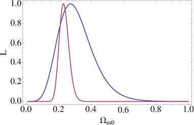
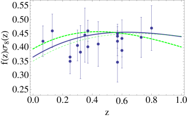
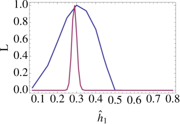
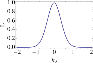
The results for the first and second cases are shown on the left panel of Fig. (1). At 68% c.l., the uncertainty on increases from 0.03 to roughly 0.10 when marginalizing over while for itself we find , smaller than but compatible with the Planck value. On the right panel, we plot the data points from the galaxy surveys with their respective error bars in comparison with the CDM model and with the best fits of all the cases.
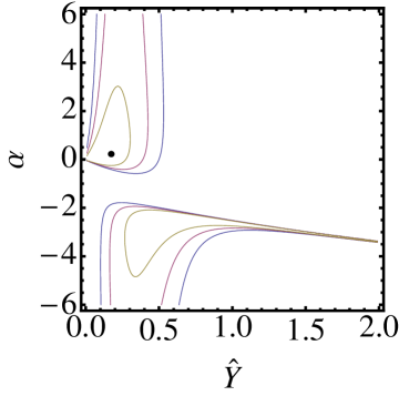
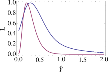
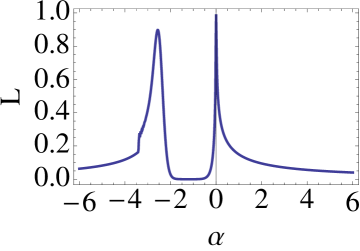
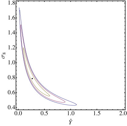
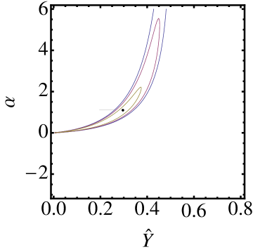
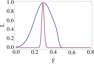
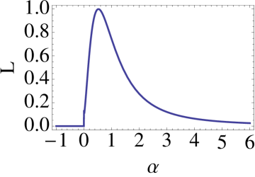
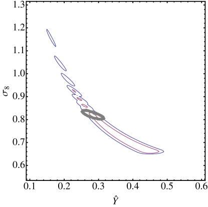
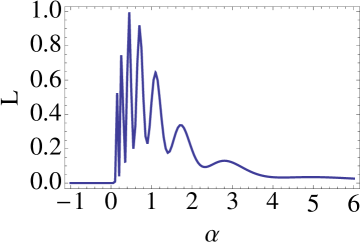
In the third case (uniform prior on , fixing ) we find a best fit with an error range at 68% confidence level, see Fig. (2) bottom left panel. The parameter is now , see Fig. (3). If now we vary with a uniform prior on (fourth case, Fig. 2) we obtain instead with a doubled error range at 68% c.l. . For we have now . Table (2) summarizes the results.
Interestingly, we detect a bimodality in the marginalized posterior for and a strong correlation with . As shown in Fig. (2) both very large and very small values of are acceptable if varies freely. In particular, a large can be compensated by a large negative , while small are compatible with large positive values. Large negative values of mean that overdensities can become underdensities at some point in time; although this might appear pathological at first sight, it does not contradict any observation at linear scales and should not be arbitrarily excluded. Within 3, a small is compatible with any value of since in this limit the perturbation equation becomes effectively first order in .
The conclusion of this section is that current data put hardly any constraint on . Any value from 0 to 1.35 is acceptable at 95% and much larger values of are also acceptable if the initial condition is chosen along the degeneracy line of Fig. (2).
This conclusion could have been reasonably expected due to the paucity of present data. In the next section we show however that the constraints improve a lot with the much better data of future surveys only if we keep fixed; in the more general case, the improvement remains modest. The reason is the same: trying to be as much model-independent as possible one has to set free to vary. The price to pay for this freedom are rather weak constraints.
| case | (95%) | (68%) | () | ( ) | |||
| (best fit) | (best fit) | ||||||
| CDM, , | I | 1 | - | - | 0.23 | [0.18, 0.29] | [0.20, 0.26] |
| CDM, , marg. on | II | 1 | - | - | 0.27 | [0.12, 0.54] | [0.18, 0.39] |
| case | () | () | |||||
| Uniform prior on | III | 1 | - | - | 0.20 | [0.040, 0.60] | [0.095, 0.36] |
| Uniform prior on | IV | -0.015 | -2.08 and | [-0.40, 1.32] and | 0.28 | [0, 1.35] | [0.048, 0.63] |
| -0.67 | [-4.05, -2.20] |
V Forecast data
A. binning
In this section we consider the forecast Euclid-like datasets, starting with the case of no scale information (-binning), which can be directly compared to the previous ones. The growth forecasts are obtained from Ref. Amendola et al. (2014a). We consider a Euclid-like 15,000 square degrees redshift survey from divided in equally spaced bins of width and, in order to prevent accidental degeneracy due to low statistic, a single larger redshift bin between , so in total we have six bins. In Table 3 we show the fiducial values and relative errors on .
| (68% c.l.) | ||
|---|---|---|
| 0.6 | 0.469 | 0.0092 |
| 0.8 | 0.457 | 0.0068 |
| 1.0 | 0.438 | 0.0056 |
| 1.2 | 0.417 | 0.0049 |
| 1.4 | 0.396 | 0.0047 |
| 1.8 | 0.354 | 0.0039 |
As before, we want to obtain an estimate on a constant marginalizing over and . Fig. (4), lower left panel, shows the 1-dimensional marginalized forecast posterior distribution of (third case) along with the fourth case, i.e. with marginalization over . As can be seen from Fig. (4), lower left panel, the 95% error on around the fiducial value 0.3 has a fivefold increase, from to roughly , when we marginalize over the initial conditions. The relative uncertainly on is around 30% at 68% c.l.. Contrary to what we found previously using current data, negative values of appear now strongly disfavoured.
The increase in errors on both and can be appreciated from Fig. (5). In the third case (i.e. no marginalization over ) future Euclid-like data can estimate and to within 0.01 for both parameters; when is marginalized over however the error increases to roughly , again for both parameters.
| case | Best fit | (95%) | (68%) | Best fit | () | () | |
|---|---|---|---|---|---|---|---|
| Uniform prior on | III | 1 | - | - | 0.29 | [0.26, 0.32] | [0.28, 0.30] |
| Uniform prior on | IV | 0.53 | [0, 4.0] | [0.12, 1.6] | 0.30 | [0.12, 0.43] | [0.21, 0.38] |
B. binning
We consider now the quasi-static Horndeski result, defined in Eq. (4), which contains the parameters , and and a dependence. Although in general these parameters depend on time, we assume here for simplicity that they time variation is negligible in the observed range. The aim of this section is to obtain error estimates on the Horndeski parameters, so we need to have a minimum of three -bins for every value of the redshift. Again following the method of Amendola et al. (2014a) we take the minimum binning value of as (the result is very weakly dependent on this value) and the values of the highest are chosen to be well below the scale of non-linearity at the redshift of the bin. In Table 5 we report the -bin boundaries.
In Table 6 we display the fiducial values and errors for at every redshift and every - bin. As in the previous case, also here the fiducial model is chosen to be CDM, so the fiducial values for the Horndeski parameters are and . Here we fix to its fiducial value (i.e. to zero) due to the degeneracy between and when the fiducial model is such that = as in CDM. In the next section we will consider the case in which the fiducial value of is different from the standard value.
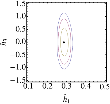
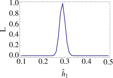
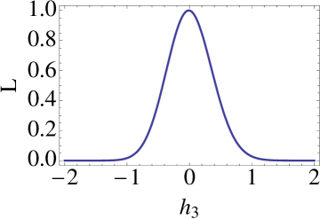
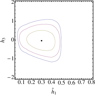
The model now contains three parameters: . Note that in principle one should take a different for every but for simplicity we assume that is -independent in our range. As in the previous cases, here we analyze first the case in which (this is our fifth case) and the case in which we will vary this parameter (sixth case). We numerically solve Eq. (1) inserting now the value of corresponding to the central -bin values for every redshift bin and then we construct the -marginalized three dimensional forecasted posterior by following the same procedure described in section III. The results are reported in Table 7 and in Figs. (6,7). The error on increase from roughly 0.02 to 0.10 when marginalizing over the initial condition. In contrast, the error on the scale remain practically unchanged, since we assume -independent initial conditions.
| 0.6 | 0.007-0.022 | 0.022-0.063 | 0.063-0.180 |
| 0.8 | 0.007-0.023 | 0.023-0.071 | 0.071-0.215 |
| 1.0 | 0.007-0.024 | 0.024-0.078 | 0.078-0.249 |
| 1.2 | 0.007-0.026 | 0.026-0.086 | 0.086-0.287 |
| 1.4 | 0.007-0.027 | 0.027-0.094 | 0.094-0.329 |
| 1.8 | 0.007-0.029 | 0.029-0.112 | 0.112-0.426 |
| 0.6 | 1 | 0.469 | 0.07 | 15 |
|---|---|---|---|---|
| 2 | 0.017 | 3.6 | ||
| 3 | 0.0097 | 2.1 | ||
| 0.8 | 1 | 0.457 | 0.05 | 11 |
| 2 | 0.012 | 2.6 | ||
| 3 | 0.0074 | 1.6 | ||
| 1.0 | 1 | 0.438 | 0.039 | 8.9 |
| 2 | 0.0089 | 2 | ||
| 3 | 0.0062 | 1.4 | ||
| 1.2 | 1 | 0.417 | 0.032 | 7.7 |
| 2 | 0.0072 | 1.7 | ||
| 3 | 0.0055 | 1.3 | ||
| 1.4 | 1 | 0.396 | 0.028 | 7 |
| 2 | 0.0065 | 1.6 | ||
| 3 | 0.0057 | 1.4 | ||
| 1.8 | 1 | 0.354 | 0.015 | 4.3 |
| 2 | 0.0047 | 1.3 | ||
| 3 | 0.0061 | 1.7 |
| case | (95%) | (68%) | (95%) | (68%) | (95%) | (68%) | ||||
|---|---|---|---|---|---|---|---|---|---|---|
| (best fit) | (best fit) | (best fit) | ||||||||
| Horndeski | V | 1 | - | - | 0.3 | [0.26, 0.32] | [0.27, 0.32] | 0 | [-0.70, 0.72] | [-0.37, 0.35] |
| Horndeski | VI | 0.85 | [0.10, 2.2] | [0.22, 1.9] | 0.3 | [0.097, 0.44] | [0.17, 0.40] | 0 | [-0.72, 0.73] | [-0.36, 0.36] |
VI A cosmological exclusion plot
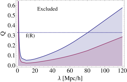
Here we wish to continue the analysis by obtaining an exclusion plot, i.e. the region of parameter space that a future Euclid-like redshift survey can achieve. This is obtained by repeating the procedure of the previous section obtaining the errors on for every possible (rather than fixing to the standard value). The region outside the errors is therefore the region that an Euclid-like experiment will be able to rule out.
The form of in Eq. (4) produced in a Horndeski model represents a Yukawa-like gravitational potential in real space. By Fourier anti-transforming Eq. (2) with a point source of mass one obtains in fact
| (13) |
where and (notice that here again is the observable, not alone). Here is the gravitational constant one would measure in laboratory where, as already mentioned, the effects of the modification of gravity are assumed to be screened 222Notice that although one could define a new gravitational “constant” in the potential, one should use a different definition, namely , in the force. This is why we prefer to use a different notation, i.e. ..
Thus, instead of , we can use the strength and range of the Yukawa term as modified-gravity parameters, marginalizing over and, as before, also over and . As previously, we assume to be constant in the observed range. These parameters are the cosmological analog of the parameters employed in laboratory experiments to test deviations from Newtonian gravity, see e.g. Kapner et al. (2007). Using the same specifications of the previous section, we show in Fig. (8) the region that a Euclid-like experiment is able to exclude. Clearly, for very small the strength is unconstrained; moreover, for very large interaction ranges (much larger than the observed scales), the strength becomes degenerate with and therefore again weakly constrained. In the intermediate region around 10 Mpc the strength can be confined to within 0.03 (0.06) at 68% (95%) c.l., i.e. 3% (6%) of the Newtonian gravitational strength. This limit is of course much weaker than local gravity bounds, which are below , but it applies to scales and epochs unreachable with other means. The results will not change much if we do not marginalize over initial conditions, just as it happened for in the previous section.
For comparison, the strength in the case of models is 1/3 (see e.g. De Felice and Tsujikawa (2010)), while the range is
| (14) |
where the subscripts denote the derivative with respecto to of the Lagrangian (in this notation includes the Einstein-Hilbert term). From Fig. (8) one can see that all the models with Mpc could be ruled out at 95% c.l. for . Conversely, assuming as needed by local gravity constraints and by a background close to CDM, a Euclid-like survey will be able to set a lower and an upper limit to :
| (15) | |||||
| (16) |
In keeping with our analysis, we are assuming here constant; in general however it will be a function of time so these limits should refer to the epoch of observation. In some popular models of one has at (see e.g. Jaime et al. (2012)), corresponding to Mpc, a value that could be marginally detected at 68% c.l. by our forecasts.
Notice however that in models the overall factor here denoted as corresponds to . The existence of a lower limit to is due to the marginalization over the unknown . In specific models of the present matter density can be estimated through background or large-scale structure measurements. In this case the lower limit would be removed and any larger than a few Megaparsec would be detected. The application of the results of this paper to specific models of modified gravity is left to future work.
VII Conclusions
In this paper we investigated the current and future bounds on the modified gravity parameter (or ) that quantifies the deviation from the standard Poisson equation. We have assumed to be constant in time and space when using current data or with a Horndeski behavior when forecasting future results. Contrary to other similar analyses, we tried to weaken the model-dependency by marginalizing over the present power spectrum normalization and over the initial growth rate for the matter density contrast equation, since they both are unknown unless one assumes a specific model, e.g. CDM. We also take into account the fact that is not a directly observable quantity and absorb it into the definition of .
We find, not unexpectedly, that the current growth rate data from redshift distortion are insufficient to constrain the product to better than an order of 100% error (see Table 2, fourth case), due to the degeneracy with and the initial condition. Using instead forecasts of a Euclid-like experiment, we find that the relative error on reduce to roughly 30% at 68% c.l. (see Table 4, fourth case). A similar error can be obtained on when using the Horndeski prescription (see Table 7, sixth case). The effect of the lack of knowledge of the initial conditions can be easily grasped by noting that the uncertainty on increases from when to when is marginalized over (Table 2), i.e. from a few percent to 30%. Same broadening of the uncertainty occurs for .
Finally, we obtain a forecast of a cosmological exclusion plot on the Yukawa strength and range parameters (Fig. 8). This complements, on cosmological scales, the laboratory exclusion plots on deviations from standard gravity. We find that with a Euclid-like experiment the strength can be confined to within 3%(6%) of the Newtonian gravity at 68%(95%) if the interaction range is around 10 Megaparsecs. For much larger and much smaller ranges the constraint gradually vanishes. Applying these results to models we forecast an upper limit to at of the order of , corresponding to a Yukawa range smaller than 2 Mpc roughly, and a lower limit of , corresponding to scales larger than Mpc (at 95% c.l.).
The main conclusion of this paper is that can be only weakly constrained by the next decade redshift surveys if one takes into account the degeneracy with and initial conditions. Even weaker constraints would have been obtained had we taken to be time dependent. Only by considering specific models can one hope to produce stringent constraints on modified gravity through its effect on linear matter perturbation growth. This seems to indicate that the other modified gravity linear perturbation parameter, the anisotropic stress , which requires a combination of weak lensing and clustering, is a more robust and powerful way to quantify the deviation from standard gravity.
Acknowledgements.
L.A. acknowledges support from DFG through the project TRR33 “The Dark Universe”. We thank Alejandro Guarnizo-Trilleras and Adrian Vollmer for help with the forecasts and Guillermo Ballesteros, Emilio Bellini, Valerio Marra and Valeria Pettorino for useful discussions. L.T. thanks the Institute of Theoretical Physics at the University of Heidelberg for the hospitality.References
- Horndeski (1974) Gregory Walter Horndeski, “Second-order scalar-tensor field equations in a four-dimensional space,” Int.J.Th.Phys. 10, 363–384 (1974).
- Amendola et al. (2008) L. Amendola, M. Kunz, and D. Sapone, “Measuring the dark side (with weak lensing),” JCAP 4, 013 (2008), arXiv:0704.2421 .
- De Felice et al. (2011) Antonio De Felice, Tsutomu Kobayashi, and Shinji Tsujikawa, “Effective gravitational couplings for cosmological perturbations in the most general scalar-tensor theories with second-order field equations,” Phys.Lett. B706, 123–133 (2011), arXiv:1108.4242 [gr-qc] .
- Silvestri et al. (2013) Alessandra Silvestri, Levon Pogosian, and Roman V. Buniy, “A practical approach to cosmological perturbations in modified gravity,” (2013), arXiv:1302.1193 [astro-ph.CO] .
- Zuntz et al. (2012) J. Zuntz, T. Baker, P. G. Ferreira, and C. Skordis, “Ambiguous tests of general relativity on cosmological scales,” J. Cosmology Astropart. Phys 6, 032 (2012), arXiv:1110.3830 [astro-ph.CO] .
- Könnig et al. (2014) Frank Könnig, Yashar Akrami, Luca Amendola, Mariele Motta, and Adam R. Solomon, “Stable and unstable cosmological models in bimetric massive gravity,” (2014), arXiv:1407.4331 [astro-ph.CO] .
- Hassan and Rosen (2012) S.F. Hassan and Rachel A. Rosen, “Resolving the Ghost Problem in non-Linear Massive Gravity,” Phys.Rev.Lett. 108, 041101 (2012), arXiv:1106.3344 [hep-th] .
- De Felice and Tsujikawa (2012) Antonio De Felice and Shinji Tsujikawa, “Conditions for the cosmological viability of the most general scalar-tensor theories and their applications to extended Galileon dark energy models,” JCAP 1202, 007 (2012), arXiv:1110.3878 [gr-qc] .
- Amendola et al. (2013) L. Amendola, M. Kunz, M. Motta, I. D. Saltas, and I. Sawicki, “Observables and unobservables in dark energy cosmologies,” Phys. Rev. D 87, 023501 (2013), arXiv:1210.0439 [astro-ph.CO] .
- Amendola et al. (2014a) Luca Amendola, Simone Fogli, Alejandro Guarnizo, Martin Kunz, and Adrian Vollmer, “Model-independent constraints on the cosmological anisotropic stress,” Phys.Rev. D89, 063538 (2014a), arXiv:1311.4765 [astro-ph.CO] .
- Doran and Robbers (2006) Michael Doran and Georg Robbers, “Early dark energy cosmologies,” JCAP 0606, 026 (2006), arXiv:astro-ph/0601544 .
- Pettorino et al. (2013) V. Pettorino, L. Amendola, and C. Wetterich, “How early is early dark energy?” arXiv:1301.5279 (2013), arXiv:1301.5279 [astro-ph.CO] .
- Gong (2008) Y. Gong, “Growth factor parametrization and modified gravity,” Phys. Rev. D 78, 123010 (2008), arXiv:0808.1316 .
- Narikawa and Yamamoto (2010) Tatsuya Narikawa and Kazuhiro Yamamoto, “Characterizing the linear growth rate of cosmological density perturbations in an f(R) model,” Phys. Rev. D81, 043528 (2010), arXiv:0912.1445 [astro-ph.CO] .
- Hirano et al. (2012) Koichi Hirano, Zen Komiya, and Hisato Shirai, “Constraining Galileon gravity from observational data with growth rate,” Prog.Theor.Phys. 127, 1041–1056 (2012), arXiv:1103.6133 [astro-ph.CO] .
- Shi et al. (2012) K. Shi, Y.F. Huang, and T. Lu, “Constraining dark energy using observational growth rate data,” Phys.Lett. B717, 299–306 (2012), arXiv:1209.5580 [astro-ph.CO] .
- Macaulay et al. (2013) Edward Macaulay, Ingunn Kathrine Wehus, and Hans Kristian Eriksen, “A Lower Growth Rate from Recent Redshift Space Distortions than Expected from Planck,” (2013), arXiv:1303.6583 [astro-ph.CO] .
- Samushia et al. (2013) Lado Samushia, Beth A. Reid, Martin White, Will J. Percival, Antonio J. Cuesta, et al., “The Clustering of Galaxies in the SDSS-III Baryon Oscillation Spectroscopic Survey (BOSS): measuring growth rate and geometry with anisotropic clustering,” (2013), 10.1093/mnras/stu197, arXiv:1312.4899 [astro-ph.CO] .
- Arkhipova et al. (2014) Natalia A. Arkhipova, Olga Avsajanishvili, Tina Kahniashvili, and Lado Samushia, “Growth Rate in the Dynamical Dark Energy Models,” (2014), arXiv:1406.0407 [astro-ph.CO] .
- Steigerwald et al. (2014) H. Steigerwald, J. Bel, and C. Marinoni, “Probing non-standard gravity with the growth index: a background independent analysis,” J. Cosmology Astropart. Phys 5, 042 (2014), arXiv:1403.0898 [astro-ph.CO] .
- Kunz and Sapone (2007) Martin Kunz and Domenico Sapone, “Dark Energy versus Modified Gravity,” Phys.Rev.Lett. 98, 121301 (2007), arXiv:astro-ph/0612452 [astro-ph] .
- More et al. (2014) Surhud More, Hironao Miyatake, Rachel Mandelbaum, Masahiro Takada, David Spergel, et al., “The Weak Lensing Signal and the Clustering of BOSS Galaxies: Cosmological Constraints,” (2014), arXiv:1407.1856 [astro-ph.CO] .
- Rapetti et al. (2013) D. Rapetti, C. Blake, S. W. Allen, A. Mantz, D. Parkinson, and F. Beutler, “A combined measurement of cosmic growth and expansion from clusters of galaxies, the CMB and galaxy clustering,” MNRAS 432, 973–985 (2013), arXiv:1205.4679 [astro-ph.CO] .
- Ade et al. (2013) P.A.R. Ade et al. (Planck Collaboration), “Planck 2013 results. XVI. Cosmological parameters,” arXiv:1303.5076 (2013), arXiv:1303.5076 [astro-ph.CO] .
- Planck Collaboration et al. (2013) Planck Collaboration, P. A. R. Ade, N. Aghanim, C. Armitage-Caplan, M. Arnaud, M. Ashdown, F. Atrio-Barandela, J. Aumont, C. Baccigalupi, A. J. Banday, and et al., “Planck 2013 results. XX. Cosmology from Sunyaev-Zeldovich cluster counts,” ArXiv e-prints (2013), arXiv:1303.5080 [astro-ph.CO] .
- Amendola and Tocchini-Valentini (2001) L. Amendola and D. Tocchini-Valentini, “Stationary dark energy: The present universe as a global attractor,” Phys. Rev. D 64, 043509 (2001), arXiv:astro-ph/0011243 .
- Nariai (1969) H. Nariai, “Gravitational Instability in the Brans-Dicke Cosmology,” Progress of Theoretical Physics 42, 544–554 (1969).
- Note (1) Http://www.euclid-ec.org.
- Laureijs et al. (2011) R. Laureijs, J. Amiaux, S. Arduini, J. . Auguères, J. Brinchmann, R. Cole, M. Cropper, C. Dabin, L. Duvet, A. Ealet, and et al., “Euclid Definition Study Report,” ArXiv e-prints (2011), arXiv:1110.3193 [astro-ph.CO] .
- Saltas et al. (2014) Ippocratis D. Saltas, Ignacy Sawicki, Luca Amendola, and Martin Kunz, “Scalar anisotropic stress as signature of correction to gravitational waves,” (2014), arXiv:1406.7139 [astro-ph.CO] .
- Percival and White (2009) Will J Percival and Martin White, “Testing cosmological structure formation using redshift-space distortions,” Mon.Not.Roy.Astron.Soc. 393, 297–308 (2009), arXiv:0808.0003 [astro-ph] .
- Amendola et al. (2013a) Luca Amendola, Martin Kunz, Mariele Motta, Ippocratis D. Saltas, and Ignacy Sawicki, “Observables and unobservables in dark energy cosmologies,” Phys.Rev. D87, 023501 (2013a), arXiv:1210.0439 [astro-ph.CO] .
- Amendola et al. (2014b) Luca Amendola, Guillermo Ballesteros, and Valeria Pettorino, “Effects of modified gravity on B-mode polarization,” (2014b), arXiv:1405.7004 [astro-ph.CO] .
- Raveri et al. (2014) Marco Raveri, Carlo Baccigalupi, Alessandra Silvestri, and Shuang-Yong Zhou, “Measuring the speed of cosmological gravitational waves,” (2014), arXiv:1405.7974 [astro-ph.CO] .
- Beutler et al. (2013) Florian Beutler et al. (BOSS Collaboration), “The clustering of galaxies in the SDSS-III Baryon Oscillation Spectroscopic Survey: Testing gravity with redshift-space distortions using the power spectrum multipoles,” (2013), arXiv:1312.4611 [astro-ph.CO] .
- Amendola et al. (2013b) Luca Amendola et al. (Euclid Theory Working Group), “Cosmology and fundamental physics with the Euclid satellite,” Living Rev.Rel. 16, 6 (2013b), arXiv:1206.1225 [astro-ph.CO] .
- Beutler et al. (2012) Florian Beutler, Chris Blake, Matthew Colless, D. Heath Jones, Lister Staveley-Smith, et al., “The 6dF Galaxy Survey: z 0 measurement of the growth rate and sigma-8,” Mon.Not.Roy.Astron.Soc. 423, 3430–3444 (2012), arXiv:1204.4725 [astro-ph.CO] .
- Samushia et al. (2012) Lado Samushia, Will J. Percival, and Alvise Raccanelli, “Interpreting large-scale redshift-space distortion measurements,” Mon.Not.Roy.Astron.Soc. 420, 2102–2119 (2012), arXiv:1102.1014 [astro-ph.CO] .
- Tojeiro et al. (2012) Rita Tojeiro, W.J. Percival, J. Brinkmann, J.R. Brownstein, D. Eisenstein, et al., “The clustering of galaxies in the SDSS-III Baryon Oscillation Spectroscopic Survey: measuring structure growth using passive galaxies,” Mon.Not.Roy.Astron.Soc. 424, 2339–2344 (2012), arXiv:1203.6565 [astro-ph.CO] .
- Blake et al. (2012) Chris Blake, Sarah Brough, Matthew Colless, Carlos Contreras, Warrick Couch, et al., “The WiggleZ Dark Energy Survey: Joint measurements of the expansion and growth history at z ¡ 1,” Mon.Not.Roy.Astron.Soc. 425, 405–414 (2012), arXiv:1204.3674 [astro-ph.CO] .
- de la Torre et al. (2013) S. de la Torre, L. Guzzo, J.A. Peacock, E. Branchini, A. Iovino, et al., “The VIMOS Public Extragalactic Redshift Survey (VIPERS). Galaxy clustering and redshift-space distortions at z=0.8 in the first data release,” (2013), arXiv:1303.2622 [astro-ph.CO] .
- Percival et al. (2004) Will J. Percival et al. (2dFGRS Collaboration), “The 2dF Galaxy Redshift Survey: Spherical harmonics analysis of fluctuations in the final catalogue,” Mon.Not.Roy.Astron.Soc. 353, 1201 (2004), arXiv:astro-ph/0406513 [astro-ph] .
- Chuang and Wang (2013) Chia-Hsun Chuang and Yun Wang, “Modeling the Anisotropic Two-Point Galaxy Correlation Function on Small Scales and Improved Measurements of , , and from the Sloan Digital Sky Survey DR7 Luminous Red Galaxies,” Mon.Not.Roy.Astron.Soc. 435, 255–262 (2013), arXiv:1209.0210 [astro-ph.CO] .
- Chuang et al. (2013) Chia-Hsun Chuang, Francisco Prada, Florian Beutler, Daniel J. Eisenstein, Stephanie Escoffier, et al., “The clustering of galaxies in the SDSS-III Baryon Oscillation Spectroscopic Survey: single-probe measurements from CMASS and LOWZ anisotropic galaxy clustering,” (2013), arXiv:1312.4889 [astro-ph.CO] .
- Reid et al. (2014) Beth A. Reid, Hee-Jong Seo, Alexie Leauthaud, Jeremy L. Tinker, and Martin White, “A 2.5from small-scale redshift space clustering of SDSS-III CMASS galaxies,” (2014), arXiv:1404.3742 [astro-ph.CO] .
- Note (2) Notice that although one could define a new gravitational “constant” in the potential, one should use a different definition, namely , in the force. This is why we prefer to use a different notation, i.e. .
- Kapner et al. (2007) D. J. Kapner, T. S. Cook, E. G. Adelberger, J. H. Gundlach, B. R. Heckel, C. D. Hoyle, and H. E. Swanson, “Tests of the Gravitational Inverse-Square Law below the Dark-Energy Length Scale,” Physical Review Letters 98, 021101 (2007), hep-ph/0611184 .
- De Felice and Tsujikawa (2010) Antonio De Felice and Shinji Tsujikawa, “f(R) theories,” Living Rev.Rel. 13, 3 (2010), arXiv:1002.4928 [gr-qc] .
- Jaime et al. (2012) L. G. Jaime, L. Patino, and M. Salgado, “f(R) Cosmology revisited,” ArXiv e-prints (2012), arXiv:1206.1642 [gr-qc] .