Electron and Positron Capture Rates on ⁵⁵Co in Stellar Matter

Abstract

${}^{55}Co$ is not only present in abundance in presupernova phase but is also advocated to play a decisive role in the core collapse of massive stars. The spectroscopy of electron capture and emitted neutrinos yields useful information on the physical conditions and stellar core composition. B(GT) values to low-lying states are calculated microscopically using the pn-QRPA theory. Our rates are enhanced compared to the reported shell model rates. The enhancement is attributed partly to the liberty of selecting a huge model space, allowing consideration of many more excited states in our rate calculations. Unlike previous calculations the so-called Brink s hypothesis is not assumed leading to a more realistic estimate of the rates. The electron and positron capture rates are calculated over a wide temperature $(0.01\times 10^{9}-30\times 10^{9}K)$ and density $(10-10^{11}gcm^{-3})$ grid.

I Introduction

Weak interactions and gravity decide the fate of a star. These two processes play a vital role in the evolution of stars. Weak interactions deleptonize the core of massive star, determine the final electron fraction $(Y_{e})$, and the size of the homologous core. The collapse is very sensitive to the entropy and to the number of leptons per baryons, $Y_{e}$, [1]. Electron capture and photodisintegration processes in the stellar interior cost the core energy by reducing the electron density and as a result the collapse of stellar core is accelerated under its own ferocious gravity. This collapse of the stellar core is very sensitive to the core entropy and to the number of lepton to baryon ratio. These two quantities are mainly determined by weak interaction processes. The simulation of the core collapse is very much dependent on the electron capture on heavy nuclides [2]. When the stellar core attains densities close to $10^{9}$ $gcm^{-3}$, it consists of heavy nuclei imbued in electrically neutral plasma of electrons, with small fraction of drip neutrons and an even smaller fraction of drip protons [3]. At this stage the density of the stellar core is much lower than the nuclear matter density and thus the average volume available to a single nucleus is much greater than that of nuclear volume. Electron capture and beta decay decide the ultimate fate of the star. During the stellar core collapse, the entropy of the stellar core decides whether the electron capture occur on heavy nuclei or on free protons produced in the photodisintegration process. Stars with mass $>$ $8M_{\odot}$ after passing through all hydrostatic burning stages develop an onion like structure and produce a collapsing core at the end of their evolution and lead to increased nuclear densities in the stellar core [4]. Electron capture on nuclei takes place in very dense environment of the stellar core where the Fermi energy (chemical potential) of the degenerate electron gas is sufficiently large to overcome the threshold energy given by negative Q values of the reactions involved in the interior of the stars. This high Fermi energy of the degenerate electron gas leads to enormous electron capture on nuclei and results in the reduction of the electron to baryon ratio $Y_{e}$. The electron captures are strongly influenced by the Gamow-Teller (GT+) transitions. In the late stage of the star evolution, energies of the electrons are high enough to induce transitions to the GT resonance. The importance of electron capture for the presupernova collapse is also discussed in Ref.[5]. The positron captures are of key importance in stellar core, especially in high temperatures and low density locations. In such conditions, a rather high concentration of positron can be reached from an $e^{-}+e^{+}$ $\longleftrightarrow\gamma+\gamma$ equilibrium which favor the e- e+ pairs. The competition (and perhaps equilibrium) between positron captures on neutrons and electron captures on protons is an important ingredient of the modeling of Type-II supernovae. Recognizing the pivotal role played by capture process, Fuller et al. (referred as FFN) [6] calculated systematically the electron and positron capture rates over a wide range of temperature $(10^{7}\leq T(K)\leq 10^{11})$ and density $(10\leq\rho Y_{e}\hskip 7.22743pt(gcm^{-3})\leq 10^{11})$ for 226 nuclei with masses between A = 21 and 60. They stressed on the importance of capture process to the GT resonance. The FFN rates were then updated taking into account quenching of GT strength by an overall factor of two by Aufderheide et al. [7]. The authors stressed the need of a microscopic theory for calculation of reliable rates vital for simulation codes of core collapse. Two fully microscopic approaches, i.e., the shell model and quasiparticle random phase approximation (QRPA), have been used extensively for the large scale calculation of weak rates. In shell model emphasis is more on interactions as compared to correlations whereas QRPA puts more weight in correlations. Shell model calculations are normally done taking a big core and some few nucleons in the valence orbital. The QRPA calculations on the other hand take all nucleons in the valence orbital and approximately none in the core. Because of the large dimensionality of the space involved for the pf-shell nuclei and beyond, Hamiltonian diagonalization and calculation of beta decay strength is computationally a formidable task. The Shell Model Monte Carlo (SMMC) method was applied with relative success [e.g. 8, 9]. These calculations, unfortunately, do not allow for detailed spectroscopy. Secondly, the Monte Carlo path integral techniques are limited to interactions that are free of the the sign problem and are still computationally very intensive (i.e., requires supercomputer time). The QRPA approach gives us the liberty of performing calculations in a luxurious model space (as big as $7\hbar\omega$). Langanke and collaborators [10] pointed out that QRPA is the method of choice for dealing with heavy nuclei, and for predicting their half-lives, in particular, based on the calculation of the GT strength function. The QRPA method considers the residual correlations among nucleons via one particle one hole (1p-1h) excitations in a large multi-$\hbar\omega$ model spaces. An important extension of the model in Ref. [11] includes the contribution of the configurations more complex than 1p- 1h. Halbleib and Sorensen [12] for the first time proposed and applied the pn-QRPA theory with separable GT (or Fermi) interactions on spherical harmonic basis and later it was extended to deformed nuclei [13, 14] using deformed single particle basis. Nabi and Klapdor used the pn-QRPA theory to calculate the stellar weak interaction rates over a wide range of temperature and density scale for sd- [11] and fp/fpg-shell nuclei [15]. This work is based on the pn-QRPA theory. We performed the evaluation of the weak interaction rates and summed them over all parent and daughter states to get the total rate. We considered a total of 30 excited states in parent nucleus. The inclusion of a very large model space of $7\hbar\omega$ in our model provides enough space to handle excited states in parent and daughter nuclei (around 200) which leads to satisfactory convergence of the electron capture rates (see Eq.13). Transitions between these states play an important role in the calculated weak rates. All previous compilations of weak interaction rates either ignore transitions from parent excited states due to complexity of the problem or apply the so-called Brink’s hypothesis when taking these excited states into consideration. This hypothesis assumes that the Gamow-Teller strength distribution on the excited states is same as for the ground state, only shifted by the excitation energy of the state. We do not use Brink’s hypothesis to estimate the Gamow-Teller transitions from parent excited states but rather we performed a state-by-state evaluation of the weak interaction rates and summed them over all parent and daughter sates to get the total weak rate. This is the second major difference between this work and previous calculations of electron capture rates. The result is an enhancement of electron capture rates on ${}^{55}Co$ compared to the earlier reported rates. Reliability of calculated rates is a key issue and of decisive importance for many simulation codes. The reliability of pn-QRPA model has already been established and discussed in detail [11, 15, 16, 17]. There the authors compared the measured data of thousands of nuclides with the pn-QRPA calculations and got good comparison. In this paper, we calculate electron and positron capture rates on ${}^{55}Co$ using the pn-QRPA theory. ${}^{55}Co$ is abundant in the presupernova conditions, and as such is believed to play a key role in the evolution of core collapse. Heger and collaborators [18] identified ${}^{55}Co$ as the most important nuclide for electron capture for massive stars ($25M_{\odot}$). ${}^{55}Co$ is also considered among the top ten most important electron capture nuclei during the presupernova evolution (see Table 25 of Aufderheide et al. in Ref. [19]). In $\S$ 2 we discuss the formalism for rate calculation. $\S$ 3 deals with calculation of nuclear matrix elements. In $\S$ 4 we present and discuss the results. Here we also compare our results with the previous compilations. We finally summarize our discussions in $\S$ 5.

II Formalism

The formalism used to calculate weak rates at high temperatures and densities (relevant to stellar environment) using the pn-QRPA theory is discussed in this section. The following assumptions are made in the calculation of weak rates.

(i) Only allowed GT and super-allowed Fermi transitions are calculated. It is assumed that contributions from forbidden transitions are relatively negligible.

(ii) The temperature is assumed high enough to ionize the atoms completely. The electrons are not bound anymore to the nucleus and obey the Fermi-Dirac distribution. At high temperatures (kT $>$ 1 MeV), positrons appear via electron-positron pair creation, and positron follow the same energy distribution function as the electrons.

(iii) The distortion of electron (positron) wavefunction due to the coulomb interaction with a nucleus is represented by the Fermi function in the phase space integrals.

(iv) Neutrinos and antineutrinos escape freely from the interior of the star. Therefore, there are no (anti) neutrinos which block the emission of these particles in the capture or decay processes. Also, (anti)neutrino capture is not taken into account.

The Hamiltonian of our model is chosen as

$$H^{QRPA}=H^{sp}+V^{pair}+V_{GT}^{ph}+V_{GT}^{pp},$$ (1)

Here $H^{sp}$ is the single-particle Hamiltonian, $V^{pair}$ is the pairing force, $V_{GT}^{ph}$ is the particle-hole (ph) Gamow- Teller force, and $V_{GT}^{pp}$ is the particle particle (pp) Gamow-Teller force. Wave functions and single particle energies are calculated in the Nilsson model [20], which takes into account the nuclear deformations. Pairing is treated in the BCS approximation. The proton-neutron residual interactions occur in two different forms, namely as particle-hole and particle-particle interaction. The interactions are given separable form and are characterized by two interaction constants $\chi$ and $\kappa$, respectively. The selections of these two constants are done in an optimal fashion. For details of the fine tuning of the Gamow-Teller strength parameters, we refer to Ref. [21, 22]. In this work, we took the values of $\chi=0.2MeV$ and $\kappa=0.07MeV$. Other parameters required for the calculation of weak rates are the Nilsson potential parameters, the deformation, the pairing gaps, and the Q-value of the reaction. Nilsson-potential parameters were taken from Ref. [23] and the Nilsson oscillator constant was chosen $\hbar\omega=41A^{-1/3}(MeV)$, the same for protons and neutrons. The calculated half-lives depend only weakly on the values of the pairing gaps [24]. Thus, the traditional choice of

$$\Delta_{p}=\Delta_{n}=12/\sqrt{A}(MeV)$$

was applied in the present work. The decay rates from the ith state of the parent to the jth state of the daughter nucleus is given by

$$\lambda_{ij}=\ln 2\frac{f_{ij}(T,\rho,E_{f})}{(ft)_{ij}}$$ (2)

where $(ft)_{ij}$ is related to the reduced transition probability $B_{ij}$ of the nuclear transition by

$$(ft)_{ij}=D/B_{ij}$$ (3)

D is a constant and is

$$D=\frac{2\ln 2\hbar^{7}\pi^{3}}{g_{v}^{2}m_{e}^{5}c^{4}}$$ (4)

and $B^{\prime}_{ij}s$ are the sum of reduced transition probabilities of the Fermi and GT transitions.

$$B_{ij}=B(F)_{ij}+(g_{A}/g_{V})^{2}B(GT)_{ij}$$ (5)

We take the value of D = 6295 s [22] and the ratio of the axial vector $(g_{A})$ to the vector $(g_{v})$ coupling constant as - 1.254. Since then these values have changed a little but did not lead to any significant change in our rate calculations. The reduced transition probabilities B(F) and B(GT) of the Fermi and GT transitions, respectively, are given by

$$B(F)_{ij}=\frac{1}{2J_{i}+1}\left|\left\langle j\right.\left\|\sum_{k}t_{\pm}^{k}\right\|\left.i\right\rangle\right|^{2}$$ (6)

$$B(GT)_{ij}=\frac{1}{2J_{i}+1}\left|\left\langle j\right.\left\|\sum_{k}t_{\pm}^{k}\overrightarrow{\sigma}^{k}\right\|\left.i\right\rangle\right|^{2}$$ (7)

In Eq. (7), $\overrightarrow{\sigma}(k)$ is the spin operator and $t_{\pm}^{k}$ stands for the isospin raising and lowering operator. The phase space integral $f_{ij}$ is an integral over total energy and for electron and positron capture it is given by

$$f_{ij}=\int_{w_{1}}^{\infty}w\sqrt{w^{2}-1}(w_{m}+w)^{2}F(\pm Z,w)G_{\mp}dw.$$ (8)

In Eq. (8), lower signs are for continuum positron capture and upper signs are for electron capture. w is the total energy of the electron including its rest mass, and $w_{l}$ is the total capture threshold energy (rest + kinetic) for positron (or electron) capture. $G_{-}(G_{+})$ is the electron (positron) distribution function. These are the Fermi-Dirac distribution functions, with

$$G_{-}=\left[\exp\left(\frac{E-E_{f}}{kT}\right)+1\right]^{-1}$$ (9)

$$G_{+}=\left[\exp\left(\frac{E+2+E_{f}}{kT}\right)+1\right]^{-1}$$ (10)

Here $E=(w-1)$ is the kinetic energy of the electrons, $E_{f}$ is the Fermi energy of the electrons, T is the temperature, and $k$ is the Boltzmann constant. In Eq. 8, $F(Z,w)$ are the Fermi functions and are calculated according to the procedure adopted by Gove and Martin [25]. If the corresponding electron or positron emissions total energy $(w_{m})$ is greater than -1, then $w_{l}=1$, and if less than or equal to 1, then $w_{l}=|w_{m}|$, where $w_{m}$ is the total $\beta$ decay energy,

$$w_{m}=m_{p}-m_{d}+E_{i}-E_{j}$$ (11)

where $m_{p}$ and $E_{i}$ are mass and excitation energies of the parent nucleus, and $m_{d}$ and $E_{j}$ are mass and excitation energies of the daughter nucleus, respectively. The number density of electrons associated with protons and nuclei is $\rho Y_{e}N_{A}$ ($\rho$ is the baryon density, $Y_{e}$ is electron to baryon ratio, and $N_{A}$ is Avogadros number)

$$\rho Y_{e}=\frac{1}{\pi^{2}N_{A}}(\frac{m_{e}c}{\hbar})^{3}\int_{0}^{\infty}(G_{-}-G_{+})p^{2}dp$$ (12)

here $p=(w^{2}-1)^{1/2}$ is the electron momentum and Eq. (12) has the units of $mol\hskip 7.22743ptcm^{-3}$. This equation is used for an iterative calculation of Fermi energies for selected values of $Y_{e}$ and T. There is a finite probability of occupation of parent excited states in the stellar environment as result of the high temperature in the interior of massive stars. Weak interactions then also have a finite contribution from these excited states. The rate per unit time per nucleus for any weak process is given by

$$\lambda=\sum_{ij}P_{i}\lambda_{ij},$$ (13)

where $P_{i}$ is extracted using

$$P_{i}=\frac{(2J_{i}+1)\exp(-E_{i}/kT)}{\sum_{i=1}(2J_{i}+1)\exp(-E_{i}/kT)}$$ (14)

The summation in Eq. 13 is carried out over all initial and final states until satisfactory convergence in our rate calculations is achieved. The Fermi operator is independent of space and spin, and as a result the Fermi strength is concentrated in a very narrow resonance centered around the isobaric analogue state (IAS) for the ground and excited states. The IAS is generated by operating on the associated parent states with the isospin raising or lowering operator:

$$T_{\pm}=\sum_{i}t_{\pm}(i),$$

where the sum is over the nucleons. This operator commutes with all parts of the nuclear Hamiltonian except for the coulomb part. The superallowed Fermi transitions were assumed to be concentrated in the IAS of the parent state. The Fermi matrix element depends only on the nuclear isospin, T, and its projection

$$T_{z}=(Z-N)/2$$

for the parent and daughter nucleus. The energy of the IAS is calculated according to the prescription given in Ref. [26], whereas the reduced transition probability is given by

$$B(F)=T(T+1)-T_{zi}T_{zf},$$

where $T_{zi}$ and $T_{zf}$ are the third components of the isospin of initial and final analogue states, respectively.

III Calculation of Nuclear Matrix Elements

The RPA is formulated for excitations from the $J^{\pi}=0$ ground state of an even-even nucleus. When the parent nucleus has an odd nucleon, the ground state can be expressed as a one-quasiparticle (q.p.) state, in which the odd q.p. occupies the single-q.p. orbit of the smallest energy. Then two types of transitions are possible. One is the phonon excitations, in which the q.p. acts merely as a spectator. The other is transitions of the q.p., where phonon correlations to the q.p. transitions in first order perturbation are introduced [12]. The phonon-correlated one-q.p. states are defined by

$$|p_{c}\rangle\,=\,a_{p}^{+}{\left|-\right\rangle}\,+\,\sum_{n,\omega}a_{n}^{+}A_{\omega}^{+}(\mu){\left|-\right\rangle}\times$$

$$|\left\langle-\right|\left[a_{n}^{+}A_{\omega}^{+}(\mu)\right]^{+}H_{31}a_{p}^{+}{\left|-\right\rangle}E_{p}(n,\omega),$$ (15a)

$$|n_{c}\rangle\,=\,a_{n}^{+}{\left|-\right\rangle}\,+\,\sum_{p,\omega}a_{p}^{+}A_{\omega}^{+}(-\mu){\left|-\right\rangle}\times$$

$$\left\langle-\right|\left[a_{p}^{+}A_{\omega}^{+}(-\mu)\right]^{+}H_{31}a_{n}^{+}{\left|-\right\rangle}E_{n}(p,\omega),$$ (15b)

$$E_{a}(b,\omega)\,=\,\frac{1}{(\,\varepsilon_{a}\,-\,\varepsilon_{b}\,-\,\omega)}$$ (16)

the first term of (15) is a proton (neutron) q.p. state and the second term represents correlations of RPA phonons admixed by the phonon-q.p. coupling Hamiltonian $H_{31}$, which is obtained from the separable ph and pp forces by the Bogoliubov transformation [27]. The sums run over all phonons and neutron (proton) q.p. states which satisfy $m_{p}-m_{n}=\mu$, where $m_{p(n)}$ denotes the third component of the angular momentum and $\pi_{p}.\pi_{n}=1$. Derivations of the q.p. transitions amplitudes for the correlated states are given in Ref.[27] for a general force and a general mode of charge-changing transitions. Also

$${\left\langle n_{c}\right|}t_{\pm}\sigma_{-\mu}{\left|p_{c}\right\rangle}=(-1)^{\mu}{\left\langle p_{c}\right|}t_{\mp}\sigma_{\mu}{\left|n_{c}\right\rangle}$$ (17)

The excited states can be constructed as phonon-correlated multi-quasiparticles states. The transition amplitudes between the multi-quasiparticle states can then be reduced to those of single-particle states. Low-lying states of an odd-proton even-neutron nucleus (${}^{55}Co$) can be constructed

(i) by exciting the odd proton from the ground state (one-quasiparticles sates),

(ii) by excitation of paired proton (three proton states), or,

(iii) by excitation of a paired neutron (one-proton two-neutron states). The multi-quasiparticle transitions can be reduced to ones involving correlated (c) one-quasiparticle states:

$$\left\langle p_{1}^{f}p_{2}^{f}p_{1c}^{f}\left|t_{\pm}\sigma_{-\mu}\right|\right.\left.p_{1}^{i}p_{2}^{i}n_{3c}^{i}\right\rangle=$$

$$\delta(p_{1}^{f},p_{2}^{i})\delta(p_{2}^{f},p_{3}^{i})\,\left\langle n_{1c}^{f}\left|t_{\pm}\sigma_{-\mu}\right|\right.\left.p_{1c}^{i}\right\rangle$$

$$-\delta(p_{1}^{f},p_{1}^{i})\delta(p_{2}^{f},p_{3}^{i})\,\left\langle n_{1c}^{f}\left|t_{\pm}\sigma_{-\mu}\right|\right.\left.p_{2c}^{i}\right\rangle$$

$$+\delta(p_{1}^{f},p_{1}^{i})\delta(p_{2}^{f},p_{2}^{i})\left\langle n_{1c}^{f}\left|t_{\pm}\sigma_{-\mu}\right|\right.\left.p_{3c}^{i}\right\rangle$$ (18)

$${\left\langle p_{1}^{f}p_{2}^{f}n_{1c}^{f}\left|t_{\pm}\sigma_{\mu}\right|\right.\left.p_{1}^{i}n_{1}^{i}n_{2c}^{i}\right\rangle=}$$

$$\delta(n_{1}^{f},n_{2}^{i})\left[\delta(p_{1}^{f},p_{1}^{i})\left\langle p_{2c}^{f}\left|t_{\pm}\sigma_{\mu}\right|\right.\left.n_{1c}^{i}\right\rangle\right.$$

$${\left.\,\,\,-\delta(p_{2}^{f},p_{1}^{i})\left\langle p_{1c}^{f}\left|t_{\pm}\sigma_{\mu}\right|\right.\left.n_{1c}^{i}\right\rangle\right]-\delta(n_{1}^{f},n_{1}^{i})}$$

$${\times\left[\delta(p_{1}^{f},p_{1}^{i})\left\langle p_{2c}^{f}\left|t_{\pm}\sigma_{\mu}\right|\right.\left.n_{2c}^{i}\right\rangle\right.-\delta(p_{2}^{f},p_{1}^{i})}$$

$${\left.\times\left\langle p_{1c}^{f}\left|t_{\pm}\sigma_{\mu}\right|\right.\left.n_{2c}^{i}\right\rangle\right]}$$ (19)

$${\left\langle n_{1}^{f}n_{2}^{f}n_{3c}^{f}\left|t_{\pm}\sigma_{-\mu}\right|\right.\left.p_{1}^{i}n_{1}^{i}n_{2c}^{i}\right\rangle=}$$

$${\delta(n_{2}^{f},n_{1}^{i})\delta(n_{3}^{f},n_{2}^{i})\,\left\langle n_{1c}^{f}\left|t_{\pm}\sigma_{-\mu}\right|\right.\left.p_{1c}^{i}\right\rangle}$$

$${-\delta(n_{1}^{f},n_{1}^{i})\delta(n_{3}^{f},n_{2}^{i})\,\left\langle n_{2c}^{f}\left|t_{\pm}\sigma_{-\mu}\right|\right.\left.p_{1c}^{i}\right\rangle}$$

$${+\delta(n_{1}^{f},n_{1}^{i})\delta(n_{2}^{f},n_{2}^{i})\left\langle n_{3c}^{f}\left|t_{\pm}\sigma_{-\mu}\right|\right.\left.p_{1c}^{i}\right\rangle.}$$ (20)

For odd-neutron even-proton nucleus (${}^{55}Fe$, ${}^{55}Ni$) the excited states can be constructed

(i) by lifting the odd neutron from the ground state to excited states (one quasiparticle state),

(ii) By excitation of a paired neutron (three neutron states), or,

(iii) by the excitation of a paired proton (one-neutron two-proton states). Once again the multi-qp states are reduced to ones involving only correlated (c) one-qp states:

$${\left\langle p_{1}^{f}n_{1}^{f}n_{2c}^{f}\left|t_{\pm}\sigma_{\mu}\right|\right.\left.n_{1}^{i}n_{2}^{i}n_{3c}^{i}\right\rangle=}$$

$${\delta(n_{1}^{f},n_{2}^{i})\delta(n_{2}^{f},n_{3}^{i})\left\langle p_{1c}^{f}\left|t_{\pm}\sigma_{\mu}\right|\right.\left.n_{1c}^{i}\right\rangle}$$

$${-\delta(n_{1}^{f},n_{1}^{i})\delta(n_{2}^{f},n_{3}^{i})\left\langle p_{1c}^{f}\left|t_{\pm}\sigma_{\mu}\right|\right.\left.n_{2c}^{i}\right\rangle}$$

$${+\delta(n_{1}^{f},n_{1}^{i})\delta(n_{2}^{f},n_{2}^{i})\left\langle p_{1c}^{f}\left|t_{\pm}\sigma_{\mu}\right|\right.\left.n_{3c}^{i}\right\rangle}$$ (21)

$${\left\langle p_{1}^{f}n_{1}^{f}n_{2c}^{f}\left|t_{\pm}\sigma_{-\mu}\right|\right.\left.p_{1}^{i}p_{2}^{i}n_{1c}^{i}\right\rangle=}$$

$${\delta(p_{1}^{f},p_{2}^{i})\left[\delta(n_{1}^{f},n_{1}^{i})\right.\left\langle n_{2c}^{f}\left|t_{\pm}\sigma_{-\mu}\right|\right.\left.p_{1c}^{i}\right\rangle}$$

$${-\delta(n_{2}^{f},n_{1}^{i})\left\langle n_{1c}^{f}\left|t_{\pm}\sigma_{-\mu}\right|\right.\left.p_{1c}^{i}\right\rangle-\delta(p_{1}^{f},p_{1}^{i})}$$

$${\times\left[\delta(n_{1}^{f},n_{1}^{i})\right.\left\langle n_{2c}^{f}\left|t_{\pm}\sigma_{-\mu}\right|\right.\left.p_{2c}^{i}\right\rangle-\delta(n_{2}^{f},n_{1}^{i})}$$

$${\left.\times\left\langle n_{1c}^{f}\left|t_{\pm}\sigma_{-\mu}\right|\right.\left.p_{2c}^{i}\right\rangle\right].}$$ (22)

$${\left\langle p_{1}^{f}p_{1}^{f}p_{3c}^{f}\left|t_{\pm}\sigma_{\mu}\right|\right.\left.p_{1}^{i}p_{2}^{i}n_{1c}^{i}\right\rangle=}$$

$${\delta(p_{2}^{f},p_{1}^{i})\delta(p_{3}^{f},p_{2}^{i})\left\langle p_{1c}^{f}\left|t_{\pm}\sigma_{\mu}\right|\right.\left.n_{1c}^{i}\right\rangle}$$

$${-\delta(p_{1}^{f},p_{1}^{i})\delta(p_{3}^{f},p_{2}^{i})\left\langle p_{2c}^{f}\left|t_{\pm}\sigma_{\mu}\right|\right.\left.n_{1c}^{i}\right\rangle}$$

$${+\delta(p_{1}^{f},p_{1}^{i})\delta(p_{2}^{f},p_{2}^{i})\left\langle p_{3c}^{f}\left|t_{\pm}\sigma_{\mu}\right|\right.\left.n_{1c}^{i}\right\rangle.}$$ (23)

GT transitions of phonon excitations for every excited state were also taken into account. We also assumed that the quasiparticles in the parent nucleus remained in the same quasiparticle orbits. Further details can be found in Ref. [22].

IV Results and Discussions

Figure 1: Gamow-Teller $(GT_{+})$ strength distribution for electron captures on ⁵⁵Co. The top panel shows GT strength for ground state, whereas middle and bottom panels show GT strength for first and second excited states, respectively. The GT centroids in Ref. [28] are indicated by asterisks for the respective states. The energy scale is the excitation energies in daughter.

Figure 2: Gamow-Teller $(GT_{-})$ strength distribution for positron captures on ⁵⁵Co. From top to bottom, the panels show GT- strength for ground, first and second excited states, respectively. Energy scale refers to excitation energies in daughter.

Figure 3: Electron capture rates on ⁵⁵Co as function of temperature for different selected densities. Densities are in units of $gcm^{-3}$. Temperatures are measured in $K$.

Figure 4: Electron capture rates on ⁵⁵Co as function of temperature for different densities (left panel). The right panel shows the results of Ref. [28] for the corresponding temperatures and densities. For units see text.

Figure 5: Comparison of our QRPA electron capture rates on ⁵⁵Co with FFN rates [6] for densities $\rho Y_{e}=10^{3}gcm^{-3}$ (lower panel) and $\rho Y_{e}=10^{11}gcm^{-3}$ (upper panel).

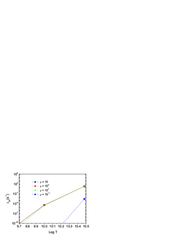
Figure 6: Positron captures on ⁵⁵Co as function of temperatures and densities. Densities in inset are in units of $gcm^{-3}$. Temperatures are measured in $K$.

For the parent nuclide we considered a maximum of 30 states. States still higher in excitation energy were not considered as their occupation probability was not high enough for the temperature and density scales chosen for this phase of core collapse. For each parent state we considered around 200 states of daughter. GT strength of each contributing state was taken into account. GT transitions are the dominant excitation mode for electron captures during the presupernova evolution. The B(GT) strength distributions for ground and two excited states at 2.2 MeV, and 2.6 MeV are shown in Figs. 1 and 2, respectively. We note that the GT strength is fragmented over many daughter states. For electron capture, the GT centroid resides in the energy range 7.1 and 7.4 MeV in the daughter ${}^{55}Fe$ and more or less in the energy range 6.7 - 7.5 MeV for both the excited states. We get a good energy resolution in our spectra which we attribute to the large model space. The corresponding values for the ground and the two excited states using shell model [28] are 6 MeV and 9 and 10 MeV, respectively, and are also shown by asterisk in the figure. We clearly see from Fig. 1 that our centroid is shifted to much lower energies for the excited states. Our code also calculated GT transitions for the states at 0.3 MeV and 0.4 MeV which are close lying states with the ground state. The centroids for these states are in the range of 6.6 and 7.4 MeV and 7.2 and 8.1 MeV, respectively. Transitions from these low-lying states contributed to the enhancement of our electron capture rates. For positron captures, the GT centroid resides at 9.1 MeV for the ground state. The corresponding values of the centroids for the 2.2 MeV and 2.6 MeV excited states are 9.2 MeV and 9.6 MeV, respectively. In some situations, the total GT strength is more important than the GT centroid. We worked out the total GT strength for the electron capture on ${}^{55}Co$ to be 7.4 and 17.9 for positron capture. The variation of electron capture rates for ${}^{55}Co$ with temperatures and densities is shown in Fig. 3. The temperature scale log T measures the temperature in K and the density shown in the inset has units of $gcm^{-3}$. In low density $(10-10^{4}gcm^{-3})$ regions of the star, the electron capture rates on ${}^{55}Co$ nuclide decreases as temperature of the stellar core increases. This trend continues until log T is in the vicinity of 8.6. Beyond this temperature electron capture rates shoots up. In low temperature regions (log T = 7.0), when the stellar core shift from densities $\rho=10^{7}gcm^{-3}$ to $10^{11}gcm^{-3}$, the electron capture rates are enhanced by as much as 7 order of magnitude. For high densities $(\rho=10^{11}gcm^{-3})$, the electron capture rates remain constant until around log T = 10. Above this temperature enhancement of the electron capture rates take place. The electron capture rates for different densities grid and temperatures can be seen from Table I.

Table 1: Electron Capture Rates ${}^{55}Co\longrightarrow^{55}Fe$

$\rho(gcm^{-3})$/logT	7	8.6	9.2	9.7	10.5
10	3.4(-8)	6.0(-9)	8.3(-6)	6.0(-3)	6.3(2)
$10^{4}$	1.2(-5)	5.8(-6)	1.2(-5)	6.1(-3)	6.3(2)
$10^{7}$	5.7(-3)	5.7(-3)	8.2(-3)	2.8(-2)	6.4(2)
$10^{11}$	4.7 (4)	4.7(4)	5.1(4)	5.9(4)	4.2(5)

Electron capture rates for ${}^{55}Co$ as function of temperature and density.
The values in the parenthesis represent the power of 10. The units of each rates are $sec^{-1}$.

The units of each rate are $sec^{-1}$. In Fig. 4 we compare our electron capture rates with that of Ref. [28]. Here $\rho_{7}$ measure the densities in $10^{7}gcm^{-3}$. We note that our rates are two orders of magnitude faster at low temperature as compared to Ref. [28]. Due to the complexity of the spectroscopy involved, authors in Ref. [28] had to switch to approximations like back resonances (the GT back resonance are states reached by the strong GT transitions in the electron capture process built on ground and excited states [6, 18]) and Brink’s hypothesis. The enhancement of our electron capture rates at presupernova temperatures is due to large GT+ transitions from the low-lying states of the parent nucleus. These states have finite probability of occupation at presupernova temperatures. We do not assume the Brink’s hypothesis. Our results show that the Brink’s hypothesis is a first order approximation and much of the times transitions from excited states are many orders of magnitude higher than those from the ground state [15]. Low-lying transitions are quite important at low temperatures and densities and supplement the electron capture rate from the GT resonance if the Q value only allows capture of high energy electrons from the tail of the Fermi- Dirac distribution. We see from the GT distribution (Fig. 1) that the GT centroid of the QRPA is very close to the shell model centroid, but our centroids for the excited states are at low energy in daughter as compared to shell model centroids. Contribution to rates from these states is many orders of magnitude larger than the ground state leading to an overall enhancement of our rates at low temperatures. At supernova temperatures the difference between the two calculations decreases. At higher temperatures and densities the energy of the electron is large compared to Q value for transitions to GT centroid. In such conditions the capture rates are no more dependent on the energy of the GT distribution but rather depend on the total GT strength [29]. The total GT strength of the QRPA, 7.4, is less than the shell model, 8.7. Our rates are still around four times faster than shell model ones at higher densities and temperatures ([see also Ref. [30]). We calculated a ${}^{55}Co$ halflife of 1108 sec. (18.74 hours), which is in good agreement with the experimental value of 17.53 hours [31]. FFN calculated stellar electron and positron capture rates for 226 nuclei with masses between A = 21 and 60. Measured nuclear level information and matrix elements available at that time were used and unmeasured matrix elements for allowed transitions were assigned an average value of log ft = 5. To complete the FFN rate estimate, the Gamow-Teller contribution to the rate was parameterized on the basis of the independent particle model and supplemented by a contribution simulating low-lying transitions. Fig. 5 shows the comparison of our rates with the FFN rates [6] for densities $\rho Y_{e}=10^{3}gcm^{-3}$ and $\rho Y_{e}=10^{11}gcm^{-3}$, respectively. For low densities $(\rho Y_{e}=10^{3}gcm^{-3})$ and temperatures our electron capture rates are enhanced by one order of magnitude than the FFN rates. Both rates increase with increasing temperature. We are in good agreement with the FFN when temperature of the stellar core is around log T = 9.4. Above this temperature, the FFN rates are enhanced than our rates. The enhancement in FFN rates become more pronounced at densities $\rho Y_{e}=10^{11}gcm^{-3}$. The main reason for this enhancement is the placement of the GT centroid at too low excitation energies by FFN as also pointed by authors in Ref. [28]. The competition between positron captures on neutrons and electron captures on protons is thought to play a crucial role in modeling of Type-II supernovae [19]. The positron captures are also of importance in stellar core having low density locations and enough high temperatures. The continuum positron capture and electron capture are characteristic of stellar plasma. Our positron capture rates are shown in Fig. 6. We note that around presupernova temperatures the positron capture rates are very slow as compared to the electron capture rates. We assumed in our calculations that positrons appear via electron-positron pair creation only when the stellar temperature exceeds 1 MeV. When the temperature of the stellar core increases further the positron capture rates shoot up. In high temperature regions of the stellar core, capture rates are more sensitive to the total GT strength distribution. We computed the total GT strength around 17.9. This results in high capture rates of positrons at low densities and high temperatures regions of stars. The positron capture rates decreases with increasing densities, in contrast to the electron capture rates which increase as density increases. As temperature rises, more and more positrons are created leading in turn to higher capture rates. Table II shows our calculations of positron capture rates (in units of $sec^{-1}$) at selected temperatures and densities.

Table 2: Positron Capture Rates ${}^{55}Co\longrightarrow^{55}Ni$

$\rho(gcm^{-3})$/logT	7	8.6	9.2	9.7	10.5
10	0.0	0.0	3.2(-33)	9.6 (-11)	1.9 (1)
$10^{4}$	0.0	0.0	2.2(-33)	9.5 (-11)	1.9 (1)
$10^{7}$	0.0	0.0	3.7(-37)	1.9 (-11)	1.9 (1)
$10^{11}$	0.0	0.0	0.0	7.6 (-35)	2.7 (-3)

Positron capture rates for ${}^{55}Co$ as function of temperature and density.
The values in the parenthesis represent the power of 10. The units of each rates are $sec^{-1}$.

V Summary

Electron and positron capture rates on ${}^{55}Co$ was calculated microscopically using the pn-QRPA theory, which has been used extensively for calculation of terrestrial weak rates with success. The pn-QRPA theory was used to calculate weak rates in stellar environment. This theory also gave us the liberty of using a large model space of $7\hbar\omega$. A total of 30 parent and around 200 daughter excited states for each parent state were considered in our calculations. For each pair of calculated parent and daughter states, the B(GT) strength was calculated in a microscopic fashion. ${}^{55}Co$ is considered a strong candidate among the other Fe peak nuclei that play a dominant role in electron capturing and hence in the core collapse of a star. At presupernova the dynamics of the star is very complex and large numbers of nuclear excited states are involved. The pn-QRPA is a judicious choice for handling these large numbers of excited states in heavy nuclei in the presupernova conditions of the stellar core. Our results point to a much more enhanced capture rate for ${}^{55}Co$ as compared to the reported shell model rates and can have a significant astrophysical impact on the core collapse simulations. The reduced capture rates for ${}^{55}Co$ in the outer layers of the core from the previous compilations resulted in slowing the collapse and posed a large shock radius to deal with [2]. What impact our enhanced rates may have on the core collapse simulations? According to Aufderheide et al. [19], the rate of change of lepton-to-baryon ratio ( $\dot{\psi{{}_{e}}}$ ) changes by about 50% alone due to electron capture on ${}^{55}Co$. Our results might point towards favoring a prompt explosion. One cannot conclude just on the basis of one kind of nucleus about the dynamics of explosion(prompt or delayed). We recall that it is the rate and abundance of particular specie of nucleus that prioritizes the importance of that particular nucleus in controlling the dynamics of late stages of stellar evolution.

References

- (1) H.A. Bethe, G.E. Brown, J. Applegate, and J.M. Lattimer, Nucl. Phys. A 324, 487 (1979).
- (2) W.R. Hix, O.E. Messer, A. Mezzacappa, M. Liebendrfer, J. Sampio, K. Langanke, D.J. Dean, and G. Martínez-Pinedo, Phys. Rev. Lett. 91, 201102 (2003).
- (3) F.K. Sutaria, A. Ray, J.A. Sheikh, and P. Ring, Astron. Astrophys. 349, 135 (1999).
- (4) A. Heger, N. Langer, S.E. Woosley, Ap. J. 528, 368 (2000).
- (5) H.A. Bethe, Rev. Mod. Phys. 62, 801 (1990).
- (6) G. M. Fuller, W. A. Fowler, and M. J. Newman, ApJS 42, 447 (1980); 48, 279 (1982); ApJ 252, 715 (1982).
- (7) M.B. Aufderheide, G.E. Brown, T.T.S. Kuo, D.B. Stout, and P. Vogel, ApJ362, 241 (1990).
- (8) C.W. Johnson, S.E. Koonin, G.H. Lang, and W.E. Ormand, Phys. Rev. Lett. 69, 3157 (1992).
- (9) S.E. Koonin, D.J. Dean, and K. Langange, Phys. Rep. 278, 1 (1996).
- (10) K. Langanke, G. Martinez-Pinedo, Rev. Mod. Phys. 75, 819 (2003).
- (11) J.-U. Nabi, H. V. Klapdor- Kleingrothaus, Atomic Data and Nuclear Data Tables 71, 149 (1999).
- (12) J. A. Halbleib, R. A. Sorensen, Nucl. Phys. A 98, 542 (1967).
- (13) J. Krumlinde, P. Muller, Nucl. Phys. A 417, 419 (1984).
- (14) P. Muller, J. Randrup, Nucl. Phys. A 514, 1 (1990).
- (15) J.-U. Nabi, H.V. Klapdor- Kleingrothaus, Atomic Data and Nuclear Data Tables 88, 237 (2004).
- (16) J.-U. Nabi, H. V. Klapdor- Kleingrothaus, Eur. Phys. J. A 5, 337 (1999).
- (17) J.-U. Nabi, Ph.D. Thesis, Heidelberg University Germany, 1999.
- (18) A. Heger, K. Langanke, G. Mart nez-Pinedo, and S.E. Woosley, Phys. Rev. Lett. 86, 1678 (2001).
- (19) M.B. Aufderheide, I. Fushiki, S.E. Woosley, E. Stanford, and D.H. Hartmann, Astrophys. J. Suppl. 91, 389 (1994).
- (20) S.G. Nilsson, Mat. Fys. Medd. Dan. Vid. Selsk 29, No.16 (1955).
- (21) A. Staudt, E. Bender, K. Muto, and H.V. Klapdor-Kleingrothaus, Atomic Data and Nuclear Data Tables 44, 79 (1990).
- (22) M. Hirsch, A. Staudt, K. Muto, and H.V. Klapdor-Kleingrothaus, Atomic Data and Nuclear Data Tables 53, 165 (1993).
- (23) I. Ragnarsson, R.K. Sheline, Phys. Scr. 29, 385 (1984).
- (24) M. Hirsch, A. Staudt, K. Muto, and H.V. Klapdor-Kleingrothaus, Nucl. Phys. A 535, 62 (1991).
- (25) N.B. Gove, M.J. Martin, Atomic Data and Nuclear Data Tables 10, 205 (1971).
- (26) K. Grotz, H.V. Klapdor, The Weak Interaction in Nuclear, Particle and Astrophysics, Adam Hilger, (IOP Publishing, Bristol, Philadelphia, New York, 1990).
- (27) K. Muto, E. Bender, and H.V. Klapdor- Kleingrothaus, Z. Phys. A 334, 187 (1989).
- (28) K. Langanke, G. Martinez-Pinedo, Phys. Lett. B 436, 19 (1998).
- (29) K. Langanke, G. Martinez-Pinedo, Nucl. Phys. A 673, 481 (2000).
- (30) J.-U. Nabi, M.-U. Rahman, Phys. Lett. B 612, 190 (2005).
- (31) G. Audi, O. Bersillon, J. Blachot, and A.H. Wapstra, Nucl. Phys. A 729, 3 (2003).