Studying the Dynamical Properties of 20 Nearby Galaxy Clusters

Abstract

Using SDSS-DR7, we construct a sample of 42382 galaxies with redshifts in the region of 20 galaxy clusters. Using two successive iterative methods, the adaptive kernel method and the spherical infall model, we obtained 3396 galaxies as members belonging to the studied sample. The 2D projected map for the distribution of the clusters members is introduced using the 2D adaptive kernel method to get the clusters centers. The cumulative surface number density profile for each cluster is fitted well with the generalized King model. The core radii of the clusters’ sample are found to vary from 0.18 Mpc $\mbox{h}^{-1}$ (A1459) to 0.47 Mpc $\mbox{h}^{-1}$ (A2670) with mean value of 0.295 Mpc $\mbox{h}^{-1}$.

The infall velocity profile is determined using two different models, Yahil approximation and Praton model. Yahil approximation is matched with the distribution of galaxies only in the outskirts (infall regions) of many clusters of the sample, while it is not matched with the distribution within the inner core of the clusters. Both Yahil approximation and Praton model are matched together in the infall region for about 9 clusters in the sample but they are completely unmatched for the clusters characterized by high central density. For these cluster, Yahil approximation is not matched with the distribution of galaxies, while Praton model can describe well the infall pattern of such clusters.

The integrated velocity dispersion profile shows that there are different behaviors within the cluster’s virialized region, while it exhibits a flattened out behavior outside the virialized region up to the turnaround radius. Under the assumption that the mass follows galaxy distribution, we determine the mass and mass profile by two independent mass estimators; projected mass and virial mass methods. The virial mass profile is corrected by applying the surface pressure term which reduces the virial mass by about $14\%$. The projected mass profile is larger than the corrected virial mass profile for nearly all clusters by about $28\%$. The virial mass agrees with NFW mass and Praton mass at $r_{v}$. The virial mass profile within 1.5 Mpc $\mbox{h}^{-1}$ is fitted with NFW mass profile. The concentration parameter ranges from $1.3$ to $39.17$, and has mean value $12.98$.

1 Introduction

Knowledge of physics of beginning, evolution, and fate of our universe requires understanding the distribution, formation, dynamics, and evolution of matter on a large scale. Galaxy clusters, which are the most massive gravitationally bound galaxy systems, play an important role in the study of the large-scale structure formation (Fadda et al. 1996; Girardi et al. 1998), as well as to understand the physics of the universe as a whole.

Studying the properties of galaxy clusters based on old catalogs is affected by the projection effect. New and deep redshift surveys (e.g. Sloan Digital Sky Survey, hereafter SDSS) for galaxies on nearly whole sky help to overcome such problem. However, the redshift information is distorted by some factors, e.g. small scale structure, large scale structure, and observational errors. This distortion leads to difficulty to determine the real cluster members which is the most important factor to study the dynamics of galaxy clusters. There are many methods used to get cluster members. Some of them are based on statistical rules and others are based on the dynamical status of the system. Enhanced methods were introduced in the last 2 decades to get the clusters members which take into account the distance from the cluster center beside the redshift information. However, no specific method introduces an accurate confirmation on the real cluster members.

The aims of this work are: (i) Determination of centers and members for 20 nearby galaxy clusters based on a two-steps method. (ii) Study the redshift space and the infall pattern around them. (iii) Study the integrated velocity dispersion profile. (iv) Investigation and determination of the clusters masses and mass profiles using two different mass estimators.

The paper is organized as follows. We describe the data sample in Sec. 2. The determination of the cluster center and the selection procedure for cluster membership assignment are described in Sec. 3. The density profiles of galaxy clusters are illustrated in Sec. 4. The spherical infall models; linear model, Yahil approximation and Praton model, are discussed in Sec. 5. The velocity dispersion profile and the effects influence it are described on Sec. 6. We briefly describe the methods used to compute cluster masses using member galaxies in Sec. 7. The clusters physical parameters and correlations between them are introduced in Sec. 8. We give a brief summary of our main results and draw our conclusions in Sec. 9.

2 Data Sample

We choose 20 nearby Abell clusters from Aguerri, Sańchez-Janssen & Münoz-Tünón 2007 (hereafter AG2007) and Yoon et al. (2008) (hereafter YO2008). Using photometric and spectroscopic data of objects classified as galaxies from the SDSS-DR7, we select only those galaxies with redshifts between $0.0<z<0.15$ around each galaxy cluster center selected from the two above references. The choice of the search radius around the center of each galaxy cluster depends on the value of the cluster redshift taken from AG20007 and YO2008. Data for each galaxy consists of right ascension ($\alpha$), declination ($\delta$), redshift, and magnitudes u, g, r, i, and z. Table 1 shows the results of the search. Col. 1 is the cluster name, col. 2 and 3 are $\alpha$ and $\delta$ of the center of the search, col. 4 is the radius of the search, and col. 5 is the number of galaxies found within the search radius. More details about SDSS-DR7 are described in Abazajian et al. 2009 and the website www.sdss.org.

Table 1: List of the galaxy clusters sample with the search radius and resultant number.

Name	$\alpha$ (deg)	$\delta$ (deg)	$\theta$	No.
	(2000)	(2000)	(arcmin)
A0117	14.0	-10.0	100	645
A0168	18.7	0.4	180	1296
A0671	127.1	30.4	120	996
A0779	140.0	33.8	300	4778
A1066	160.0	5.2	100	763
A1142	165.2	10.6	150	1708
A1205	168.3	2.5	100	890
A1238	170.7	1.1	100	830
A1377	176.9	55.8	150	2671
A1424	179.4	5.1	100	826
A1436	180.1	56.2	100	1130
A1459	181.1	1.9	300	5960
A1663	195.7	-2.6	100	721
A1767	204.0	59.2	120	1089
A1809	208.3	5.2	120	1170
A2048	228.8	4.4	100	1518
A2061	230.3	30.6	100	1365
A2142	239.6	27.2	120	1740
A2255	258.2	64.1	120	813
A2670	358.6	-10.4	100	502

3 Determination of the center and members of galaxy cluster

Dynamical parameters of galaxy clusters, such as mean cluster redshift, velocity dispersion, mass and virial and turnaround radii are significantly affected by the method of determination of the cluster center and the procedure of the membership selection. The methods used to get cluster center and members are illustrated in the following two subsections.

3.1 Cluster Center

The cluster center can be defined as, the position at which the surface luminosity is maximum. Depending on this definition the cluster center can be determined using either X-ray observation of inter-galactic gas settled in the cluster or optical observation of the galaxies themselves. The position of the maximum galaxy number per unit area indicates the maximum surface luminosity which by definition indicates the cluster center. Also one can define the cluster center as the dynamically oldest part of the cluster so the presence of a cD galaxy, giant elliptical galaxy (gE) or a central group of early type galaxies refers to the position of the cluster center (den Hartog & Katgert 1996).

In order to determine the cluster center we apply a non-parametric density estimator called the adaptive kernel method, hereafter AKM, (see Pisani 1993, Pisani 1996, Fadda et al. 1998) to get separately the maximum probability in $\alpha$, $\delta$, and $z$ directions. Then, the galaxy closest to the maximum probability is considered as the cluster center and referred to as the reference galaxy.

3.2 Membership Determination

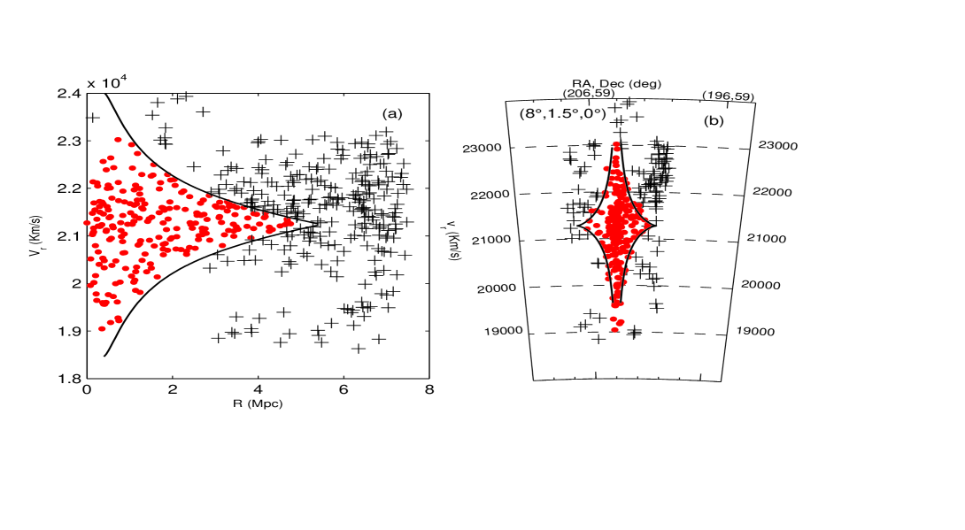
Figure 1: The distribution of galaxies of A1767 in $\mbox{S}_{p}$ (panel a) and $\mbox{S}_{v}$ (panel b), respectively. The two curves in each space indicate the application of SIM.

Several methods have been developed in order to obtain reliable members of galaxy cluster and to avoid the presence of interlopers. These methods can be classified into two families. First, those algorithms that use only the redshift information, e.g. 3$\sigma$-clipping techniques (Yahil & Vidal 1977), fixed gapping procedures (Beers, Flynn& Gebhardt 1990, Zabludoff et al. 1990), and jackknife technique (Perea et al. 1990). These methods are based on statistical rules. The other family uses information of both position and redshift, such as the shifting gap procedure designed by Fadda et al. (1996) or methods designed by den Hartog & Katgert (1996), or Regos & Geller (1989), which are based on physical rules.

To determine cluster members we use a two-steps method which is described as the following:

1. Redshift Information: AKM is used to find the significant peaks in the redshift distribution. For each iteration we choose a cut-off range that is selected manually outside the main peak to secure the conservation of the galaxy cluster members. The iteration is stopped when one single-peak is observed within the new cut-off range.

2. Redshift-Distance Information: Galaxies belonging to the main peak are analyzed in the second step, in which we use the combination of the projected distance from the cluster center and redshift information. The method used for this purpose is the spherical infall model, hereafter SIM (see Sec. 5). After applying SIM one can get the limits of the infall velocity that galaxies would have within the cluster as a function of distance from its center. Any galaxy outside this limits is classified as an interloper. This method is iterated until no more galaxies are excluded. The important advantages of this method are it takes combined radial velocity-space information into account and the removing of outliers is based on physical rules. The disadvantage of this method is that it is not valid inside or near the virialized region (see e.g. Regos & Geller 1989).

Using the redshift space (peculiar velocity versus projected distance from the cluster center, hereafter $\mbox{S}_{p}$), van Haarlem et al. (1993) conclude that Coma cluster is too elongated to be described by SIM. Also, Diaferio & Geller (1997) say that SIM is not good to describe the infall region of galaxy clusters due to random motions (substructures and/or recent mergers). Figure (1.a) shows $\mbox{S}_{p}$ for A1767 which describes this problem. As shown, although there are some galaxies (pluses) that should be included to the cluster according to Diaferio technique (see Figure 5 in Rines & Diaferio 2006 for A1767), SIM (the two curves) does not include them. Another redshift space, called cone diagram or slice oriented around the cluster center ($\alpha=204^{\circ}$ and $\delta=59^{\circ}$) with length = $8^{\circ}$ and width = $1.5^{\circ}$ (see Praton & Schneider 1994), hereafter $\mbox{S}_{v}$, is shown in Figure (1.b). This figure shows that these galaxies (pluses) which seem to belong to the cluster in $\mbox{S}_{p}$ are far from the cluster in $\mbox{S}_{v}$ and this is due to the projection effect. The application of SIM in $\mbox{S}_{v}$ (see Praton 1993) shows that the galaxies which are considered to be outliers in $\mbox{S}_{p}$ are also far and not included within the model in $\mbox{S}_{v}$. Because of that and with avoiding the effect of substructure for the studied clusters (see Figure 3), we depend on SIM to get the cluster members in $\mbox{S}_{p}$.

As illustrated, we determine clusters’ members using the two-steps method, AKM (first step) and SIM (second step). We depend on Yahil approximation (see Sec. 5) which requires determination of the density contrast profile, $\Delta(\leq R)$, of the cluster, the background density, $\rho_{bg}$, and the cosmological parameter, $\Omega_{0}$. We select $\Omega_{0}=1$ and $\mbox{H}_{0}=100\mbox{ Km s}^{-1}\mbox{ Mpc}^{-1}$. The distance to a cluster center is calculated using $D=cz_{cl}/H_{0}$, where $z_{cl}$ is the average redshift of the cluster’s members. Table 2 shows the results of determination of the cluster members after applying these two steps, respectively.

Table 2: The number of the cluster members after applying the one dimensional AKM (the first step) and SIM (the second step).

	First Step				Second Step
	(AKM)				(SIM)
Name	$z_{min}$	$z_{max}$	No.		$z_{min}$	$z_{max}$	No.
A0117	0.047	0.060	221		0.049	0.059	146
A0168	0.037	0.053	322		0.039	0.050	194
A0671	0.045	0.057	216		0.046	0.057	162
A0779	0.018	0.031	500		0.019	0.031	191
A1066	0.061	0.079	291		0.063	0.075	160
A1142	0.028	0.040	223		0.031	0.039	122
A1205	0.067	0.089	316		0.072	0.080	93
A1238	0.065	0.078	190		0.070	0.078	85
A1377	0.048	0.055	353		0.048	0.055	158
A1424	0.069	0.082	313		0.071	0.080	94
A1436	0.058	0.071	278		0.059	0.070	142
A1459	0.015	0.025	284		0.016	0.025	189
A1636	0.077	0.094	428		0.079	0.089	110
A1767	0.062	0.081	511		0.064	0.077	226
A1809	0.074	0.087	418		0.075	0.085	125
A2048	0.086	0.109	401		0.092	0.103	90
A2061	0.067	0.089	486		0.071	0.083	228
A2142	0.084	0.100	746		0.084	0.098	419
A2255	0.072	0.087	439		0.073	0.087	279
A2670	0.068	0.085	309		0.070	0.082	183

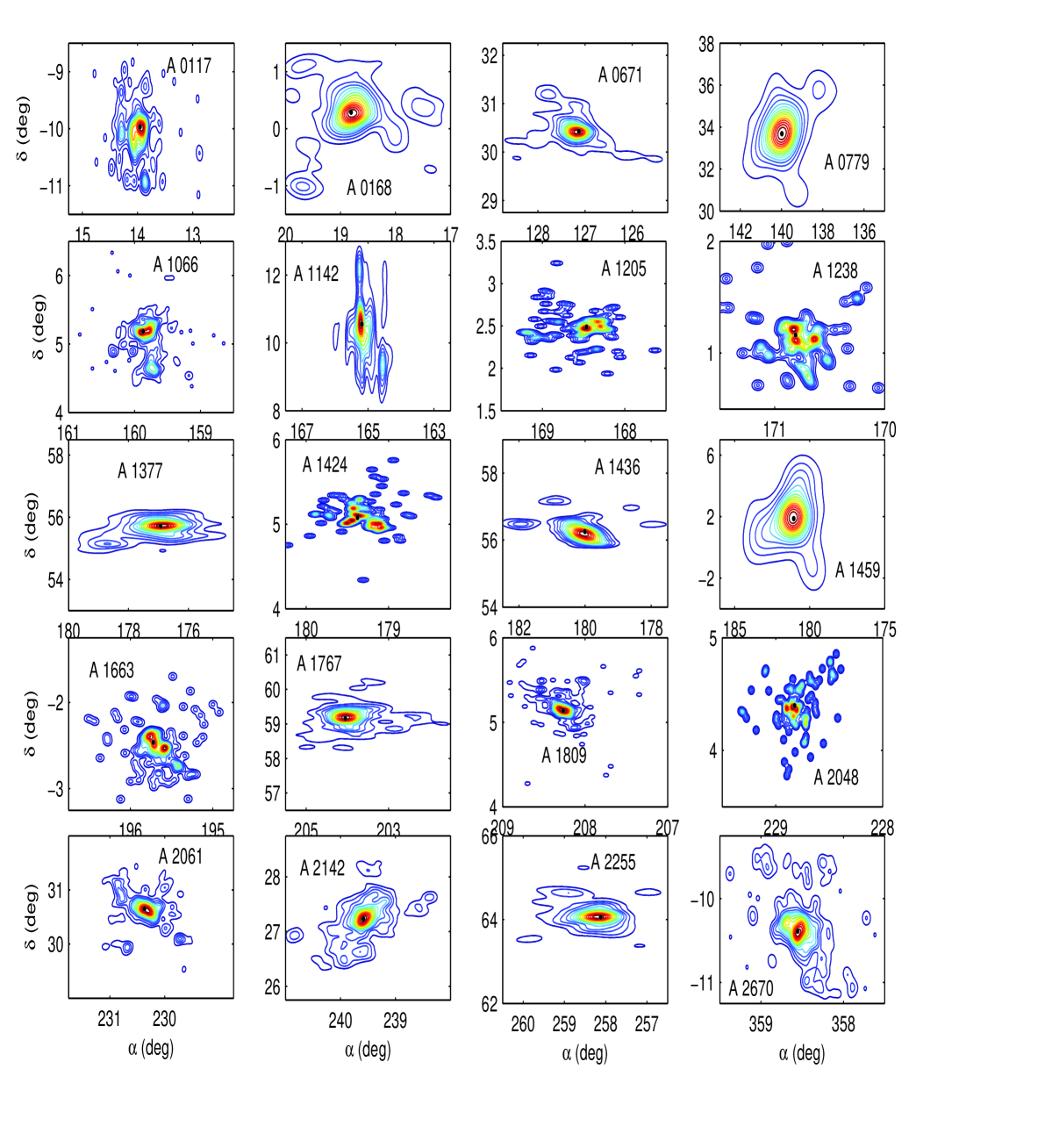
Figure 2: Adaptive-kernel contour map (20 levels) of surface number density. Filled circle represents the galaxy cluster center.

The center of each cluster is obtained using the two dimensional AKM applied to $\alpha$ and $\delta$ beside the one dimensional AKM applied to $z$ for the galaxies considered as cluster members. Figure 2 shows the isodensity contour maps for the distribution of the cluster members. The four clusters A0168, A0671, A0779 and A1459 exhibit smooth distributions of galaxies without substructure in the projected map, while the other clusters show non-regularity in the isodensity map distribution and some of them show presence of substructures in their projected maps.

Figure 3 shows the redshift distribution for galaxy members in each cluster. We find that most clusters appear as a well isolated peak in the redshift space and represent Gaussian distribution. This means that there are no substructures in the redshift space within these clusters, although in the projected map some of them show presence of substructure.

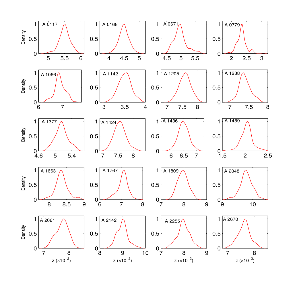
Figure 3: Redshift distribution of galaxies in each cluster of the studied sample.

It is found that there are projection overlaps between the two clusters A1377 and A1436 and the two clusters A1424 and A1459. To avoid duplication of any member among such overlapped clusters, we explore them in redshift space, see Figure 4. The two clusters A1377 and A1436 are plotted in the redshift space relative to A1377 center and the redshift space of the two clusters A1424 and A1459 is drawn relative to A1459 center. Although the sky map (Figure 4 left panels) of the members of each cluster pairs shows overlapping, the redshift space map (Figure 4 right panels) shows that the clusters in each pair are separate.

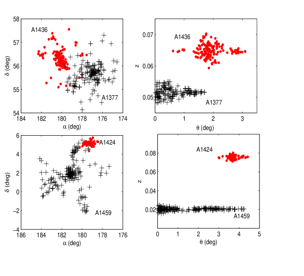
Figure 4: Sky position (left panels) and redshift space (right panels) for the clusters appearing overlapped: clusters A1377 (asterisk) and A1436 (point) (upper panels) and clusters A1424 (point) and 1459 (asterisk) (lower panels).

Table 3 shows the basic parameters of each cluster. Cols. 2-4 give the cluster center using AKM, cols. 5-7 give the coordinates of the reference galaxy, col. 8 gives the mean redshift of the cluster, and cols. 9-11, and 12-14 give $\alpha$, $\delta$, and $<z>$ for AG2007 and YO2008, respectively (see also Rines et al. 2006). It is clear that the clusters centers obtained by this study are very close to those work.

Table 3: The basic parameters of the clusters in the studied sample with comparison with other studies.

	AKM				Ref. Galaxy				AG2007				YO2008
Name	$\alpha$(deg)	$\delta$(deg)	z		$\alpha$ (deg)	$\delta$ (deg)	z	$<z>$	$\alpha$ (deg)	$\delta$ (deg)	$<z>$		$\alpha$ (deg)	$\delta$ (deg)	$<z>$
A0117	13.96	-10.02	0.055		13.96	-9.97	0.055	0.055	14.01	-10.00	0.055		14.08	-10.00	0.055
A0168	18.79	0.28	0.045		18.81	0.29	0.046	0.045	18.74	0.37	0.045		-	-	-
A0671	127.17	30.41	0.050		127.13	30.43	0.050	0.050	127.12	30.42	0.049		127.13	30.41	0.051
A0779	139.95	33.68	0.023		139.99	33.68	0.023	0.023	139.96	33.77	0.023		-	-	-
A1066	159.77	5.19	0.068		159.87	5.18	0.068	0.069	159.91	5.174	0.069		159.77	5.21	0.069
A1142	165.21	10.44	0.035		165.19	10.55	0.034	0.035	165.22	10.55	0.035		-	-	-
A1205	168.41	2.47	0.076		168.46	2.49	0.073	0.076	168.32	2.54	0.076		168.33	2.54	0.076
A1238	170.77	1.11	0.073		170.81	1.16	0.073	0.074	170.71	1.09	0.074		-	-	-
A1377	176.88	55.72	0.051		176.93	55.71	0.051	0.052	176.88	55.76	0.051		176.81	55.72	0.052
A1424	179.34	5.06	0.076		179.38	5.08	0.076	0.075	179.36	5.12	0.076		179.37	5.09	0.076
A1436	180.03	56.21	0.065		180.00	56.26	0.067	0.065	180.09	56.23	0.065		180.06	56.26	0.064
A1459	181.06	1.86	0.021		181.06	1.87	0.021	0.020	181.10	1.88	0.020		-	-	-
A1663	195.69	-2.49	0.083		195.72	-2.46	0.080	0.084	195.71	-2.52	0.083		195.72	-2.41	0.084
A1767	204.03	59.21	0.071		204.05	59.16	0.071	0.071	204.02	59.20	0.071		204.03	59.21	0.071
A1809	208.26	5.15	0.080		208.27	5.14	0.079	0.080	208.24	5.16	0.079		208.26	5.14	0.080
A2048	228.83	4.34	0.098		228.82	4.40	0.098	0.098	-	-	-		228.81	4.38	0.098
A2061	230.34	30.65	0.078		230.37	30.65	0.079	0.077	230.31	30.61	0.079		230.33	30.67	0.079
A2142	239.58	27.26	0.090		239.58	27.23	0.091	0.090	-	-	-		239.58	27.23	0.090
A2255	258.17	64.07	0.080		258.12	64.06	0.073	0.080	258.22	64.07	0.080		258.20	64.05	0.083
A2670	358.52	-10.36	0.077		358.56	-10.39	0.079	0.076	358.55	-10.41	0.076		358.55	-10.39	0.076

4 Density Profiles of Galaxy Clusters

The number density profile of galaxy clusters is introduced by some authors to describe the surface distribution of galaxies in clusters. King (1966, 1972) introduced an analytical representation of the galaxy distribution profile in clusters. This profile was devised to describe the surface brightness distributions in globular clusters and in elliptical galaxies, but it can also be applied to galaxy clusters (Bahcall 1977). The generalized King profile is given by

$$\Sigma(<R)=\Sigma_{0}\left(1+\frac{R^{2}}{r_{c}^{2}}\right)^{\gamma}+\Sigma_{bg}$$ (1)

where $\Sigma_{0}$ is the central number density per unit area, $r_{c}$ is the core radius, $\gamma$ is a power parameter and $\Sigma_{bg}$ is the background surface number density of the universe (Adami et al. 1998). The corresponding spatial density profile, using Abel integral, is given by

$$\rho(<r)=\rho_{0}\left(1+\frac{r^{2}}{r_{c}^{2}}\right)^{(\gamma-0.5)}+\rho_{bg},$$ (2)

$$\rho_{0}=\frac{\Gamma(0.5-\gamma)}{\Gamma(0.5)\Gamma(-\gamma)}\frac{\Sigma_{o}}{r_{c}}$$ (3)

(Regos & Geller 1989 and Van Haarlem et al. 1993). Note that $\rho_{0}$ is the central number density per unit volume and $\rho_{bg}$ is the background volume number density of the universe.

The background density, $\rho_{bg}$, can be obtained by integrating the Schechter luminosity function (Schechter 1976) and its corresponding magnitude function, $\Phi(M)$, where

$$\begin{split}\Phi(M)dM&=0.921N^{*}\left(10^{0.4(\alpha+1)(M^{*}-M)}\right)\times\\ &\quad\exp\left(-10^{0.4(M^{*}-M)}\right)dM,\end{split}$$ (4)

$$\begin{split}\rho_{bg}&=\int_{-\infty}^{M_{lim}}\Phi(M)dM\\ &\quad=0.921N^{*}\Gamma\left(\alpha+1,10^{0.4(M^{*}-M_{lim}+5\log D+25)}\right)\end{split}$$ (5)

where $M_{lim}$ is the limiting apparent magnitude of the survey and $D$ is the distance to the cluster center in Mpc (Regos & Geller 1989). The three parameters $N^{*}$, $M^{*}$ and $\alpha$ are determined for the the survey using Schechter luminosity function. We choose $N^{*}=0.0468\mbox{ h}^{3}\mbox{ Mpc}^{-3}$, $M^{*}=-18.24+5\log_{10}\mbox{h}$, $\alpha=-1.31$ for $u$ band with cosmological parameters $\Omega_{m}=1.0$ and $\Omega_{\Lambda}=0.0$ (Blanton 2001).

The mass density profiles of galaxy clusters are introduced by several authors. Navarro et al. (1995, 1996, 1997, hereafter NFW), and Hernquist 1990 propose two-parameter models based on Cold Dark Matter (CDM) simulations of haloes. The mass density profile introduced by NFW is given by

$$\rho(r)=\frac{\delta_{s}\rho_{s}}{\frac{r}{r_{s}}\left(1+\frac{r}{r_{s}}\right)^{2}},$$ (6)

and its corresponding mass profile is given by

$$M(<r)=\frac{M_{s}}{\ln(2)-(1/2)}\left[ln(1+\frac{r}{r_{s}})-\frac{r/r_{s}}{1+r/r_{s}}\right]$$ (7)

where $r_{s}$ is the scale radius, $M_{s}=4\pi\delta_{s}\rho_{s}r^{3}_{s}[\ln(2)-(1/2)]$ is the mass within $r_{s}$, and $\delta_{s}$ is the characteristic density (see Koranyi & Geller 2000, Rines et al. 2003).

The observed cumulative surface number density is fitted with the generalized King model (Eq. 1) using the Curve Fitting MatLab Toolbox. The parameters obtained from the fit are listed in Table 4. Col. 2 gives the cluster core radius, $r_{c}$, col. 3 gives the central surface number density, $\Sigma_{0}$, and col. 4 gives the value of $\gamma$. The standard error for each fitted parameter is with $95\%$ confidence level. Col. 5 gives the adjusted R-square to indicate the goodness of fit (see MatLab help for the goodness of fit). The adjusted R-square statistic can take on any value less than or equal to 1, with a value closer to 1 indicating a better fit.The core radius, $r_{c}$, has mean value of 0.295 Mpc $\mbox{h}^{-1}$ and range from 0.18 Mpc $\mbox{h}^{-1}$ (A1459) to 0.47 Mpc $\mbox{h}^{-1}$ (A2670). While $\Sigma_{0}$ has mean value 146.29 Mpc^-2 $\mbox{h}^{2}$ and range from 53.6 Mpc^-2 $\mbox{h}^{2}$ (A1424) to 411.8 Mpc^-2 $\mbox{h}^{2}$ (A1459). Notice that the two clusters A0779 and A1459 are characterized by high central surface densities.

Figure 5 shows the cumulative surface number density profile (dotted curve) fitted with the generalized King model (solid line). The two vertical solid and dashed lines represent the core and virial radii (see Sec. 5), respectively. The density decreases rapidly within the central regions and then decreases slowly until reaching the boundary of the cluster.

Table 4: Fitted parameters for the King model.

Name	$r_{c}$	$\Sigma_{0}$	$\gamma$	R-Square
	(Mpc/h)	(h2/Mpc2)
A0117	0.27$\pm$0.03	122 $\pm$ 6	-0.68 $\pm$0.03	0.999 $\pm$ 0
A0168	0.19$\pm$0.07	223 $\pm$ 49	-0.65 $\pm$0.06	0.996 $\pm$ 0.001
A0671	0.28$\pm$0.02	205 $\pm$ 8	-0.79 $\pm$0.03	0.999 $\pm$ 0
A0779	0.20$\pm$0.03	276 $\pm$ 24	-0.70 $\pm$0.03	0.999 $\pm$ 0
A1066	0.24$\pm$0.04	173 $\pm$ 17	-0.69 $\pm$0.04	0.998 $\pm$ 0.001
A1142	0.26$\pm$0.06	111 $\pm$ 14	-0.68 $\pm$0.07	0.997 $\pm$ 0.001
A1205	0.21$\pm$0.03	100 $\pm$ 10	-0.63 $\pm$0.03	0.999 $\pm$ 0
A1238	0.32$\pm$0.12	63 $\pm$ 10	-0.65 $\pm$0.12	0.991 $\pm$ 0.004
A1377	0.20$\pm$0.04	182 $\pm$ 26	-0.67 $\pm$0.04	0.998 $\pm$ 0.001
A1424	0.36$\pm$0.12	54 $\pm$ 7	-0.62 $\pm$0.11	0.988 $\pm$ 0.005
A1436	0.26$\pm$0.11	100 $\pm$ 21	-0.61 $\pm$0.10	0.999 $\pm$ 0
A1459	0.18$\pm$0.02	412 $\pm$ 35	-0.77 $\pm$0.02	0.999 $\pm$ 0
A1663	0.35$\pm$0.10	64 $\pm$ 7	-0.66 $\pm$0.10	0.992 $\pm$ 0.003
A1767	0.31$\pm$0.02	137 $\pm$ 3	-0.67 $\pm$0.02	0.999 $\pm$ 0
A1809	0.32$\pm$0.02	151 $\pm$ 5	-0.81 $\pm$0.03	0.999 $\pm$ 0
A2048	0.30$\pm$0.10	65 $\pm$ 10	-0.62 $\pm$0.09	0.994 $\pm$ 0.002
A2061	0.44$\pm$0.03	111 $\pm$ 3	-0.73 $\pm$0.03	0.999 $\pm$ 0
A2142	0.45$\pm$0.03	102 $\pm$ 3	-0.62 $\pm$0.02	0.999 $\pm$ 0
A2255	0.28$\pm$0.04	189 $\pm$ 12	-0.66 $\pm$0.04	0.998 $\pm$ 0.001
A2670	0.47$\pm$0.08	84 $\pm$ 5	-0.73 $\pm$0.08	0.996 $\pm$ 0.001

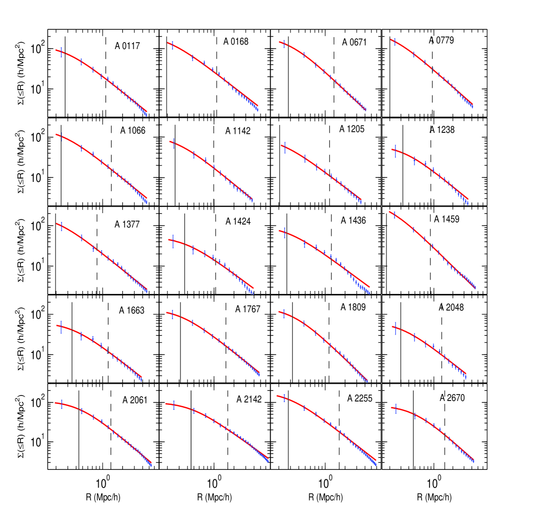
Figure 5: The cumulative surface number density profiles (dots) together with the generalized King model (solid line). The two vertical solid and dashed lines are $r_{c}$ and $r_{v}$, respectively.

5 Spherical Infall Model

Before describing SIM we describe galaxy clusters themselves. Galaxy clusters can be divided into two regions: inner virialized region and outer infall one. A virialized region is the region in which the system is in dynamical equilibrium, and the limit of this region is the virial radius, $r_{v}$. This radius can be defined as, the radius within which the density is 200 times the critical density of the universe (Carlberg, Yee & Ellingson 1997). The virialized region is surrounded by infall region in which the galaxies are falling into the gravitational potential well of the cluster, and they have not yet reached equilibrium (Rines et al. 2003).

SIM has been extensively described in literature (Gunn & Gott 1972, Silk 1974, Peebles 1976, Schechter 1980, Vedel & Hartwick 1998). It assumes that galaxy clusters started as small density perturbations in the early universe. These perturbations eventually deviate from the general Hubble flow of the universe and after reaching a maximum radius, i.e. its turnaround radius, they start collapsing. SIM describes the dynamics of the non-equilibrium region of galaxy clusters where the effects of virialization and crossing shells are negligible. Under the spherical symmetry assumption, the infall motion produces a pattern of caustic shape in the galaxy cluster redshift space. This pattern envelops all galaxies whose infall motion overwhelms the Hubble flow (Kaiser 1987).

Under the assumption of spherical symmetry, the cluster mass distribution can be considered as a set of concentric mass shells, whose centers coincide with that of the density perturbation and only the mass inside a shell influences the evolution of that shell, i.e. no mass transformation between shells. Hence each mass shell can be considered as an independently evolving Friedmann universe, characterized by the density inside it (den Hartog & Katgert 1996). Consequently, any shell enclosing density greater than the critical density will expand to a certain radius and then infall toward the cluster. In the frame of the cluster the infall velocity can be defined as

$$v_{inf}(r)=H_{0}r+v_{pec}(r)$$ (8)

where $v_{pec}$ is the peculiar velocity (see Sec. 6), and $\mbox{H}_{0}$ is the present value of the Hubble parameter (Regos & Geller 1989). Accordingly, the turnaround radius, $r_{t}$, for each shell can be defined as the radius at which the peculiar velocity of that shell exactly cancels the Hubble expansion, so that the material at this shell is physically standing still with respect to the cluster (Praton & Schneider 1994)

The linear theory of density perturbations shows that a spherically symmetric mass concentration in an expanding universe induces a radial peculiar velocity field in the surrounding region (see Gunn 1978, Peebles 1980)

$$\frac{v_{pec}}{H_{0}r}=-\frac{1}{3}\Omega_{0}^{0.6}\Delta(<r)$$ (9)

where $\Delta(<r)$ is the density contrast within radius $r$ which is defined as

$$\Delta(<r)=\frac{\rho(<r)}{\rho_{bg}}-1=\frac{\rho(<r)}{\Omega_{0}\rho_{c}}-1$$ (10)

where $\rho_{c}$ is the critical density of the universe and $\Omega_{0}$ is the cosmological density parameter.

To describe the peculiar velocity pattern around galaxy clusters, Yahil (1985) introduced the following non-linear approximation

$$\frac{v_{pec}(r)}{H_{0}r}=-\frac{1}{3}\Omega_{0}^{0.6}\frac{\Delta(<r)}{(1+\Delta(<r))^{0.25}}$$ (11)

As a result, one can get the infall velocity profile, $v_{inf}(r)$, for a cluster as

$$\frac{v_{inf}(r)}{H_{0}r}=1-\frac{1}{3}\Omega_{0}^{0.6}\frac{\Delta(<r)}{(1+\Delta(<r))^{0.25}}$$ (12)

The density contrast profile can be obtained by two different ways. The first way is to obtain $\Delta(<r)$ from the spatial number density profile of the cluster and the background number density of the universe. The second way is to determine the mass density profile of the cluster and the background mass density of the universe using $\rho_{bg}=\Omega_{0}\rho_{c}$ (van Haarlem et al. 1993).

The value of the density contrast at the turnaround radius can be derived using Eq. 12 where $v_{inf}=0$. Accordingly, $\Delta(r=r_{t})\approx 4.62$ for $\Omega_{0}=1$.

Einstein and Straus (1945, 1946) determined the metric of space-time near a star embedded in an expanding universe without a cosmological constant within general relativity. They assumed a star of mass $M$ is surrounded by an empty spherical cavity, called Einstein-Straus vacuole, with a radius, $r_{ES}$, defined as

$$r_{ES}=\left(\frac{3M}{4\pi\rho_{bg}}\right)^{1/3}$$ (13)

From the definition of the Einstein-Straus vacuole, it can be considered that $r_{ES}=r_{t}$ (for more details see Bonnor 1987, Plaga 2005). Therefore, one can calculate $r_{ES}$ theoretically by knowing the cluster mass.

Praton & Schneider (1994) presented a model to predict the infall velocity profile based on spherical accretion onto a central mass seed, $m_{c}$, in an otherwise uniform and expanding universe (see, e.g., Peebles 1980). Consider the material surrounding $m_{c}$ to be divided into nested spherical shells in which each shell is labeled by a parameter $\phi$, which is the the development angle of the Friedmann model (Regos & Geller 1989). The larger $\phi$ is, the closer the shell lies to the cluster. For bound or collapsed shells, $\phi$ is positive and for unbound shells, $\phi$ is negative. The equations of motion for these shells is

$$r(\phi)=r_{v}\left[\frac{M(\phi)}{M_{v}}\right]^{1/3}\left[\frac{3\pi/2+1}{\phi-\sin(\phi)}\right]^{2/3}\left|1-\cos(\phi)\right|,$$ (14)

$$\frac{dr}{dt}(\phi)=\pm\sqrt{3}\sigma_{v}\left[\frac{M(\phi)/M_{v}}{r(\phi)/r_{v}}\right]^{1/2}(1+cos(\phi))^{1/2},$$ (15)

where the negative sign is for $\phi<0$

$$\frac{M(\phi)}{M_{v}}=\frac{f(\Omega_{0})^{2/3}+(3\pi/2+1)^{2/3}}{f(\Omega_{0})^{2/3}\pm[\phi-\sin(\phi)]^{2/3}},$$ (16)

$$f(\Omega_{0})\equiv 2\frac{\sqrt{1-\Omega_{0}}}{\Omega_{0}}-\cosh^{-1}\left(\frac{2-\Omega_{0}}{\Omega_{0}}\right),$$ (17)

where $\sigma_{v}$ is the line of sight velocity dispersion of the cluster at $r_{v}$.

Praton model can be applied if one have the turnaround radius and the line of sight velocity dispersion of a cluster. Although $r_{v}$ in the Praton model is somewhat arbitrary or ad hoc we apply the Praton model for $\Omega_{o}=1$ after getting $r_{v}$ and $\sigma_{v}$ observationally. This is because $r_{v}$ is easier to get from observation.

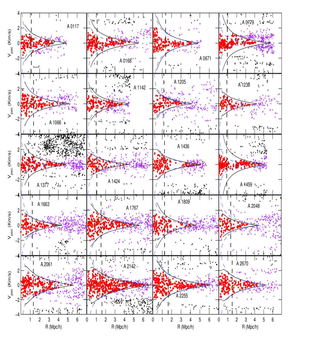
Figure 6: Distribution of galaxies in redshift space. The filled points indicate the cluster members. The plus and cross symbols indicate the interlopers obtained by AKM and SIM, respectively. The solid curved lines are the location of the caustics using Yahil model. The dashed curved lines indicate the location of the caustics using Praton model. The vertical dashed line indicates $r_{v}$.

Figure 6 shows the distribution of galaxies in the redshift space for each galaxy cluster. The filled points indicate the cluster members. The plus and the cross symbols refer to the interlopers obtained by AKM (first step) and interlopers obtained by the SIM (second step), respectively. The solid curved lines indicate the location of the caustics using Yahil model. The dashed curved lines indicate the location of the caustics obtained by Praton model for $r_{v}$. As mentioned before, we used Yahil approximation to determine the cluster members and the turnaround radius.

Yahil Approximation does not describe clusters’ virialized regions because of the assumption of conservation of mass is not valid within the cluster core due to the crossing shells where there are mass transfer inside the virialized region. Notice that Yahil approximation and Praton model are nearly coincide for the clusters A0671, A1066, A1205, A1424, A1436, A1663, A1767, A2255, and A2670. Also, Yahil approximation is enclosed within the Praton model for only A2048, while Praton model is enclosed and/or matched with Yahil approximation for A0117, A1142, A1238, A1809, and A2061. Finally both models are unmatched at all for A0168, A0779, A1377, and A1459.

For the two clusters A0779 and A1459, which are characterized by high central densities, Yahil approximation fails to describe their infall velocity profiles. In other words, the caustic boundaries of these two clusters are large in comparison with the distribution of their members within the virialized region. On the other hand, Praton model describes the infall velocity profiles for these two clusters with good acceptance. The two clusters A1436 and A1809 have nearly two empty regions between approximately $2-3.2$ and $\geq 2$, respectively. This may cause an overestimate in determination of the turnaround radii for these two clusters.

6 Velocity Dispersion Profile

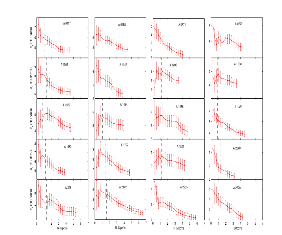
Figure 7: The Integrated velocity dispersion profile where the dispersion at a given radius is the average velocity dispersion within that radius. The vertical dashed line indicates the virial radius obtained by the corrected virial mass estimator.

The velocity dispersion profile, hereafter VDP, of a galaxy cluster is a measure of the cluster’s dynamical state and is considered as the most important ingredient for the calculation of different mass estimators and mass profiles.

For each galaxy the factor $(1+z_{obs})$, with $z_{obs}$ is the observed redshift of the galaxy, is the product of a factor $(1+z_{cl})$, which is due to the cosmological redshift, and $(1+z_{gal})$, which is the Doppler term due to the velocity of the galaxy with respect to the cluster center, where $z_{cl}$ is the cluster redshift and $z_{gal}$ is galaxy redshift with respect to the cluster center (Harrison & Noonan 1979, Danese, De Zotti & de Tullio 1980).

$$(1+z_{obs})=(1+z_{cl})(1+z_{gal})$$ (18)

Therefore, the peculiar velocities (or the velocity dispersions) of galaxies in the frame of the cluster, taking into account the correction for cosmological redshift, are computed as

$$v_{pec}=\frac{c(z_{obs}-z_{cl})}{(1+z_{cl})}$$ (19)

den Hartog & Katgert (1996) classified VDPs into three kinds; peaked, which deceases with the distance from the cluster center, flat, and inverted, which increases with the distance from the cluster center. The differences in VDPs are due to several factors like cluster member selection, choice of the cluster center, possible velocity anisotropies in galaxy orbits, presence of substructure and the presence of a population of spiral galaxies not in virial equilibrium with the cluster potential or the projection effect. Also, VDP may be influenced by the existence of other structures on larger scales such as a nearby cluster or the super-cluster, to which the cluster belongs, or filament and so on (see den Hartog & Katgert 1996, Girardi et al. 1996, Fadda et al. 1996).

Possible velocity anisotropies affect the shape of VDP, particularly within the central regions of the clusters. In order to avoid effects of possible anisotropies on the total value of velocity dispersion, Girardi et al. (1996) suggested studying the integral velocity dispersion profile (hereafter IVDP), where the dispersion at a given radius is evaluated by using all the galaxies within that radius. Although the presence of velocity anisotropies can strongly influence the value of integral velocity dispersion $\sigma$ computed for the central cluster region, it does not affect the value of the spatial (or projected) $\sigma$ computed for the whole cluster (The & White 1986, Merritt 1988).

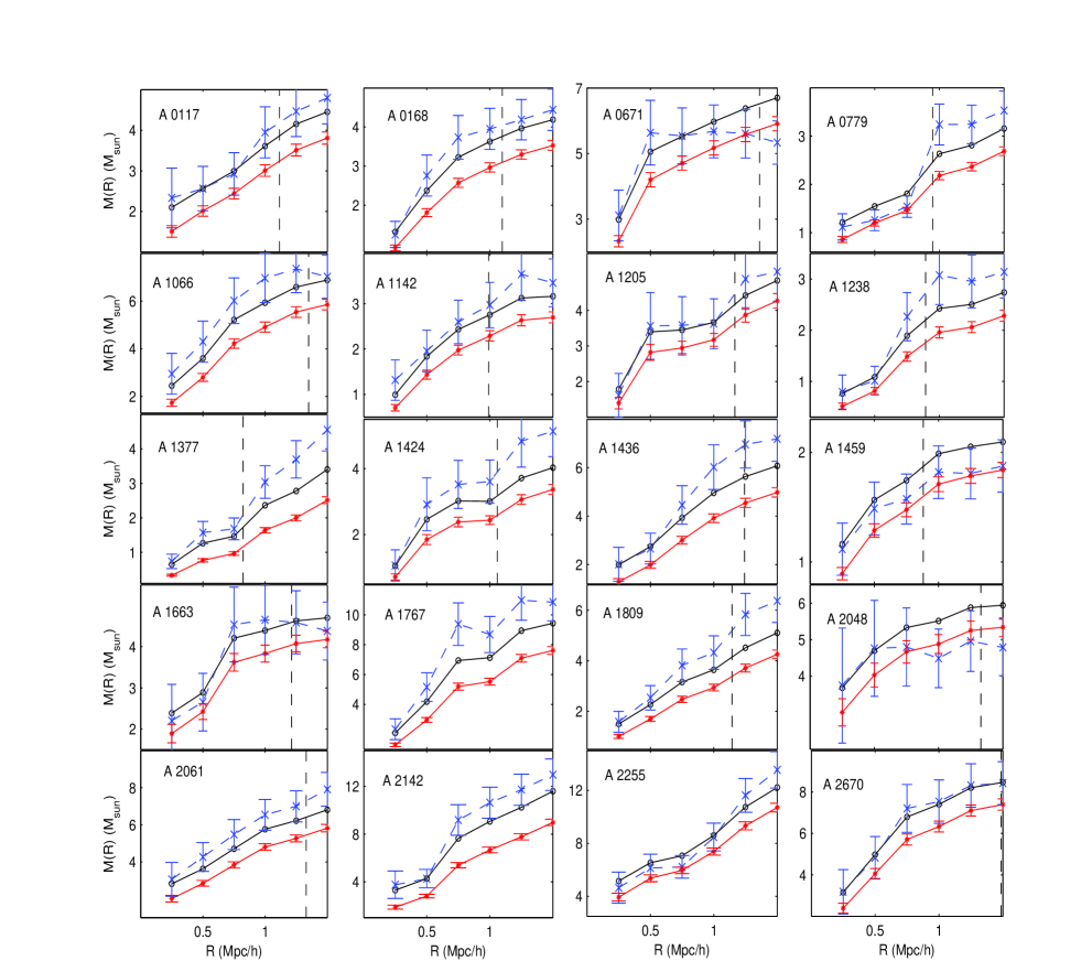
Figure 8: The cluster mass profiles obtained using different mass estimators. The open circle and dotted lines are the virial mass profile before and after correction respectively. The cross line represents the mass profile obtained using the isotropic projected mass estimator. The vertical dashed line indicates the virial radius obtained by NFW mass profile.

IVDP for each galaxy cluster is presented in Figure 7. The vertical line indicates the virial radius. Generally, the trend of IVDP is decreasing with increasing distance from the cluster center for most of the clusters, but it sometimes exhibits irregularities in the virialized regions of some clusters. These irregularities are not due to the effect of substructures because the galaxy clusters have no evidence for substructures (see Figure 6). Also, although we neglect the effect of the presence of galaxy clusters in larger structures, IVDPs don’t exhibit any odd trend in the outer regions.

The irregular trend of IVDP within the virialized region is shown for the 7 clusters, A1205, A1238, A1377, A1424, A1767, A1809 and A2142, which may be due to two main factors. First, the projection effect where the calculated velocity dispersion within the central region is affected by the outer members that appear in projection very near to the center in the projected distance but they are far in the redshift direction from the mean redshift of the cluster. In other words, the population of late type galaxies, which are usually exist in the outer region of clusters, may be found within the projected central region. To study this effect we have to identify the types of the galaxies in our sample which need long time to do, therefore we ignore that at this time. Second, the velocity anisotropy which is very poorly to identify. Because of determining IVDP not VDP, the calculation of mass, using the virial and projected mass estimators, outside the central regions will not be affected by this odd behavior.

7 Masses and Mass Profiles of Galaxy Cluster

The Cluster mass profile can be determined using different methods. The following two methods are used throughout this work.

Table 5: Fitted parameters for the NFW mass profile.

Name	$r_{s}$	$M_{s}$	c	R-Square
	(Mpc/h)	$(10^{13}M_{\odot})$
A0117	0.11 $\pm$ 0.04	4.1 $\pm$ 0.8	10 $\pm$ 4	0.98 $\pm$ 0.01
A0168	0.15 $\pm$ 0.05	4.8 $\pm$ 1.0	7.4 $\pm$ 2.6	0.98 $\pm$ 0.01
A0671	0.06 $\pm$ 0.02	5.2 $\pm$ 0.8	23 $\pm$ 7	0.98 $\pm$ 0.01
A0779	0.12 $\pm$ 0.08	2.9 $\pm$ 1.1	8.0 $\pm$ 5.1	0.95 $\pm$ 0.01
A1066	0.12 $\pm$ 0.03	7.1 $\pm$ 1.1	11 $\pm$ 3	0.99 $\pm$ 0.01
A1142	0.11 $\pm$ 0.03	3.1 $\pm$ 0.4	9.1 $\pm$ 2.5	0.99 $\pm$ 0.01
A1205	0.07 $\pm$ 0.04	3.8 $\pm$ 1.0	16 $\pm$ 8	0.95 $\pm$ 0.02
A1238	0.18 $\pm$ 0.10	3.3 $\pm$ 1.3	5.0 $\pm$ 2.8	0.93 $\pm$ 0.03
A1377	0.63 $\pm$ 0.22	9.4 $\pm$ 3.5	1.3 $\pm$ 0.5	0.99 $\pm$ 0.01
A1424	0.15 $\pm$ 0.05	4.4 $\pm$ 1.0	7.0 $\pm$ 2.4	0.98 $\pm$ 0.01
A1436	0.23 $\pm$ 0.05	8.4 $\pm$ 1.3	5.5 $\pm$ 1.2	0.99 $\pm$ 0.01
A1459	0.03 $\pm$ 0.01	1.3 $\pm$ 0.1	33 $\pm$ 7	0.99 $\pm$ 0.01
A1663	0.07 $\pm$ 0.05	4.0 $\pm$ 1.3	18 $\pm$ 12	0.88 $\pm$ 0.04
A1767	0.31 $\pm$ 0.09	16.5 $\pm$ 4.1	4.9 $\pm$ 1.4	0.98 $\pm$ 0.01
A1809	0.19 $\pm$ 0.06	6.2 $\pm$ 1.5	6.0 $\pm$ 1.9	0.98 $\pm$ 0.01
A2048	0.03 $\pm$ 0.02	3.9 $\pm$ 1.1	39 $\pm$ 26	0.91 $\pm$ 0.03
A2061	0.11 $\pm$ 0.03	6.6 $\pm$ 0.9	12 $\pm$ 3	0.99 $\pm$ 0.01
A2142	0.37 $\pm$ 0.11	2.2 $\pm$ 5.9	4.4 $\pm$ 1.3	0.99 $\pm$ 0.01
A2255	0.08 $\pm$ 0.05	9.1 $\pm$ 2.9	21 $\pm$ 13	0.92 $\pm$ 0.02
A2670	0.08 $\pm$ 0.02	7.4 $\pm$ 1.0	18 $\pm$ 4	0.96 $\pm$ 0.01

1. Virial Mass Estimation: Depending on the virial theorem, the masses of a galaxy cluster can be determined if it is assumed that they are bound, self-gravitating systems. The virial mass profile, $M_{v}(<r)$, can be evaluated by

$$M_{v}(<r)=\frac{3\pi N\sum_{i}v_{pec,i}(<r)^{2}}{2G\sum_{i\neq j}\frac{1}{R_{ij}}}$$ (20)

where $v_{pec}$ is the peculiar velocity of a galaxy (see Eq. 19) and $R_{ij}$ is the projected distance between two galaxies (see Limber & Mathews 1960, Aceves & Perea 1999a, Rines et al. 2003). The uncertainty for the virial theorem is calculated using the limiting fractional uncertainty $\pi^{-1}(2\ln N)^{1/2}N^{-1/2}$ (Bahcall & Tremaine 1981).

If velocity anisotropies exist or the assumption that mass follows light does not hold, the virial mass estimator may produce misleading results (The & White 1986, Merritt 1988).If the system is extend beyond the virial radius, Eq. 20 overestimates the mass by external pressure from the matter outside the virialized region (The & White 1986, Girardi et al. 1998, Carlberg, Yee & Ellingson 1997). Accordingly, it has to add an additional term to Eq. 20 called the surface pressure term, C(r). Thus the virial mass profile can be determined using the following expression

$$M_{vc}(<r)=M_{v}(<r)[1-C(r)],$$ (21)

$$C(r)=4\pi r^{3}\frac{\rho(r)}{\int_{0}^{r}4\pi r^{2}\rho(\hat{r})d\hat{r}}\left[\frac{\sigma_{v}(r)}{\sigma(<r)}\right]^{2}$$ (22)

where $\sigma(<r)$ is the integrated three-dimensional velocity dispersion within the radius r, $\sigma_{v}(r)$ is a projected velocity dispersion within that radius, and $\rho(r)$ is the density distribution (Koranyi & Geller 2000; Tustin et al. 2001).

For NFW density profile and for isotropic orbits of galaxies inside the cluster

$$C(r)=\frac{(r/r_{s})^{2}}{(1+r/r_{s})^{2}}\left[\ln(1+\frac{r}{r_{s}})-\frac{r/r_{s}}{1+r/r_{s}}\right]^{-1}\left[\frac{\sigma_{v}(r)}{\sigma(<r)}\right]^{2}$$ (23)

2. Projected Mass Estimation: An alternative method, projected mass method, is discussed by many authors e.g. Page (1952), Wolf & Bahcall (1972), Bahcall & Tremaine 1981, Heisler & Tremaine (1985) and Aceves & Perea 1999b. It depends on the distribution of the orbits of galaxies around the cluster center. The isotropic projected mass can be written as

$$M_{PI}(<R)=\frac{32}{\pi GN}\sum_{i}v_{pec,i}^{2}R_{i},$$ (24)

If the orbits are purely radial or purely circular, the factor 32 becomes 64 or 16, respectively (Rines et al. 2003).

Using N-body simulations Perea et al. 1990 conclude that, among the two mass estimators the virial mass estimator is the best method and it is unaffected by the presence of substructure or anisotropies. However, it is affected by the presence of interlopers and the existence of mass distribution. The projected mass estimator is largely affected by the presence of anisotropies, the existence of substructure or the presence of interlopers. They also demonstrate that any factor that was not taken into account would give an overestimation of the mass of the system by factors between 2 to 4.

Table 6: Cluster parameters at the virial radius.

Name	$r_{v}$ (Mpc/h)				$No$	$\sigma$ (Km/s)	Mass $(\leq r_{v})(10^{14}M_{\odot})$
		AG2007	R2006	Pop2007	$(\leq r_{v})$	$(\leq r_{v})$	$M_{p}$	$M_{v}$	$M_{vc}$	$M_{Pr}$	$M_{NFW}$
A0117	1.12	0.89	-	1.05	77	571 $\pm$ 65	4.19 $\pm$ 0.60	3.86	3.24 $\pm$ 0.14	3.26	3.23
A0168	1.10	0.89	0.95	1.05	102	582 $\pm$ 58	4.05 $\pm$ 0.51	3.76	3.10 $\pm$ 0.11	3.84	3.08
A0671	1.37	1.07	1.12	-	99	786 $\pm$ 79	5.48 $\pm$ 0.70	6.53	5.69 $\pm$ 0.21	6.14	5.93
A0779	0.95	0.59	0.92	-	86	468 $\pm$ 50	2.88 $\pm$ 0.39	2.46	2.03 $\pm$ 0.08	2.46	1.97
A1066	1.35	1.28	1.26	1.26	91	764 $\pm$ 80	7.22 $\pm$ 0.96	6.71	5.67 $\pm$ 0.22	6.16	5.72
A1142	0.99	1.00	0.98	-	55	550 $\pm$ 74	2.95 $\pm$ 0.50	2.74	2.28 $\pm$ 0.12	2.79	2.26
A1205	1.17	1.53	0.96	1.54	50	598 $\pm$ 85	4.50 $\pm$ 0.80	4.19	3.66 $\pm$ 0.19	3.06	3.76
A1238	0.89	0.98	-	-	42	471 $\pm$ 73	2.73 $\pm$ 0.53	2.20	1.76 $\pm$ 0.10	1.93	1.66
A1377	0.82	1.10	0.83	-	52	490 $\pm$ 68	2.08 $\pm$ 0.36	1.73	1.16 $\pm$ 0.06	2.37	1.30
A1424	1.06	1.10	1.06	1.19	53	568 $\pm$ 78	3.90 $\pm$ 0.68	3.18	2.58 $\pm$ 0.13	2.93	2.76
A1436	1.24	1.13	0.72	-	81	674 $\pm$ 75	6.94 $\pm$ 0.97	5.62	4.53 $\pm$ 0.19	4.67	4.46
A1459	0.90	0.89	-	-	86	516 $\pm$ 56	1.72 $\pm$ 0.23	1.89	1.68 $\pm$ 0.07	2.74	1.67
A1663	1.21	1.16	1.20	1.33	56	629 $\pm$ 84	4.60 $\pm$ 0.78	4.59	4.04 $\pm$ 0.20	3.56	4.15
A1767	1.51	1.53	1.37	1.54	122	825 $\pm$ 75	10.9 $\pm$ 1.25	9.47	7.65 $\pm$ 0.26	7.82	8.02
A1809	1.14	1.26	0.83	1.19	75	680 $\pm$ 79	5.19 $\pm$ 0.76	4.14	3.38 $\pm$ 0.15	4.32	3.47
A2048	1.33	-	-	-	58	658 $\pm$ 86	4.91 $\pm$ 0.81	5.90	5.28 $\pm$ 0.26	3.82	5.45
A2061	1.33	1.07	1.31	-	116	725 $\pm$ 67	7.29 $\pm$ 0.86	6.41	5.45 $\pm$ 0.19	6.05	5.48
A2142	1.61	-	1.13	-	162	845 $\pm$ 66	13.94 $\pm$ 1.38	12.36	9.65 $\pm$ 0.28	9.83	9.69
A2255	1.63	1.40	1.48	1.82	158	917 $\pm$ 73	13.54 $\pm$ 1.36	12.41	10.9 $\pm$ 0.33	10.54	10.1
A2670	1.49	1.10	0.93	1.40	103	778 $\pm$ 77	8.42 $\pm$ 1.05	8.45	7.38 $\pm$ 0.27	6.50	7.63

Under the assumption that the mass follows light, the two mass estimators (virial mass and isotopic projected mass) are used to derive the different mass profiles for each galaxy cluster. In Figure 8 we plotted the uncorrected virial mass profile (open circle line), the corrected virial mass profile (dotted line), and the isotropic projected mass profile (cross dashed line). On average, the surface pressure term reduces the virial mass estimation by about $14\%$. The isotropic projected mass profiles are higher than the corrected virial mass profiles within the virialized region.

Depending on the virial mass profile, just within $1.5\mbox{ Mpc}\mbox{ h}^{-1}$ to avoid the systematic error caused by the determination of the mass in the outer regions using virial theorem, we fit it with NFW profile (see Table 5). Cols. 1-4 are the scale radius, $r_{s}$, the mass within $r_{s}$, $M_{s}$, the concentration parameter, $c=r_{v}/r_{s}$ and the adjusted R-Square, respectively, (see NFW, Koranyi & Geller 2000). The scale radius, $r_{s}$, of the studied sample has mean value $0.16\mbox{ Mpc}\mbox{ h}^{-1}$ and ranges from $0.03\mbox{ Mpc}\mbox{ h}^{-1}$ to $0.63\mbox{ Mpc}\mbox{ h}^{-1}$. While the mass within $r_{s}$ has mean value $6.7\times 10^{13}M_{\odot}$ and ranges from $1.25\times 10^{13}M_{\odot}$ to $16.5\times 10^{13}M_{\odot}$. The concentration parameter, $c$, has mean value $12.98$ and range from $1.3$ to $39.17$, in good agreement with R2006 and with the predictions of numerical simulations (Navarro et al.1997, Bullock et al. 2001).

8 Clusters Parameters and their correlations

In this section we introduce the clusters physical parameters and compare them with the results in the literature. We also investigate the correlation between the different parameter.

In Table 6 we listed the clusters parameters at the virial radius. Col. 2 is $r_{v}$ obtained by NFW mass profile. Cols. 3-5 are $r_{v}$ determined by AG2007 and R2006, and Popesso et al. 2007, hereafter Pop2007, respectively. Cols. 6-12 are the number of galaxies, $No(\leq r_{v})$, the velocity dispersion, $\sigma(\leq r_{v})$, the isotropic projected mass, $M_{p}(\leq r_{v})$, the uncorrected virial mass, $Mv(\leq r_{v})$, the corrected virial mass, $M_{vc}(\leq r_{v})$, the mass calculated from praton model, $M_{Pr}(\leq r_{v})$, and NFW mass, $M_{NFW}(\leq r_{v})$, within $r_{v}$, respectively. AG2007 determine the cluster members using a different method and calculate $r_{v}$ using the relation $\sqrt{3}\sigma_{c}/10H(z_{c})$, where $\sigma_{c}$ is the cluster dispersion velocity and $z_{c}$ is the cluster redshift. R2006 calculate $r_{v}$ using the caustic mass profile (see Diaferio 1999) and Pop2007 calculate it using the virial mass profile. The ratios between our $r_{v}$ and AG2007, R2006 and Pop2007 are, respectively, $1.09\pm 0.21$, $1.12\pm 0.23$ and $0.96\pm 0.10$. There is good agreement between these studies for the most clusters. However, A0779, A1205, A1377 and A2670 have $r_{v}$ far from AG2007. Also A1436, A1809, A1242, A2670 have $r_{v}$ far from R2006. Moreover, A1205 have far $r_{v}$ from Pop2007. The differences between $r_{v}$ for these four studies are clearly due to the method used to get cluster members and the method used to get cluster mass profile.

The ratios between $M_{vc}$ and $M_{p}$, $M_{Pr}$ and $M_{NFW}$ are averaged and give $0.78\pm 0.14$, $0.93\pm 0.20$ and $0.99\pm 0.04$, respectively. $M_{vc}$ at $r_{v}$ has good agreement with $M_{Pr}$ and $M_{NFW}$, while $M_{P}$ is larger than the others. To compare the determined corrected virial mass with R2006 & Pop2007, we get the mass from the corrected viral mass profile at each of $r_{v}$ of these two studies. For R2006 we find that the ratio of ours and the mass calculated from the caustic method at $r_{v}$ of this study is $1.58\pm 0.77$ and for the viral mass estimator is $1.52\pm 0.50$, which show that our results are larger than R2006 by about $58\%$ and $50\%$ for caustic and viral mass estimators, respectively. Also, the ratio of ours to Pop2007 at $r_{v}$ of this study is 0.$65\pm 0.16$, which indicates that our results give lower masses than Pop2007 by about $35\%$.

Table 7: Cluster parameters at the turnaround radius.

Name	$r_{t}$	$r_{tP}$	$r_{tN}$	$r_{ES}$
	(Mpc/h)
A0117	4.88	3.80	4.86	8.06
A0168	5.54	3.74	4.93	8.28
A0671	4.86	4.65	5.63	9.24
A0779	5.48	3.22	4.21	7.20
A1066	5.14	4.59	5.84	9.56
A1142	4.50	3.37	4.36	7.25
A1205	4.18	4.00	4.93	8.07
A1238	4.24	3.04	4.18	6.94
A1377	4.82	2.80	4.90	8.09
A1424	4.43	3.60	4.77	7.84
A1436	5.01	4.23	5.74	9.35
A1459	5.03	3.05	3.64	6.20
A1663	4.39	4.13	5.07	8.30
A1767	5.61	5.14	7.02	11.37
A1809	4.56	3.89	5.23	8.52
A2048	4.31	4.52	5.31	8.73
A2061	5.61	4.53	5.74	9.50
A2142	6.72	5.48	7.64	12.45
A2255	6.12	5.55	6.78	11.13
A2670	5.24	5.06	6.21	10.16

In Table 7 we listed, the parameters calculated at the turnaround radius, $r_{t}$. Col. 2 gives $r_{t}$ at which Yahil infall velocity goes to zero, col. 3 gives the turnaround radius $r_{tP}$ obtained from Praton model for $\Omega_{0}=1$ where $r_{tP}\approx 3.4r_{v}$, cols. 4 is the turnaround radius, $r_{tN}$, obtained from NFW mass profile and equation 8 of Regos & Geller (1989) for $\Omega_{0}=1$, i.e. at density $3.55\rho_{c}$ and col. 5 gives the calculated Einstein-Straus radius, $r_{ES}$, using the NFW mass, $M_{NFW}(\leq r_{t})$ for $\rho_{m}=\rho_{c}$ where $\Omega_{o}=1$. The ratios of $r_{t}$ to $r_{Pr}$ and $r_{tN}$ are, respectively, $1.25\pm 0.23$ and $0.96\pm 0.16$ which show good agreement between them. The ratio $r_{t}/r_{ES}=0.58\pm 0.08$ which means that $r_{t}$ is lower than $r_{ES}$ by about $42\%$. This is due to the choice of $\rho_{m}$ to be equal to $\rho_{c}$ for $\Omega_{o}=1$. Instead, $\rho_{m}$ should be greater than $\rho_{c}$ in order to the structure formation start to form.

9 Conclusion

We used DR7 of SDSS to construct a sample of 42382 galaxies with redshifts in the region of 20 galaxy clusters. We distinguished between interlopers and cluster members by using two iterative steps, the adaptive kernel method and SIM, respectively. Consequently, we obtained 3396 galaxy members belonging to the studied cluster sample. We presented the two-dimensional optical maps of the studied sample using the adaptive kernel method to determine their centers. The cumulative surface number density profile is fitted well with the generalized King model. The core radius varies from 0.18 Mpc $\mbox{h}^{-1}$ (A1459) to 0.47 Mpc $\mbox{h}^{-1}$ (A2670) and has mean value of 0.295 Mpc $\mbox{h}^{-1}$. The velocity distribution for each cluster appears as a well-isolated peak with Gaussian distribution which means that the studied clusters have no substructures that influence the different dynamical properties of the galaxy clusters.

The infall velocity profile of each cluster was determined using two different models: Yahil approximation and Praton model. We confirm that Yahil approximation can be applied only in the outskirt of the cluster far from the central virialized region, because the assumption of mass conservation is not valid. On the other hand, Praton model can be applied within the virialized region. The infall velocity determined by Praton model is matched with that determined by Yahil approximation in the outskirts of most studied clusters in the sample but they are unmatched for the clusters characterized by high central density. Yahil approximation is not valid for those clusters, while Praton model can describe the infall pattern for them with good approximation.

The integrated velocity dispersion profiles show that there are some irregularities in the profiles within the cluster’s virial radius, while all profiles exhibit a flattened out behavior outside the virial radius. The two main factors caused this behavior are the projection effect and velocities anisotropies. Under the assumption that the mass follows galaxy distribution, we determine the mass and mass profile by two independent mass estimators; projected mass and virial mass methods. The virial mass profile is corrected by applying the surface pressure term which reduces the virial mass by about $14\%$. The projected mass profile is larger than the corrected virial mass profile for nearly all clusters by about $28\%$. The virial mass agree with NFW mass and Praton mass at $r_{v}$. The virial mass profile within 1.5 Mpc $\mbox{h}^{-1}$ is fitted with NFW mass profile. The concentration parameter ranges from $1.3$ to $39.17$, and has mean value $12.98$ in good agreement with R2006 and with the predilections of numerical simulations (Navarro et al.1997, Bullock et al. 2001).

Our great sincere thanks are for Dr. Elizabeth Praton (Dept. of Physics & Astronomy, Franklin & Marshall College, Lancaster, USA) for provide us with some Mathematica notebooks and for her help to explain some important points.

References

- Abazajian et al. (2009) Abazajian K. N., Adelman-McCarthy J. K., Agüeros M. A., et al., 2009, ApJS, 182, 543
- Aceves & Perea (1999a) Aceves H. & Perea J., 1999a, ASPC, 176, 198
- Aceves & Perea (1999b) Aceves H. & Perea J., 1999b, A& A, 345, 447
- Adami et al. (1998) Adami C., Mazure A., Katgert P., & Biviano A. 1998 A&A, 336, 63
- Aguerri, Sańchez-Janssen & Münoz-Tünón (2007) Aguerri J. L. A., Sańchez-Janssen R., & Münoz-Tünón C., 2007, A&A, 471, 17
- Bahcall (1977) Bahcall 1977, ARA&A, 15, 505
- Bahcall & Tremaine (1981) Bahcall J. N., & Tremaine S., 1981, ApJ, 244, 805
- Beers, Flynn& Gebhardt (1990) Beers T. C., Flynn K., & Gebhardt K., 1990, AJ, 100, 32
- Blanton (2001) Blanton M. R., Dalcanton J., Eisenstein D., Loveday J., et al., 2001, AJ, 121, 2358
- Bonnor (1987) Bonnor W.B., 1987, ApJ 316,49
- Bullock et al. (2001) Bullock J. S., Kolatt T. S., Sigad Y., Somerville R. S., Kravtsov A. V., Klypin A. A., Primack J. R., & Dekel A. 2001, MNRAS, 321, 559
- Carlberg, Yee & Ellingson (1997) Carlberg R. G., Yee H. K. C., & Ellingson E., 1997, ApJ, 478, 462
- Danese, De Zotti & de Tullio (1980) Danese L., De Zotti G., & de Tullio G., 1980, A&A, 82, 322