Fractional Quantum Hall Effect in Hofstadter Butterflies of Dirac Fermions

Abstract

We report on the influence of a periodic potential on the fractional quantum Hall effect (FQHE) states in monolayer graphene. We have shown that for two values of the magnetic flux per unit cell (one-half and one-third flux quantum) an increase of the periodic potential strength results in a closure of the FQHE gap and appearance of gaps due to the periodic potential. In the case of one-half flux quantum this causes a change of the ground state and consequently the change of the momentum of the system in the ground state. While there is also crossing between low-lying energy levels for one-third flux quantum the ground state does not change with the increase of the periodic potential strength and is always characterized by the same momentum. Finally, it is shown that for one-half flux quantum the emergent gaps are due entirely to the electron-electron interaction, whereas for the one-third flux quantum per unit cell these are due to both non-interacting electrons (Hofstadter butterfly pattern) and the electron-electron interaction.

Planar, non-interacting electrons subjected to a periodic potential and a perpendicular magnetic field was predicted to display the Hofstadter butterfly pattern in the energy spectrum langbein . This unique fractal pattern results from the incommensurability between two length scales that are now present in the system: the magnetic length and the period of the external potential. Experimental attempts to observe the pattern in semiconductor nanostructures butterfly_old_expt met only with limited success. While the existence of the butterfly pattern was indirectly confirmed in magnetotransport measurements in lateral superlattice structures, the fractal nature of the spectrum was not observed. However, very recently, several experimental groups dean_13 ; hunt_13 ; geim_13 have reported observation of recursive patterns in Hofstadter butterfly in monolayer and bilayer graphene that was possible solely due to the unusual electronic properties of graphene abergeletal ; graphene_book . Although the theoretical issues of the non-interacting system in this context are largely understood, questions remain about the precise role of electron-electron interactions in the butterfly spectrum for graphene Apalkov_14 and even in conventional electron systems read ; daniela . Properties of incompressible states of Dirac fermions have been established theoretically for monolayer graphene mono_FQHE and bilayer graphene bi_FQHE and the importance of interactions in the extreme quantum limit are well known FQHE_chapter ; interaction . There are also experimental evidence of the FQHE states FQHE_book in graphene graphene_book ; FQHE_expt . The precise role of FQHE in the fractal butterfly spectrum has remained unanswered however. Interestingly, in a recent experiment geim_14 , the butterfly states in the integer quantum Hall regime has already been explored. Understanding the effects of electron correlations on the Hofstadter butterfly is therefore a pressing issue. Here, we have developed the magnetic translation algebra mag_translation ; haldane_85 ; read of the FQHE states, in particular for the primary filling factor $\nu=\frac{1}{3}$ for Hofstadter butterflies in graphene. Our results unveil a profound effect of the FQHE states resulting in a transition from the incompressible FQHE gap to the gap due to the periodic potential alone, as a function of the periodic potential strength, and also crossing of the ground state and low-lying excited states depending on the number of flux quanta per unit cell.

We consider graphene in an external periodic potential

$$V(x,y)=V_{0}[\mathrm{cos}(q_{x}x)+\mathrm{cos}(q_{y}y)],$$ (1)

where $V_{0}$ is the amplitude of the periodic potential and $q_{x}=q_{y}=q_{0}=2\pi/a_{0}$, where $a_{0}$ is the period of the external potential. Then the many-body Hamiltonian is

$${\cal H}=\sum_{i}^{N_{e}}\left[{\cal H}^{i}_{B}+V(x_{i},y_{i})\right]+\tfrac{1}{2}\sum_{i\neq j}^{N_{e}}V_{ij}$$ (2)

where ${\cal H}^{i}_{B}$ is the Hamiltonian of an electron in graphene in a perpendicular magnetic field and the last term is the Coulomb interaction. The electron energy spectrum of graphene has twofold valley and twofold spin degeneracy in the absence of an external magnetic field, the periodic potential and the interaction between the electrons. We disregard the lifting of the valley degeneracy due to the Coulomb interaction and the periodic potential. We consider here the fully spin polarized electron system and focus our attention on the valley $K$. The single-particle Hamiltonian ${\cal H}_{B}$ is then written as graphene_book ; abergeletal ; FQHE_chapter

$${\cal H}_{B}=v_{F}\left(\begin{array}[]{cc}0&\pi_{-}\\ \pi_{+}&0\end{array}\right),$$ (3)

where $\pi_{\pm}=\pi_{x}\pm i\pi_{y}$, ${\bm{\pi}}=\mathbf{p}+e\mathbf{A}/c$, $\mathbf{p}$ is the two-dimensional electron momentum, $\mathbf{A}=(0,Bx,0)$ is the vector potential and $v_{F}\approx 10^{6}\,\mathrm{m/s}$ is the Fermi velocity in graphene graphene_book ; abergeletal .

We consider a system of finite number $N_{e}$ of electrons in a toroidal geometry, i.e., the size of the system is $L_{x}=M_{x}a_{0}$ and $L_{y}=M_{y}a_{0}$ ($M_{x}$ and $M_{y}$ are integers) and apply periodic boundary conditions (PBC) in order to eliminate the boundary effects. Defining the parameter $\alpha=\phi_{0}/\phi$, where $\phi=Ba_{0}^{2}$ is the magnetic flux through the unit cell of the periodic potential and $\phi_{0}=hc/e$ the flux quantum, we have

$$\frac{N_{s}}{M_{x}M_{y}}=\frac{1}{\alpha}=\frac{r}{v},$$ (4)

where $N_{s}$ is the number of magnetic flux quanta passing through the system and $r$ and $v$ are coprime integers. The filling factor is defined as $\nu=p/q=N_{e}/N_{s}$, where $p$ and $q$ are again coprime integers. For a many-body system only the set of $\{\mathbf{L}_{mn}/N_{s}\}$ of the center-of-mass (CM) translations acts within the same Hilbert space haldane_85 ; FQHE_book . Here $\mathbf{L}_{mn}=mL_{x}\hat{\mathbf{x}}+nL_{y}\hat{\mathbf{y}}$ is a magnetic translation lattice vector and $(L_{x},L_{y})$ defines the magnetic translation unit cell mag_translation . Without the PBC, the Hamiltonian (2) has a symmetry of a magnetic translation of the CM by any periodic potential lattice vector. In order to have this symmetry in the thermodynamic limit, the magnetic translation of the CM by the magnetic translation lattice vector should be compatible with the translation by the periodic potential lattice vector read . This compatibility results in additional constraints on our system, that $M_{x}$ and $M_{y}$ are divisible by $v$. These constraints and (4) dictates that $N_{s}=\kappa_{x,y}M_{x,y}$, where $\kappa_{x,y}$ are integers. Therefore from the set of CM translation $\{\mathbf{L}_{mn}/N_{s}\}$ only those which are also translations by the periodic potential lattice vector will both preserve the Hilbert space and commute with the Hamiltonian (2).

We are seeking for the set of appropriate magnetic translations that characterizes the states of the Hamiltonian (2) by its momentum eigenvalues. Based on the considerations above we search for appropriate translations as the CM translations with the translation vector $\mathbf{a}_{p}=m\beta_{1}a_{0}\hat{\mathbf{x}}+n\beta_{2}a_{0}\hat{\mathbf{y}}$, where $\beta_{1}$ and $\beta_{2}$ are integers determined below. In order for these CM translations to be diagonalized simultaneously the following condition must be satisfied $\frac{N_{e}\beta_{1}\beta_{2}}{\alpha}=\pm 1,\pm 2,\ldots$. By choosing for example $\beta_{2}=1$ and demanding the above condition for $\beta_{1}$, it can be shown that this condition is the same as the one obtained earlier by Kol and Read read . Hence in that case $\beta_{1}$ describes the degeneracy of the system. We now make the assumption that the application of the normal momentum operator ${\cal Q}(\mathbf{Q})=\sum_{i}\mathrm{e}^{i\mathbf{Q}\cdot\mathbf{r}_{i}}$ to the many-particle state will increase its momentum by $\mathbf{Q}$ provided that $\mathbf{Q}$ is a magnetic translation reciprocal lattice vector. From the relation

$$T^{\mathrm{CM}}(\mathbf{a}_{p}){\cal Q}(\mathbf{Q}_{st})=\mathrm{e}^{i\mathbf{a}_{p}\cdot\mathbf{Q}_{st}}{\cal Q}(\mathbf{Q}_{st})T^{\mathrm{CM}}(\mathbf{a}_{p}),$$ (5)

it follows that the eigenvalues of the CM translation operator will have the form $\mathrm{e}^{2\pi i\left(\beta_{1}ms/M_{x}+\beta_{2}nt/M_{y}\right)}$, where $s$ and $t$ are integers, which characterize the vector $\mathbf{Q}_{st}$ in a magnetic translation reciprocal lattice. Hence $s$ and $t$ are defined only modulo $M_{x}/\beta_{1}$ and $M_{y}/\beta_{2}$ respectively and there are $M_{x}M_{y}/\beta_{1}\beta_{2}$ allowed eigenvalues. It is clear from the discussions above that $s$ and $t$ are related to the CM momentum of the system and also in special cases of the system size, to the relative momentum.

We consider the many-body states $|j_{1},j_{2},\ldots,j_{N_{e}}\rangle$ as basis states constructed from the single-particle eigenvectors of the Hamiltonian (3) graphene_book ; abergeletal ; FQHE_chapter

$$\Psi_{n,j}=C_{n}\left(\begin{array}[]{c}\mathrm{sgn}(n)(-i)\varphi_{|n|-1,j}\\ \varphi_{|n|,j}\end{array}\right),$$ (6)

where $C_{n}=1$ for $n=0$ and $C_{n}=1/\sqrt{2}$ for $n\neq 0$, $\mathrm{sgn}(n)=1$ for $n>0$, $\mathrm{sgn}(n)=0$ for $n=0$, and $\mathrm{sgn}(n)=-1$ for $n<0$. Here $\varphi_{n,j}$ is the electron wave function in the $n$-th Landau level (LL) with the parabolic dispersion taking into account the PBC FQHE_book ; note . The eigenvalues of Hamiltonian (3) corresponding to the eigenvectors (6) are $\epsilon_{n}=\mathrm{sgn}(n)\hbar\omega_{B}\sqrt{|n|}$, where $\omega_{B}=\sqrt{2}v_{F}/\ell_{0}$, $\ell_{0}=\sqrt{c\hbar/eB}$ is the magnetic length. The many-body state $|j_{1},j_{2},\ldots,j_{N_{e}}\rangle$ is characterized by the LL index $n$ and the spin of the particles. The factorization rule for CM translations

$$T^{\mathrm{CM}}(\mathbf{a}_{p})=(-1)^{N_{e}\beta_{1}\beta_{2}mn/\alpha}T^{\mathrm{CM}}(\beta_{1}ma_{0}\hat{\mathbf{x}})T^{\mathrm{CM}}(\beta_{2}na_{0}\hat{\mathbf{y}}),$$ (7)

leads to the relations

$$T^{\mathrm{CM}}(\beta_{2}na_{0}\hat{\mathbf{y}})|j_{1},j_{2},\ldots,j_{N_{e}}\rangle=\mathrm{e}^{i2\pi\frac{\beta_{2}n}{M_{y}}t}|j_{1},j_{2},\ldots,j_{N_{e}}\rangle,$$ (8)

$$T^{\mathrm{CM}}(\beta_{1}ma_{0}\hat{\mathbf{x}})|j_{1},j_{2},\ldots,j_{N_{e}}\rangle$$

$$\quad=|j_{1}+m\beta_{1}\kappa_{x},j_{2}+m\beta_{1}\kappa_{x},\ldots,j_{N_{e}}+m\beta_{1}\kappa_{x}\rangle,$$ (9)

where $t=\sum_{i}j_{i}\,\mathrm{mod}\,(M_{y}/\beta_{2})$ is the total momentum quantum number in the $y$ direction. Hence following the procedure outlined in Ref. FQHE_book , we fix the total momentum $t$ and construct the set ${\cal T}$ of all the $N_{e}$ particle states with the momentum $t$, i.e., ${\cal T}=\{|j_{1},j_{2},\ldots,j_{N_{e}}\rangle|\quad 0\leq j_{i}<N_{s},\quad\sum_{i}j_{i}=t\ \mathrm{mod}\,\left(M_{y}/\beta_{2}\right)\}$. We then divide the set ${\cal T}$ into equivalence classes by defining the states $|j^{\prime}_{1},j^{\prime}_{2},\ldots,j^{\prime}_{N_{e}}\rangle$ and$|j_{1},j_{2},\ldots,j_{N_{e}}\rangle$ equivalent if and only if they are related by the rule

$$| j^{\prime}_{1},j^{\prime}_{2},\ldots,j^{\prime}_{N_{e}}\rangle$$

$$=|j_{1}+m\beta_{1}\kappa_{x},j_{2}+m\beta_{1}\kappa_{x},\ldots,j_{N_{e}}+m\beta_{1}\kappa_{x}\rangle.$$ (10)

These equivalence classes can contain at most $M_{x}/\beta_{1}$ members because the momenta $j_{i}$ are defined $(\mathrm{mod}\,N_{s})$. Let $\cal L$ be one such set represented by the state $|j_{1},j_{2},\ldots,j_{N_{e}}\rangle$. It is clear from the construction that the members of this set are mapped back to the set by the translation operators $T^{\mathrm{CM}}(\beta_{1}ma_{0}\hat{\mathbf{x}})$ and in fact, by any translation $T^{\mathrm{CM}}(\mathbf{a}_{p})$. As in the case of $V_{0}=0$ FQHE_book we can assert that the complete set of normalized states

$$|(s,t) \rangle=\frac{1}{\sqrt{|{\cal L}|}}\sum_{k=0}^{|{\cal L}|-1}\mathrm{e}^{-i2\pi\frac{\beta_{1}s}{M_{x}}k}$$

$$|j_{1}+\beta_{1}\kappa_{x}k,j_{2}+\beta_{1}\kappa_{x}k,\ldots,j_{N_{e}}+\beta_{1}\kappa_{x}k\rangle.$$ (11)

forms the set of the eigenstates of $T^{\mathrm{CM}}(\mathbf{a}_{p})$ and is used as a basis for exact diagonalization of the Hamiltonian (2) with fixed quantum numbers $s$ and $t$. Hence the magnetic translation analysis reduces the size of the Hamiltonian matrix roughly by a factor of $M_{x}/\beta_{1}$.

In what follows we consider the system with filling factor $\nu=1/3$. We also consider two cases $\alpha=1/2$ and $\alpha=1/3$. We then choose the system size based on the condition (4) and the number of electrons. For $N_{e}=4$ the system size is $M_{x}=3$ and $M_{y}=2$ for $\alpha=1/2$, and $M_{x}=2$ and $M_{y}=2$ for $\alpha=1/3$. For $N_{e}=6$ the system size is $M_{x}=3$ and $M_{y}=3$ for $\alpha=1/2$, and $M_{x}=3$ and $M_{y}=2$ for $\alpha=1/3$. We evaluate the FQHE gap for two different cases when the $n=0$ LL is filled or $n=1$ LL is filled and we disregard the interaction between the LLs. The period of the external potential is taken to be $a_{0}=20$ nm throughout.

In Fig. 1 the dependence of low-lying energy levels on the amplitude of the periodic potential $V_{0}$ is presented for $N_{e}=4$ and $\alpha=1/2$ and $\alpha=1/3$. Here the levels which in the absence of the periodic potential correspond to the ground state and become triply degenerate as $V_{0}\to 0$ are depicted in green, while the level which first crosses those ground states is depicted in red. For $n=0$ and $n=1$ LL and for $V_{0}=0$, the FQHE gap is about 3.36 meV and 4 meV respectively for $\alpha=1/2$, and 3.69 meV and 4.513 meV respectively for $\alpha=1/3$. The difference between the gaps for $\alpha=1/2$ and $\alpha=1/3$ comes from the fact that by fixing $\alpha$ and $a_{0}$ we fix the magnetic field strength $(B)$ and hence, these two cases correspond to different values of $B$. The degeneracy of each level characterized by the CM momentum is $\beta_{1}=\beta_{2}=1$. Despite that we notice in Fig. 1 a,b that for $\alpha=1/2$ the ground state splits into two levels when the periodic potential is present. It should be noted that just as for $V_{0}=0$, the spectrum as a function of the CM momentum has a full point symmetry of the PBC Bravais lattice. So although these three levels are characterized by different CM momentum, two of those are degenerate due to the PBC rectangular Bravais lattice. This degeneracy is not present for the cases where both $\beta_{1}N_{e}/M_{x}$ and $\beta_{2}N_{e}/M_{y}$ are integers, because as will be shown below, in these cases the relative momentum is a conserved quantity and the states can be characterized by both CM and relative momentum. When the relative momentum is a conserved quantity all three ground states correspond to both relative and CM momentum equal to zero and hence cannot be degenerate when the periodic potential is present.

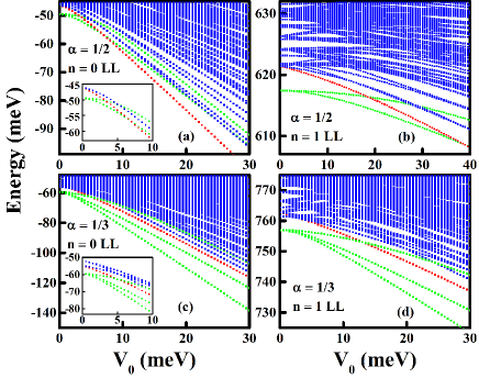
Figure 1: The low-lying four-electron energy levels versus $V_{0}$. The results are for (a) $\alpha=1/2$ and $n=0$ LL,(b) $\alpha=1/2$ and $n=1$ LL, (c) $\alpha=1/3$ and $n=0$ LL, (d) $\alpha=1/3$ and $n=1$ LL. The triplet ground state is shown in green and the first excited state which crosses the ground state is shown in red. The other excited states are shown in blue. The insets show the enlarged version of the crossing point.

In the single-electron case the inclusion of a periodic potential splits the LL into $r$ subbands of equal weight Rauh , if $\alpha=v/r$. In that case, for $\alpha=1/2$ there is no bandgap between the two subbands. Hence the appearance of gaps for the ground and excited states for $\alpha=1/2$ is a direct consequence of the Coulomb interaction Apalkov_14 . The most striking feature in Fig. 1 a,b for $\alpha=1/2$ is the crossing of the excited level with both ground states and change of the ground state at $V_{0}\approx 7$ meV for $n=0$ LL and at $V_{0}\approx 40$ meV for $n=1$ LL. The difference in the value of $V_{0}$ where the ground state changes between the $n=0$ and $n=1$ LL is a direct consequence of the robustness of the FQHE state for $n=1$ LL compared to that of $n=0$ LL, which can be clearly seen also by the magnitude of the gaps for both cases above and was found earlier in graphene mono_FQHE . These crossings and change of the ground state can be characterized as the the crossing of the levels with different CM momentum and also with different relative momentum where the relative momentum is a conserved quantity (see below). In Fig. 1 c,d and for $\alpha=1/3$ we observe similar crossing between the levels and closing of the FQHE gap although there is no ground state change in this case. This is related to the fact that we consider the system with filling factor $\nu=1/3$. For $\alpha=1/3$ this corresponds to the ground state of the system, which will be separated from the excited states by the inclusion of the periodic potential even for non-interacting electrons due to the Hofstadter gap. Even though the inclusion of interaction adds additional gaps to the energy spectra, as can be seen for the excited states in Fig. 1 c,d, the Hofstadter gaps are considerably larger and an increase of $V_{0}$ will not result in a change of the ground state. When $\alpha=1/2$ the filling factor $\nu=1/3$ does not correspond to a special point because as was shown earlier Apalkov_14 , although for $\alpha=1/2$ there are no gaps for non-interacting electrons, interaction opens the gaps and the highest gap is observed for $\nu=1/2$, which corresponds to the crossing points of two subbands in the non-interacting case. Hence, this point results in the change of the ground state for $\alpha=1/2$, closure of the FQHE gap and, afterwards, reappearance of the gap due to the periodic potential.

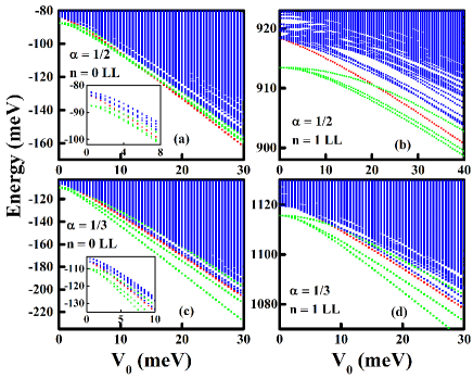
Figure 2: Same as in Fig. 1 but for $N_{e}=6$.

In Fig. 2 the dependence of low-lying energy levels on $V_{0}$ is shown for $N_{e}=6$ and $\alpha=1/2$ and $\alpha=1/3$. The FQHE gap for $n=0$ and $n=1$ LL and $V_{0}=0$ is $\sim$4.02 meV and $\sim$4.85 meV respectively for $\alpha=1/2$, $\sim$4.54 meV and $\sim$5.52 meV for $\alpha=1/3$ respectively. Similar to the case of $N_{e}=4$ and $\alpha=1/2$ we observe the change of the ground state at $V_{0}\approx 16.5$ meV for $n=0$ LL and $V_{0}\approx 91$ meV for $n=1$ LL (not shown in Fig. 2 b). For $\alpha=1/3$ we again observe a crossing between the highest ground state and the excited state, but do not observe any ground state change. The only difference between $N_{e}=6$ and $N_{e}=4$ is the observation of complete lifting of the degeneracy of ground state with the inclusion of the periodic potential, and is related to the fact that for $N_{e}=6$ the relative momentum is a conserved quantity for all cases considered. It should be noted that although the value of $V_{0}$ at which the ground state changes for $\alpha=1/2$ vary considerably with the number of electrons [Fig. 1 (a,b) and Fig. 2 (a,b)], the value of $V_{0}$ at which the closure of the FQHE gap appears is almost the same for both systems.

Just as for $V_{0}=0$, we can define the relative magnetic translations $T^{\mathrm{R}}_{i}(N_{e}\mathbf{a}_{p})=T_{i}(N_{e}\mathbf{a}_{p})T^{\mathrm{CM}}(\mathbf{a}_{p})$, which generally does not commute with the Coulomb interaction term $V_{ij}$ and hence with the Hamiltonian (2), unless $\beta_{1}N_{e}/M_{x}$ and $\beta_{2}N_{e}/M_{y}$ are integers and, in that case, the vector $N_{e}\mathbf{a}_{p}$ is a magnetic translation lattice vector. These conditions are satisfied for all cases considered here, except for $N_{e}=4$ and $\alpha=1/2$. When these conditions are satisfied the absolute values of the relative momentum and the CM momentum eigenvalues are equal and the state can be characterized both by the CM and the relative momentum eigenstates. As is well known haldane_85 ; FQHE_book , without the periodic potential the triply degenerate ground state is characterized by zero relative momentum. Hence for the cases when the conditions above are satisfied and the relative momentum is a conserved quantity, we can state that the three gound states (depicted in green in all figures) correspond to both the relative and the CM momentum equal to zero for all $V_{0}$ and the crossing observed in the figures for the ground states result in the change of the value of relative momentum eigenstate of the ground state.

In conclusion, we have performed the magnetic translation analysis to study the effect of a periodic potential on the FQHE in graphene for filling factor $\nu=1/3$. For $\alpha=1/2$ and $\alpha=1/3$, increasing the periodic potential strength $V_{0}$ results in a closure of the FQHE gap and the appearance of gaps due to the periodic potential. We also find that for $\alpha=1/2$ this results in a change of the ground state and consequently in the change of the ground state momentum. For $\alpha=1/3$, despite the observation of the crossing between the low-lying energy levels, the ground state does not change with an increase of $V_{0}$ and is always characterized by zero momentum. The difference between these two $\alpha$ s is a result of the origin of the gaps for the energy levels. For $\alpha=1/2$ the emergent gaps are due to the electron-electron interaction only, whereas for $\alpha=1/3$ these are both due to the non-interacting Hofstadter butterfly pattern and the electron-electron interaction.

The work has been supported by the Canada Research Chairs Program of the Government of Canada.

References

- (1) Electronic address: Tapash.Chakraborty@umanitoba.ca
- (2) D. Langbein, Phys. Rev. 180, 633 (1969); D. Hofstadter, Phys. Rev. B 14, 2239 (1976).
- (3) M.C. Geisler, J.H. Smet, V. Umansky, K.von Klitzing, B. Naundorf, R. Ketzmerick, and H. Schweizer, Phys. Rev. Lett. 92, 256801 (2004); Physica E 25, 227 (2004); C. Albrecht, J.H. Smet, K. von Klitzing, D. Weiss, V.Umansky, and H. Schweitzer, Phys. Rev. Lett. 86, 147 (2001); Physica E 20, 143 (2003). T. Schlösser, K. Ensslin, J.P. Kotthaus, and M. Holland, Europhys. Lett. 33, 683 (1996); Semicond. Sci. Technol. 11, 1582 (1996).
- (4) C.R. Dean, L. Wang, P. Maher, C. Forsythe, F. Ghahari, Y. Gao, J. Katoch, M. Ishigami, P. Moon, M. Koshino, T. Taniguchi, K.Watanabe, K.L. Shepard, J.Hone, and P. Kim, Nature 497, 598 (2013).
- (5) B. Hunt, J.D. Sanchez-Yamagishi, A.F. Young, M. Yankowitz, B.J. LeRoy, K. Watanabe, T. Taniguchi, P. Moon, M. Koshino, P. Jarillo-Herrero, and R.C. Ashoori, Science 340, 1427 (2013).
- (6) L.A. Ponomarenko, R.V. Gorbachev, G.L. Yu, D.C. Elias, R. Jalil, A.A. Patel, A. Mishchenko, A.S. Mayorov, C.R. Woods, J.R. Wallbank, M. Mucha-Kruczynski, B.A. Piot, M. Potemski, I.V. Grigorieva, K.S. Novoselov, F. Guinea, V.I. Falko and A.K. Geim, Nature 497, 594 (2013).
- (7) D.S.L. Abergel, V. Apalkov, J. Berashevich, K. Ziegler, and T. Chakraborty, Adv. Phys. 59, 261 (2010).
- (8) H. Aoki and M.S. Dresselhaus (Eds.), Physics of Graphene (Springer, New York 2014).
- (9) V.M. Apalkov and T. Chakraborty, Phys. Rev. Lett. 112, 176401 (2014).
- (10) A. Kol and N. Read, Phys. Rev. B 48, 8890 (1993).
- (11) D. Pfannkuche and A.H. MacDonald, Phys. Rev. B 56, R7100 (1997); H. Doh and S.H. Salk, Phys. Rev. B 57, 1312 (1998).
- (12) V.M. Apalkov and T. Chakraborty, Phys. Rev. Lett. 97, 126801 (2006).
- (13) V.M. Apalkov and T. Chakraborty, Phys. Rev. Lett. 105, 036801 (2010); Phys. Rev. Lett. 107, 186803 (2011).
- (14) T. Chakraborty and V. Apalkov, in graphene_book Ch. 8; T. Chakraborty and V.M. Apalkov, Solid State Commun. 175, 123 (2013).
- (15) V. Apalkov and T. Chakraborty, Solid State Commun. 177, 128 (2014); D.S.L. Abergel and T. Chakraborty, Phys. Rev. Lett. 102, 056807 (2009); D. Abergel, V. Apalkov, and T. Chakraborty, Phys. Rev. B 78, 193405 (2008); D. Abergel, P. Pietiläinen, and T. Chakraborty, Phys. Rev.B 80, 081408 (2009); V. Apalkov and T. Chakraborty, Phys. Rev. B 86, 035401 (2012).
- (16) T. Chakraborty and P. Pietiläinen, The Quantum Hall Effects (Springer, New York 1995); T. Chakraborty, and P. Pietiläinen, The Fractional Quantum Hall Effect (Springer, New York 1988).
- (17) X. Du, I. Skachko, F. Duerr, A. Luican, and E.Y. Andrei, Nature 462. 192 (2009); D.A. Abanin, I. Skachko, X. Du, E.Y. Andrei, and L.S. Levitov, Phys. Rev. B 81, 115410 (2010); K.I. Bolotin, F. Ghahari, M.D. Shulman, H.L. Störmer, and P. Kim, Nature 462, 196 (2009); F. Ghahari, Y. Zhao, P. Cadden-Zimansky, K. Bolotin, and P. Kim, Phys. Rev. Lett. 106, 046801 (2011).
- (18) G.L. Yu, R.V. Gorbachev, J.S. Tu, A.V. Kretinin, Y. Cao, R. Jalil, F. Withers, L.A. Ponomarenko, B.A. Piot, M. Potemski, D.C. Elias, X. Chen, K. Watanabe, T. Taniguchi, I.V. Grigorieva, K.S. Novoselov, V.I. Falko, A.K. Geim, and A. Mishchenko, Nat. Phys. 10, 525 (2014).
- (19) J. Zak, Phys. Rev. 133, A1602 (1964); E. Brown, Phys. Rev. 133, A1038 (1964)
- (20) F.D.M. Haldane, Phys. Rev. Lett. 55, 2095 (1985).
- (21) The periodic rectangular geomery was extensively used earlier in the study of the FQHE in various situations. For example, see T. Chakraborty, Surf. Sci. 229, 16 (1990); Adv. Phys. 49, 959 (2000); T. Chakraborty and P. Pietiläinen, Phys. Rev. Lett. 76, 4018 (1996); T. Chakraborty and P. Pietiläinen, Phys. Rev. Lett. 83, 5559 (1999); T. Chakraborty and P. Pietiläinen, Phys. Rev. B 39, 7971 (1989); V.M. Apalkov, T. Chakraborty, P. Pietiläinen, and K. Niemelä, Phys. Rev. Lett. 86, 1311 (2001); T. Chakraborty, P. Pietiläinen, and F.C. Zhang, Phys. Rev. Lett. 57, 130 (1986); T. Chakraborty and F.C. Zhang, Phys. Rev. B 29, 7032 (R) (1984); F.C. Zhang and T. Chakraborty, Phys. Rev. B 30, 7320 (R) (1984).
- (22) A. Rauh, G.H. Wannier, and G. Obermair, Phys. Stat. Sol. (b) 63, 215 (1974).