Method for High Accuracy Multiplicity Correlation Measurements

Abstract

Multiplicity correlation measurements provide insight into the dynamics of high energy collisions. Models describing these collisions need these correlation measurements to tune the strengths of the underlying QCD processes which influence all observables. Detectors, however, often possess limited coverage or reduced efficiency that influence correlation measurements in obscure ways. In this paper, the effects of non-uniform detection acceptance and efficiency on the measurement of multiplicity correlations between two distinct detector regions (termed forward-backward correlations) are derived. An analysis method with such effects built-in is developed and subsequently verified using different event generators. The resulting method accounts for acceptance and efficiency in a model independent manner with high accuracy thereby shedding light on the relative contributions of the underlying processes to particle production.

I Introduction

The charged particles produced in high energy particle collisions are the result of hard and soft interactions. The hard processes are well described by perturbative Quantum Chromodynamics while the soft processes, which occur at low momentum and are the bulk of the interactions, are non-perturbative and, therefore, difficult to describe. This necessitates the use of effective models to characterize these processes. The models must be verified by (and possibly tuned to) experimental results. Therefore, characterization of the properties of the distributions of the produced particles is essential for understanding the soft processes involved in the collisions which are also important for understanding the hard processes as they affect the underlying event. In this paper we focus on the phenomenon called forward-backward particle multiplicity correlations (or forward-backward correlations for short) Sjostrand:1987su to shed light on these soft processes.

Forward-backward correlations measure the correlation strength between the number of particles produced in regions located in opposite hemispheres separated by the plane perpendicular to the beam axis intersecting the collision point. The regions are typically equidistant (angularly) from the plane perpendicular to the beam axis and probe the forward and backward rapidities where most of the particle production is expected. This measurement has the advantage that it is mostly influenced by the dynamics of the collision rather than the following hadronization processes Hwa:2007sq.

Models implement the underlying processes in these collisions in different ways. In Pythia, three main processes exist which affect forward-backward correlations Sjostrand:1987su; Wraight:2011ej. The first process comprises hard scatterings which generally produce forward-backward correlations limited to small angular separations. The second process is initial state radiation which is the emittance of gluons at early times during the interaction and generally causes forward-backward correlations with larger angular separations. The third process is multiple parton interactions which is an effective many-body QCD interaction that causes forward-backward correlations with the largest angular separations. Various tunes of Pythia arise with different contributions from these processes to particle production Skands:2009zm. To investigate which tune more accurately describes reality, one needs to either measure forward-backward correlations with large angular separations (where the net effect of the different contributions is most pronounced) or with high accuracy and precision. Large angular separations are often beyond the design of experiments. High accuracy and precision require advanced techniques to ensure minimal detector bias and are investigated here.

While different measures exist for characterizing forward-backward correlations, in this paper we focus only on the Pearson correlation factor, which we denote as $b$. This correlation factor is defined as: rCl b &≡ Cor(N_f,N_b)=Cov(Nf,Nb)Var(Nf) ⋅Var(Nb)
= ⟨NfNb⟩- ⟨Nf⟩⟨Nb⟩(⟨Nf2⟩- ⟨Nf⟩2) ⋅(⟨Nb2⟩- ⟨Nb⟩2) where $N_{f}$ and $N_{b}$ are the number of particles produced in the regions in the forward and backward hemispheres, respectively.

One important property of the Pearson correlation factor is that it is a bound quantity. It can be shown that $-1\leq b\leq 1$ soegaardPhD and does not scale with the multiplicity of the event. This property arises from the denominator of $b$, which is the square root of the product of the forward and backward multiplicity variances.

Figure 1: The figures depict three sets of forward-backward multiplicity pairs with $b=1,0.6,\textrm{and }0$ from left to right. The variances (used in the denominator of $b$) are the same for $n_{F}$ and $n_{B}$ in all three cases. This demonstrates that the correlation information is essentially contained in the covariance.

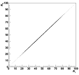
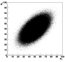
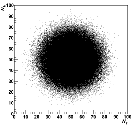
The correlation factor can be interpreted geometrically as how well the set of number pairs describe a line when plotted on a two dimensional figure. This is demonstrated in Fig. 1. The intersection and the slope of the line are irrelevant to the value of $b$ soegaardPhD. This can likewise be demonstrated by the fact that rCl Cor(αX + β, γY + ν) &= Cor(X,Y),   if αγ¿ 0 where $\alpha$, $\beta$, $\gamma$, and $\nu$ are constants. If $\alpha\gamma<0$, the correlation factor switches sign. If the slope in Fig. 1 is negative, the corresponding correlation factor is also negative and the quantities are said to be anti-correlated.

While Eq. (I) shows that only five quantities ($\langle N_{f}\rangle$, $\langle N_{b}\rangle$, $\langle N_{f}N_{b}\rangle$, $\langle N_{f}^{2}\rangle$ and $\langle N_{b}^{2}\rangle$) are necessary to calculate the correlation factor, the measurement is often not trivial to perform for many detector types. Any observable will be altered by the environment surrounding the collision in the experiment. Secondary particle production and partial detector acceptance and inefficiency will influence the measurement. Directly evaluating this influence in a model independent way is challenging for correlation measurements Ravan:2013lwa. This is especially evident when evaluating the variances in the denominator of $b$ when partial acceptance exists. The correlation between the measured and not measured regions requires more sophisticated techniques if the gaps in the acceptance are significant. While the effect of secondary particle production is beyond the scope of this paper (but could be the subject of a subsequent paper), the effect of detector inefficiency and partial detector acceptance is examined. The influence on the measured correlation strength and a means to account for these effects is provided. The method is verified through studies using simulations.

II Measuring the Correlation Factor

While forward-backward correlations can be measured in both collider and fixed target experiments, the investigation here is done for collider experiments. The space surrounding the collision is divided into a forward hemisphere and a backward hemisphere separated by the plane perpendicular to the beam axis intersecting the collision point. The hemisphere where $\theta<\pi/2$ is usually termed forward, and the hemisphere where $\theta>\pi/2$ is usually termed backward, where the reference direction at $\theta=0$ is defined by the experiment.

Forward-backward multiplicity correlations are usually measured between bins of equal width (in $\eta$) spanning the entire azimuth. Correlations between bins where only part of the azimuthal angle is taken into account (twist correlations) can also be measured Wraight:2011ej. While these twist correlations are not directly computed in this paper, they require merely a subset of the information necessary to analyze the full azimuth and, therefore, the techniques presented here could be used with minor modifications to measure twist correlations. The centers of the two bins (in $\eta$) are likewise usually equidistant from $\eta=0$. In this paper we call such a pair of geometrical regions a forward-backward bin.

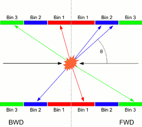
The analysis is carried out by determining the number of particles present in each geometrical region event-by-event. From these particle multiplicities the necessary five quantities are calculated for each event. These five values are then averaged over all events and the correlation factor is calculated. Figure 2 shows an example of how the forward-backward bins are defined.

Figure 2: (Color online) Left: The detector is schematically divided into two halves along the line at $\theta=\pi/2$. Each half then consists of solid angles which span a “small” polar angle and the full azimuthal angle. A forward-backward bin consists of two regions where their centers are equidistant from $\theta=\pi/2$. The regions are often termed forward when $\theta<\pi/2$ and backward when $\theta>\pi/2$. Each forward-backward bin is represented by a different color here. Right: The detector regions have been mapped to a two dimensional figure. The horizontal axis is the pseudorapidity, which is a function of the polar angle, $\theta$. Note that the mapping is not to scale and equal size polar angle bins on the left do not correspond to equal size pseudorapidity bins on the right.

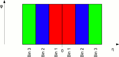
II.1 The Effect of Efficiency

It is common, either by design or due to malfunction, that detectors do not register all particles impinging on them. Full hermeticity does not usually exist either. In both cases, the result is that fewer particles are detected than were actually produced in the collision. This alters the value of an observable. First order observables, like the average number of produced particles, can account for this in a straight-forward manner, since the value scales with the efficiency or acceptance. For higher order observables, the effect of efficiency or acceptance becomes more complex.

To study the effect of efficiency, a statistical approach is taken. In the case of forward-backward correlations, a joint probability distribution for the produced primary particles, $P^{P}(N^{P}_{f},N^{P}_{b})$, contains the physics information one wants to measure. The joint probability distribution is normalized such that rcl ∑_N^P_f=0^∞∑_N^P_b=0^∞P^P(N^P_f,N^P_b) &= 1 A moment generating function can be defined from this whose derivatives evaluated at $t_{f}=0$ and $t_{b}=0$ produce all of the desired moments. rCl mgf^P(t_f,t_b) &≡ ∑_N^P_f=0^∞∑_N^P_b=0^∞P^P(N^P_f,N^P_b) e^N^P_f t_f + N^P_b t_b From the moment generating function, the cumulant generating function is defined as: rCl cgf^P(t_f,t_b) &≡ ln[mgf^P(t_f,t_b)] where derivatives of $\textrm{cgf}^{P}$ evaluated at $t_{f}=0$ and $t_{b}=0$ produce the quantities desired to compute the correlation factor (and many more cumulants with further derivatives). For the purpose of this paper, the first two cumulants (the mean and the covariance) are important. rCl ∂cgfP∂tr(0,0) &≡ cgf^P_r(0,0) = ⟨N_r ⟩,   where r = f or b
∂2cgfP∂tr1∂tr2(0,0) ≡ cgf^P_r_1 r_2(0,0) = Cov(N^P_r_1, N^P_r_2),   where r_1,r_2 = f or b In Eq. (II.1), $r$ stands for a “region” that could be forward or backward. In Eq. (II.1), $r_{1}$ and $r_{2}$ stand for “region 1” and “region 2”, respectively, and can independently be forward or backward. In the case where $r_{1}=r_{2}\textrm{ (}=r\textrm{)}$, the covariance becomes the variance, such that rCl Cov(N^P_r, N^P_r) &= Var(N^P_r)

We now consider the case where a uniform detection efficiency exists over the whole forward and backward regions ($\varepsilon_{f}$ and $\varepsilon_{b}$ respectively). Perfect detection efficiency is defined to have a value of 1 while a completely dead region would have a value of 0. The restriction of uniformity is not realistic, but is instructive for an initial investigation where the efficiency will be taken to be the average detection efficiency in the region. Equation (II.1) is then modified as follows to account these efficiencies in the forward and backward regions. rCl ∑_N^P_f=0^∞∑_N^P_b=0^∞P^P(N^P_f,N^P_b) (ε_f+(1-ε_f))^N^P_f (ε_b+(1-ε_b))^N^P_b &= 1

One can now arrive at the moment generating function for the detected particles ($\textrm{mgf}^{D}$). Since one particle is detected with the probability $\varepsilon_{r}$, one applies the term $e^{1\cdot t_{r}}$ to the $\varepsilon_{r}$ terms. Likewise, one applies $e^{0\cdot t_{r}}=1$ to the $(1-\varepsilon_{r})$ terms, since no particle is detected with this probability. The resulting term, $\varepsilon_{r}e^{t_{r}}+(1-\varepsilon_{r})$, is actually the moment generating function for a specific particle to be found in the region with probability $\varepsilon_{r}$, which we term $\textrm{mgf}^{E}(t_{r};\varepsilon_{r})$. The corresponding cumulant generating function is then $\textrm{cgf}^{E}(t_{r};\varepsilon_{r})\equiv\ln\left[\textrm{mgf}^{E}(t_{r};\varepsilon_{r})\right]$. The moment generating function for the distribution of detected particles then becomes: rCl mgf^D(t_f, t_b)