Solution of linear ill-posed problems using overcomplete dictionaries

Marianna Pensky
Department of Mathematics, University of Central Florida
In memory of Laurent Cavalier
Abstract

In the present paper we consider application of overcomplete dictionaries to solution of general ill-posed linear inverse problems. Construction of an adaptive optimal solution for problems of this sort usually relies either on a singular value decomposition (SVD) or representation of the solution via some orthonormal basis. The shortcoming of both approaches lies in the fact that, in many situations, neither the eigenbasis of the linear operator nor a standard orthonormal basis constitutes an appropriate collection of functions for sparse representation of the unknown function.

In the context of regression problems, there have been an enormous amount of effort to recover an unknown function using an overcomplete dictionary. One of the most popular methods, Lasso and its versions, is based on minimizing the empirical likelihood and requires stringent assumptions on the dictionary, the, so called, compatibility conditions. While these conditions may be satisfied for the original dictionary functions, they usually do not hold for their images due to contraction imposed by the linear operator.

In what follows, we bypass this difficulty by a novel approach which is based on inverting each of the dictionary functions and matching the resulting expansion to the true function, thus, avoiding unrealistic assumptions on the dictionary and using Lasso in a predictive setting. We examine both the white noise and the observational model formulations and also discuss how exact inverse images of the dictionary functions can be replaced by their approximate counterparts. Furthermore, we show how the suggested methodology can be extended to the problem of estimation of a mixing density in a continuous mixture. For all the situations listed above, we provide the oracle inequalities for the risk in a finite sample setting.

We compare the performance of the suggested methodology with the estimators based on the SVD and the orthonormal basis decomposition as well as with the wavelet-vaguelette estimator. Simulation studies confirm good computational properties of the Lasso-based technique.

Keywords and phrases: Linear inverse problem; Lasso; adaptive estimation; oracle inequality

AMS (2000) Subject Classification: Primary: 62G05. Secondary: 62C10

1 Introduction

In this paper, we consider solution of a general ill-posed linear inverse problem Qf=q𝑄𝑓𝑞Qf=q where Q𝑄Q is a bounded linear operator that does not have a bounded inverse and the right-hand side q𝑞q is measured with error. Problems of this kind appear in many areas of application such as astronomy (blurred images), econometrics (instrumental variables), medical imaging (tomography, dynamic contrast enhanced CT and MRI), finance (model calibration of volatility) and many others.

In particular, we consider equation

y=q+ϵη,q=Qf,formulae-sequence𝑦𝑞italic-ϵ𝜂𝑞𝑄𝑓y=q+\sqrt{\epsilon}\eta,\quad q=Qf, (1.1)

where η(t)𝜂𝑡\eta(t) is the Gaussian process representing the noise, ϵitalic-ϵ\sqrt{\epsilon} is the noise level and Q:12:𝑄subscript1subscript2Q:{\cal H}_{1}\to{\cal H}_{2} is a bounded linear operator which does not have a bounded inverse, so problem (1.1) is indeed ill-posed. Here, 1subscript1{\cal H}_{1} and 2subscript2{\cal H}_{2} are Hilbert spaces. We assume that observations are taken as functionals of y𝑦y

y,g2=Qf,g2+ϵη(g),g2,formulae-sequencesubscript𝑦𝑔subscript2subscript𝑄𝑓𝑔subscript2italic-ϵ𝜂𝑔𝑔subscript2\langle y,g\rangle_{{\cal H}_{2}}=\langle Qf,g\rangle_{{\cal H}_{2}}+\sqrt{\epsilon}\,\eta(g),\ \ g\in{\cal H}_{2}, (1.2)

where, for any g2𝑔subscript2g\in{\cal H}_{2}, η(g)𝜂𝑔\eta(g) is a Gaussian random variable with zero mean and variance g22superscriptsubscriptnorm𝑔22\|g\|_{2}^{2} such that 𝔼[η(g1)η(g2)]=g1,g22𝔼delimited-[]𝜂subscript𝑔1𝜂subscript𝑔2subscriptsubscript𝑔1subscript𝑔2subscript2{\mathbb{E}}[\eta(g_{1})\eta(g_{2})]=\langle g_{1},g_{2}\rangle_{{\cal H}_{2}}. Formulation above refers to the scenario where one cannot measure function y(t)𝑦𝑡y(t) everywhere: only functionals of y𝑦y are available. Such functionals, for example, may be coefficients of y𝑦y in some orthonormal basis (e.g., Fourier, wavelet, eigenbasis of Q𝑄Q). The situation where one observes values of function y𝑦y at some points is studied in depth in Section 6.

In order to understand formulation above, consider a common situation where operator Q𝑄Q is of the form

(Qf)(x)=abg(x,t)f(t)𝑑t,x(c,d).formulae-sequence𝑄𝑓𝑥superscriptsubscript𝑎𝑏𝑔𝑥𝑡𝑓𝑡differential-d𝑡𝑥𝑐𝑑(Qf)(x)=\int_{a}^{b}g(x,t)f(t)dt,\quad x\in(c,d). (1.3)

and f(t)𝑓𝑡f(t), g(x,t)𝑔𝑥𝑡g(x,t), q(x)𝑞𝑥q(x) and y(x)𝑦𝑥y(x), t(a,b)𝑡𝑎𝑏t\in(a,b), x(c,d)𝑥𝑐𝑑x\in(c,d), are square integrable functions. In this case, Q:12:𝑄subscript1subscript2Q:{\cal H}_{1}\to{\cal H}_{2} where 1=L2(a,b)subscript1superscript𝐿2𝑎𝑏{\cal H}_{1}=L^{2}(a,b) and 2=L2(c,d)subscript2superscript𝐿2𝑐𝑑{\cal H}_{2}=L^{2}(c,d), the spaces of square integrable functions with the scalar products

f1,f21=abf1(t)f2(t)𝑑t,q1,q21=cdq1(x)q2(x)𝑑x.formulae-sequencesubscriptsubscript𝑓1subscript𝑓2subscript1superscriptsubscript𝑎𝑏subscript𝑓1𝑡subscript𝑓2𝑡differential-d𝑡subscriptsubscript𝑞1subscript𝑞2subscript1superscriptsubscript𝑐𝑑subscript𝑞1𝑥subscript𝑞2𝑥differential-d𝑥\langle f_{1},f_{2}\rangle_{{\cal H}_{1}}=\int_{a}^{b}f_{1}(t)f_{2}(t)dt,\quad\langle q_{1},q_{2}\rangle_{{\cal H}_{1}}=\int_{c}^{d}q_{1}(x)q_{2}(x)dx.

Formula (1.2) refers to the fact that function y(x)=(Qf)(x)+ϵη(x)𝑦𝑥𝑄𝑓𝑥italic-ϵ𝜂𝑥y(x)=(Qf)(x)+\sqrt{\epsilon}\eta(x) cannot be measured for all points x𝑥x: one can only observe linear functionals

y,ψ2=cdy(x)ψ(x)𝑑x=cdq(x)ψ(x)𝑑x+ϵη(ψ),subscript𝑦𝜓subscript2superscriptsubscript𝑐𝑑𝑦𝑥𝜓𝑥differential-d𝑥superscriptsubscript𝑐𝑑𝑞𝑥𝜓𝑥differential-d𝑥italic-ϵ𝜂𝜓\langle y,\psi\rangle_{{\cal H}_{2}}=\int_{c}^{d}y(x)\psi(x)dx=\int_{c}^{d}q(x)\psi(x)dx+\sqrt{\epsilon}\,\eta(\psi),

where η(ψ)N(0,ψ22)similar-to𝜂𝜓𝑁0superscriptsubscriptnorm𝜓22\eta(\psi)\sim N\left(0,\|\psi\|_{2}^{2}\right).

Solutions of statistical inverse problem (1.1) usually rely on reduction of the problem to the sequence model by carrying out the singular value decomposition (SVD) (see, e.g., [8], [9], [10], [17] and [24]), or its relaxed version, the wavelet-vaguelette decomposition proposed by Donoho [15] and further studies by Abramovich and Silverman [2]. Another general approach is Galerkin method with subsequent model selection (see, e.g., [11], [16] and [23]).

The advantage of the methodologies listed above is that they are asymptotically optimal in a minimax sense and, hence, deliver the best possible rates in the “worst case scenario” setting. The function of interest is usually represented via an orthonormal basis which is motivated by the form of the operator Q𝑄Q. However, in spite of being minimax optimal in many contexts, these approaches have two drawbacks. The first one is that, in many situations, these techniques may not be applicable. Indeed, for majority of linear operators, the SVD decomposition is unknown and, hence, cannot be applied. Wavelet-vaguelette decomposition relies on relatively stringent conditions that are satisfied only for specific operators, mainly, of convolution type. In addition, wavelet-based methods are advantageous when one recovers a one-dimensional function defined on a finite interval but do not perform as well for a function of several variables or with an infinite domain. Another shortcoming is that the orthonormal dictionary may not be ”rich enough”. If the unknown function does not have a relatively compact and accurate representation in the chosen basis, the accuracy of the resulting estimator will be poor even though the inverse image of f𝑓f has a moderate norm. In Section 3 we provide detailed explanations how application of overcomplete dictionaries can improve precision of the solutions of ill-posed linear inverse problems.

In the last decade, a great deal of effort was spent on recovery of an unknown function f𝑓f in regression setting from its noisy observations using overcomplete dictionaries. In particular, if the dictionary is large enough and f𝑓f has a sparse representation in this dictionary, then f𝑓f can be recovered with a much better precision than, for example, when it is expanded over an orthonormal basis. The methodology is based on the idea that the error of an estimator of f𝑓f is approximately proportional to the number of dictionary functions that are used for representing f𝑓f, therefore, expanding a function of interest over fewer dictionary elements decreases the estimation error. In order to represent a variety of functions efficiently, one would need to consider a dictionary of much larger size than the number of available observations, the, so called, overcomplete dictionary, and also to develop tools for choosing correct elements of the dictionary that deliver efficient representation of f𝑓f.

A variety of techniques have been developed for solution of those problems such as likelihood penalization methods and greedy algorithms. The most popular of those methods (due to its computational convenience), Lasso and its versions, have been used for solution of a number of theoretical and applied statistical problems (see, e.g., [3], [6], [14], [27], [36], and also [5] and references therein). However, application of Lasso is based on minimizing the empirical likelihood and, unfortunately, requires stringent assumptions on the dictionary {φk}j=1psuperscriptsubscriptsubscript𝜑𝑘𝑗1𝑝\left\{\varphi_{k}\right\}_{j=1}^{p}, the, so called, compatibility conditions. In regression set up, as long as compatibility conditions hold, one can identify the dictionary elements which represent the function of interest best of all at a ”price” which is proportional to ϵlogpitalic-ϵ𝑝\sqrt{\epsilon\,\log p} where p𝑝p is the dictionary size. Regrettably, while compatibility conditions may be satisfied for the functions φjsubscript𝜑𝑗\varphi_{j} in the original dictionary, they usually do not hold for their images Qφj𝑄subscript𝜑𝑗Q\varphi_{j} due to contraction imposed by the operator Q𝑄Q.

In order to illustrate this issue, expand f𝑓f over the dictionary as f𝜽=j=1pθjφjsubscript𝑓𝜽superscriptsubscript𝑗1𝑝subscript𝜃𝑗subscript𝜑𝑗f_{{\mbox{$\theta$}}}=\sum_{j=1}^{p}\theta_{j}\varphi_{j}. Then, q𝜽=j=1pθjujsubscript𝑞𝜽superscriptsubscript𝑗1𝑝subscript𝜃𝑗subscript𝑢𝑗q_{\mbox{$\theta$}}=\sum_{j=1}^{p}\theta_{j}u_{j} with uj=Qφjsubscript𝑢𝑗𝑄subscript𝜑𝑗u_{j}=Q\varphi_{j}. In a nutshell, in order Lasso can recover vector of coefficients 𝜽𝜽\theta correctly, matrix 𝐀𝐀\mathbf{A} with elements Akj=uk,ujsubscript𝐴𝑘𝑗subscript𝑢𝑘subscript𝑢𝑗A_{kj}=\langle u_{k},u_{j}\rangle should be such that its sub-matrices of a small order have eigenvalues that are uniformly separated from zero and infinity (see, e.g. [3]). The latter usually does not hold for the ill-posed problems where the smallest eigenvalue can decrease polynomially or even exponentially as a function of j𝑗j.

The objective of this paper is to circumvent this difficulty and apply Lasso methodology to solution of linear inverse problem (1.1). For thus purpose, in Section 4, instead of matching the expansion q𝜽subscript𝑞𝜽q_{\mbox{$\theta$}} to data y𝑦y, we invert each of the dictionary functions φjsubscript𝜑𝑗\varphi_{j} and match expansion f𝜽subscript𝑓𝜽f_{{\mbox{$\theta$}}} to the true function f𝑓f. This approach has several advantages. First, it allows to use Lasso in a prediction setting where it requires much milder assumptions. In this setting, Lasso converges to the true solution, although at a slow rate, under practically no assumptions on the dictionary. Second, inverting fully known functions φjsubscript𝜑𝑗\varphi_{j} is an easier task than inverting an unknown function measured with noise. In addition, the norms of the inverted images can be viewed as a “price” of including each of the dictionary functions φjsubscript𝜑𝑗\varphi_{j}. In order to ensure that the estimator f𝜽^subscript𝑓^𝜽f_{\widehat{\mbox{$\theta$}}} attains fast convergence rates, we formulate a compatibility assumption and discuss sufficient conditions that guarantee its validity.

The Lasso methodology developed for equations (1.1) and (1.2) allows a variety of generalizations. First, in Section 6, we extend formulations (1.1) and (1.2) to observational model where only the valuesy(ti)𝑦subscript𝑡𝑖y(t_{i}), i=1,,n𝑖1𝑛i=1,\cdots,n, of y(t)𝑦𝑡y(t) are available. Second, in Section 7, we explain how, with very minor modifications, the Lasso technique can be used for estimation of a mixing density in a continuous mixture. Third, in Section 8, we show that, even if the exact inverse images of the dictionary functions do not exist, one can use their approximations and take advantage of the exact knowledge of the dictionary functions which allows the optimal bias-variance decomposition.

We would like to emphasize that the Lasso methodology for solution of linear inverse problems can be viewed as an extension of both the Galerkin method and the wavelet-vaguelette decomposition. Really, if instead of an overcomplete dictionary, one uses an orthonormal basis, then Lasso methodology just reduces to Galerkin method with model selection carried out by a soft thresholding technique. Moreover, if this orthonormal basis is comprised of wavelet functions and conditions for validity of the wavelet-vaguelette decomposition hold, Lasso penalty just imposes soft thresholding on the wavelet coefficients. In order to compare the Lasso estimator with those techniques, we carried out a numerical study of the the Laplace deconvolution problem considered, as an example, in Section 9.2. In particular, together with the Lasso estimator, we implemented the SVD, the wavelet-vaguelette and the Laguerre basis based estimators. Simulation studies confirm that the Lasso estimator developed in the paper has good precision.

The rest of the paper is organized as follows. After introducing notations (Section 2), Section 3 explains why application of overcomplete dictionaries allows to improve estimation precision in linear ill-posed problems. Section 4 develops the theoretical foundations of the paper by justifying application of Lasso technique to solution of general linear inverse problem (1.1). In particular, it introduces a compatibility assumption which guarantees that the Lasso estimator attains fast convergence rates for any function f𝑓f which has a sparse representation in the dictionary. Section 5, discusses this compatibility assumption and formulates simpler sufficient conditions under which it holds. Sections 6 and 7 clarify how this theory can be applied to the real life observational model and also to estimation of a mixing density on the basis of observations of a continuous mixture. Section 8 demonstrates how exact inverse images of the dictionary functions can be replaced by their approximate counterparts. Section 9 contains examples of applications of Lasso to the models studied in the previous sections. Section 10 presents a simulation study. Section 11 concludes the paper with discussion of the results. Finally, Section 12 contains proofs of the statements formulated in earlier sections.

2 Notations

In the paper, we use the following notations.

  • For any vector 𝐭p𝐭superscript𝑝\mathbf{t}\in{\mathbb{R}}^{p}, denote its 2subscript2\ell_{2}, 1subscript1\ell_{1}, 0subscript0\ell_{0} and subscript\ell_{\infty} norms by, respectively, 𝐭2subscriptnorm𝐭2\|\mathbf{t}\|_{2}, 𝐭1subscriptnorm𝐭1\|\mathbf{t}\|_{1}, 𝐭0subscriptnorm𝐭0\|\mathbf{t}\|_{0} and 𝐭subscriptnorm𝐭\|\mathbf{t}\|_{\infty}. Similarly, for any function f𝑓f, denote by f2subscriptnorm𝑓2\|f\|_{2}, f1subscriptnorm𝑓1\|f\|_{1} and fsubscriptnorm𝑓\|f\|_{\infty} its L2subscript𝐿2L_{2}, L1subscript𝐿1L_{1} and Lsubscript𝐿L_{\infty} norms.

  • For any matrix 𝐀𝐀\mathbf{A}, denote its spectral and Frobenius norms by, respectively, 𝐀norm𝐀\|\mathbf{A}\| and 𝐀2subscriptnorm𝐀2\|\mathbf{A}\|_{2}. Notation 𝐀>0𝐀0\mathbf{A}>0 or 𝐀0𝐀0\mathbf{A}\geq 0 means, respectively, that 𝐀𝐀\mathbf{A} is positive or non-negative definite. Denote determinant of 𝐀𝐀\mathbf{A} by |𝐀|𝐀|\mathbf{A}| and the largest, in absolute value, element of 𝐀𝐀\mathbf{A} by 𝐀subscriptnorm𝐀\|\mathbf{A}\|_{\infty}. Denote the Moore-Penrose inverse of matrix 𝐀𝐀\mathbf{A} by 𝐀+superscript𝐀\mathbf{A}^{+}.

  • Denote 𝒫={1,,p}𝒫1𝑝{\mathcal{P}}=\{1,\cdots,p\}. For any subset of indices J𝒫𝐽𝒫J\subseteq{\mathcal{P}}, subset Jcsuperscript𝐽𝑐J^{c} is its complement in 𝒫𝒫{\mathcal{P}} and |J|𝐽|J| is its cardinality, so that |𝒫|=p𝒫𝑝|{\mathcal{P}}|=p. Let J=Span{φj,jJ}subscript𝐽Spansubscript𝜑𝑗𝑗𝐽{\mathcal{L}}_{J}=\mbox{Span}\left\{\varphi_{j},\ j\in J\right\}.

  • If J𝒫𝐽𝒫J\subset{\mathcal{P}} and 𝐭p𝐭superscript𝑝\mathbf{t}\in{\mathbb{R}}^{p}, then 𝐭J|J|subscript𝐭𝐽superscript𝐽\mathbf{t}_{J}\in{\mathbb{R}}^{|J|} denotes reduction of vector 𝐭𝐭\mathbf{t} to subset of indices J𝐽J.

  • Denote by λmin(m;𝚽)subscript𝜆𝑚𝚽\lambda_{\min}(m;\mbox{$\Phi$}) and λmax(m;𝚽)subscript𝜆𝑚𝚽\lambda_{\max}(m;\mbox{$\Phi$}) the minimum and the maximum restricted eigenvalues of matrix 𝚽𝚽\Phi

    λmin(m;𝚽)=min𝐭0m𝐭p𝐭T𝚽𝐭𝐭22,λmax(m;𝚽)=max𝐭0m𝐭p𝐭T𝚽𝐭𝐭22.formulae-sequencesubscript𝜆𝑚𝚽subscriptsuperscriptsubscriptnorm𝐭0𝑚𝐭superscript𝑝superscript𝐭𝑇𝚽𝐭superscriptsubscriptnorm𝐭22subscript𝜆𝑚𝚽subscriptsuperscriptsubscriptnorm𝐭0𝑚𝐭superscript𝑝superscript𝐭𝑇𝚽𝐭superscriptsubscriptnorm𝐭22\lambda_{\min}(m;\mbox{$\Phi$})=\min_{\stackrel{{\scriptstyle\mathbf{t}\in{\mathbb{R}}^{p}}}{{\|\mathbf{t}\|_{0}\leq m}}}\ \frac{\mathbf{t}^{T}\mbox{$\Phi$}\mathbf{t}}{\|\mathbf{t}\|_{2}^{2}},\quad\lambda_{\max}(m;\mbox{$\Phi$})=\max_{\stackrel{{\scriptstyle\mathbf{t}\in{\mathbb{R}}^{p}}}{{\|\mathbf{t}\|_{0}\leq m}}}\ \frac{\mathbf{t}^{T}\mbox{$\Phi$}\mathbf{t}}{\|\mathbf{t}\|_{2}^{2}}. (2.1)

    Also, denote by ϱ(𝚽)italic-ϱ𝚽\varrho(\mbox{$\Phi$}) the maximum of a non-diagonal element of matrix 𝚽𝚽\Phi:

    ϱ(𝚽)=maxjk|Φjk|.italic-ϱ𝚽subscript𝑗𝑘subscriptΦ𝑗𝑘\varrho(\mbox{$\Phi$})=\max_{j\neq k}|\Phi_{jk}|. (2.2)

    Whenever there is no ambiguity, we drop 𝚽𝚽\Phi in the above notations and write simply λmin(m)subscript𝜆𝑚\lambda_{\min}(m), λmax(m)subscript𝜆𝑚\lambda_{\max}(m) and ϱitalic-ϱ\varrho.

  • ambmasymptotically-equalssubscript𝑎𝑚subscript𝑏𝑚a_{m}\asymp b_{m} means that there exist constants 0<C1<C2<0subscript𝐶1subscript𝐶20<C_{1}<C_{2}<\infty independent of m𝑚m such that C1am<bm<C2amsubscript𝐶1subscript𝑎𝑚subscript𝑏𝑚subscript𝐶2subscript𝑎𝑚C_{1}a_{m}<b_{m}<C_{2}a_{m}.

3 Advantages of overcomplete dictionaries

The purpose of this section is to demonstrate how application of a rich overcomplete dictionary can reduce estimation error in inverse linear ill-posed problems. Indeed, if an overcomplete dictionary allows an efficient representation of f𝑓f, it leads to a smaller estimation error. In order to understand the roots of this phenomenon, consider the situation where operator Q𝑄Q has a singular value decomposition Qek=λkek𝑄subscript𝑒𝑘subscript𝜆𝑘subscript𝑒𝑘Qe_{k}=\lambda_{k}e_{k}, k=1,2,𝑘12k=1,2,\cdots, and function f𝑓f can be represented as f=kckek𝑓subscript𝑘subscript𝑐𝑘subscript𝑒𝑘f=\sum_{k}c_{k}e_{k}. Assume, without loss of generality, that for some μ>0𝜇0\mu>0 and ρ>0𝜌0\rho>0

|ck|C0k(μ+1/2)and|λk|Cλkρ.formulae-sequencesubscript𝑐𝑘subscript𝐶0superscript𝑘𝜇12andsubscript𝜆𝑘subscript𝐶𝜆superscript𝑘𝜌|c_{k}|\leq C_{0}k^{-(\mu+1/2)}\quad\mbox{and}\quad|\lambda_{k}|\geq C_{\lambda}k^{-\rho}. (3.1)

In this case, one can construct the SVD estimator f^SVD=k=1mλk1y,ekeksubscript^𝑓𝑆𝑉𝐷superscriptsubscript𝑘1𝑚superscriptsubscript𝜆𝑘1𝑦subscript𝑒𝑘subscript𝑒𝑘\widehat{f}_{SVD}=\sum_{k=1}^{m}\lambda_{k}^{-1}\langle y,e_{k}\rangle\,e_{k} of f𝑓f with the mean squared error (MSE) of the form

𝔼f^SVDf22=k=m+1ck2+ϵk=1mλk2m2μ+ϵm1+2ρϵ2μ2μ+2ρ+1,𝔼superscriptsubscriptnormsubscript^𝑓𝑆𝑉𝐷𝑓22superscriptsubscript𝑘𝑚1superscriptsubscript𝑐𝑘2italic-ϵsuperscriptsubscript𝑘1𝑚superscriptsubscript𝜆𝑘2asymptotically-equalssuperscript𝑚2𝜇italic-ϵsuperscript𝑚12𝜌asymptotically-equalssuperscriptitalic-ϵ2𝜇2𝜇2𝜌1{\mathbb{E}}\|\widehat{f}_{SVD}-f\|_{2}^{2}=\sum_{k=m+1}^{\infty}c_{k}^{2}+\epsilon\sum_{k=1}^{m}\lambda_{k}^{-2}\asymp m^{-2\mu}+\epsilon m^{1+2\rho}\asymp\epsilon^{\frac{2\mu}{2\mu+2\rho+1}}, (3.2)

where the value of m𝑚m is chosen to minimize the right-hand side of (3.2). The advantage of the SVD is that its error rates hold in the “worst case” minimax estimation scenario where f𝑓f is the hardest to estimate in the chosen class of functions.

On the other hand, consider the “best case” scenario when one has an extensive overcomplete dictionary φlsubscript𝜑𝑙\varphi_{l} with φl=1normsubscript𝜑𝑙1\|\varphi_{l}\|=1, l=1,,p𝑙1𝑝l=1,\cdots,p, and f𝑓f is proportional to one of the dictionary functions, say, φjsubscript𝜑𝑗\varphi_{j}. Expand dictionary functions φlsubscript𝜑𝑙\varphi_{l} in the eigenbasis eksubscript𝑒𝑘e_{k} and find their inverse images ψlsubscript𝜓𝑙\psi_{l} obtaining

φl=k=1clkek,ψl=k=1clkλk1ek.formulae-sequencesubscript𝜑𝑙superscriptsubscript𝑘1subscript𝑐𝑙𝑘subscript𝑒𝑘subscript𝜓𝑙superscriptsubscript𝑘1subscript𝑐𝑙𝑘superscriptsubscript𝜆𝑘1subscript𝑒𝑘\varphi_{l}=\sum_{k=1}^{\infty}c_{lk}e_{k},\quad\psi_{l}=\sum_{k=1}^{\infty}c_{lk}\lambda_{k}^{-1}e_{k}.

If one had an oracle which identifies the function φjsubscript𝜑𝑗\varphi_{j} that is proportional to f𝑓f, then cjk=ck/fsubscript𝑐𝑗𝑘subscript𝑐𝑘norm𝑓c_{jk}=c_{k}/\|f\| and f𝑓f would be estimated by f^or=y,ψjφjsubscript^𝑓𝑜𝑟𝑦subscript𝜓𝑗subscript𝜑𝑗\widehat{f}_{or}=\langle y,\psi_{j}\rangle\varphi_{j} with the error

𝔼f^orf22𝔼superscriptsubscriptnormsubscript^𝑓𝑜𝑟𝑓22\displaystyle{\mathbb{E}}\|\widehat{f}_{or}-f\|_{2}^{2} =\displaystyle= ϵψj22=ϵk=1λk2cjk2=ϵf22k=1λk2ck2.italic-ϵsubscriptsuperscriptnormsubscript𝜓𝑗22italic-ϵsuperscriptsubscript𝑘1superscriptsubscript𝜆𝑘2superscriptsubscript𝑐𝑗𝑘2italic-ϵsuperscriptsubscriptnorm𝑓22superscriptsubscript𝑘1superscriptsubscript𝜆𝑘2superscriptsubscript𝑐𝑘2\displaystyle\epsilon\|\psi_{j}\|^{2}_{2}=\epsilon\,\sum_{k=1}^{\infty}\lambda_{k}^{-2}c_{jk}^{2}=\epsilon\,\|f\|_{2}^{-2}\,\sum_{k=1}^{\infty}\lambda_{k}^{-2}c_{k}^{2}. (3.3)

Moreover, if μ>ρ𝜇𝜌\mu>\rho in (3.1), then the series in the right-hand side of (3.3) is convergent and f^orsubscript^𝑓𝑜𝑟\widehat{f}_{or} has parametric error rate 𝔼f^orf2ϵ.asymptotically-equals𝔼superscriptnormsubscript^𝑓𝑜𝑟𝑓2italic-ϵ{\mathbb{E}}\|\widehat{f}_{or}-f\|^{2}\asymp\epsilon. Otherwise, if μρ𝜇𝜌\mu\leq\rho, one can replace ψjsubscript𝜓𝑗\psi_{j} by

ψj,Mj=k=1Mjcjkeksubscript𝜓𝑗subscript𝑀𝑗superscriptsubscript𝑘1subscript𝑀𝑗subscript𝑐𝑗𝑘subscript𝑒𝑘\psi_{j,M_{j}}=\sum_{k=1}^{M_{j}}c_{jk}e_{k} (3.4)

and estimate f𝑓f by f^or,M=y,ψj,Mjφjsubscript^𝑓𝑜𝑟𝑀𝑦subscript𝜓𝑗subscript𝑀𝑗subscript𝜑𝑗\widehat{f}_{or,M}=\langle y,\psi_{j,M_{j}}\rangle\varphi_{j}. It is easy to calculate that

𝔼f^or,Mjf22𝔼superscriptsubscriptnormsubscript^𝑓𝑜𝑟subscript𝑀𝑗𝑓22\displaystyle{\mathbb{E}}\|\widehat{f}_{or,M_{j}}-f\|_{2}^{2} =\displaystyle= [ϵk=1Mjλk2cjk2+k=Mj+1cjk2]ϵMj2ρ2μ+Mj2μ.asymptotically-equalsdelimited-[]italic-ϵsuperscriptsubscript𝑘1subscript𝑀𝑗superscriptsubscript𝜆𝑘2superscriptsubscript𝑐𝑗𝑘2superscriptsubscript𝑘subscript𝑀𝑗1superscriptsubscript𝑐𝑗𝑘2italic-ϵsuperscriptsubscript𝑀𝑗2𝜌2𝜇superscriptsubscript𝑀𝑗2𝜇\displaystyle\left[\epsilon\,\sum_{k=1}^{M_{j}}\lambda_{k}^{-2}c_{jk}^{2}+\sum_{k=M_{j}+1}^{\infty}c_{jk}^{2}\right]\asymp\epsilon{M_{j}}^{2\rho-2\mu}+{M_{j}}^{-2\mu}. (3.5)

Choosing Mjsubscript𝑀𝑗M_{j} that minimizes the right-hand side of (3.5), obtain

𝔼f^or,Mjf22ϵ2μ2ρ=o(ϵ2μ2μ+2ρ+1)𝔼f^SVDf22,ϵ0,formulae-sequenceasymptotically-equals𝔼superscriptsubscriptnormsubscript^𝑓𝑜𝑟subscript𝑀𝑗𝑓22superscriptitalic-ϵ2𝜇2𝜌𝑜superscriptitalic-ϵ2𝜇2𝜇2𝜌1asymptotically-equals𝔼superscriptsubscriptnormsubscript^𝑓𝑆𝑉𝐷𝑓22italic-ϵ0{\mathbb{E}}\|\widehat{f}_{or,M_{j}}-f\|_{2}^{2}\asymp\epsilon^{\frac{2\mu}{2\rho}}=o\left(\epsilon^{\frac{2\mu}{2\mu+2\rho+1}}\right)\asymp{\mathbb{E}}\|\widehat{f}_{SVD}-f\|_{2}^{2},\quad\epsilon\to 0,

i.e. the error of f^or,Mjsubscript^𝑓𝑜𝑟subscript𝑀𝑗\widehat{f}_{or,M_{j}} is smaller than the error of the SVD estimator. The advantage comes from the fact that, unlike in (3.2), in the right-hand sides of (3.3) and (3.5), the “large” values λk2superscriptsubscript𝜆𝑘2\lambda_{k}^{-2} are multiplied by “small” values cjk2superscriptsubscript𝑐𝑗𝑘2c_{jk}^{2} in the expression for the MSE.

One would argue that the assumption that f𝑓f is proportional to one of the dictionary elements is not very realistic. However, it is very likely that f𝑓f can be represented by a small subset of the dictionary functions φj,jJ,subscript𝜑𝑗𝑗𝐽\varphi_{j},j\in J, of cardinality |J|=s𝐽𝑠|J|=s. Then, f𝑓f can be estimated by

f^or,𝐌=jJy,ψj,Mjφj,𝐌=(M1,,Ms)formulae-sequencesubscript^𝑓𝑜𝑟𝐌subscript𝑗𝐽𝑦subscript𝜓𝑗subscript𝑀𝑗subscript𝜑𝑗𝐌subscript𝑀1subscript𝑀𝑠\widehat{f}_{or,\mathbf{M}}=\sum_{j\in J}\langle y,\psi_{j,M_{j}}\rangle\varphi_{j},\quad\mathbf{M}=(M_{1},\cdots,M_{s})

where ψj,Mjsubscript𝜓𝑗subscript𝑀𝑗\psi_{j,M_{j}} are defined in (3.4) and the values Mjsubscript𝑀𝑗M_{j} are found by minimizing the right-hand side of (3.5). If, for example, the dictionary functions are not “much harder” than f𝑓f, i.e., if there exists a constant Cfsubscript𝐶𝑓C_{f} such that for jJ𝑗𝐽j\in J one has cjk2Cfck2superscriptsubscript𝑐𝑗𝑘2subscript𝐶𝑓superscriptsubscript𝑐𝑘2c_{jk}^{2}\leq C_{f}c_{k}^{2}, then 𝔼f^or,𝐌f2sϵasymptotically-equals𝔼superscriptnormsubscript^𝑓𝑜𝑟𝐌𝑓2𝑠italic-ϵ{\mathbb{E}}\|\widehat{f}_{or,\mathbf{M}}-f\|^{2}\asymp s\epsilon if μ>ρ𝜇𝜌\mu>\rho and 𝔼f^or,𝐌f2sϵ2μ2ρasymptotically-equals𝔼superscriptnormsubscript^𝑓𝑜𝑟𝐌𝑓2𝑠superscriptitalic-ϵ2𝜇2𝜌{\mathbb{E}}\|\widehat{f}_{or,\mathbf{M}}-f\|^{2}\asymp s\epsilon^{\frac{2\mu}{2\rho}} otherwise. Note that there is also a significant difference between choosing the optimal values of m𝑚m in (3.2) and Mjsubscript𝑀𝑗M_{j} in (3.5). Indeed, the coefficients of the dictionary functions cjksubscript𝑐𝑗𝑘c_{jk} are known, while coefficients cksubscript𝑐𝑘c_{k} of f𝑓f are unknown, so the latter problem is a straightforward one while the former one is not.

Since one does not have an oracle which allows to choose the “right” subset of dictionary functions φj,jJsubscript𝜑𝑗𝑗𝐽\varphi_{j},j\in J, Lasso is instrumental for choosing an appropriate subset such that, even if it does not coincide with the “true” subset J𝐽J, it provides an estimator of a similar quality.

4 Lasso solution of a general linear inverse problem

Consider equation (1.1) described above with observations defined in (1.2). Denote by Qsuperscript𝑄Q^{*} the conjugate operator for Q𝑄Q, so that Qf,g2=f,Qg1subscript𝑄𝑓𝑔subscript2subscript𝑓superscript𝑄𝑔subscript1\langle Qf,g\rangle_{{\cal H}_{2}}=\langle f,Q^{*}g\rangle_{{\cal H}_{1}} for any f1𝑓subscript1f\in{\cal H}_{1} and g2𝑔subscript2g\in{\cal H}_{2}. Unless there is an ambiguity, in what follows, we denote the scalar product induced norms in both 1subscript1{\cal H}_{1} and 2subscript2{\cal H}_{2} by 2\|\cdot\|_{2}.

Let {φj,j𝒫}subscript𝜑𝑗𝑗𝒫\left\{\varphi_{j},j\in{\mathcal{P}}\right\} be a dictionary such that φj1=1subscriptnormsubscript𝜑𝑗subscript11\|\varphi_{j}\|_{{\cal H}_{1}}=1. Denote by f𝑓f the true solution of the problem (1.1) and by f𝜽subscript𝑓𝜽f_{\mbox{$\theta$}} the projection of this true solution on the linear span of functions {φj,j𝒫}subscript𝜑𝑗𝑗𝒫\left\{\varphi_{j},j\in{\mathcal{P}}\right\} where, for any 𝐭p𝐭superscript𝑝\mathbf{t}\in{\mathbb{R}}^{p}, we denote

f𝐭=j=1ptjφj.subscript𝑓𝐭superscriptsubscript𝑗1𝑝subscript𝑡𝑗subscript𝜑𝑗f_{\mathbf{t}}=\sum_{j=1}^{p}t_{j}\varphi_{j}. (4.1)

If function f𝑓f were known, we would search for the vector of coefficients 𝜽𝜽\theta of f𝜽subscript𝑓𝜽f_{\mbox{$\theta$}} as a solution of the optimization problem

𝜽=argmin𝐭ff𝐭22,𝜽subscript𝐭superscriptsubscriptnorm𝑓subscript𝑓𝐭22\mbox{$\theta$}=\arg\min_{\mathbf{t}}\|f-f_{\mathbf{t}}\|_{2}^{2},

where f𝐭subscript𝑓𝐭f_{\mathbf{t}} is defined in (4.1). Note that, although f𝑓f is unknown,

ff𝐭22=f22+f𝐭222j=1pf,φj1tjsuperscriptsubscriptnorm𝑓subscript𝑓𝐭22superscriptsubscriptnorm𝑓22superscriptsubscriptnormsubscript𝑓𝐭222superscriptsubscript𝑗1𝑝subscript𝑓subscript𝜑𝑗subscript1subscript𝑡𝑗\|f-f_{\mathbf{t}}\|_{2}^{2}=\|f\|_{2}^{2}+\|f_{\mathbf{t}}\|_{2}^{2}-2\sum_{j=1}^{p}\langle f,\varphi_{j}\rangle_{{\cal H}_{1}}t_{j} (4.2)

is the sum of three components where the first one, f22superscriptsubscriptnorm𝑓22\|f\|_{2}^{2}, is independent of 𝐭𝐭\mathbf{t}, and the second one, f𝐭22superscriptsubscriptnormsubscript𝑓𝐭22\|f_{\mathbf{t}}\|_{2}^{2}, is completely known. In order to estimate the last term in (4.2), we assume that the following condition holds:

(A0)  There exist ψj2subscript𝜓𝑗subscript2\psi_{j}\in{\cal H}_{2} such that Qψj=φjsuperscript𝑄subscript𝜓𝑗subscript𝜑𝑗Q^{*}\psi_{j}=\varphi_{j} and νj=ψj2<subscript𝜈𝑗subscriptnormsubscript𝜓𝑗subscript2\nu_{j}=\|\psi_{j}\|_{{\cal H}_{2}}<\infty.

For example, if operator Q𝑄Q is defined by formula (1.3), then ψjsubscript𝜓𝑗\psi_{j} in Assumption (A0) are solutions of the following equations

(Qψj)(t)=cdg(x,t)ψj(x)𝑑x=φj(t),t(a,b).formulae-sequencesuperscript𝑄subscript𝜓𝑗𝑡superscriptsubscript𝑐𝑑𝑔𝑥𝑡subscript𝜓𝑗𝑥differential-d𝑥subscript𝜑𝑗𝑡𝑡𝑎𝑏(Q^{*}\psi_{j})(t)=\int_{c}^{d}g(x,t)\psi_{j}(x)dx=\varphi_{j}(t),\quad t\in(a,b). (4.3)

Observe that equations resulting from Assumption (A0) have completely known right-hand sides. The values of νjsubscript𝜈𝑗\nu_{j} can be viewed as the “price” of estimating coefficient θjsubscript𝜃𝑗\theta_{j} of f𝜽subscript𝑓𝜽f_{\mbox{$\theta$}}. While, in the regression set up, this “price” is uniform for all coefficients, this is no longer true in the case of ill-posed problems. Under Assumption A0, one can write

βj=f,φj1=f,Qψj1=Qf,ψj2=q,ψj2,subscript𝛽𝑗subscript𝑓subscript𝜑𝑗subscript1subscript𝑓superscript𝑄subscript𝜓𝑗subscript1subscript𝑄𝑓subscript𝜓𝑗subscript2subscript𝑞subscript𝜓𝑗subscript2\beta_{j}=\langle f,\varphi_{j}\rangle_{{\cal H}_{1}}=\langle f,Q^{*}\psi_{j}\rangle_{{\cal H}_{1}}=\langle Qf,\psi_{j}\rangle_{{\cal H}_{2}}=\langle q,\psi_{j}\rangle_{{\cal H}_{2}},

so that

βj=𝔼y,ψj2.subscript𝛽𝑗𝔼subscript𝑦subscript𝜓𝑗subscript2\beta_{j}={\mathbb{E}}\langle y,\psi_{j}\rangle_{{\cal H}_{2}}. (4.4)

For this reason, we can replace βj=f,φj1subscript𝛽𝑗subscript𝑓subscript𝜑𝑗subscript1\beta_{j}=\langle f,\varphi_{j}\rangle_{{\cal H}_{1}} in (4.2) by its estimator

β^j=y,ψj2subscript^𝛽𝑗subscript𝑦subscript𝜓𝑗subscript2\widehat{\beta}_{j}=\langle y,\psi_{j}\rangle_{{\cal H}_{2}} (4.5)

and estimate the vector of coefficients 𝜽𝜽\theta by

𝜽^=argmin𝐭{f𝐭222j=1pβ^jtj+αj=1pνj|tj|}.^𝜽subscript𝐭superscriptsubscriptnormsubscript𝑓𝐭222superscriptsubscript𝑗1𝑝subscript^𝛽𝑗subscript𝑡𝑗𝛼superscriptsubscript𝑗1𝑝subscript𝜈𝑗subscript𝑡𝑗\widehat{\mbox{$\theta$}}=\arg\min_{\mathbf{t}}\left\{\|f_{\mathbf{t}}\|_{2}^{2}-2\sum_{j=1}^{p}\widehat{\beta}_{j}t_{j}+\alpha\sum_{j=1}^{p}\nu_{j}|t_{j}|\right\}. (4.6)

Note that (4.6) is the weighted Lasso problem with the penalty parameter α𝛼\alpha. The coefficients νjsubscript𝜈𝑗\nu_{j} in front of |tj|subscript𝑡𝑗|t_{j}| are motivated by the fact that β^jsubscript^𝛽𝑗\widehat{\beta}_{j} are centered normal variables with the variances νj2=ψj22superscriptsubscript𝜈𝑗2subscriptsuperscriptnormsubscript𝜓𝑗22\nu_{j}^{2}=\|\psi_{j}\|^{2}_{2}.

In order to reduce optimization problem (4.6) to familiar matrix formulation, we introduce matrix 𝚽𝚽\Phi with elements Φjk=φj,φksubscriptΦ𝑗𝑘subscript𝜑𝑗subscript𝜑𝑘\Phi_{jk}=\langle\varphi_{j},\varphi_{k}\rangle and vector 𝜷^^𝜷\widehat{\mbox{$\beta$}} with elements β^jsubscript^𝛽𝑗\widehat{\beta}_{j}. Define matrices 𝐖𝐖\mathbf{W} and 𝚼𝚼\Upsilon by

𝐖T𝐖=𝚽,𝚼=diag(ν1,,νp).formulae-sequencesuperscript𝐖𝑇𝐖𝚽𝚼diagsubscript𝜈1subscript𝜈𝑝\mathbf{W}^{T}\mathbf{W}=\mbox{$\Phi$},\quad\mbox{$\Upsilon$}=\mbox{diag}(\nu_{1},\cdots,\nu_{p}). (4.7)

Then, (4.6) can be re-written as

𝜽^=argmin𝐭{𝐭T𝐖𝐖T𝐭2𝐭T𝜷^+α𝚼𝐭1}.^𝜽subscript𝐭superscript𝐭𝑇superscript𝐖𝐖𝑇𝐭2superscript𝐭𝑇^𝜷𝛼subscriptnorm𝚼𝐭1\widehat{\mbox{$\theta$}}=\arg\min_{\mathbf{t}}\left\{\mathbf{t}^{T}\mathbf{W}\mathbf{W}^{T}\mathbf{t}-2\mathbf{t}^{T}\widehat{\mbox{$\beta$}}+\alpha\|\mbox{$\Upsilon$}\mathbf{t}\|_{1}\right\}. (4.8)

Introducing vector 𝜸𝜸\gamma such that 𝐖T𝜸=𝜷^superscript𝐖𝑇𝜸^𝜷\mathbf{W}^{T}\mbox{$\gamma$}=\widehat{\mbox{$\beta$}} we reduce (4.8) to

𝜽^=argmin𝐭{𝐖𝐭𝜸22+α𝚼𝐭1}with𝜸=(𝐖𝐖T)+𝐖𝜷^.formulae-sequence^𝜽subscript𝐭subscriptsuperscriptnorm𝐖𝐭𝜸22𝛼subscriptnorm𝚼𝐭1with𝜸superscriptsuperscript𝐖𝐖𝑇𝐖^𝜷\widehat{\mbox{$\theta$}}=\arg\min_{\mathbf{t}}\left\{\|\mathbf{W}\mathbf{t}-\mbox{$\gamma$}\|^{2}_{2}+\alpha\|\mbox{$\Upsilon$}\mathbf{t}\|_{1}\right\}\quad\mbox{with}\quad\mbox{$\gamma$}=(\mathbf{W}\mathbf{W}^{T})^{+}\mathbf{W}\widehat{\mbox{$\beta$}}. (4.9)

Here, 𝚼𝐭1subscriptnorm𝚼𝐭1\|\mbox{$\Upsilon$}\mathbf{t}\|_{1} is the weighted Lasso penalty, α𝛼\alpha is the penalty parameter and 𝜸𝜸\gamma is the right-hand side. The choices of parameter α𝛼\alpha are discussed at the end of this section in Remark 1.

Since we are interested in recovering f𝑓f rather that 𝜽𝜽\theta itself, we are using Lasso for solution of the prediction problem where it requires milder conditions on the dictionary. In particular, estimator f𝜽^subscript𝑓^𝜽f_{\widehat{\mbox{$\theta$}}} converges to the true function f𝑓f with no additional assumptions on the dictionary.

Theorem 1

Let Assumption A0 hold. Then, for any τ>0𝜏0\tau>0 and any αα0𝛼subscript𝛼0\alpha\geq\alpha_{0}, with probability at least 12pτ12superscript𝑝𝜏1-2p^{-\tau}, one has

f𝜽^f22inf𝐭[f𝐭f22+4αj=1pνj|tj|]superscriptsubscriptnormsubscript𝑓^𝜽𝑓22subscriptinfimum𝐭delimited-[]superscriptsubscriptnormsubscript𝑓𝐭𝑓224𝛼superscriptsubscript𝑗1𝑝subscript𝜈𝑗subscript𝑡𝑗\|f_{\widehat{\mbox{$\theta$}}}-f\|_{2}^{2}\leq\inf_{\mathbf{t}}\left[\|f_{\mathbf{t}}-f\|_{2}^{2}+4\alpha\sum_{j=1}^{p}\nu_{j}|t_{j}|\right] (4.10)

where

α0=2ϵ(τ+1)logp.subscript𝛼02italic-ϵ𝜏1𝑝\alpha_{0}=\sqrt{2\,\epsilon\,(\tau+1)\log p}. (4.11)

If the dictionary is large enough, so that f𝜽=fsubscript𝑓𝜽𝑓f_{\mbox{$\theta$}}=f where vector 𝜽𝜽\theta has support J𝐽J of size |J|=s𝐽𝑠|J|=s and components of 𝜽𝜽\theta are uniformly bounded, then, with high probability, the error of estimating f𝑓f by f𝜽^subscript𝑓^𝜽f_{\widehat{\mbox{$\theta$}}} is f𝜽^f22ϵlogpjJνjasymptotically-equalssuperscriptsubscriptnormsubscript𝑓^𝜽𝑓22italic-ϵ𝑝subscript𝑗𝐽subscript𝜈𝑗\|f_{\widehat{\mbox{$\theta$}}}-f\|_{2}^{2}\asymp\sqrt{\epsilon\,\log p}\,\sum_{j\in J}\nu_{j}. In the case of regression problem, νj=1subscript𝜈𝑗1\nu_{j}=1, so that convergence rate appears as sϵlogp𝑠italic-ϵ𝑝s\sqrt{\epsilon\,\log p} and is called the slow Lasso rate, in comparison with the fast Lasso rate sϵlogp𝑠italic-ϵ𝑝s\epsilon\,\log p that can be obtained only if the, so-called, compatibility assumption (see, e.g., [5]) is satisfied.

In the case of the ill-posed problem (1.1), in order to achieve fast Lasso rate, we also need to formulate a compatibility assumption. For this purpose, consider a set of p𝑝p-dimensional vectors

𝒥(μ,J)={𝐝p:(𝚼𝐝)Jc1μ(𝚼𝐝)J1},μ>1,formulae-sequence𝒥𝜇𝐽conditional-set𝐝superscript𝑝subscriptnormsubscript𝚼𝐝superscript𝐽𝑐1𝜇subscriptnormsubscript𝚼𝐝𝐽1𝜇1{\mathcal{J}}(\mu,J)=\left\{\mathbf{d}\in{\mathbb{R}}^{p}:\ \|(\mbox{$\Upsilon$}\mathbf{d})_{{J^{c}}}\|_{1}\leq\mu\|(\mbox{$\Upsilon$}\mathbf{d})_{J}\|_{1}\right\},\quad\mu>1, (4.12)

where matrix 𝚼𝚼\Upsilon is defined in (4.7). We assume that the following condition holds:

(A)  Matrices 𝚽𝚽\Phi and 𝚼𝚼\Upsilon are such that

κ2(μ,J)=min{𝐝𝒥(μ,J),𝐝20:𝐝T𝚽𝐝Tr(𝚼J2)(𝚼𝐝)J12}>0.\kappa^{2}(\mu,J)=\min\left\{\mathbf{d}\in{\mathcal{J}}(\mu,J),\,\|\mathbf{d}\|_{2}\neq 0:\quad\frac{\mathbf{d}^{T}\mbox{$\Phi$}\mathbf{d}\cdot\mbox{Tr}(\mbox{$\Upsilon$}_{J}^{2})}{\|(\mbox{$\Upsilon$}\mathbf{d})_{J}\|_{1}^{2}}\right\}>0. (4.13)

Assumption (4.13) is not easy to check in practice. For this reason, in the next section, we provide verifiable sufficient conditions that guarantee that condition A holds with κ2(μ,J)superscript𝜅2𝜇𝐽\kappa^{2}(\mu,J) being uniformly bounded below by a quantity which is separated from zero.

Observe that, in the regression setup, 𝚼𝚼\Upsilon is the identity matrix, and condition A reduces to the compatibility condition for general sets in the Section 6.2.3 of [5]. If one has an orthonormal basis instead of an overcomplete dictionary, then matrix 𝚽𝚽\Phi is an identity matrix and, due to Cauchy inequality, κ2(μ,J)1superscript𝜅2𝜇𝐽1\kappa^{2}(\mu,J)\geq 1 for any μ𝜇\mu and J𝐽J. On the other hand, for an orthonormal basis, the bias f𝐭f2subscriptnormsubscript𝑓𝐭𝑓2\|f_{\mathbf{t}}-f\|_{2} in (4.10) may be large. Under conditions A0 and A , one obtains fast convergence rates for the Lasso estimator.

Theorem 2

Let Assumptions A0 and A hold. For any τ>0𝜏0\tau>0, let α=α0(μ+1)/(μ1)𝛼subscript𝛼0𝜇1𝜇1\alpha=\alpha_{0}(\mu+1)/(\mu-1) where α0subscript𝛼0\alpha_{0} is defined in (4.11) and K0=2subscript𝐾02K_{0}=2. Then, with probability at least 12pτ12superscript𝑝𝜏1-2p^{-\tau}, one has

f𝜽^f22inf𝐭,J𝒫[f𝐭f22+4αjJcνj|tj|+4K0μ2(τ+1)(μ1)2κ2(μ,J)ϵlogpjJνj2].superscriptsubscriptnormsubscript𝑓^𝜽𝑓22subscriptinfimum𝐭𝐽𝒫delimited-[]superscriptsubscriptnormsubscript𝑓𝐭𝑓224𝛼subscript𝑗superscript𝐽𝑐subscript𝜈𝑗subscript𝑡𝑗4subscript𝐾0superscript𝜇2𝜏1superscript𝜇12superscript𝜅2𝜇𝐽italic-ϵ𝑝subscript𝑗𝐽superscriptsubscript𝜈𝑗2\|f_{\widehat{\mbox{$\theta$}}}-f\|_{2}^{2}\leq\inf_{\mathbf{t},J\subseteq{\mathcal{P}}}\left[\|f_{\mathbf{t}}-f\|_{2}^{2}+4\alpha\sum_{j\in{J^{c}}}\nu_{j}|t_{j}|+\frac{4K_{0}\mu^{2}(\tau+1)}{(\mu-1)^{2}\kappa^{2}(\mu,J)}\epsilon\log p\ \sum_{j\in J}\nu_{j}^{2}\right]. (4.14)

Therefore,

f𝜽^f22infJ𝒫{ffJ22+4K0μ2(τ+1)(μ1)2κ2(μ,J)ϵlogpjJνj2},superscriptsubscriptnormsubscript𝑓^𝜽𝑓22subscriptinfimum𝐽𝒫superscriptsubscriptnorm𝑓subscript𝑓subscript𝐽224subscript𝐾0superscript𝜇2𝜏1superscript𝜇12superscript𝜅2𝜇𝐽italic-ϵ𝑝subscript𝑗𝐽superscriptsubscript𝜈𝑗2\|f_{\widehat{\mbox{$\theta$}}}-f\|_{2}^{2}\leq\inf_{J\subseteq{\mathcal{P}}}\left\{\|f-f_{{\mathcal{L}}_{J}}\|_{2}^{2}+\frac{4K_{0}\mu^{2}(\tau+1)}{(\mu-1)^{2}\kappa^{2}(\mu,J)}\epsilon\log p\ \sum_{j\in J}\nu_{j}^{2}\right\}, (4.15)

where fJ=projJfsubscript𝑓subscript𝐽subscriptprojsubscript𝐽𝑓f_{{\mathcal{L}}_{J}}=\mbox{proj}_{{\mathcal{L}}_{J}}f.

Note that inequality (4.15) ensures that, up to a logp𝑝\log p factor, the estimator f𝜽^subscript𝑓^𝜽f_{\widehat{\mbox{$\theta$}}} attains the minimum possible mean squared error for a particular function of interest f𝑓f as long as compatibility factor κ(μ,J)𝜅𝜇𝐽\kappa(\mu,J) stays uniformly bounded below. Indeed, if f𝑓f were known, one would choose J𝒫𝐽𝒫J\subseteq{\mathcal{P}} and estimate f𝑓f by its projection f~~𝑓\tilde{f} on Jsubscript𝐽{\mathcal{L}}_{J}, so that the overall error is bounded below by

𝔼f~f22minJ𝒫{ffJ22+ϵλmin(|J|,𝚽)jJνj2},𝔼superscriptsubscriptnorm~𝑓𝑓22subscript𝐽𝒫superscriptsubscriptnorm𝑓subscript𝑓subscript𝐽22italic-ϵsubscript𝜆𝐽𝚽subscript𝑗𝐽superscriptsubscript𝜈𝑗2{\mathbb{E}}\|\tilde{f}-f\|_{2}^{2}\geq\min_{J\subset{\mathcal{P}}}\ \left\{\|f-f_{{\mathcal{L}}_{J}}\|_{2}^{2}+\frac{\epsilon}{\lambda_{\min}(|J|,\mbox{$\Phi$})}\ \sum_{j\in J}\nu_{j}^{2}\right\}, (4.16)

where λmin()subscript𝜆\lambda_{\min}(\cdot) is defined in (2.1). If κ2(μ,J)superscript𝜅2𝜇𝐽\kappa^{2}(\mu,J) is bounded below by a constant, then the lower bound in (4.16) differs from the upper bound in (4.15) by a logarithmic factor logp𝑝\log p that serves as a price for choosing a subset of dictionary functions.

Remark 1

(The choice of the Lasso penalty parameter) Note that Theorems 1 and 2 provide explicit expressions for the penalty parameters α𝛼\alpha that guarantee the slow and the fast Lasso rates. In practice, however, those parameter values may be too high and one gets more precise estimators using some kind of cross validation. Another options is to set α=α^𝛼^𝛼\alpha=\hat{\alpha} where α^=argminα[𝐖𝜽^(α)𝜸22+2ϵp^]^𝛼subscript𝛼subscriptsuperscriptnorm𝐖^𝜽𝛼𝜸222italic-ϵ^𝑝\hat{\alpha}=\arg\min_{\alpha}\left[\|\mathbf{W}\widehat{\mbox{$\theta$}}(\alpha)-\mbox{$\gamma$}\|^{2}_{2}+2\epsilon\hat{p}\right]. Here, 𝐖𝐖\mathbf{W} and 𝜸𝜸\gamma are defined in (4.7) and (4.9), respectively, and p^=dim(𝐖𝜽^active)^𝑝dim𝐖subscript^𝜽𝑎𝑐𝑡𝑖𝑣𝑒\hat{p}=\mbox{dim}(\mathbf{W}\widehat{\mbox{$\theta$}}_{active}), the dimension of the linear space 𝐖𝜽^active𝐖subscript^𝜽𝑎𝑐𝑡𝑖𝑣𝑒\mathbf{W}\widehat{\mbox{$\theta$}}_{active} where 𝜽^activesubscript^𝜽𝑎𝑐𝑡𝑖𝑣𝑒\widehat{\mbox{$\theta$}}_{active} is the reduction of 𝜽^^𝜽\widehat{\mbox{$\theta$}} to the sub-vector of the active coefficients. Here, p^^𝑝\hat{p} can be viewed as the SURE estimator of the number p(α)𝑝𝛼p(\alpha) of parameters in the model (see [31]).

Remark 2

(The choice of overcomplete dictionary) The choice of an overcomplete dictionary in regression problems is usually motivated by two considerations: the dictionary should be rich enough that the function of interest allows sparse representation and also should satisfy compatibility conditions. In the case of the ill-posed regression problems, one has an additional constraint that Assumption A0 should be satisfied with ψj2<subscriptnormsubscript𝜓𝑗subscript2\|\psi_{j}\|_{{\cal H}_{2}}<\infty. As long as this additional constraint holds, the issues of dictionary selection in the regression and the linear ill-posed problems are similar.

5 Discussion of the compatibility condition

Note that condition (4.13) is guaranteed by combination of two kinds of assumptions. As we have already mentioned, since the “price” of estimating coefficients varies from one dictionary function to the other, one needs to make sure that Lasso selects coefficients with relatively low variances and sets to zero the ones with high variances. This would be useful if the true function f𝑓f does not have those components. For this purpose, we consider the set of subsets J𝒫𝐽𝒫J\subset{\mathcal{P}} such that

𝒢(Cν)={J𝒫:maxjJ,jJcνjνjCν}.𝒢subscript𝐶𝜈conditional-set𝐽𝒫subscriptformulae-sequence𝑗𝐽superscript𝑗superscript𝐽𝑐subscript𝜈𝑗subscript𝜈superscript𝑗subscript𝐶𝜈{\mathcal{G}}(C_{\nu})=\left\{J\in{\mathcal{P}}:\ \max_{j\in J,\,j^{\prime}\in{J^{c}}}\frac{\nu_{j}}{\nu_{j^{\prime}}}\leq C_{\nu}\right\}. (5.1)

We assume that the true function f𝑓f is such that its best approximation can be achieved using J𝒢(Cν)𝐽𝒢subscript𝐶𝜈J\in{\mathcal{G}}(C_{\nu}).

(A1) For some Cν>0subscript𝐶𝜈0C_{\nu}>0 one has

J^=argmin{J𝒫:ffJ22+4K0μ2(τ+1)(μ1)2ϵjJνj2}𝒢(Cν).^𝐽:𝐽𝒫superscriptsubscriptnorm𝑓subscript𝑓subscript𝐽224subscript𝐾0superscript𝜇2𝜏1superscript𝜇12italic-ϵsubscript𝑗𝐽superscriptsubscript𝜈𝑗2𝒢subscript𝐶𝜈\widehat{J}=\arg\min\left\{J\subset{\mathcal{P}}:\ \|f-f_{{\mathcal{L}}_{J}}\|_{2}^{2}+\frac{4K_{0}\mu^{2}(\tau+1)}{(\mu-1)^{2}}\,\epsilon\ \sum_{j\in J}\nu_{j}^{2}\right\}\in{\mathcal{G}}(C_{\nu}). (5.2)

Note that Assumption A1 is natural and is similar to the usual assumptions that f𝑓f is smooth and does not have fast oscillating components. In the context of the ill-posed problems, Assumption A1 means that f𝑓f is not “too hard” to estimate.

The second condition needs to ensure that the dictionary {φj,j𝒫}subscript𝜑𝑗𝑗𝒫\left\{\varphi_{j},\ j\in{\mathcal{P}}\right\} is incoherent. The latter can be warranted by one of the following alternative assumptions introduced in [3]. In what follows, λminsubscript𝜆\lambda_{\min}, λmaxsubscript𝜆\lambda_{\max} and ϱitalic-ϱ\varrho refer to matrix 𝚽𝚽\Phi.

(A2(a))  For some s𝑠s, 1sp/21𝑠𝑝21\leq s\leq p/2, some ms𝑚𝑠m\geq s and some constant C0subscript𝐶0C_{0} one has

λmin(s+m)>C0λmax(m),subscript𝜆𝑠𝑚subscript𝐶0subscript𝜆𝑚\lambda_{\min}(s+m)>C_{0}\lambda_{\max}(m), (5.3)

where λmin(s+m)subscript𝜆𝑠𝑚\lambda_{\min}(s+m) and λmax(m)subscript𝜆𝑚\lambda_{\max}(m) are restricted eigenvalues defined in (2.1).

(A2(b))  For some s𝑠s, 1sp/21𝑠𝑝21\leq s\leq p/2, and some constant C0subscript𝐶0C_{0} one has

ϱ<[s(2C0+1)]1,italic-ϱsuperscriptdelimited-[]𝑠2subscript𝐶011\varrho<[s(2C_{0}+1)]^{-1}, (5.4)

where ϱitalic-ϱ\varrho is defined in (2.2).

If Assumption A1 is valid, then one can replace J𝒫𝐽𝒫J\subset{\mathcal{P}} by J𝒢(Cν)𝐽𝒢subscript𝐶𝜈J\in{\mathcal{G}}(C_{\nu}) in the inequality (4.15). For J𝒢(Cν)𝐽𝒢subscript𝐶𝜈J\in{\mathcal{G}}(C_{\nu}), Assumption A2(a) (or A2(b)) yields a convenient lower bound on the compatibility factor κ(μ,J)𝜅𝜇𝐽\kappa(\mu,J). In particular, small modifications of Lemma 4.1. of [3] leads to the following result:

Lemma 1

(Lemma 4.1 of [3]) Let Assumption A2(a) or A2(b) be valid with C0=μCνsubscript𝐶0𝜇subscript𝐶𝜈C_{0}=\mu C_{\nu}. Then, for any set J𝒢(Cν)𝐽𝒢subscript𝐶𝜈J\in{\mathcal{G}}(C_{\nu}) of cardinality |J|s𝐽𝑠|J|\leq s, Assumption A holds with κ2(μ,J)ϑ(s,m)superscript𝜅2𝜇𝐽italic-ϑ𝑠𝑚\kappa^{2}(\mu,J)\geq\vartheta(s,m) where

ϑ(s,m)={λmin(s+m)(1μCνsλmax(m)mλmin(s+m))2if A2(a) holds1[s(2μCν+1)]1if A2(b) holds.italic-ϑ𝑠𝑚casessubscript𝜆𝑠𝑚superscript1𝜇subscript𝐶𝜈𝑠subscript𝜆𝑚𝑚subscript𝜆𝑠𝑚2if A2(a) holdsmissing-subexpressionmissing-subexpression1superscriptdelimited-[]𝑠2𝜇subscript𝐶𝜈11if A2(b) holds\vartheta(s,m)=\left\{\begin{array}[]{ll}\lambda_{\min}(s+m)\left(1-\frac{\mu C_{\nu}\sqrt{s\lambda_{\max}(m)}}{\sqrt{m\lambda_{\min}(s+m)}}\right)^{2}&\mbox{if {\bf A2(a)} holds}\\ &\\ 1-[s(2\mu C_{\nu}+1)]^{-1}&\mbox{if {\bf A2(b)} holds}.\end{array}\right. (5.5)

Combination of (4.15) and (5.5) ensures that if f𝑓f allows sparse representation in the dictionary {φj,j𝒫}subscript𝜑𝑗𝑗𝒫\left\{\varphi_{j},j\in{\mathcal{P}}\right\}, so that set J^^𝐽\widehat{J} in Assumption A1 has at most s𝑠s components, then Lasso provides an optimal (up to a logarithmic factor) representation of the function f𝑓f.

Corollary 1

Let Assumptions A0, A1 and A2(a) or A2(b) hold with some m𝑚m and C0=μCνsubscript𝐶0𝜇subscript𝐶𝜈C_{0}=\mu C_{\nu}. Let set J^^𝐽\widehat{J} in Assumption A1 have at most s𝑠s components: |J^|s^𝐽𝑠|\widehat{J}|\leq s. Then, for any τ>0𝜏0\tau>0 and α=α0(μ+1)/(μ1)𝛼subscript𝛼0𝜇1𝜇1\alpha=\alpha_{0}(\mu+1)/(\mu-1), with probability at least 12pτ12superscript𝑝𝜏1-2p^{-\tau}, one has

f𝜽^f22infJ𝒫{ffJ2+4K0μ2(τ+1)(μ1)2logpϑ(s,m)ϵjJνj2}.superscriptsubscriptnormsubscript𝑓^𝜽𝑓22subscriptinfimum𝐽𝒫superscriptnorm𝑓subscript𝑓subscript𝐽24subscript𝐾0superscript𝜇2𝜏1superscript𝜇12𝑝italic-ϑ𝑠𝑚italic-ϵsubscript𝑗𝐽superscriptsubscript𝜈𝑗2\|f_{\widehat{\mbox{$\theta$}}}-f\|_{2}^{2}\leq\inf_{J\subseteq{\mathcal{P}}}\left\{\|f-f_{{\mathcal{L}}_{J}}\|^{2}+\frac{4K_{0}\,\mu^{2}(\tau+1)}{(\mu-1)^{2}}\ \frac{\log p}{\vartheta(s,m)}\ \epsilon\ \sum_{j\in J}\nu_{j}^{2}\right\}. (5.6)

Finally, we comment about the choice of m𝑚m in Assumption A2(a). Similarly to regression set up, this choice depends on how fast the the minimal eigenvalues of the order m𝑚m sub-matrices of 𝚽𝚽\Phi are decreasing as functions of m𝑚m (see, e.g., [3]).

Remark 3

(Invertible dictionary matrix) Note that if one imposes a somewhat stronger condition

maxjjj|Φjj|κ0<1subscriptsuperscript𝑗subscript𝑗superscript𝑗subscriptΦ𝑗superscript𝑗subscript𝜅01\max_{j^{\prime}}\sum_{j\neq j^{\prime}}|\Phi_{jj^{\prime}}|\leq\kappa_{0}<1 (5.7)

for some κ0>0subscript𝜅00\kappa_{0}>0, then λmin(𝚽)1κ0κ(μ,J)subscript𝜆𝚽1subscript𝜅0𝜅𝜇𝐽\lambda_{\min}(\mbox{$\Phi$})\geq 1-\kappa_{0}\geq\kappa(\mu,J) and Assumption A holds. This is a “low-dimensional” application of Lasso technique which, however, may be of use in some practical situations.

6 Observational model

Consider a real-life observational model corresponding to equation (1.1)

yi=q(xi)+ξi,i=1,,n,formulae-sequencesubscript𝑦𝑖𝑞subscript𝑥𝑖subscript𝜉𝑖𝑖1𝑛y_{i}=q(x_{i})+\xi_{i},\quad i=1,\cdots,n, (6.1)

where ξisubscript𝜉𝑖\xi_{i} are i.i.d. centered sub-gaussian random variables such that for some σ𝜎\sigma and any t𝑡t

(|ξi|>t)exp(t2/2σ2).subscript𝜉𝑖𝑡superscript𝑡22superscript𝜎2{\mathbb{P}}\left(|\xi_{i}|>t\right)\leq\exp(-t^{2}/2\sigma^{2}). (6.2)

Assume that xi𝒳subscript𝑥𝑖𝒳x_{i}\in{\cal{X}}, i=1,,n𝑖1𝑛i=1,\cdots,n, are fixed non-random points where y(x)𝑦𝑥y(x) in equation (1.1) is measured. To be more specific, we consider the case when 𝒳=[a,b]𝒳𝑎𝑏{\cal{X}}=[a,b] is an interval, a=x0<x1<xn=b𝑎subscript𝑥0subscript𝑥1subscript𝑥𝑛𝑏a=x_{0}<x_{1}<\cdots x_{n}=b and 2=L2[a,b]subscript2superscript𝐿2𝑎𝑏{\cal H}_{2}=L^{2}[a,b], so that

βj=q,ψj2=𝒳q(x)ψj(x)𝑑x.subscript𝛽𝑗subscript𝑞subscript𝜓𝑗subscript2subscript𝒳𝑞𝑥subscript𝜓𝑗𝑥differential-d𝑥\beta_{j}=\langle q,\psi_{j}\rangle_{{\cal H}_{2}}=\int_{{\cal{X}}}q(x)\psi_{j}(x)dx. (6.3)

Denote T=ba𝑇𝑏𝑎T=b-a, Δxi=xixi1Δsubscript𝑥𝑖subscript𝑥𝑖subscript𝑥𝑖1\Delta x_{i}=x_{i}-x_{i-1} and define new values of νjsubscript𝜈𝑗\nu_{j} and β^jsubscript^𝛽𝑗\widehat{\beta}_{j}

β^j=1ni=1nyiψj(xi)Δxi,νj2=T2ni=1nψj2(xi).formulae-sequencesubscript^𝛽𝑗1𝑛superscriptsubscript𝑖1𝑛subscript𝑦𝑖subscript𝜓𝑗subscript𝑥𝑖Δsubscript𝑥𝑖superscriptsubscript𝜈𝑗2superscript𝑇2𝑛superscriptsubscript𝑖1𝑛superscriptsubscript𝜓𝑗2subscript𝑥𝑖\widehat{\beta}_{j}=\frac{1}{n}\ \sum_{i=1}^{n}y_{i}\psi_{j}(x_{i})\Delta x_{i},\quad\nu_{j}^{2}=\frac{T^{2}}{n}\ \sum_{i=1}^{n}\psi_{j}^{2}(x_{i}). (6.4)

We search for 𝜽^^𝜽\widehat{\mbox{$\theta$}} as a solution of optimization problem (4.8) with β^jsubscript^𝛽𝑗\widehat{\beta}_{j} and νjsubscript𝜈𝑗\nu_{j} given by (6.4). We expect that, if |Δxi|Δsubscript𝑥𝑖|\Delta x_{i}| are small and n𝑛n is large enough, one can estimate f𝑓f on the basis of discrete data in (6.1) as well as on the basis of the white noise model (1.1). Denote

=max1jp[1νjmaxx𝒳|d[q(x)ψj(x)]dx|].subscript1𝑗𝑝1subscript𝜈𝑗subscript𝑥𝒳𝑑delimited-[]𝑞𝑥subscript𝜓𝑗𝑥𝑑𝑥\aleph=\max_{1\leq j\leq p}\left[\frac{1}{\nu_{j}}\ \max_{x\in{\cal{X}}}\left|\frac{d[q(x)\psi_{j}(x)]}{dx}\right|\,\right]. (6.5)

Then, the following statement holds.

Theorem 3

Let Assumptions A0 and A hold and τ>0𝜏0\tau>0 be an arbitrary constant. If for some non-negative constant ϑitalic-ϑ\vartheta one has

maxi|Δxi|ϑTnandn𝒩=T424K0σ2(τ+1)logp,formulae-sequencesubscript𝑖Δsubscript𝑥𝑖italic-ϑ𝑇𝑛and𝑛𝒩superscript𝑇4superscript24subscript𝐾0superscript𝜎2𝜏1𝑝\max_{i}|\Delta x_{i}|\leq\vartheta\,\frac{T}{n}\quad\mbox{and}\quad n\geq{\cal N}=\frac{T^{4}\,\aleph^{2}}{4K_{0}\,\sigma^{2}(\tau+1)\log p}, (6.6)

then, for α0=2ϑn1/2σ2(τ+1)logpsubscript𝛼02italic-ϑsuperscript𝑛12𝜎2𝜏1𝑝\alpha_{0}=2\vartheta\,n^{-1/2}\,\sigma\ \sqrt{2(\tau+1)\log p}, α=α0(μ+1)/(μ1)𝛼subscript𝛼0𝜇1𝜇1\alpha=\alpha_{0}(\mu+1)/(\mu-1) and K0=8ϑ2subscript𝐾08superscriptitalic-ϑ2K_{0}=8\vartheta^{2}, with probability at least 1epτ1𝑒superscript𝑝𝜏1-ep^{-\tau}, inequalities (4.14) and (4.15) hold.

Note that the estimator f𝜽^subscript𝑓^𝜽f_{\widehat{\mbox{$\theta$}}} is fully adaptive since α0subscript𝛼0\alpha_{0} is known. The lower bound n𝒩𝑛𝒩n\geq{\cal N} for n𝑛n is motivated by the fact that the rectangular rule approximations of the integrals in (6.3) should be close in value to those integrals. In addition, if functions ψjsubscript𝜓𝑗\psi_{j} and q𝑞q are smooth, so that functions qψj𝑞subscript𝜓𝑗q\psi_{j} have uniformly bounded second derivatives, one can replace the rectangular rule for calculating βjsubscript𝛽𝑗\beta_{j} by the trapezoid rule. In this case, oracle inequalities in Theorem 3 can be obtained with a smaller value of 𝒩𝒩{\cal N}.

7 Lasso recovery of a mixing density from a continuous mixture

In this section we show that, with a small modification, the method used in the previous sections, can be applied to estimation of the mixing density in a continuous mixture. Consider the situation when one observes a random sample Y1,Y2,,Ynsubscript𝑌1subscript𝑌2subscript𝑌𝑛Y_{1},Y_{2},\cdots,Y_{n} of a random variable Y𝑌Y with an unknown probability density function q(y)𝑞𝑦q(y), y𝒴𝑦𝒴y\in{\cal{Y}}, of the form

q(y)=𝒳g(y|x)f(x)𝑑x,y𝒴,formulae-sequence𝑞𝑦subscript𝒳𝑔conditional𝑦𝑥𝑓𝑥differential-d𝑥𝑦𝒴q(y)=\int_{{\cal{X}}}g(y|x)f(x)dx,\quad y\in{\cal{Y}}, (7.1)

where g(y|x)𝑔conditional𝑦𝑥g(y|x) is a known conditional density of Y𝑌Y given X=x𝑋𝑥X=x, x𝒳𝑥𝒳x\in{\cal{X}}, and f(x)𝑓𝑥f(x), x𝒳𝑥𝒳x\in{\cal{X}}, is an unknown mixing density of interest. If g(y|x)=g(yx)𝑔conditional𝑦𝑥𝑔𝑦𝑥g(y|x)=g(y-x), then problem (7.1) reduces to the extensively studied density deconvolution problem (see, e.g., [28] and references therein). In a general set up, problem (7.1) is usually solved by expanding f𝑓f over some orthonormal dictionary and then recovering coefficients of the expansion (see, e.g., [13], [22] and [34]), by the kernel method (see, e.g., [18]) or by maximizing the empirical likelihood (see, e.g., [26]). It is easy to see that when the conditional density g(y|x)𝑔conditional𝑦𝑥g(y|x) is known, the problem of recovering f𝑓f in (7.1) on the basis of observations from q𝑞q can be viewed as a particular case of the linear inverse problem (6.1) with the main difference that one can sample from the pdf q𝑞q instead of having noisy observations of the values of q𝑞q. Hence, one can easily estimate any linear functional of q𝑞q, so that observations are taken in the form (1.2). For this reason, in this set up, one again can benefit from using a large overcomplete dictionary which allows a compact representation of f𝑓f.

Let, as before, {φk}k=1psuperscriptsubscriptsubscript𝜑𝑘𝑘1𝑝\left\{\varphi_{k}\right\}_{k=1}^{p} be a dictionary and function f𝑓f be expanded over this dictionary yielding its approximation (4.1). The goal is to recover the vector of coefficients 𝜽𝜽\theta. By introducing Hilbert spaces 1=L2(𝒳)subscript1superscript𝐿2𝒳{\cal H}_{1}=L^{2}({\cal{X}}) and 2=L2(𝒴)subscript2superscript𝐿2𝒴{\cal H}_{2}=L^{2}({\cal{Y}}) and a linear operator Q:12:𝑄subscript1subscript2Q:{\cal H}_{1}\rightarrow{\cal H}_{2} given by

(Qf)(y)=𝒳g(y|x)f(x)𝑑xwith(Qu)(x)=𝒴g(y|x)u(y)𝑑y,formulae-sequence𝑄𝑓𝑦subscript𝒳𝑔conditional𝑦𝑥𝑓𝑥differential-d𝑥withsuperscript𝑄𝑢𝑥subscript𝒴𝑔conditional𝑦𝑥𝑢𝑦differential-d𝑦(Qf)(y)=\int_{{\cal{X}}}g(y|x)f(x)dx\quad\mbox{with}\quad(Q^{*}u)(x)=\int_{{\cal{Y}}}g(y|x)u(y)dy, (7.2)

one can essentially reduce the problem (7.1) to (1.1).

Note that, despite the fact that the idea of this section seems to be similar to [7], we consider a different problem and apply a completely novel approach. Indeed, although in [7], the authors estimated the unknown pdf by an expansion over an overcomplete dictionary with coefficients subsequently recovered by Lasso, they assumed that observations from the density of interest are available which makes their problem similar to the regression problem. On the contrary, in our case, observations from the density of interest are unavailable which leads to the difficulties that are experienced in the context of the ill-posed linear inverse problems. Really, though expansion (4.1) leads to q=jθjuj𝑞subscript𝑗subscript𝜃𝑗subscript𝑢𝑗q=\sum_{j}\theta_{j}u_{j} with uj=Qφjsubscript𝑢𝑗𝑄subscript𝜑𝑗u_{j}=Q\varphi_{j}, due to contraction imposed by operator Q𝑄Q, the system of functions {uj,j𝒫}subscript𝑢𝑗𝑗𝒫\left\{u_{j},\ j\in{\mathcal{P}}\right\} does not meet compatibility condition even if {φj,j𝒫}subscript𝜑𝑗𝑗𝒫\left\{\varphi_{j},\ j\in{\mathcal{P}}\right\} does. On the other hand, if one starts with an incoherent dictionary {uj,j𝒫}subscript𝑢𝑗𝑗𝒫\left\{u_{j},j\in{\mathcal{P}}\right\}, the system of functions vj=Q1ujsubscript𝑣𝑗superscript𝑄1subscript𝑢𝑗v_{j}=Q^{-1}u_{j} may be totally inappropriate for estimating f𝑓f.

In order to apply methodology of Section 4, we define new values of βjsubscript𝛽𝑗\beta_{j}, β^jsubscript^𝛽𝑗\widehat{\beta}_{j} and νjsubscript𝜈𝑗\nu_{j}

βj=𝔼[ψj(Y1)],β^j=1ni=1nψj(Yi),νj=ψj.formulae-sequencesubscript𝛽𝑗𝔼delimited-[]subscript𝜓𝑗subscript𝑌1formulae-sequencesubscript^𝛽𝑗1𝑛superscriptsubscript𝑖1𝑛subscript𝜓𝑗subscript𝑌𝑖subscript𝜈𝑗subscriptnormsubscript𝜓𝑗\beta_{j}={\mathbb{E}}[\psi_{j}(Y_{1})],\quad\widehat{\beta}_{j}=\frac{1}{n}\ \sum_{i=1}^{n}\psi_{j}(Y_{i}),\quad\nu_{j}=\|\psi_{j}\|_{\infty}. (7.3)

We search for 𝜽^^𝜽\widehat{\mbox{$\theta$}} as a solution of optimization problem (4.6) with β^jsubscript^𝛽𝑗\widehat{\beta}_{j} and νjsubscript𝜈𝑗\nu_{j} given by (7.3). Then, the following statement is true.

Theorem 4

Let Assumptions A0 and A hold. Let β^jsubscript^𝛽𝑗\widehat{\beta}_{j} and νjsubscript𝜈𝑗\nu_{j} be defined in (7.3), τ𝜏\tau be any positive constant and α0=2n1/2(τ+1)logpsubscript𝛼02superscript𝑛12𝜏1𝑝\alpha_{0}=2\,n^{-1/2}\,\sqrt{(\tau+1)\log p}. Denote α=α0(μ+1)/(μ1)𝛼subscript𝛼0𝜇1𝜇1\alpha=\alpha_{0}(\mu+1)/(\mu-1). If n𝒩0=16/9(τ+1)logp𝑛subscript𝒩0169𝜏1𝑝n\geq{\cal N}_{0}=16/9(\tau+1)\log p, then, with probability at least 12pτ12superscript𝑝𝜏1-2p^{-\tau}, one has

f𝜽^f22inf𝐭[f𝐭f2+4αjJcνj|tj|+16μ2(τ+1)(μ1)2κ2(μ,J)logpnjJνj2].superscriptsubscriptnormsubscript𝑓^𝜽𝑓22subscriptinfimum𝐭delimited-[]superscriptnormsubscript𝑓𝐭𝑓24𝛼subscript𝑗superscript𝐽𝑐subscript𝜈𝑗subscript𝑡𝑗16superscript𝜇2𝜏1superscript𝜇12superscript𝜅2𝜇𝐽𝑝𝑛subscript𝑗𝐽superscriptsubscript𝜈𝑗2\|f_{\widehat{\mbox{$\theta$}}}-f\|_{2}^{2}\leq\inf_{\mathbf{t}}\left[\|f_{\mathbf{t}}-f\|^{2}+4\alpha\sum_{j\in{J^{c}}}\nu_{j}|t_{j}|+\frac{16\mu^{2}(\tau+1)}{(\mu-1)^{2}\kappa^{2}(\mu,J)}\,\frac{\log p}{n}\ \sum_{j\in J}\nu_{j}^{2}\right]. (7.4)
Remark 4

(Smaller penalties) Note that νj2=ψj2superscriptsubscript𝜈𝑗2subscriptsuperscriptnormsubscript𝜓𝑗2\nu_{j}^{2}=\|\psi_{j}\|^{2}_{\infty} in (7.3) can be replaced by a smaller value νj2=Var[ψj(Y1)]superscriptsubscript𝜈𝑗2Vardelimited-[]subscript𝜓𝑗subscript𝑌1\nu_{j}^{2}=\mbox{Var}[\psi_{j}(Y_{1})] which leads to a smaller overall error, provided the number of observations n𝑛n is large enough, in particular,

n𝒩1=max1jp[16(τ+1)logpψj29Var[ψj]].𝑛subscript𝒩1subscript1𝑗𝑝16𝜏1𝑝superscriptsubscriptnormsubscript𝜓𝑗29Vardelimited-[]subscript𝜓𝑗n\geq{\cal N}_{1}=\max_{1\leq j\leq p}\ \left[\frac{16\,(\tau+1)\log p\,\|\psi_{j}\|_{\infty}^{2}}{9\,\mbox{Var}[\psi_{j}]}\right].

Note that, though Var[ψj(Y1)]Vardelimited-[]subscript𝜓𝑗subscript𝑌1\mbox{Var}[\psi_{j}(Y_{1})] is unavailable (since f𝑓f is unknown), one can easily construct an upper bound for νj2superscriptsubscript𝜈𝑗2\nu_{j}^{2}

νj2maxx𝒳[𝒴g(y|x)ψj2(y)𝑑y]superscriptsubscript𝜈𝑗2subscript𝑥𝒳subscript𝒴𝑔conditional𝑦𝑥superscriptsubscript𝜓𝑗2𝑦differential-d𝑦\nu_{j}^{2}\leq\max_{x\in{\cal{X}}}\,\left[\int_{{\cal{Y}}}g(y|x)\psi_{j}^{2}(y)dy\right] (7.5)

or estimate Var[ψj(Y1)]Vardelimited-[]subscript𝜓𝑗subscript𝑌1\mbox{Var}[\psi_{j}(Y_{1})] from observations.

Remark 5

(Estimation by a density function) Estimator f𝜽^subscript𝑓^𝜽f_{\widehat{\mbox{$\theta$}}} obtained as a solution of optimization problem (4.6) with β^jsubscript^𝛽𝑗\widehat{\beta}_{j} and νjsubscript𝜈𝑗\nu_{j} given by (7.3) is not necessarily a probability density function since we do not require the dictionary functions to be nonnegative and the weights to be such that f𝜽^subscript𝑓^𝜽f_{\widehat{\mbox{$\theta$}}} integrates to one. This, however, can be easily accomplished in the context of Lasso estimator if one uses dictionary functions that are pdfs themselves and add constraints that the coefficients are nonnegative and sum to one. Note that since we are using the weighted Lasso penalty, those constraints do not allow to get rid of the penalty term altogether though the non-negativity condition should make compatibility assumption (A) weaker. However, pursuing this extension of the Lasso solution is a matter of future investigations.

8 Approximate inverse images of the dictionary functions

Condition A0 requires that each dictionary function φjsubscript𝜑𝑗\varphi_{j} allows an exact inverse image ψjsubscript𝜓𝑗\psi_{j} such that Qψj=φjsuperscript𝑄subscript𝜓𝑗subscript𝜑𝑗Q^{*}\psi_{j}=\varphi_{j} and νj=ψj2<subscript𝜈𝑗subscriptnormsubscript𝜓𝑗2\nu_{j}=\|\psi_{j}\|_{2}<\infty. This may not always be true since functions ψjsubscript𝜓𝑗\psi_{j} may not be easy to construct or they may have infinite norms. In this situation, arguments of Section 3 suggest that exact inverse images ψjsubscript𝜓𝑗\psi_{j} can be replaced by approximate ones ψj,δsubscript𝜓𝑗𝛿\psi_{j,\delta}.

First, let us consider the setting of Section 4 where observations are taken in the form (1.2) and 1subscript1{{\cal H}_{1}} and 2subscript2{{\cal H}_{2}} are spaces of square integrable functions. Let functions φj,δsubscript𝜑𝑗𝛿\varphi_{j,\delta} be such that φj,δφj2δjsubscriptnormsubscript𝜑𝑗𝛿subscript𝜑𝑗2subscript𝛿𝑗\|\varphi_{j,\delta}-\varphi_{j}\|_{2}\leq\delta_{j} and ψj,δsubscript𝜓𝑗𝛿\psi_{j,\delta} is the solution of the equation Qψj,δ=φj,δsuperscript𝑄subscript𝜓𝑗𝛿subscript𝜑𝑗𝛿Q^{*}\psi_{j,\delta}=\varphi_{j,\delta} with νj,δ=ψj,δ2<subscript𝜈𝑗𝛿subscriptnormsubscript𝜓𝑗𝛿2\nu_{j,\delta}=\|\psi_{j,\delta}\|_{2}<\infty. Then, β^j,δ=y,ψj,δsubscript^𝛽𝑗𝛿𝑦subscript𝜓𝑗𝛿\widehat{\beta}_{j,\delta}=\langle y,\psi_{j,\delta}\rangle, so that

β^j,δ=βj+ϵνj,δηj+hj,hj=q,ψj,δψj.formulae-sequencesubscript^𝛽𝑗𝛿subscript𝛽𝑗italic-ϵsubscript𝜈𝑗𝛿subscript𝜂𝑗subscript𝑗subscript𝑗𝑞subscript𝜓𝑗𝛿subscript𝜓𝑗\widehat{\beta}_{j,\delta}=\beta_{j}+\sqrt{\epsilon}\nu_{j,\delta}\eta_{j}+h_{j},\quad h_{j}=\langle q,\psi_{j,\delta}-\psi_{j}\rangle. (8.1)

where ηjsubscript𝜂𝑗\eta_{j} are standard normal variables. Hence, application of Lemma 3 with K=2𝐾2K=\sqrt{2},

Chδ=max1jp|q,ψj,δψj|νj,δ2ϵlogp(τ+1),Cαδ=2(τ+1)(1+Chδ)formulae-sequencesubscript𝐶𝛿subscript1𝑗𝑝𝑞subscript𝜓𝑗𝛿subscript𝜓𝑗subscript𝜈𝑗𝛿2italic-ϵ𝑝𝜏1subscript𝐶𝛼𝛿2𝜏11subscript𝐶𝛿C_{h\delta}=\max_{1\leq j\leq p}\frac{|\langle q,\psi_{j,\delta}-\psi_{j}\rangle|}{\nu_{j,\delta}\,\sqrt{2\,\epsilon\,\log p\,(\tau+1)}},\quad C_{\alpha\delta}=\sqrt{2(\tau+1)}(1+C_{h\delta}) (8.2)

and α0=Cαδϵlogpsubscript𝛼0subscript𝐶𝛼𝛿italic-ϵ𝑝\alpha_{0}=C_{\alpha\delta}\sqrt{\epsilon\log p}, for any τ>0𝜏0\tau>0 and any αα0𝛼subscript𝛼0\alpha\geq\alpha_{0}, with probability at least 12pτ12superscript𝑝𝜏1-2p^{-\tau}, yields (4.10), (4.14) and (4.15) with K0=2(1+Chδ)2subscript𝐾02superscript1subscript𝐶𝛿2K_{0}=2(1+C_{h\delta})^{2}.

The practical question, however, is how can one construct the functions φj,δsubscript𝜑𝑗𝛿\varphi_{j,\delta} and ψj,δsubscript𝜓𝑗𝛿\psi_{j,\delta}. Consider operator QQ:11:𝑄superscript𝑄subscript1subscript1QQ^{*}:{\cal H}_{1}\to{\cal H}_{1} and a small parameter δ𝛿\delta. Construct functions ψj,δ=(QQ+δI)1Qφjsubscript𝜓𝑗𝛿superscript𝑄superscript𝑄𝛿𝐼1𝑄subscript𝜑𝑗\psi_{j,\delta}=(QQ^{*}+\delta I)^{-1}Q\varphi_{j} where I:11:𝐼subscript1subscript1I:{\cal H}_{1}\to{\cal H}_{1} is the identity operator. Then, one can easily check that relation (8.1) holds. The value of δ𝛿\delta can be chosen so to minimize the mean squared error of estimating βjsubscript𝛽𝑗\beta_{j} by β^j,δsubscript^𝛽𝑗𝛿\widehat{\beta}_{j,\delta} given by

𝔼(β^j,δβj)2=ϵνj,δ2+[q,ψj,δψj]2,𝔼superscriptsubscript^𝛽𝑗𝛿subscript𝛽𝑗2italic-ϵsuperscriptsubscript𝜈𝑗𝛿2superscriptdelimited-[]𝑞subscript𝜓𝑗𝛿subscript𝜓𝑗2{\mathbb{E}}(\widehat{\beta}_{j,\delta}-\beta_{j})^{2}=\epsilon\nu_{j,\delta}^{2}+[\langle q,\psi_{j,\delta}-\psi_{j}\rangle]^{2}, (8.3)

Although function q𝑞q in (8.3) is unknown, one can minimize (8.3) with q𝑞q being replaced by an estimator. Whenever observations are available in the form (1.2) or (6.1), one can construct a kernel or a projection estimator q^^𝑞\hat{q} of q𝑞q and replace q𝑞q by q^^𝑞\hat{q} in (8.3). In the case of recovery of a mixing density in a continuous mixture, hjsubscript𝑗h_{j} in (8.1) is of the form

hj=𝔼(β^j,δ)βj=q,ψj,δψj=𝔼[ψj,δ(Y)ψj(Y)]subscript𝑗𝔼subscript^𝛽𝑗𝛿subscript𝛽𝑗𝑞subscript𝜓𝑗𝛿subscript𝜓𝑗𝔼delimited-[]subscript𝜓𝑗𝛿𝑌subscript𝜓𝑗𝑌h_{j}={\mathbb{E}}(\widehat{\beta}_{j,\delta})-\beta_{j}=\langle q,\psi_{j,\delta}-\psi_{j}\rangle={\mathbb{E}}[\psi_{j,\delta}(Y)-\psi_{j}(Y)]

and can be estimated by its sample average.

9 Applications of the theoretical results

In this section we consider two applications of the theory above. In order to show capabilities of the Lasso technique, in Section 9.1, we study estimation of the unknown density function of the matrix parameter of the Wishart distribution. This type of problems is very hard to handle by traditional methods due to the curse of dimensionality. The second example, presented in Section 9.2, deals with the solution of a noisy version of the Laplace convolution equation that appears in many practical applications. After theoretical treatment of the problem in Section 9.2, we study it further by numerical simulations in Section 10.

9.1 Estimation of the density of the matrix parameter of the Wishart distribution

Let 𝐘|𝐗Wishart(m,𝐗)similar-toconditional𝐘𝐗W𝑖𝑠𝑎𝑟𝑡𝑚𝐗\mathbf{Y}|\mathbf{X}\sim\ {\mbox{W}ishart}(m,\mathbf{X}), where 𝐗,𝐘r×r𝐗𝐘superscript𝑟𝑟\mathbf{X},\mathbf{Y}\in{\mathbb{R}}^{r\times r} are symmetric positive definite r𝑟r-dimensional matrices:

g(𝐘|𝐗)=|𝐘|mr122mr2|𝐗|m2Γr(m2)exp{12Tr(𝐗1𝐘)},𝐗,𝐘>0,m>3r,formulae-sequence𝑔conditional𝐘𝐗superscript𝐘𝑚𝑟12superscript2𝑚𝑟2superscript𝐗𝑚2subscriptΓ𝑟𝑚212Trsuperscript𝐗1𝐘𝐗formulae-sequence𝐘0𝑚3𝑟g(\mathbf{Y}|\mathbf{X})=\frac{|\mathbf{Y}|^{\frac{m-r-1}{2}}2^{-\frac{mr}{2}}}{|\mathbf{X}|^{\frac{m}{2}}\Gamma_{r}\left(\frac{m}{2}\right)}\ \exp\left\{-\frac{1}{2}\mbox{Tr}(\mathbf{X}^{-1}\mathbf{Y})\right\},\quad\mathbf{X},\mathbf{Y}>0,m>3r, (9.1)

where Γr(a)subscriptΓ𝑟𝑎\Gamma_{r}\left(a\right) is the multivariate gamma function (see, e.g., [21], Section 1.4)

Γr(a)=πr(r1)4l=1rΓ(2al+12).subscriptΓ𝑟𝑎superscript𝜋𝑟𝑟14superscriptsubscriptproduct𝑙1𝑟Γ2𝑎𝑙12\Gamma_{r}(a)=\pi^{\frac{r(r-1)}{4}}\ \prod_{l=1}^{r}\Gamma\left(\frac{2a-l+1}{2}\right). (9.2)

Consider the situation when, given 𝐗i=𝐗subscript𝐗𝑖𝐗\mathbf{X}_{i}=\mathbf{X}, matrix 𝐘isubscript𝐘𝑖\mathbf{Y}_{i} has the Wishart pdf of the form (9.1), i=1,,n𝑖1𝑛i=1,\cdots,n, and matrices 𝐗1,,𝐗nsubscript𝐗1subscript𝐗𝑛\mathbf{X}_{1},\cdots,\mathbf{X}_{n} are independent with the common unknown pdf f(𝐗)𝑓𝐗f(\mathbf{X}). Here, matrices 𝐘1,,𝐘nsubscript𝐘1subscript𝐘𝑛\mathbf{Y}_{1},\cdots,\mathbf{Y}_{n} are available for observation but 𝐗1,,𝐗nsubscript𝐗1subscript𝐗𝑛\mathbf{X}_{1},\cdots,\mathbf{X}_{n} are not. The objective is to estimate the pdf f(𝐗)𝑓𝐗f(\mathbf{X}) of the unknown matrix parameter 𝐗𝐗\mathbf{X} on the basis of observations 𝐘1,,𝐘nsubscript𝐘1subscript𝐘𝑛\mathbf{Y}_{1},\cdots,\mathbf{Y}_{n} of 𝐘𝐘\mathbf{Y}. This problem appears, for example, when one has several equal size samples from the multivariate normal distribution with different unknown covariance matrices 𝐗1,,𝐗nsubscript𝐗1subscript𝐗𝑛\mathbf{X}_{1},\cdots,\mathbf{X}_{n} that are related by a common pdf f(𝐗)𝑓𝐗f(\mathbf{X}). The estimator f^(𝐗)^𝑓𝐗\widehat{f}(\mathbf{X}) of f(𝐗)𝑓𝐗f(\mathbf{X}) can be used, for example, as a prior distribution in subsequent Bayesian inference.

It is a well known fact that, even for moderate values of r𝑟r, an estimator will suffer from the curse of dimensionality. In order to circumvent this difficulty, we estimate f(𝐗)𝑓𝐗f(\mathbf{X}) using an overcomplete dictionary. In this example, 𝒳=𝒴𝒳𝒴{\cal{X}}={\cal{Y}} are the spaces of the symmetric nonnegative definite matrices in r×rsuperscript𝑟𝑟{\mathbb{R}}^{r\times r} and 1=2subscript1subscript2{\cal H}_{1}={\cal H}_{2} are the Hilbert spaces of square integrable functions on 𝒳=𝒴𝒳𝒴{\cal{X}}={\cal{Y}}. We choose a dictionary that consists of a collection of mixtures of inverse Wishart densities since this is a wide class, so that, the true density f(𝐗)𝑓𝐗f(\mathbf{X}) either belongs to this class or is well approximated by it. In particular, we choose the dictionary functions of the form

φj(𝐗)=C𝐀ju(𝐗|𝐀j,γj),j=1,,p,formulae-sequencesubscript𝜑𝑗𝐗subscript𝐶subscript𝐀𝑗𝑢conditional𝐗subscript𝐀𝑗subscript𝛾𝑗𝑗1𝑝\varphi_{j}(\mathbf{X})=C_{\mathbf{A}_{j}}\ u(\mathbf{X}|\mathbf{A}_{j},\gamma_{j}),\quad j=1,\cdots,p,

with 2r<γj<mr2𝑟subscript𝛾𝑗𝑚𝑟2r<\gamma_{j}<m-r, where u(𝐗|𝐀,γ)𝑢conditional𝐗𝐀𝛾u(\mathbf{X}|\mathbf{A},\gamma) is the inverse Wishart density and C𝐀subscript𝐶𝐀C_{\mathbf{A}} is the normalizing constant, such that u(𝐗|𝐀,γ)𝑢conditional𝐗𝐀𝛾u(\mathbf{X}|\mathbf{A},\gamma) has the unit L2superscript𝐿2L^{2}-norm:

φ(𝐗)𝜑𝐗\displaystyle\varphi(\mathbf{X}) =\displaystyle= φ(𝐗|𝐀,γ)=C𝐀u(𝐗|𝐀,γ)withφ(𝐗)2=1,formulae-sequence𝜑conditional𝐗𝐀𝛾subscript𝐶𝐀𝑢conditional𝐗𝐀𝛾withsubscriptnorm𝜑𝐗21\displaystyle\varphi(\mathbf{X}|\mathbf{A},\gamma)=C_{\mathbf{A}}\,u(\mathbf{X}|\mathbf{A},\gamma)\quad\mbox{with}\quad\|\varphi(\mathbf{X})\|_{2}=1,
u(𝐗|𝐀,γ)𝑢conditional𝐗𝐀𝛾\displaystyle u(\mathbf{X}|\mathbf{A},\gamma) =\displaystyle= 2(γr1)r2|𝐀|γr12Γr(γr12)|𝐗|γ2exp{12Tr(𝐗1𝐀)},𝐗,𝐀>0.superscript2𝛾𝑟1𝑟2superscript𝐀𝛾𝑟12subscriptΓ𝑟𝛾𝑟12superscript𝐗𝛾212Trsuperscript𝐗1𝐀𝐗𝐀0\displaystyle\frac{2^{-\frac{(\gamma-r-1)r}{2}}|\mathbf{A}|^{\frac{\gamma-r-1}{2}}}{\Gamma_{r}\left(\frac{\gamma-r-1}{2}\right)|\mathbf{X}|^{\frac{\gamma}{2}}}\ \exp\left\{-\frac{1}{2}\mbox{Tr}(\mathbf{X}^{-1}\mathbf{A})\right\},\ \ \mathbf{X},\mathbf{A}>0. (9.3)

By direct calculations it is easy to check that

C𝐀subscript𝐶𝐀\displaystyle C_{\mathbf{A}} =\displaystyle= Γr(γr12)[Γr(2γr12)]1/2 2r(γr1)2|𝐀|r+14,subscriptΓ𝑟𝛾𝑟12superscriptdelimited-[]subscriptΓ𝑟2𝛾𝑟1212superscript2𝑟𝛾𝑟12superscript𝐀𝑟14\displaystyle\Gamma_{r}\left(\frac{\gamma-r-1}{2}\right)\,\left[\Gamma_{r}\left(\frac{2\gamma-r-1}{2}\right)\right]^{-1/2}\ 2^{-\frac{r(\gamma-r-1)}{2}}\ |\mathbf{A}|^{\frac{r+1}{4}}, (9.4)

and that matrix 𝚽𝚽\Phi in (4.7) has components of the forms

Φi,j=φi,φj=Γr(γi+γjr12) 2r(γi+γjr1)2[Γr(2γir12)Γr(2γjr12)]1/2|𝐀i|2γir14|𝐀j|2γjr14|𝐀i+𝐀j|γi+γjr12subscriptΦ𝑖𝑗subscript𝜑𝑖subscript𝜑𝑗subscriptΓ𝑟subscript𝛾𝑖subscript𝛾𝑗𝑟12superscript2𝑟subscript𝛾𝑖subscript𝛾𝑗𝑟12superscriptdelimited-[]subscriptΓ𝑟2subscript𝛾𝑖𝑟12subscriptΓ𝑟2subscript𝛾𝑗𝑟1212superscriptsubscript𝐀𝑖2subscript𝛾𝑖𝑟14superscriptsubscript𝐀𝑗2subscript𝛾𝑗𝑟14superscriptsubscript𝐀𝑖subscript𝐀𝑗subscript𝛾𝑖subscript𝛾𝑗𝑟12\Phi_{i,j}=\langle\varphi_{i},\varphi_{j}\rangle=\frac{\Gamma_{r}\left(\frac{\gamma_{i}+\gamma_{j}-r-1}{2}\right)\,2^{\frac{r(\gamma_{i}+\gamma_{j}-r-1)}{2}}}{\left[\Gamma_{r}\left(\frac{2\gamma_{i}-r-1}{2}\right)\,\Gamma_{r}\left(\frac{2\gamma_{j}-r-1}{2}\right)\right]^{1/2}}\ \frac{|\mathbf{A}_{i}|^{\frac{2\gamma_{i}-r-1}{4}}\,|\mathbf{A}_{j}|^{\frac{2\gamma_{j}-r-1}{4}}}{\left|\mathbf{A}_{i}+\mathbf{A}_{j}\right|^{\frac{\gamma_{i}+\gamma_{j}-r-1}{2}}} (9.5)

Functions ψj(𝐘)subscript𝜓𝑗𝐘\psi_{j}(\mathbf{Y}) in (7.3) are solutions of equations Qψj=φjsuperscript𝑄subscript𝜓𝑗subscript𝜑𝑗Q^{*}\psi_{j}=\varphi_{j} where operator Qsuperscript𝑄Q^{*} is defined in (7.2). It is easy to verify that functions ψj(𝐘)subscript𝜓𝑗𝐘\psi_{j}(\mathbf{Y}) are of the forms

ψj(𝐘)=ψ(𝐘|𝐀j,γj)=C𝐀jv(𝐘|𝐀j,γj),j=1,,p,formulae-sequencesubscript𝜓𝑗𝐘𝜓conditional𝐘subscript𝐀𝑗subscript𝛾𝑗subscript𝐶subscript𝐀𝑗𝑣conditional𝐘subscript𝐀𝑗subscript𝛾𝑗𝑗1𝑝\psi_{j}(\mathbf{Y})=\psi(\mathbf{Y}|\mathbf{A}_{j},\gamma_{j})=C_{\mathbf{A}_{j}}\ v(\mathbf{Y}|\mathbf{A}_{j},\gamma_{j}),\quad j=1,\cdots,p, (9.6)

where C𝐀subscript𝐶𝐀C_{\mathbf{A}} is defined in (9.4) and v(𝐘|𝐀,γ)𝑣conditional𝐘𝐀𝛾v(\mathbf{Y}|\mathbf{A},\gamma) is the solution of the equation

𝒴g(𝐘|𝐗)v(𝐘|𝐀,γ)𝑑𝐘=u(𝐗|𝐀,γ).subscript𝒴𝑔conditional𝐘𝐗𝑣conditional𝐘𝐀𝛾differential-d𝐘𝑢conditional𝐗𝐀𝛾\int_{{\cal{Y}}}g(\mathbf{Y}|\mathbf{X})v(\mathbf{Y}|\mathbf{A},\gamma)d\mathbf{Y}=u(\mathbf{X}|\mathbf{A},\gamma).

Here g(𝐘|𝐗)𝑔conditional𝐘𝐗g(\mathbf{Y}|\mathbf{X}) and u(𝐗|𝐀,γ)𝑢conditional𝐗𝐀𝛾u(\mathbf{X}|\mathbf{A},\gamma) are defined by, respectively, formulae (9.1) and (9.3), and the integral is calculated over the space 𝒴𝒴{\cal{Y}} of all (r×r𝑟𝑟r\times r) symmetric non-negative definite matrices. By straightforward calculus, derive that

ψ(𝐘|𝐀,γ)=Γr(m2) 2γr2|𝐀|2γr14Γr(mγ2)Γr(2γr12)|𝐘𝐀|mγr12|𝐘|mr12𝕀(𝐘𝐀>0).𝜓conditional𝐘𝐀𝛾subscriptΓ𝑟𝑚2superscript2𝛾𝑟2superscript𝐀2𝛾𝑟14subscriptΓ𝑟𝑚𝛾2subscriptΓ𝑟2𝛾𝑟12superscript𝐘𝐀𝑚𝛾𝑟12superscript𝐘𝑚𝑟12𝕀𝐘𝐀0\psi(\mathbf{Y}|\mathbf{A},\gamma)=\frac{\Gamma_{r}\left(\frac{m}{2}\right)\ 2^{\frac{\gamma r}{2}}|\mathbf{A}|^{\frac{2\gamma-r-1}{4}}}{\Gamma_{r}\left(\frac{m-\gamma}{2}\right)\ \sqrt{\Gamma_{r}\left(\frac{2\gamma-r-1}{2}\right)}}\ \frac{|\mathbf{Y}-\mathbf{A}|^{\frac{m-\gamma-r-1}{2}}}{|\mathbf{Y}|^{\frac{m-r-1}{2}}}\ {\mathbb{I}}(\mathbf{Y}-\mathbf{A}>0). (9.7)

Then, Theorem 4 yields the following corollary.

Corollary 2

Let Assumption (A) hold with matrix 𝚽𝚽\Phi defined in (9.5) and

νj=ψ𝐀j,γj=Γr(m2)(mγjr1)r(mγjr1)2(2γj)rγj2Γr(mγj2)Γr(2γjr12)(mr1)r(mr1)2|𝐀j|r+14.subscript𝜈𝑗subscriptnormsubscript𝜓subscript𝐀𝑗subscript𝛾𝑗subscriptΓ𝑟𝑚2superscript𝑚subscript𝛾𝑗𝑟1𝑟𝑚subscript𝛾𝑗𝑟12superscript2subscript𝛾𝑗𝑟subscript𝛾𝑗2subscriptΓ𝑟𝑚subscript𝛾𝑗2subscriptΓ𝑟2subscript𝛾𝑗𝑟12superscript𝑚𝑟1𝑟𝑚𝑟12superscriptsubscript𝐀𝑗𝑟14\nu_{j}=\|\psi_{\mathbf{A}_{j},\gamma_{j}}\|_{\infty}=\frac{\Gamma_{r}\left(\frac{m}{2}\right)\,(m-\gamma_{j}-r-1)^{\frac{r(m-\gamma_{j}-r-1)}{2}}\,(2\gamma_{j})^{\frac{r\gamma_{j}}{2}}}{\Gamma_{r}\left(\frac{m-\gamma_{j}}{2}\right)\ \sqrt{\Gamma_{r}\left(\frac{2\gamma_{j}-r-1}{2}\right)}\ (m-r-1)^{\frac{r(m-r-1)}{2}}}\ |\mathbf{A}_{j}|^{-\frac{r+1}{4}}. (9.8)

Let β^jsubscript^𝛽𝑗\widehat{\beta}_{j} be given by (7.3), τ𝜏\tau be any positive constant, α0=2n1/2(τ+1)logpsubscript𝛼02superscript𝑛12𝜏1𝑝\alpha_{0}=2\,n^{-1/2}\,\sqrt{(\tau+1)\log p} and α=α0(μ+1)/(μ1)𝛼subscript𝛼0𝜇1𝜇1\alpha=\alpha_{0}(\mu+1)/(\mu-1). If n𝒩0=16/9(τ+1)logp𝑛subscript𝒩0169𝜏1𝑝n\geq{\cal N}_{0}=16/9(\tau+1)\log p, then, with probability at least 12pτ12superscript𝑝𝜏1-2p^{-\tau}, inequality (7.4) holds.

9.2 Solution of a noisy version of the Laplace deconvolution equation

Consider Laplace deconvolution problem where one is interested in estimating an unknown function f(z)𝑓𝑧f(z) on the basis of noisy measurements yi=q(xi)+σηisubscript𝑦𝑖𝑞subscript𝑥𝑖𝜎subscript𝜂𝑖y_{i}=q(x_{i})+\sigma\eta_{i}, i=1,,n𝑖1𝑛i=1,\cdots,n, of q(x)𝑞𝑥q(x) where

q(x)=0xg(xt)f(t)𝑑t,0x<,formulae-sequence𝑞𝑥superscriptsubscript0𝑥𝑔𝑥𝑡𝑓𝑡differential-d𝑡0𝑥q(x)=\int_{0}^{x}g(x-t)f(t)dt,\quad 0\leq x<\infty, (9.9)

function g𝑔g is assumed to be known, ηisubscript𝜂𝑖\eta_{i} are i.i.d. standard normal variables and observations are available for 0xiT0subscript𝑥𝑖𝑇0\leq x_{i}\leq T only. Equation (9.9) is the, so called, Laplace convolution equation and it appears in many practical applications (see, e.g., [1] or [20] and references therein).

Fourier transform cannot be efficiently applied to solution of the noisy discrete version of equation (9.9). Indeed, discrete Fourier transform does not convert the right hand side of (9.9) into the product since the integral in formula (9.9) does not realize circular convolution. Although one can apply the Fourier transform on the real line to equation (9.9), this application runs into multiple obstacles: for small values of n𝑛n and T𝑇T, inverse Fourier transform has poor precision since Fourier transform inherently operates on the whole real line and requires integration of highly oscillatory functions.

Exact solution of (9.9) can be obtained by using Laplace transform. However, direct application of Laplace transform on the basis of discrete measurements faces serious conceptual and numerical problems. The inverse Laplace transform is usually found by application of tables of inverse Laplace transforms, partial fraction decomposition or series expansion (see, e.g., [29]), neither of which is applicable in the case of a discrete noisy version of Laplace deconvolution. Since the approach of the paper is based on inverting integral operators for completely known functions, it appears to be particularly useful in this situation.

Note that (9.9) implies that 1=2=L[0,T]2subscript1subscript2subscriptsuperscript𝐿20𝑇{\cal H}_{1}={\cal H}_{2}=L^{2}_{[0,T]} and one has

(Qu)(z)=zTg(xz)u(x)𝑑x,0zT.formulae-sequencesuperscript𝑄𝑢𝑧superscriptsubscript𝑧𝑇𝑔𝑥𝑧𝑢𝑥differential-d𝑥0𝑧𝑇(Q^{*}u)(z)=\int_{z}^{T}g(x-z)u(x)dx,\quad 0\leq z\leq T. (9.10)

Since the right hand sides of equations Qψj=φjsuperscript𝑄subscript𝜓𝑗subscript𝜑𝑗Q^{*}\psi_{j}=\varphi_{j} are known exactly, solutions ψjsubscript𝜓𝑗\psi_{j} with ψj(x)=0subscript𝜓𝑗𝑥0\psi_{j}(x)=0 when x<0𝑥0x<0, can be obtained by using Laplace transform or any other suitable technique. Indeed, by introducing new functions ψ~(x)=ψ(Tx)~𝜓𝑥𝜓𝑇𝑥\widetilde{\psi}(x)=\psi(T-x) and φ~(x)=φ(Tx)~𝜑𝑥𝜑𝑇𝑥\widetilde{\varphi}(x)=\varphi(T-x), one can transform equation Qψ=φsuperscript𝑄𝜓𝜑Q^{*}\psi=\varphi into equation

0xg(xz)ψ~(z)𝑑z=φ~(x),0<x<T,formulae-sequencesuperscriptsubscript0𝑥𝑔𝑥𝑧~𝜓𝑧differential-d𝑧~𝜑𝑥0𝑥𝑇\int_{0}^{x}g(x-z)\widetilde{\psi}(z)dz=\widetilde{\varphi}(x),\quad 0<x<T, (9.11)

that can be solved by using the Laplace transform.

It turns out that, for any a>0𝑎0a>0, the Laguerre functions

Lk(t;a)=2aeatj=0k(1)j(kj)(2at)jj!,k=0,1,,t0,formulae-sequencesubscript𝐿𝑘𝑡𝑎2𝑎superscript𝑒𝑎𝑡superscriptsubscript𝑗0𝑘superscript1𝑗binomial𝑘𝑗superscript2𝑎𝑡𝑗𝑗formulae-sequence𝑘01𝑡0L_{k}(t;a)=\sqrt{2a}e^{-at}\sum_{j=0}^{k}(-1)^{j}{k\choose j}\frac{(2at)^{j}}{j!},\ \ k=0,1,\ldots,\ t\geq 0, (9.12)

form a basis, which is particularly suitable for the problem at hand since it acts as a surrogate eigenfunction basis for the problem (see, e.g., [12] and [35]). Functions Lk(t;a)subscript𝐿𝑘𝑡𝑎L_{k}(t;a) form an orthonormal basis of L2(0,)superscript𝐿20L^{2}(0,\infty) space but are highly oscillatory when k𝑘k is large. In order to accommodate different values of a𝑎a in expression (9.12) and use simple dictionary functions, we choose the following collection of dictionary elements 𝒟={φjφlj,bj,j𝒫}𝒟formulae-sequencesubscript𝜑𝑗subscript𝜑subscript𝑙𝑗subscript𝑏𝑗𝑗𝒫{\mathcal{D}}=\left\{\varphi_{j}\equiv\varphi_{l_{j},b_{j}},\ j\in{\mathcal{P}}\right\} with bj>0subscript𝑏𝑗0b_{j}>0 and nonnegative integer ljsubscript𝑙𝑗l_{j} where

φl,b(z)=ebzzl(2b)l+1/2(2l)!withφl,b2=1.formulae-sequencesubscript𝜑𝑙𝑏𝑧superscript𝑒𝑏𝑧superscript𝑧𝑙superscript2𝑏𝑙122𝑙withsubscriptnormsubscript𝜑𝑙𝑏21\varphi_{l,b}(z)=e^{-bz}\ \frac{z^{l}\,(2b)^{l+1/2}}{\sqrt{(2l)!}}\quad\mbox{with}\quad\|\varphi_{l,b}\|_{2}=1. (9.13)

Then, functions ψj=ψlj,bj,j𝒫formulae-sequencesubscript𝜓𝑗subscript𝜓subscript𝑙𝑗subscript𝑏𝑗𝑗𝒫\psi_{j}=\psi_{l_{j},b_{j}},\ j\in{\mathcal{P}}, in Assumption A0 can be obtained by either solving equation (9.11) with φ~(x)=φlj,bj(Tx)~𝜑𝑥subscript𝜑subscript𝑙𝑗subscript𝑏𝑗𝑇𝑥\widetilde{\varphi}(x)=\varphi_{l_{j},b_{j}}(T-x) or by numerical solution of equations Qψj=φjsuperscript𝑄subscript𝜓𝑗subscript𝜑𝑗Q^{*}\psi_{j}=\varphi_{j}, j=1,,p𝑗1𝑝j=1,\cdots,p. In our simulation study we used the latter option.

It is easy to see that νj=ψlj,bj2<subscript𝜈𝑗subscriptnormsubscript𝜓subscript𝑙𝑗subscript𝑏𝑗2\nu_{j}=\|\psi_{l_{j},b_{j}}\|_{2}<\infty, so one can carry out Lasso estimation provided the dictionary 𝒟𝒟{\mathcal{D}} satisfies one of the Assumptions, A2(a) or A2(b). Specifically, the following Lemma provides simple upper bounds for the non-diagonal elements of the matrix 𝚽𝚽\Phi and, hence, allows to choose the collection {lj,bj,j=1,,p}formulae-sequencesubscript𝑙𝑗subscript𝑏𝑗𝑗1𝑝\left\{l_{j},b_{j},\ j=1,\cdots,p\right\} in formula (9.13) such that condition A2(b) is valid.

Lemma 2

Let ϱ(l1,l2;b1,b2)=φl1,b1;φl2,b2italic-ϱsubscript𝑙1subscript𝑙2subscript𝑏1subscript𝑏2subscript𝜑subscript𝑙1subscript𝑏1subscript𝜑subscript𝑙2subscript𝑏2\varrho(l_{1},l_{2};b_{1},b_{2})=\langle\varphi_{l_{1},b_{1}};\varphi_{l_{2},b_{2}}\rangle be elements of matrix 𝚽𝚽\Phi. Then, for any pair of indices j,k𝒫𝑗𝑘𝒫j,k\in{\mathcal{P}} such that ljlksubscript𝑙𝑗subscript𝑙𝑘l_{j}\leq l_{k} provided bjbksubscript𝑏𝑗subscript𝑏𝑘b_{j}\geq b_{k}, one has

0<ϱ(lj,lk;bj,bk)exp{(2lk+1)2[|log(bjbk)|log4]}.0italic-ϱsubscript𝑙𝑗subscript𝑙𝑘subscript𝑏𝑗subscript𝑏𝑘2subscript𝑙𝑘12delimited-[]subscript𝑏𝑗subscript𝑏𝑘40<\varrho(l_{j},l_{k};b_{j},b_{k})\leq\exp\left\{-\frac{(2l_{k}+1)}{2}\left[\,\left|\,\log\left(\frac{b_{j}}{b_{k}}\right)\right|-\log 4\,\right]\right\}. (9.14)

10 Simulation study

Refer to caption  Refer to caption  Refer to caption
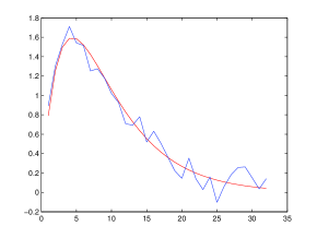
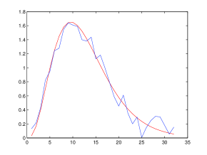
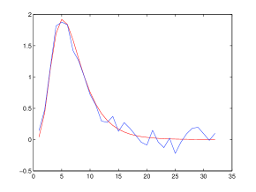
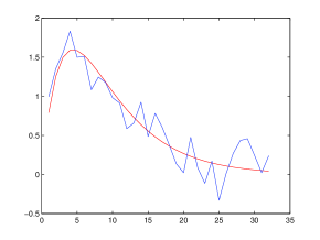
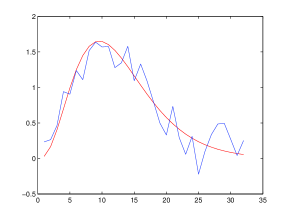
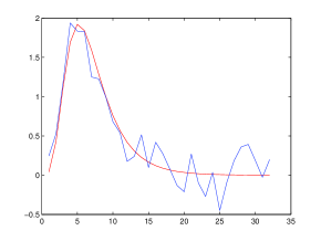
Figure 1: The true function q𝑞q (red) and vector 𝐲𝐲\mathbf{y} (blue) for test functions f1subscript𝑓1f_{1} (left), f2subscript𝑓2f_{2} (middle) and f3subscript𝑓3f_{3} (right) with n=32𝑛32n=32 and σ=0.5𝜎0.5\sigma=0.5 (top) and σ=1𝜎1\sigma=1 (bottom).

In order to evaluate the performance of the procedure suggested in the paper we carried out a limited simulation study. We considered a Laplace convolution equation (9.9) studied above in Section 9.2 with g(x)=exp(x)𝑔𝑥𝑥g(x)=\exp(-x), observation points uniformly spaced on the interval [0;T]0𝑇[0;T] with T=10𝑇10T=10 and n=32𝑛32n=32 or n=64𝑛64n=64 observation points. The choice of the kernel g𝑔g and the sample size are motivated by the fact that Laplace convolution equation with the kernel of this form satisfies the conditions required for application of the wavelet-vaguelette estimator which we use for comparison with our estimator.

We constructed a fixed dictionary of the form 𝒟={φjφlkj,bij,j=1,,p},𝒟formulae-sequencesubscript𝜑𝑗subscript𝜑subscript𝑙subscript𝑘𝑗subscript𝑏subscript𝑖𝑗𝑗1𝑝{\mathcal{D}}=\left\{\varphi_{j}\equiv\varphi_{l_{k_{j}},b_{i_{j}}},\ j=1,\cdots,p\right\}, where φl,bsubscript𝜑𝑙𝑏\varphi_{l,b} are defined in formula (9.13) with lk=ksubscript𝑙𝑘𝑘l_{k}=k, k=0p1𝑘0subscript𝑝1k=0\cdots p_{1}, and bk=0.1ksubscript𝑏𝑘0.1𝑘b_{k}=0.1\ k, k=1,,p2𝑘1subscript𝑝2k=1,\cdots,p_{2}. We chose p1=10subscript𝑝110p_{1}=10, p2=40subscript𝑝240p_{2}=40, giving the total of p=p1p2=400𝑝subscript𝑝1subscript𝑝2400p=p_{1}p_{2}=400 dictionary elements. We evaluated the dictionary functions on a fine grid, scaled them to have unit norms and formed matrix 𝐖𝐖\mathbf{W} with columns 𝝋jsubscript𝝋𝑗\mbox{$\varphi$}_{j}, j=1,,p𝑗1𝑝j=1,\cdots,p. Vector 𝐲𝐲\mathbf{y} was calculated at n𝑛n observation points as 𝐲=𝐪+n1/2σ𝝃𝐲𝐪superscript𝑛12𝜎𝝃\mathbf{y}=\mathbf{q}+n^{-1/2}\,\sigma\mbox{$\xi$} where 𝝃n𝝃superscript𝑛\mbox{$\xi$}\in{\mathbb{R}}^{n} is a standard normal vector.

In order to generate operator 𝐐𝐐\mathbf{Q} we sampled functions f𝑓f and g𝑔g on a fine grid. Matrix 𝐐𝐐\mathbf{Q} was constructed so that it carried out numerical integration in formula (9.9) for 0xT0𝑥𝑇0\leq x\leq T, i.e., q=Qf𝑞𝑄𝑓q=Qf. We obtained matrix 𝚿𝚿\Psi of the inverse images by the numerical solution of the exact equation 𝐐𝚿=𝐖superscript𝐐𝚿𝐖\mathbf{Q}^{*}\mbox{$\Psi$}=\mathbf{W}. We estimated vector 𝜷𝜷\beta with elements (4.4) by 𝜷^=𝚿T𝐲^𝜷superscript𝚿𝑇𝐲\hat{\mbox{$\beta$}}=\mbox{$\Psi$}^{T}\mathbf{y} and solve optimization problem (4.9). For implementation of minimization in (4.9), we used function LassoWeighted in SPAMS MatLab toolbox [30]. We calculated αmaxsubscript𝛼\alpha_{\max} as the value of the Lasso parameter that guarantees that all coefficients in the model vanish. We created a grid of the values of αk=αmaxk/Nsubscript𝛼𝑘subscript𝛼𝑘𝑁\alpha_{k}=\alpha_{\max}*k/N, i=1,,N𝑖1𝑁i=1,\cdots,N, with N=200𝑁200N=200. As a result, we obtained a collection of estimators 𝜽^=𝜽^(αk)^𝜽^𝜽subscript𝛼𝑘\widehat{\mbox{$\theta$}}=\widehat{\mbox{$\theta$}}(\alpha_{k}). Finally, we chose α=αopt=αk~𝛼subscript𝛼𝑜𝑝𝑡subscript𝛼~𝑘\alpha=\alpha_{opt}=\alpha_{\widetilde{k}} where where k~=argmink𝐟^(αk)𝐟||\widetilde{k}=\arg\min_{k}\|\hat{\mathbf{f}}(\alpha_{k})-\mathbf{f}||.

Refer to caption  Refer to caption  Refer to caption
Figure 2: Four estimators of function f𝑓f (red) with n=64𝑛64n=64: the Lasso estimator 𝐟^Las,cvsubscript^𝐟𝐿𝑎𝑠𝑐𝑣\hat{\mathbf{f}}_{Las,cv} with Lasso parameter α^^𝛼\hat{\alpha} derived by cross validation (blue), the SVD estimator 𝐟^SVDsubscript^𝐟𝑆𝑉𝐷\hat{\mathbf{f}}_{SVD} (black), the Laguerre function estimator 𝐟^Lagsubscript^𝐟𝐿𝑎𝑔\hat{\mathbf{f}}_{Lag} (green) and the wavelet-vaguelette estimator 𝐟^wavsubscript^𝐟𝑤𝑎𝑣\hat{\mathbf{f}}_{wav} (magenta). Top row: σ=0.5𝜎0.5\sigma=0.5. Bottom row: σ=1𝜎1\sigma=1.

We constructed Lasso estimator 𝐟^Las,opt=𝐖𝜽^(αk~)subscript^𝐟𝐿𝑎𝑠𝑜𝑝𝑡𝐖^𝜽subscript𝛼~𝑘\hat{\mathbf{f}}_{Las,opt}=\mathbf{W}\widehat{\mbox{$\theta$}}(\alpha_{\widetilde{k}}) with the optimal choice of the penalty parameter. In practice, 𝐟𝐟\mathbf{f} is unavailable and parameter α𝛼\alpha is chosen by cross validation. In particular, we estimated q𝑞q by a projection estimator 𝐪^^𝐪\widehat{\mathbf{q}} using Laguerre functions basis and the vector of observations y𝑦y and chose α=α^=αk^𝛼^𝛼subscript𝛼^𝑘\alpha=\hat{\alpha}=\alpha_{\widehat{k}}. Here

k^=argmink𝐖𝜽^(αk)𝐪^22+2σ2n1p^k^𝑘subscript𝑘subscriptsuperscriptnorm𝐖^𝜽subscript𝛼𝑘^𝐪222superscript𝜎2superscript𝑛1subscript^𝑝𝑘\widehat{k}=\arg\min_{k}\|\mathbf{W}\widehat{\mbox{$\theta$}}(\alpha_{k})-\hat{\mathbf{q}}\|^{2}_{2}+2\sigma^{2}n^{-1}\hat{p}_{k}

where p^ksubscript^𝑝𝑘\hat{p}_{k} is the number of nonzero components of 𝜽^(αk)^𝜽subscript𝛼𝑘\widehat{\mbox{$\theta$}}(\alpha_{k}) which, in our case, coincided with the dimension of the linear space 𝐖𝜽^(αk)𝐖^𝜽subscript𝛼𝑘\mathbf{W}\widehat{\mbox{$\theta$}}(\alpha_{k}). At last, we set 𝐟^Las,cv=𝐟^(αk^)subscript^𝐟𝐿𝑎𝑠𝑐𝑣^𝐟subscript𝛼^𝑘\hat{\mathbf{f}}_{Las,cv}=\hat{\mathbf{f}}(\alpha_{\widehat{k}}).

We compared the Lasso estimators 𝐟^Las,optsubscript^𝐟𝐿𝑎𝑠𝑜𝑝𝑡\hat{\mathbf{f}}_{Las,opt} and 𝐟^Las,cvsubscript^𝐟𝐿𝑎𝑠𝑐𝑣\hat{\mathbf{f}}_{Las,cv} with the estimators 𝐟^SVDsubscript^𝐟𝑆𝑉𝐷\hat{\mathbf{f}}_{SVD}, 𝐟^wavsubscript^𝐟𝑤𝑎𝑣\hat{\mathbf{f}}_{wav} and 𝐟^Lagsubscript^𝐟𝐿𝑎𝑔\hat{\mathbf{f}}_{Lag} where 𝐟^SVDsubscript^𝐟𝑆𝑉𝐷\hat{\mathbf{f}}_{SVD} is recovered by the singular value decomposition (SVD), 𝐟^wavsubscript^𝐟𝑤𝑎𝑣\hat{\mathbf{f}}_{wav} is the wavelet-vaguelette estimator obtained by using Daubechies wavelet of degree 6 and 𝐟^Lagsubscript^𝐟𝐿𝑎𝑔\hat{\mathbf{f}}_{Lag} is constructed by expanding the unknown function f𝑓f over the system of Laguerre functions (9.12) with a=1/2𝑎12a=1/2. The Laguerre functions dictionary has been proven to be extremely efficient for Laplace deconvolution (see, e.g., [12] and [35]). We used Kssubscript𝐾𝑠K_{s} eigenbasis functions for SVD, KLsubscript𝐾𝐿K_{L} Laguerre functions for the Laguerre function solution and hard thresholding with threshold ΛΛ\Lambda for the wavelet-vaguelette estimator. In order to simplify our numerical work, for all three estimators, the SVD, the wavelet-vaguelette and the Laguerre functions based estimator, we used the “ideal” parameter choices, selecting parameters Kssubscript𝐾𝑠K_{s}, KLsubscript𝐾𝐿K_{L} and ΛΛ\Lambda by minimizing the difference between the respective estimators and the true function 𝐟𝐟\mathbf{f} which is unavailable in a real life setting. Therefore, precision of the three competitive estimators is somewhat higher than it would be in a real life situation where parameters of the methods have to be estimated from data.
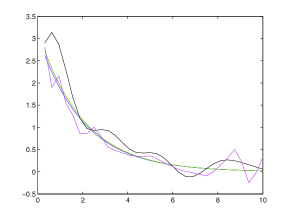
Refer to caption  Refer to caption  Refer to caption
Figure 3: Four estimators of function f𝑓f (red) with n=32𝑛32n=32: the Lasso estimator 𝐟^Las,cvsubscript^𝐟𝐿𝑎𝑠𝑐𝑣\hat{\mathbf{f}}_{Las,cv} with Lasso parameter α^^𝛼\hat{\alpha} derived by cross validation (blue), the SVD estimator 𝐟^SVDsubscript^𝐟𝑆𝑉𝐷\hat{\mathbf{f}}_{SVD} (black), the Laguerre function estimator 𝐟^Lagsubscript^𝐟𝐿𝑎𝑔\hat{\mathbf{f}}_{Lag} (green) and the wavelet-vaguelette estimator 𝐟^wavsubscript^𝐟𝑤𝑎𝑣\hat{\mathbf{f}}_{wav} (magenta). Top row: σ=0.5𝜎0.5\sigma=0.5. Bottom row: σ=1𝜎1\sigma=1.

We carried out numerical experiments with two sample sizes, n=32𝑛32n=32 and n=64𝑛64n=64, three noise levels, σ=0.25𝜎0.25\sigma=0.25 (low noise level), σ=0.5𝜎0.5\sigma=0.5 (medium noise level) and σ=1𝜎1\sigma=1 (high noise level), and several test functions. In particular, we chose three test functions, f1(x)=Cexp(x/2)subscript𝑓1𝑥𝐶𝑥2f_{1}(x)=C\exp(-x/2), f2(x)=Cx2exp(x)subscript𝑓2𝑥𝐶superscript𝑥2𝑥f_{2}(x)=Cx^{2}*\exp(-x) and f3(x)=Cx4exp(4x)subscript𝑓3𝑥𝐶superscript𝑥44𝑥f_{3}(x)=Cx^{4}*\exp(-4*x), where all functions were scaled to have the unit L2superscript𝐿2L^{2} norms. The first test function is easy to estimate and it benefits 𝐟^Lagsubscript^𝐟𝐿𝑎𝑔\hat{\mathbf{f}}_{Lag} since it coincides with the first function of the Laguerre basis. The second function is moderately hard and the last function is the most difficult to estimate.
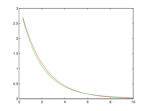
Refer to caption  Refer to caption  Refer to caption
Figure 4: Lasso estimators of function f𝑓f (red) with n=32𝑛32n=32: the Lasso estimator 𝐟^Las,cvsubscript^𝐟𝐿𝑎𝑠𝑐𝑣\hat{\mathbf{f}}_{Las,cv} (blue) with Lasso parameter α=α^𝛼^𝛼\alpha=\hat{\alpha} derived by cross validation and the Lasso estimator 𝐟^Las,optsubscript^𝐟𝐿𝑎𝑠𝑜𝑝𝑡\hat{\mathbf{f}}_{Las,opt} (green) with the optimal choice of Lasso parameter.

Figure 1 displays the true functions q𝑞q and vector 𝐲𝐲\mathbf{y} with n=32𝑛32n=32 and σ=0.5𝜎0.5\sigma=0.5 and σ=1𝜎1\sigma=1, respectively, for these three cases. Figures 2 and 3 show the true function f𝑓f (red) and its four estimators for, respectively, n=64𝑛64n=64 and n=32𝑛32n=32: the Lasso estimator 𝐟^Las,cvsubscript^𝐟𝐿𝑎𝑠𝑐𝑣\hat{\mathbf{f}}_{Las,cv} with the Lasso parameter derived by cross validation (blue), the SVD estimator (black), the Laguerre function based estimator (green) and the wavelet-vaguelette estimator (magenta). Finally, Figure 4 exhibits the Lasso estimators 𝐟^Las,optsubscript^𝐟𝐿𝑎𝑠𝑜𝑝𝑡\hat{\mathbf{f}}_{Las,opt} with the optimal choice of parameter α𝛼\alpha, and 𝐟^Las,cvsubscript^𝐟𝐿𝑎𝑠𝑐𝑣\hat{\mathbf{f}}_{Las,cv}, with parameter α𝛼\alpha obtained using cross-validation, when n=32𝑛32n=32 and σ=1𝜎1\sigma=1 for the three choices of test functions. Figure 4 as well as Table 1 below show that the estimators 𝐟^Las,optsubscript^𝐟𝐿𝑎𝑠𝑜𝑝𝑡\hat{\mathbf{f}}_{Las,opt} and 𝐟^Las,cvsubscript^𝐟𝐿𝑎𝑠𝑐𝑣\hat{\mathbf{f}}_{Las,cv} (and, consequently, their errors) are very close to each other.

Table 1 below compares the accuracy of the Lasso estimators with the three competitive estimators: the SVD estimator, the wavelet-vaguelette estimator and Laguerre functions expansion based estimator described above. Precision of an estimator 𝐟^^𝐟\hat{\mathbf{f}} is measured by the estimated L2superscript𝐿2L^{2}-norm R(𝐟^)=n1/2𝐟^𝐟2𝑅^𝐟superscript𝑛12subscriptnorm^𝐟𝐟2R(\hat{\mathbf{f}})=n^{-1/2}\,\|\hat{\mathbf{f}}-\mathbf{f}\|_{2} of the difference between the estimator 𝐟^^𝐟\hat{\mathbf{f}} and the true vector 𝐟𝐟\mathbf{f} averaged over 50 simulation runs (with the standard deviations listed in parentheses). Columns 1 and 2 present, respectively, the average MSEs of the Lasso estimators 𝐟^Las,optsubscript^𝐟𝐿𝑎𝑠𝑜𝑝𝑡\hat{\mathbf{f}}_{Las,opt} with the optimal choice of parameter α𝛼\alpha, and 𝐟^Las,cvsubscript^𝐟𝐿𝑎𝑠𝑐𝑣\hat{\mathbf{f}}_{Las,cv}, with parameter α𝛼\alpha obtained using cross-validation. Columns 3–5 display the average MSEs of the SVD estimator 𝐟^SVDsubscript^𝐟𝑆𝑉𝐷\hat{\mathbf{f}}_{SVD}, the wavelet-vaguelette estimator 𝐟^wavsubscript^𝐟𝑤𝑎𝑣\hat{\mathbf{f}}_{wav} and the Laguerre functions based estimator 𝐟^Lagsubscript^𝐟𝐿𝑎𝑔\hat{\mathbf{f}}_{Lag}.

The accuracies of the Lasso estimators, the SVD estimators,
the wavelet-vaguelette estimator and the Laguerre functions
based estimators averaged over 50 simulation runs
Method 𝐟^Las,optsubscript^𝐟𝐿𝑎𝑠𝑜𝑝𝑡\hat{\mathbf{f}}_{Las,opt} 𝐟^Las,cvsubscript^𝐟𝐿𝑎𝑠𝑐𝑣\hat{\mathbf{f}}_{Las,cv} 𝐟^SVDsubscript^𝐟𝑆𝑉𝐷\hat{\mathbf{f}}_{SVD} 𝐟^wavsubscript^𝐟𝑤𝑎𝑣\hat{\mathbf{f}}_{wav} 𝐟^Lagsubscript^𝐟𝐿𝑎𝑔\hat{\mathbf{f}}_{Lag}
f(x)=exp(x/2)𝑓𝑥𝑥2f(x)=\exp(-x/2) 0.019795 0.021403 0.094387 0.106268 0.003351
σ=0.25𝜎0.25\sigma=0.25, n=64𝑛64n=64 (0.009531) (0.011563) (0.004851) (0.014351) (0.002870)
f(x)=exp(x/2)𝑓𝑥𝑥2f(x)=\exp(-x/2) 0.032464 0.038243 0.117718 0.191543 0.006703
σ=0.5𝜎0.5\sigma=0.5, n=64𝑛64n=64 (0.017158) (0.020279) (0.009292) (0.054438) (0.005740)
f(x)=exp(x/2)𝑓𝑥𝑥2f(x)=\exp(-x/2) 0.058041 0.067571 0.153829 0.345168 0.013406
σ=1𝜎1\sigma=1, n=64𝑛64n=64 (0.031136) (0.034896) (0.017815) (0.048606) (0.011481)
f(x)=exp(x/2)𝑓𝑥𝑥2f(x)=\exp(-x/2) 0.045767 0.048617 0.159040 0.118117 0.007028
σ=0.25𝜎0.25\sigma=0.25, n=32𝑛32n=32 (0.016654) (0.016153) (0.007930) (0.020318) (0.005496)
f(x)=exp(x/2)𝑓𝑥𝑥2f(x)=\exp(-x/2) 0.062453 0.066710 0.185882 0.187190 0.014057
σ=0.5𝜎0.5\sigma=0.5, n=32𝑛32n=32 (0.028558) (0.028691) (0.015800) (0.038958) (0.010991)
f(x)=exp(x/2)𝑓𝑥𝑥2f(x)=\exp(-x/2) 0.100206 0.113646 0.233622 0.363585 0.028113
σ=1𝜎1\sigma=1, n=32𝑛32n=32 (0.049762) (0.050458) (0.027932) (0.077715) (0.021983)
f(x)=x2exp(x)𝑓𝑥superscript𝑥2𝑥f(x)=x^{2}\exp(-x) 0.015049 0.016560 0.062621 0.090289 0.018849
σ=0.25𝜎0.25\sigma=0.25, n=64𝑛64n=64 (0.005400) (0.005958) (0.003635) (0.005864) (0.004934)
f(x)=x2exp(x)𝑓𝑥superscript𝑥2𝑥f(x)=x^{2}\exp(-x) 0.027391 0.034609 0.076469 0.100841 0.034744
σ=0.5𝜎0.5\sigma=0.5, n=64𝑛64n=64 (0.010565) (0.016077) (0.007881) (0.009059) (0.010220)
f(x)=x2exp(x)𝑓𝑥superscript𝑥2𝑥f(x)=x^{2}\exp(-x) 0.051201 0.061012 0.103803 0.143001 0.064760
σ=1𝜎1\sigma=1, n=64𝑛64n=64 (0.019715) (0.022200) (0.012547) (0.027588) (0.019903)
f(x)=x2exp(x)𝑓𝑥superscript𝑥2𝑥f(x)=x^{2}\exp(-x) 0.028626 0.031445 0.117126 0.162770 0.035111
σ=0.25𝜎0.25\sigma=0.25, n=32𝑛32n=32 (0.012081) (0.013028) (0.005548) (0.009057) (0.011335)
f(x)=x2exp(x)𝑓𝑥superscript𝑥2𝑥f(x)=x^{2}\exp(-x) 0.046965 0.053782 0.136472 0.181601 0.062855
σ=0.5𝜎0.5\sigma=0.5, n=32𝑛32n=32 (0.020748) (0.025215) (0.012993) (0.019603) (0.017499)
f(x)=x2exp(x)𝑓𝑥superscript𝑥2𝑥f(x)=x^{2}\exp(-x) 0.083337 0.095734 0.174761 0.232028 0.104431
σ=1𝜎1\sigma=1, n=32𝑛32n=32 (0.036605) (0.038061) (0.024907) (0.040098) (0.022430)
f(x)=x4exp(4x)𝑓𝑥superscript𝑥44𝑥f(x)=x^{4}\exp(-4x) 0.025236 0.026016 0.095819 0.150802 0.045406
σ=0.25𝜎0.25\sigma=0.25, n=64𝑛64n=64 (0.011729) (0.011917) (0.004939) (0.015667) (0.010733)
f(x)=x4exp(4x)𝑓𝑥superscript𝑥44𝑥f(x)=x^{4}\exp(-4x) 0.040865 0.046998 0.120739 0.211242 0.074079
σ=0.5𝜎0.5\sigma=0.5, n=64𝑛64n=64 (0.021255) (0.025032) (0.012737) (0.035823) (0.018005)
f(x)=x4exp(4x)𝑓𝑥superscript𝑥44𝑥f(x)=x^{4}\exp(-4x) 0.070826 0.085365 0.176209 0.281932 0.126000
σ=1𝜎1\sigma=1, n=64𝑛64n=64 (0.038718) (0.040451) (0.024383) (0.025090) (0.031723)
f(x)=x4exp(4x)𝑓𝑥superscript𝑥44𝑥f(x)=x^{4}\exp(-4x) 0.051191 0.052743 0.180319 0.266600 0.071385
σ=0.25𝜎0.25\sigma=0.25, n=32𝑛32n=32 (0.024067) (0.023798) (0.008549) (0.021389) (0.019737)
f(x)=x4exp(4x)𝑓𝑥superscript𝑥44𝑥f(x)=x^{4}\exp(-4x) 0.071112 0.077483 0.217531 0.311368 0.119478
σ=0.5𝜎0.5\sigma=0.5, n=32𝑛32n=32 (0.041662) (0.041242) (0.023746) (0.024043) (0.030617)
f(x)=x4exp(4x)𝑓𝑥superscript𝑥44𝑥f(x)=x^{4}\exp(-4x) 0.110801 0.128099 0.300436 0.360937 0.204710
σ=1𝜎1\sigma=1, n=32𝑛32n=32 (0.067313) (0.064436) (0.049631) (0.036405) (0.047348)
Table 1: The average values (evaluated over 50 simulation runs) of the errors of the Lasso estimators 𝐟^Las,optsubscript^𝐟𝐿𝑎𝑠𝑜𝑝𝑡\hat{\mathbf{f}}_{Las,opt} and 𝐟^Las,cvsubscript^𝐟𝐿𝑎𝑠𝑐𝑣\hat{\mathbf{f}}_{Las,cv} the SVD estimator 𝐟^SVDsubscript^𝐟𝑆𝑉𝐷\hat{\mathbf{f}}_{SVD}, the wavelet-vaguelette estimator 𝐟^wavsubscript^𝐟𝑤𝑎𝑣\hat{\mathbf{f}}_{wav} and the Laguerre function estimator 𝐟^Lagsubscript^𝐟𝐿𝑎𝑔\hat{\mathbf{f}}_{Lag}. Standard deviations of the errors are listed in the parentheses.

Results in Table 1 confirm that procedure developed in the paper has good computational properties. Indeed, in our simulations, even with the penalty parameter obtained via cross validation, Lasso yields better precision than both the SVD and the wavelet-vaguelette estimators 𝐟^SVDsubscript^𝐟𝑆𝑉𝐷\hat{\mathbf{f}}_{SVD} and 𝐟^wavsubscript^𝐟𝑤𝑎𝑣\hat{\mathbf{f}}_{wav} with hand-chosen parameter values. For the first test functions, 𝐟^Lagsubscript^𝐟𝐿𝑎𝑔\hat{\mathbf{f}}_{Lag} is more accurate since the Laguerre basis contains the function of interest and, due to orthonormality of the basis, one does not have to pay a price for selecting the correct dictionary functions. However, for the first test function, both 𝐟^Lassosubscript^𝐟𝐿𝑎𝑠𝑠𝑜\hat{\mathbf{f}}_{Lasso} and 𝐟^Lagsubscript^𝐟𝐿𝑎𝑔\hat{\mathbf{f}}_{Lag} produce almost a perfect reconstruction as the left panels of Figures 2 and 3 demonstrate. For the second and the third test functions, Lasso exhibits better precision than its competitors in spite of the fact that we used a fully adaptive Lasso estimator (the choice of Lasso parameter was data-driven) while, for all three other methods, parameters were determined on the basis of the true function f𝑓f which is not known in practice.

One can easily see that the SVD estimators have relatively high errors. The latter can be explained by the fact that the eigenfunctions of the Laplace convolution operator exhibit oscillatory behavior (which can be see on Figures 2 and 3), so, they require a large number of elements for representation of f𝑓f. The large errors of the wavelet-vaguelette estimator are partially due to using periodic wavelets defined on a finite interval while estimating non-periodic functions. Consequently, the wavelet-vaguelette estimator exhibits strong boundary effects since we did not carry out the boundary correction.

11 Discussion

In the present paper, we consider application of Lasso to a general linear inverse problem. The approach is based on inverting of each of the dictionary functions and matching the resulting expansion to the true function f𝑓f. We investigate the white noise formulation of the problem and further extend the theory to the case of discrete observations with Gaussian or sub-Gaussian noise. In addition, we explain how this methodology can be used when the inverse images of the dictionary functions are replaced by their approximate versions. We also show how the technique suggested in the paper can be extended to the problem of estimation of a mixing density in a continuous mixture.

Using an example of the Laplace convolution equation, we study performance of the Lasso-based estimators via simulations and compare their precisions with the SVD estimators, the wavelet-vaguelette estimators and the estimators based on the expansion of the unknown function via the Laguerre functions basis. We show that as long as the function of interest f𝑓f has a compact representation in the overcomplete dictionary, the Lasso estimator yields satisfactory reconstruction. Indeed, in our simulation study, it demonstrates comparable or better precision than its competitors.

Although in the paper we assume that the linear operator Q𝑄Q is completely known, the theory can be extended to the case when operator Q𝑄Q is measured with error or is estimated from the data. The advantage of the approach of the paper is that it naturally partitions the problem of solution of a linear inverse problem with a noisy operator and a right hand side measured with error into two easier problems: solution of an inverse linear problem with the noisy operator and completely known right hand side, and estimation of the linear functional of the right hand side on the basis of its noisy version. However, solution of general linear ill-posed problems with noisy operators lie outside the scope of the present paper and will be treated in future.

Acknowledgments

Marianna Pensky was partially supported by National Science Foundation (NSF), grants DMS-1106564 and DMS-1407475. The author would also like to thank SAMSI for providing support which allowed the author’s participation in the 2013-14 LDHD program which was instrumental for writing this paper.

12 Proofs

Validity of Theorems 14 rely on the following Lemma, the proof of which follows the lines of reasoning in [14]. However, since we are interested in weighted Lasso and allow for non-centered errors, for completeness, we provide the proof of the Lemma below.

Lemma 3

Let f𝑓f be the true function and f𝛉subscript𝑓𝛉f_{{\mbox{$\theta$}}} be its projection onto the linear span of the dictionary 𝒫subscript𝒫{\mathcal{L}}_{{\mathcal{P}}}. Consider solution of the weighted Lasso problem (4.8) with 𝚽=𝐖T𝐖𝚽superscript𝐖𝑇𝐖\mbox{$\Phi$}=\mathbf{W}^{T}\mathbf{W}, 𝛃=𝚽𝛉𝛃𝚽𝛉\mbox{$\beta$}=\mbox{$\Phi$}\mbox{$\theta$} and 𝛃^=𝐖T𝛄^𝛃superscript𝐖𝑇𝛄\widehat{\mbox{$\beta$}}=\mathbf{W}^{T}\mbox{$\gamma$}. Let

𝜷^=𝜷+ϵ𝚼𝛈+𝐡,𝜼,𝐡p,formulae-sequence^𝜷𝜷italic-ϵ𝚼𝛈𝐡𝜼𝐡superscript𝑝\widehat{\mbox{$\beta$}}=\mbox{$\beta$}+\sqrt{\epsilon}\mbox{$\Upsilon$}\mbox{$\eta$}+\mathbf{h},\quad\mbox{$\eta$},\mathbf{h}\in{\mathbb{R}}^{p}, (12.1)

where 𝔼𝛈=0𝔼𝛈0{\mathbb{E}}\mbox{$\eta$}=0 and components ηjsubscript𝜂𝑗\eta_{j} of 𝛈𝛈\eta are sub-Gaussian random variables satisfying, for some K>0𝐾0K>0 and any t𝑡t,

(|ηi|>t)2exp(t2/K2).subscript𝜂𝑖𝑡2superscript𝑡2superscript𝐾2{\mathbb{P}}\left(|\eta_{i}|>t\right)\leq 2\,\exp(-t^{2}/K^{2}). (12.2)

Choose τ>0𝜏0\tau>0 and denote

Ch=max1jp[|hj|νjϵlogp],Cα=Kτ+1+Ch.formulae-sequencesubscript𝐶subscript1𝑗𝑝subscript𝑗subscript𝜈𝑗italic-ϵ𝑝subscript𝐶𝛼𝐾𝜏1subscript𝐶C_{h}=\max_{1\leq j\leq p}\left[\frac{|h_{j}|}{\nu_{j}\,\sqrt{\epsilon\,\log p}}\right],\quad\quad C_{\alpha}=K\sqrt{\tau+1}+C_{h}. (12.3)

If α0=Cαϵlogpsubscript𝛼0subscript𝐶𝛼italic-ϵ𝑝\alpha_{0}=C_{\alpha}\sqrt{\epsilon\log p}, then for any τ>0𝜏0\tau>0 and any αα0𝛼subscript𝛼0\alpha\geq\alpha_{0}, with probability at least 12pτ12superscript𝑝𝜏1-2p^{-\tau}, one has

f𝜽^f22inf𝐭[f𝐭f22+4α𝚼𝐭1].superscriptsubscriptnormsubscript𝑓^𝜽𝑓22subscriptinfimum𝐭delimited-[]superscriptsubscriptnormsubscript𝑓𝐭𝑓224𝛼subscriptnorm𝚼𝐭1\|f_{\widehat{\mbox{$\theta$}}}-f\|_{2}^{2}\leq\inf_{\mathbf{t}}\left[\|f_{\mathbf{t}}-f\|_{2}^{2}+4\alpha\|\mbox{$\Upsilon$}\mathbf{t}\|_{1}\right]. (12.4)

Moreover, if Assumption A holds and α=α0(μ+1)/(μ1)𝛼subscript𝛼0𝜇1𝜇1\alpha=\alpha_{0}(\mu+1)/(\mu-1), then, for any τ>0𝜏0\tau>0 with probability at least 12pτ12superscript𝑝𝜏1-2p^{-\tau}, one has

f𝜽^f22inf𝐭,J𝒫[f𝐭f22+4α(𝚼𝐭)Jc1+4Cα2μ2(μ1)2κ2(μ,J)ϵlogpjJνj2].superscriptsubscriptnormsubscript𝑓^𝜽𝑓22subscriptinfimum𝐭𝐽𝒫delimited-[]superscriptsubscriptnormsubscript𝑓𝐭𝑓224𝛼subscriptnormsubscript𝚼𝐭superscript𝐽𝑐14superscriptsubscript𝐶𝛼2superscript𝜇2superscript𝜇12superscript𝜅2𝜇𝐽italic-ϵ𝑝subscript𝑗𝐽superscriptsubscript𝜈𝑗2\|f_{\widehat{\mbox{$\theta$}}}-f\|_{2}^{2}\leq\inf_{\mathbf{t},J\subseteq{\mathcal{P}}}\left[\|f_{\mathbf{t}}-f\|_{2}^{2}+4\alpha\|(\mbox{$\Upsilon$}\mathbf{t})_{{J^{c}}}\|_{1}+\frac{4C_{\alpha}^{2}\mu^{2}}{(\mu-1)^{2}\kappa^{2}(\mu,J)}\epsilon\log p\ \sum_{j\in J}\nu_{j}^{2}\right]. (12.5)

Proof of Lemma 3 . Following Dalalyan et al. (2014), by K-K-T condition, we derive for any 𝐭p𝐭superscript𝑝\mathbf{t}\in{\mathbb{R}}^{p}

𝜽^T(𝜷^𝚽𝜽^)superscript^𝜽𝑇^𝜷𝚽^𝜽\displaystyle\widehat{\mbox{$\theta$}}^{T}(\widehat{\mbox{$\beta$}}-\mbox{$\Phi$}\widehat{\mbox{$\theta$}}) =\displaystyle= α𝚼𝜽^1,𝐭T(𝜷^𝚽𝜽^)α𝚼𝐭1,𝛼subscriptnorm𝚼^𝜽1superscript𝐭𝑇^𝜷𝚽^𝜽𝛼subscriptnorm𝚼𝐭1\displaystyle\alpha\|\mbox{$\Upsilon$}\widehat{\mbox{$\theta$}}\|_{1},\quad\mathbf{t}^{T}(\widehat{\mbox{$\beta$}}-\mbox{$\Phi$}\widehat{\mbox{$\theta$}})\leq\alpha\|\mbox{$\Upsilon$}\mathbf{t}\|_{1},

so that, subtracting the first line from the second, we obtain

(𝜽^𝐭)T(𝚽𝜽^𝜷^)α(𝚼𝐭1𝚼𝜽^1).superscript^𝜽𝐭𝑇𝚽^𝜽^𝜷𝛼subscriptnorm𝚼𝐭1subscriptnorm𝚼^𝜽1(\widehat{\mbox{$\theta$}}-\mathbf{t})^{T}(\mbox{$\Phi$}\widehat{\mbox{$\theta$}}-\widehat{\mbox{$\beta$}})\leq\alpha\left(\|\mbox{$\Upsilon$}\mathbf{t}\|_{1}-\|\mbox{$\Upsilon$}\widehat{\mbox{$\theta$}}\|_{1}\right). (12.6)

Since 𝚽𝜽=𝜷𝚽𝜽𝜷\mbox{$\Phi$}\mbox{$\theta$}=\mbox{$\beta$}, (12.6) yields

(𝜽^𝐭)T𝚽(𝜽^𝜽)ϵ(𝜽^𝐭)T𝚼𝜼+(𝜽^𝐭)T𝐡+α(𝚼𝐭1𝚼𝜽^1)..superscript^𝜽𝐭𝑇𝚽^𝜽𝜽italic-ϵsuperscript^𝜽𝐭𝑇𝚼𝜼superscript^𝜽𝐭𝑇𝐡𝛼subscriptnorm𝚼𝐭1subscriptnorm𝚼^𝜽1(\widehat{\mbox{$\theta$}}-\mathbf{t})^{T}\mbox{$\Phi$}(\widehat{\mbox{$\theta$}}-\mbox{$\theta$})\leq\sqrt{\epsilon}(\widehat{\mbox{$\theta$}}-\mathbf{t})^{T}\mbox{$\Upsilon$}\mbox{$\eta$}+(\widehat{\mbox{$\theta$}}-\mathbf{t})^{T}\mathbf{h}+\alpha\left(\|\mbox{$\Upsilon$}\mathbf{t}\|_{1}-\|\mbox{$\Upsilon$}\widehat{\mbox{$\theta$}}\|_{1}\right)..

Since for any 𝐮,𝐯p𝐮𝐯superscript𝑝\mathbf{u},\mathbf{v}\in{\mathbb{R}}^{p} one has 𝐯T𝚽𝐮=12[𝐯T𝚽𝐯+𝐮T𝚽𝐮(𝐯𝐮)T𝚽(𝐯𝐮)],superscript𝐯𝑇𝚽𝐮12delimited-[]superscript𝐯𝑇𝚽𝐯superscript𝐮𝑇𝚽𝐮superscript𝐯𝐮𝑇𝚽𝐯𝐮\mathbf{v}^{T}\mbox{$\Phi$}\mathbf{u}=\frac{1}{2}\left[\mathbf{v}^{T}\mbox{$\Phi$}\mathbf{v}+\mathbf{u}^{T}\mbox{$\Phi$}\mathbf{u}-(\mathbf{v}-\mathbf{u})^{T}\mbox{$\Phi$}(\mathbf{v}-\mathbf{u})\right], choosing 𝐯=𝜽^𝐭𝐯^𝜽𝐭\mathbf{v}=\widehat{\mbox{$\theta$}}-\mathbf{t} and 𝐮=𝜽^𝜽𝐮^𝜽𝜽\mathbf{u}=\widehat{\mbox{$\theta$}}-\mbox{$\theta$} and observing that for any 𝐭𝐭\mathbf{t} (and, in particular, for 𝐭=𝜽^𝐭^𝜽\mathbf{t}=\widehat{\mbox{$\theta$}}), f𝐭f22=(𝐭𝜽)T𝚽(𝐭𝜽)+f𝐭f22superscriptsubscriptnormsubscript𝑓𝐭𝑓22superscript𝐭𝜽𝑇𝚽𝐭𝜽superscriptsubscriptnormsubscript𝑓𝐭𝑓22\|f_{\mathbf{t}}-f\|_{2}^{2}=(\mathbf{t}-\mbox{$\theta$})^{T}\mbox{$\Phi$}(\mathbf{t}-\mbox{$\theta$})+\|f_{\mathbf{t}}-f\|_{2}^{2}, for any 𝐭p𝐭superscript𝑝\mathbf{t}\in{\mathbb{R}}^{p}, one obtains

f𝜽^f22+(𝜽^𝐭)T𝚽(𝜽^𝜽)f𝐭f22+ϵ(𝜽^𝐭)T𝚼𝜼+(𝜽^𝐭)T𝐡+2α(𝚼𝐭1𝚼𝜽^1).superscriptsubscriptnormsubscript𝑓^𝜽𝑓22superscript^𝜽𝐭𝑇𝚽^𝜽𝜽superscriptsubscriptnormsubscript𝑓𝐭𝑓22italic-ϵsuperscript^𝜽𝐭𝑇𝚼𝜼superscript^𝜽𝐭𝑇𝐡2𝛼subscriptnorm𝚼𝐭1subscriptnorm𝚼^𝜽1\|f_{\widehat{\mbox{$\theta$}}}-f\|_{2}^{2}+(\widehat{\mbox{$\theta$}}-\mathbf{t})^{T}\mbox{$\Phi$}(\widehat{\mbox{$\theta$}}-\mbox{$\theta$})\leq\|f_{\mathbf{t}}-f\|_{2}^{2}+\sqrt{\epsilon}(\widehat{\mbox{$\theta$}}-\mathbf{t})^{T}\mbox{$\Upsilon$}\mbox{$\eta$}+(\widehat{\mbox{$\theta$}}-\mathbf{t})^{T}\mathbf{h}+2\alpha\left(\|\mbox{$\Upsilon$}\mathbf{t}\|_{1}-\|\mbox{$\Upsilon$}\widehat{\mbox{$\theta$}}\|_{1}\right). (12.7)

By setting t=K(τ+1)logp𝑡𝐾𝜏1𝑝t=K\sqrt{(\tau+1)\log p} in (12.2) and using (12.3), observe that, on the set

Ω={ω:max1jp|ηj|K(τ+1)logp}with(Ω)12pτformulae-sequenceΩconditional-set𝜔subscript1𝑗𝑝subscript𝜂𝑗𝐾𝜏1𝑝withΩ12superscript𝑝𝜏\Omega=\left\{\omega:\max_{1\leq j\leq p}|\eta_{j}|\leq K\sqrt{(\tau+1)\log p}\right\}\quad\mbox{with}\quad{\mathbb{P}}(\Omega)\geq 1-2p^{-\tau} (12.8)

one has

|ϵ(𝜽^𝐭)T𝚼𝜼+(𝜽^𝐭)T𝐡|ϵlogp(Kτ+1+Ch)𝚼(𝜽^𝐭1=α0𝚼(𝜽^𝐭1.\left|\sqrt{\epsilon}(\widehat{\mbox{$\theta$}}-\mathbf{t})^{T}\mbox{$\Upsilon$}\mbox{$\eta$}+(\widehat{\mbox{$\theta$}}-\mathbf{t})^{T}\mathbf{h}\right|\leq\sqrt{\epsilon\,\log p}\,(K\sqrt{\tau+1}+C_{h})\,\|\mbox{$\Upsilon$}(\widehat{\mbox{$\theta$}}-\mathbf{t}\|_{1}=\alpha_{0}\,\|\mbox{$\Upsilon$}(\widehat{\mbox{$\theta$}}-\mathbf{t}\|_{1}.

Combining the last inequality with (12.7), obtain that, for any α>0𝛼0\alpha>0, on the set ΩΩ\Omega,

f𝜽^f2+(𝜽^𝐭)T𝚽(𝜽^𝐭)f𝐭f2+2α(𝚼𝐭1𝚼𝜽^1)+2α0𝚼(𝜽^𝐭)1.superscriptnormsubscript𝑓^𝜽𝑓2superscript^𝜽𝐭𝑇𝚽^𝜽𝐭superscriptnormsubscript𝑓𝐭𝑓22𝛼subscriptnorm𝚼𝐭1subscriptnorm𝚼^𝜽12subscript𝛼0subscriptnorm𝚼^𝜽𝐭1\|f_{\widehat{\mbox{$\theta$}}}-f\|^{2}+(\widehat{\mbox{$\theta$}}-\mathbf{t})^{T}\mbox{$\Phi$}(\widehat{\mbox{$\theta$}}-\mathbf{t})\leq\|f_{\mathbf{t}}-f\|^{2}+2\alpha\left(\|\mbox{$\Upsilon$}\mathbf{t}\|_{1}-\|\mbox{$\Upsilon$}\widehat{\mbox{$\theta$}}\|_{1}\right)+2\alpha_{0}\|\mbox{$\Upsilon$}(\widehat{\mbox{$\theta$}}-\mathbf{t})\|_{1}. (12.9)

Application of inequality 𝚼(𝜽^𝐭)1|𝚼𝐭1+𝚼𝜽^1subscriptnorm𝚼^𝜽𝐭1subscriptdelimited-|‖𝚼𝐭1subscriptnorm𝚼^𝜽1\|\mbox{$\Upsilon$}(\widehat{\mbox{$\theta$}}-\mathbf{t})\|_{1}\leq|\mbox{$\Upsilon$}\mathbf{t}\|_{1}+\|\mbox{$\Upsilon$}\widehat{\mbox{$\theta$}}\|_{1} combined with αα0𝛼subscript𝛼0\alpha\geq\alpha_{0} completes the proof of inequality (12.4).

In order to prove inequality (12.5), denote 𝐝=𝜽^𝐭𝐝^𝜽𝐭\mathbf{d}=\widehat{\mbox{$\theta$}}-\mathbf{t} and observe that, due to |tj||θ^j||θ^jtj|subscript𝑡𝑗subscript^𝜃𝑗subscript^𝜃𝑗subscript𝑡𝑗|t_{j}|-|\widehat{\theta}_{j}|\leq|\widehat{\theta}_{j}-t_{j}| and |θ^j||θ^jtj||tj|subscript^𝜃𝑗subscript^𝜃𝑗subscript𝑡𝑗subscript𝑡𝑗|\widehat{\theta}_{j}|\geq|\widehat{\theta}_{j}-t_{j}|-|t_{j}|, inequality (12.9) implies that, for any set J𝒫𝐽𝒫J\subseteq{\mathcal{P}}, one obtains

f𝜽^f22+𝐝T𝚽𝐝f𝐭f22+4α(𝚼𝐭)Jc1+2(α+α0)(𝚼𝐝)J12(αα0)(𝚼𝐝)Jc1.superscriptsubscriptnormsubscript𝑓^𝜽𝑓22superscript𝐝𝑇𝚽𝐝superscriptsubscriptnormsubscript𝑓𝐭𝑓224𝛼subscriptnormsubscript𝚼𝐭superscript𝐽𝑐12𝛼subscript𝛼0subscriptnormsubscript𝚼𝐝𝐽12𝛼subscript𝛼0subscriptnormsubscript𝚼𝐝superscript𝐽𝑐1\|f_{\widehat{\mbox{$\theta$}}}-f\|_{2}^{2}+\mathbf{d}^{T}\mbox{$\Phi$}\mathbf{d}\leq\|f_{\mathbf{t}}-f\|_{2}^{2}+4\alpha\|(\mbox{$\Upsilon$}\mathbf{t})_{J^{c}}\|_{1}+2(\alpha+\alpha_{0})\|(\mbox{$\Upsilon$}\mathbf{d})_{J}\|_{1}-2(\alpha-\alpha_{0})\|(\mbox{$\Upsilon$}\mathbf{d})_{J^{c}}\|_{1}. (12.10)

Let α=α0(μ+1)/(μ1)𝛼subscript𝛼0𝜇1𝜇1\alpha=\alpha_{0}\,(\mu+1)/(\mu-1), so that (α+α0)/(αα0)=μ𝛼subscript𝛼0𝛼subscript𝛼0𝜇(\alpha+\alpha_{0})/(\alpha-\alpha_{0})=\mu. Now, we consider two possibilities. If μ(𝚼𝐝)J<(𝚼𝐝)Jc𝜇normsubscript𝚼𝐝𝐽normsubscript𝚼𝐝superscript𝐽𝑐\mu\,\|(\mbox{$\Upsilon$}\mathbf{d})_{J}\|<\|(\mbox{$\Upsilon$}\mathbf{d})_{J^{c}}\|, then f𝜽^f22+𝐝T𝚽𝐝f𝐭f22+4α(𝚼𝐭)Jc1superscriptsubscriptnormsubscript𝑓^𝜽𝑓22superscript𝐝𝑇𝚽𝐝superscriptsubscriptnormsubscript𝑓𝐭𝑓224𝛼subscriptnormsubscript𝚼𝐭superscript𝐽𝑐1\|f_{\widehat{\mbox{$\theta$}}}-f\|_{2}^{2}+\mathbf{d}^{T}\mbox{$\Phi$}\mathbf{d}\leq\|f_{\mathbf{t}}-f\|_{2}^{2}+4\alpha\|(\mbox{$\Upsilon$}\mathbf{t})_{J^{c}}\|_{1} and (12.5) is valid. Otherwise, 𝐝𝒥(μ,J)𝐝𝒥𝜇𝐽\mathbf{d}\in{\mathcal{J}}(\mu,J) and, due to compatibility condition (4.13) and inequality 2aba2+b22𝑎𝑏superscript𝑎2superscript𝑏22ab\leq a^{2}+b^{2}, one derives

2(α+α0)(𝚼𝐝)J12(α+α0)Tr(𝚼J2)𝐝T𝚽𝐝/κ(μ,J)𝐝T𝚽𝐝+(α+α0)2Tr(𝚼J2)/κ2(μ,J).2𝛼subscript𝛼0subscriptnormsubscript𝚼𝐝𝐽12𝛼subscript𝛼0Trsuperscriptsubscript𝚼𝐽2superscript𝐝𝑇𝚽𝐝𝜅𝜇𝐽superscript𝐝𝑇𝚽𝐝superscript𝛼subscript𝛼02Trsuperscriptsubscript𝚼𝐽2superscript𝜅2𝜇𝐽2(\alpha+\alpha_{0})\ \|(\mbox{$\Upsilon$}\mathbf{d})_{J}\|_{1}\leq 2(\alpha+\alpha_{0})\ \sqrt{\mbox{Tr}(\mbox{$\Upsilon$}_{J}^{2})\,\mathbf{d}^{T}\mbox{$\Phi$}\mathbf{d}}/\kappa(\mu,J)\leq\mathbf{d}^{T}\mbox{$\Phi$}\mathbf{d}+(\alpha+\alpha_{0})^{2}\,\mbox{Tr}(\mbox{$\Upsilon$}_{J}^{2})/\kappa^{2}(\mu,J).

Plugging the latter into (12.10) and using α=α0(μ+1)/(μ1)𝛼subscript𝛼0𝜇1𝜇1\alpha=\alpha_{0}(\mu+1)/(\mu-1), obtain that (12.5) holds for any 𝐭𝐭\mathbf{t}.

Proof of Theorem 1.   Let 𝜷𝜷\beta and 𝜷^^𝜷\widehat{\mbox{$\beta$}} be the vectors with components 𝜷j=f,φj1subscript𝜷𝑗subscript𝑓subscript𝜑𝑗subscript1\mbox{$\beta$}_{j}=\langle f,\varphi_{j}\rangle_{{\cal H}_{1}} and 𝜷^j=y,ψj2subscript^𝜷𝑗subscript𝑦subscript𝜓𝑗subscript2\widehat{\mbox{$\beta$}}_{j}=\langle y,\psi_{j}\rangle_{{\cal H}_{2}}, j=1,,p𝑗1𝑝j=1,\cdots,p. Then, due to (4.4), one has 𝜷^j=𝜷j+ϵνj𝜼jsubscript^𝜷𝑗subscript𝜷𝑗italic-ϵsubscript𝜈𝑗subscript𝜼𝑗\widehat{\mbox{$\beta$}}_{j}=\mbox{$\beta$}_{j}+\sqrt{\epsilon}\nu_{j}\mbox{$\eta$}_{j} where 𝜼jsubscript𝜼𝑗\mbox{$\eta$}_{j} are standard normal variables. Moreover, if f𝑓f is the true function and f𝜽subscript𝑓𝜽f_{{\mbox{$\theta$}}} is its projection onto the span of the dictionary 𝒫subscript𝒫{\mathcal{L}}_{{\mathcal{P}}}, then, ff𝜽;φj𝑓subscript𝑓𝜽subscript𝜑𝑗\langle f-f_{{\mbox{$\theta$}}};\varphi_{j}\rangle for j=1,,p𝑗1𝑝j=1,\cdots,p, and 𝜷=𝚽𝜽𝜷𝚽𝜽\mbox{$\beta$}=\mbox{$\Phi$}\mbox{$\theta$}. Therefore, validity of Theorem 1 follows from Lemma 3 with K=2𝐾2K=\sqrt{2}, 𝐡=0𝐡0\mathbf{h}=0 and Ch=0subscript𝐶0C_{h}=0 in (12.3).

Proof of Theorem 2.   Validity of (4.14) follows from Lemma 3 with K=2𝐾2K=\sqrt{2}, 𝐡=0𝐡0\mathbf{h}=0 and Ch=0subscript𝐶0C_{h}=0 in (12.3), so that Cα=2(τ+1)subscript𝐶𝛼2𝜏1C_{\alpha}=\sqrt{2(\tau+1)} and K0=2subscript𝐾02K_{0}=2 in (4.14). In order to prove (4.15), choose f𝐭=projJfsubscript𝑓𝐭subscriptprojsubscript𝐽𝑓f_{\mathbf{t}}=\mbox{proj}_{{\mathcal{L}}_{J}}f, so that tj=0subscript𝑡𝑗0t_{j}=0 for jJc𝑗superscript𝐽𝑐j\in{J^{c}}.

Proof of Theorem 3. Note that vector 𝜷^^𝜷\widehat{\mbox{$\beta$}} has components β^j=βj+δj1+δj2subscript^𝛽𝑗subscript𝛽𝑗subscript𝛿𝑗1subscript𝛿𝑗2\widehat{\beta}_{j}=\beta_{j}+\delta_{j1}+\delta_{j2}, j=1,,p𝑗1𝑝j=1,\cdots,p, where

δj1subscript𝛿𝑗1\displaystyle\delta_{j1} =\displaystyle= i=1nξiψj(xi)Δxi,superscriptsubscript𝑖1𝑛subscript𝜉𝑖subscript𝜓𝑗subscript𝑥𝑖Δsubscript𝑥𝑖\displaystyle\sum_{i=1}^{n}\xi_{i}\psi_{j}(x_{i})\Delta x_{i},
δj2subscript𝛿𝑗2\displaystyle\delta_{j2} =\displaystyle= i=1nq(xi)ψj(xi)Δxi𝒳q(x)ψj(x)𝑑x,superscriptsubscript𝑖1𝑛𝑞subscript𝑥𝑖subscript𝜓𝑗subscript𝑥𝑖Δsubscript𝑥𝑖subscript𝒳𝑞𝑥subscript𝜓𝑗𝑥differential-d𝑥\displaystyle\sum_{i=1}^{n}q(x_{i})\psi_{j}(x_{i})\Delta x_{i}-\int_{{\cal{X}}}q(x)\psi_{j}(x)dx,

are, respectively, the random error component and the bias of β^jsubscript^𝛽𝑗\widehat{\beta}_{j}. In order to bound above the random term, apply Proposition 5.10 of [33] which implies that, for any vector 𝐚𝐚\mathbf{a} and any z>0𝑧0z>0, one has

(|i=1naiξi|>z)eexp(z22σ2𝐚22).superscriptsubscript𝑖1𝑛subscript𝑎𝑖subscript𝜉𝑖𝑧𝑒superscript𝑧22superscript𝜎2superscriptsubscriptnorm𝐚22{\mathbb{P}}\left(\left|\sum_{i=1}^{n}a_{i}\xi_{i}\right|>z\right)\leq e\,\exp\left(-\frac{z^{2}}{2\sigma^{2}\|\mathbf{a}\|_{2}^{2}}\right).

Choosing aj=ψj(xi)Δxisubscript𝑎𝑗subscript𝜓𝑗subscript𝑥𝑖Δsubscript𝑥𝑖a_{j}=\psi_{j}(x_{i})\Delta x_{i} and z=σνjt/n𝑧𝜎subscript𝜈𝑗𝑡𝑛z=\sigma\nu_{j}t/\sqrt{n} and noting that, by assumption (6.6), one has 𝐚22n1νj2ϑ2subscriptsuperscriptnorm𝐚22superscript𝑛1superscriptsubscript𝜈𝑗2superscriptitalic-ϑ2\|\mathbf{a}\|^{2}_{2}\leq n^{-1}\nu_{j}^{2}\vartheta^{2}, obtain

(|δj1|>σνjtn)eexp{t22ϑ2}.subscript𝛿𝑗1𝜎subscript𝜈𝑗𝑡𝑛𝑒superscript𝑡22superscriptitalic-ϑ2{\mathbb{P}}\left(|\delta_{j1}|>\frac{\sigma\,\nu_{j}t}{\sqrt{n}}\right)\leq e\,\exp\left\{-\frac{t^{2}}{2\vartheta^{2}}\right\}.

Also, it is known that the error of the rectangular approximation of an integral obeys |δj2|νjT2/(2n).subscript𝛿𝑗2subscript𝜈𝑗superscript𝑇22𝑛|\delta_{j2}|\leq\nu_{j}\aleph T^{2}/(2n). Apply Lemma 3 with ϵ=σ2/nitalic-ϵsuperscript𝜎2𝑛\epsilon=\sigma^{2}/n, K=ϑ2𝐾italic-ϑ2K=\vartheta\sqrt{2}, hj=δj2subscript𝑗subscript𝛿𝑗2h_{j}=\delta_{j2} and Ch=T2ϑ/(2σnlogp)subscript𝐶superscript𝑇2italic-ϑ2𝜎𝑛𝑝C_{h}=T^{2}\vartheta\aleph/(2\sigma\sqrt{n\,\log p}) and observe that for n𝒩𝑛𝒩n\geq{\cal N}, one has Kτ+1Ch𝐾𝜏1subscript𝐶K\sqrt{\tau+1}\geq C_{h}. Then, for Cα=2ϑ2(τ+1)subscript𝐶𝛼2italic-ϑ2𝜏1C_{\alpha}=2\vartheta\sqrt{2(\tau+1)}, obtain that, with probability at least 1epτ1𝑒superscript𝑝𝜏1-e\,p^{-\tau}, inequalities (4.14) and (4.15) hold with K0=8ϑ2subscript𝐾08superscriptitalic-ϑ2K_{0}=8\vartheta^{2}.

Proof of Theorem 4.
To prove the theorem, apply Lemma 3 with 𝐡=0𝐡0\mathbf{h}=0 and ηj=n(β^jβj)/νjsubscript𝜂𝑗𝑛subscript^𝛽𝑗subscript𝛽𝑗subscript𝜈𝑗\eta_{j}=\sqrt{n}(\widehat{\beta}_{j}-\beta_{j})/\nu_{j} in (12.1). The main difference between the proof of this theorem and Theorem 2 is that we establish inequality (12.8) directly instead of relying on assumption (12.2). For this purpose, we observe that

ηj=n1i=1nzijwithzij=nνjψj(Yi)nνj𝔼ψj(Yi)formulae-sequencesubscript𝜂𝑗superscript𝑛1superscriptsubscript𝑖1𝑛subscript𝑧𝑖𝑗withsubscript𝑧𝑖𝑗𝑛subscript𝜈𝑗subscript𝜓𝑗subscript𝑌𝑖𝑛subscript𝜈𝑗𝔼subscript𝜓𝑗subscript𝑌𝑖\eta_{j}=n^{-1}\sum_{i=1}^{n}z_{ij}\quad\mbox{with}\quad z_{ij}=\frac{\sqrt{n}}{\nu_{j}}\psi_{j}(Y_{i})-\frac{\sqrt{n}}{\nu_{j}}{\mathbb{E}}\psi_{j}(Y_{i})

with 𝔼zij=0𝔼subscript𝑧𝑖𝑗0{\mathbb{E}}z_{ij}=0, 𝔼zij2=σz2=nνj2Var[ψj(Y1)]1𝔼superscriptsubscript𝑧𝑖𝑗2subscriptsuperscript𝜎2𝑧𝑛superscriptsubscript𝜈𝑗2Vardelimited-[]subscript𝜓𝑗subscript𝑌11{\mathbb{E}}z_{ij}^{2}=\sigma^{2}_{z}=n\nu_{j}^{-2}\mbox{Var}[\psi_{j}(Y_{1})]\leq 1 and zij=max|zij|<2nψj/νjsubscriptnormsubscript𝑧𝑖𝑗evaluated-atsubscript𝑧𝑖𝑗bra2𝑛subscript𝜓𝑗subscript𝜈𝑗\|z_{ij}\|_{\infty}=\max|z_{ij}|<2\sqrt{n}\|\psi_{j}\|_{\infty}/\nu_{j}. Applying Bernstein inequality, we obtain

(|νj|>z)2exp{z22(1+2zψj3nνj)1}.subscript𝜈𝑗𝑧2superscript𝑧22superscript12𝑧subscriptnormsubscript𝜓𝑗3𝑛subscript𝜈𝑗1{\mathbb{P}}(|\nu_{j}|>z)\leq 2\ \exp\left\{-\frac{z^{2}}{2}\,\left(1+\frac{2z\,\|\psi_{j}\|_{\infty}}{3\sqrt{n}\,\nu_{j}}\right)^{-1}\right\}. (12.11)

Choosing z=2(τ+1)logp𝑧2𝜏1𝑝z=2\,\sqrt{(\tau+1)\log p} in (12.11) and noting that 2zψj/(3nνj)12𝑧subscriptnormsubscript𝜓𝑗3𝑛subscript𝜈𝑗12z\,\|\psi_{j}\|_{\infty}/(3\sqrt{n}\,\nu_{j})\leq 1 for n𝒩0𝑛subscript𝒩0n\geq{\cal N}_{0}, we obtain (12.8) with K=2𝐾2K=2. Application of Lemma 3 completes the proof.

Proof of Corollary 2. In order to prove validity of the corollary, we just need to verify the expression for νjsubscript𝜈𝑗\nu_{j} in (9.8). For simplicity, we drop the index j𝑗j. Observe that since 𝐀𝐀\mathbf{A} is symmetric and positive definite, there exists a symmetric square root 𝐀=𝐀1/2𝐀superscript𝐀12\sqrt{\mathbf{A}}=\mathbf{A}^{1/2} and that expression (9.7) can be re-written as

ψ(𝐘|𝐀,γ)=Γr(m2) 2γr2|𝐀|r+14Γr(mγ2)Γr(2γr12)|𝐀1/2𝐘𝐀1/2𝐈|mγr12|𝐀1/2𝐘𝐀1/2|mr12𝕀(𝐀1/2𝐘𝐀1/2𝐈>0).𝜓conditional𝐘𝐀𝛾subscriptΓ𝑟𝑚2superscript2𝛾𝑟2superscript𝐀𝑟14subscriptΓ𝑟𝑚𝛾2subscriptΓ𝑟2𝛾𝑟12superscriptsuperscript𝐀12superscript𝐘𝐀12𝐈𝑚𝛾𝑟12superscriptsuperscript𝐀12superscript𝐘𝐀12𝑚𝑟12𝕀superscript𝐀12superscript𝐘𝐀12𝐈0\psi(\mathbf{Y}|\mathbf{A},\gamma)=\frac{\Gamma_{r}\left(\frac{m}{2}\right)\ 2^{\frac{\gamma r}{2}}|\mathbf{A}|^{-\frac{r+1}{4}}}{\Gamma_{r}\left(\frac{m-\gamma}{2}\right)\ \sqrt{\Gamma_{r}\left(\frac{2\gamma-r-1}{2}\right)}}\ \frac{|\mathbf{A}^{-1/2}\mathbf{Y}\mathbf{A}^{-1/2}-\mathbf{I}|^{\frac{m-\gamma-r-1}{2}}}{|\mathbf{A}^{-1/2}\mathbf{Y}\mathbf{A}^{-1/2}|^{\frac{m-r-1}{2}}}\ {\mathbb{I}}(\mathbf{A}^{-1/2}\mathbf{Y}\mathbf{A}^{-1/2}-\mathbf{I}>0).

Furthermore, note that matrix 𝐀1/2𝐘𝐀1/2superscript𝐀12superscript𝐘𝐀12\mathbf{A}^{-1/2}\mathbf{Y}\mathbf{A}^{-1/2} is symmetric, so that there exists a diagonal matrix 𝐃𝐃\mathbf{D} with components Dksubscript𝐷𝑘D_{k}, k=1,,p𝑘1𝑝k=1,\cdots,p, and an orthogonal matrix 𝐔𝐔\mathbf{U} such that 𝐀1/2𝐘𝐀1/2=𝐔𝐃𝐔Tsuperscript𝐀12superscript𝐘𝐀12superscript𝐔𝐃𝐔𝑇\mathbf{A}^{-1/2}\mathbf{Y}\mathbf{A}^{-1/2}=\mathbf{U}\mathbf{D}\mathbf{U}^{T}. Using the fact that |𝐔|=1𝐔1|\mathbf{U}|=1, obtain that

|𝐀1/2𝐘𝐀1/2𝐈|mγr12|𝐀1/2𝐘𝐀1/2|mr12=k=1p[(Dk1)mγr12(Dk)mr12].superscriptsuperscript𝐀12superscript𝐘𝐀12𝐈𝑚𝛾𝑟12superscriptsuperscript𝐀12superscript𝐘𝐀12𝑚𝑟12superscriptsubscriptproduct𝑘1𝑝delimited-[]superscriptsubscript𝐷𝑘1𝑚𝛾𝑟12superscriptsubscript𝐷𝑘𝑚𝑟12|\mathbf{A}^{-1/2}\mathbf{Y}\mathbf{A}^{-1/2}-\mathbf{I}|^{\frac{m-\gamma-r-1}{2}}\ |\mathbf{A}^{-1/2}\mathbf{Y}\mathbf{A}^{-1/2}|^{-\frac{m-r-1}{2}}=\prod_{k=1}^{p}\left[(D_{k}-1)^{\frac{m-\gamma-r-1}{2}}\ (D_{k})^{-\frac{m-r-1}{2}}\right].

Maximizing the last expression with respect to Dk>1subscript𝐷𝑘1D_{k}>1, obtain (9.8).

Proof of Lemma 2. First, we prove that

0<ϱ(l1,l2;b1,b2)(b1b2)2(l1l2)exp{|l1l2|22max(l1,l2)(l1+l2+1)cosh(logb1b2)}.0italic-ϱsubscript𝑙1subscript𝑙2subscript𝑏1subscript𝑏2superscriptsubscript𝑏1subscript𝑏22subscript𝑙1subscript𝑙2superscriptsubscript𝑙1subscript𝑙222subscript𝑙1subscript𝑙2subscript𝑙1subscript𝑙21subscript𝑏1subscript𝑏20<\varrho(l_{1},l_{2};b_{1},b_{2})\leq\left(\frac{b_{1}}{b_{2}}\right)^{2(l_{1}-l_{2})}\ \exp\left\{-\frac{|l_{1}-l_{2}|^{2}}{2\max(l_{1},l_{2})}-(l_{1}+l_{2}+1)\,\cosh\left(\log\sqrt{\frac{b_{1}}{b_{2}}}\right)\right\}. (12.12)

For this purpose, observe that elements of matrix 𝚽𝚽\Phi are of the form

ϱ(l1,l2;b1,b2)=φl1,b1,φl2,b2=R1(l1,l2)R2(l1,l2;b1,b2)italic-ϱsubscript𝑙1subscript𝑙2subscript𝑏1subscript𝑏2subscript𝜑subscript𝑙1subscript𝑏1subscript𝜑subscript𝑙2subscript𝑏2subscript𝑅1subscript𝑙1subscript𝑙2subscript𝑅2subscript𝑙1subscript𝑙2subscript𝑏1subscript𝑏2\varrho(l_{1},l_{2};b_{1},b_{2})=\langle\varphi_{l_{1},b_{1}},\varphi_{l_{2},b_{2}}\rangle=\sqrt{R_{1}(l_{1},l_{2})}\,\sqrt{R_{2}(l_{1},l_{2};b_{1},b_{2})}

with

R1(l1,l2)=(l1+l2)!)2(2l1)!(2l2)!;R2(l1,l2;b1,b2)=22l1+2l2+2b12l1+1b22l2+1(b1+b2)2l1+2l2+2R_{1}(l_{1},l_{2})=\frac{(l_{1}+l_{2})!)^{2}}{(2l_{1})!(2l_{2})!};\quad R_{2}(l_{1},l_{2};b_{1},b_{2})=\frac{2^{2l_{1}+2l_{2}+2}b_{1}^{2l_{1}+1}b_{2}^{2l_{2}+1}}{(b_{1}+b_{2})^{2l_{1}+2l_{2}+2}}

Let l1l2subscript𝑙1subscript𝑙2l_{1}\neq l_{2}. Denote d=|l1l2|=max(l1,l2)min(l1,l2)𝑑subscript𝑙1subscript𝑙2subscript𝑙1subscript𝑙2subscript𝑙1subscript𝑙2d=|l_{1}-l_{2}|=\max(l_{1},l_{2})-\min(l_{1},l_{2}) and l=min(l1,l2)𝑙subscript𝑙1subscript𝑙2l=\min(l_{1},l_{2}). Then, l1+l2=2l+dsubscript𝑙1subscript𝑙22𝑙𝑑l_{1}+l_{2}=2l+d and, using inequality log(1x)x1𝑥𝑥\log(1-x)\leq-x for 0<x<10𝑥10<x<1, one derives

R1(l1,l2)subscript𝑅1subscript𝑙1subscript𝑙2\displaystyle R_{1}(l_{1},l_{2}) =\displaystyle= [(2l+d)!]2(2l+2d)!(2l)!=exp{j=1dlog(1d2l+j+d)}superscriptdelimited-[]2𝑙𝑑22𝑙2𝑑2𝑙superscriptsubscript𝑗1𝑑1𝑑2𝑙𝑗𝑑\displaystyle\frac{[(2l+d)!]^{2}}{(2l+2d)!(2l)!}=\exp\left\{\sum_{j=1}^{d}\ \log\left(1-\frac{d}{2l+j+d}\right)\right\} (12.13)
\displaystyle\leq exp{j=1dd2l+j+d}exp{d22(l+d)}=exp{|l1l2|22max(l1,l2)}.superscriptsubscript𝑗1𝑑𝑑2𝑙𝑗𝑑superscript𝑑22𝑙𝑑superscriptsubscript𝑙1subscript𝑙222subscript𝑙1subscript𝑙2\displaystyle\exp\left\{-\sum_{j=1}^{d}\ \frac{d}{2l+j+d}\right\}\leq\exp\left\{-\frac{d^{2}}{2(l+d)}\right\}=\exp\left\{-\frac{|l_{1}-l_{2}|^{2}}{2\max(l_{1},l_{2})}\right\}.

In order to obtain an upper bound for R2(l1,l2;b1,b2)subscript𝑅2subscript𝑙1subscript𝑙2subscript𝑏1subscript𝑏2R_{2}(l_{1},l_{2};b_{1},b_{2}), denote h=b1/b2subscript𝑏1subscript𝑏2h=b_{1}/b_{2}. Then,

R2(l1,l2;b1,b2)subscript𝑅2subscript𝑙1subscript𝑙2subscript𝑏1subscript𝑏2\displaystyle R_{2}(l_{1},l_{2};b_{1},b_{2}) =\displaystyle= 22l1+2l2+2h2l1+1(1+h)2l1+2l2+2=[1+h2h]2(l1+l2+1)h2(l1l2).superscript22subscript𝑙12subscript𝑙22superscript2subscript𝑙11superscript12subscript𝑙12subscript𝑙22superscriptdelimited-[]122subscript𝑙1subscript𝑙21superscript2subscript𝑙1subscript𝑙2\displaystyle\frac{2^{2l_{1}+2l_{2}+2}\,h^{2l_{1}+1}}{(1+h)^{2l_{1}+2l_{2}+2}}=\left[\frac{1+h}{2\sqrt{h}}\right]^{-2(l_{1}+l_{2}+1)}h^{2(l_{1}-l_{2})}.

Note that

1+h2h=h1/2+h1/22=cosh(log(h)),12superscript12superscript122\frac{1+h}{2\sqrt{h}}=\frac{h^{1/2}+h^{-1/2}}{2}=\cosh(\log(\sqrt{h})),

so that

R2(l1,l2;b1,b2)subscript𝑅2subscript𝑙1subscript𝑙2subscript𝑏1subscript𝑏2\displaystyle R_{2}(l_{1},l_{2};b_{1},b_{2}) \displaystyle\leq (b1b2)2(l1l2)exp{(l1+l2+1)cosh(logb1b2)}.superscriptsubscript𝑏1subscript𝑏22subscript𝑙1subscript𝑙2subscript𝑙1subscript𝑙21subscript𝑏1subscript𝑏2\displaystyle\left(\frac{b_{1}}{b_{2}}\right)^{2(l_{1}-l_{2})}\exp\left\{-(l_{1}+l_{2}+1)\,\cosh\left(\log\sqrt{\frac{b_{1}}{b_{2}}}\right)\right\}. (12.14)

Combining (12.13) and (12.14), obtain (12.12).

Now, it is easy to see that, due to the fact that cosh(x)>12e|x|𝑥12superscript𝑒𝑥\cosh(x)>\frac{1}{2}\,e^{|x|}, for ϱitalic-ϱ\varrho defined in (2.2), one obtains

0<ϱ(l1,l2;b1,b2)(b1b2)2(l1l2)exp{|l1l2|22max(l1,l2)((l1+l2+1)2)[|log(b1b2)|log4]}.0italic-ϱsubscript𝑙1subscript𝑙2subscript𝑏1subscript𝑏2superscriptsubscript𝑏1subscript𝑏22subscript𝑙1subscript𝑙2superscriptsubscript𝑙1subscript𝑙222subscript𝑙1subscript𝑙2subscript𝑙1subscript𝑙212delimited-[]subscript𝑏1subscript𝑏240<\varrho(l_{1},l_{2};b_{1},b_{2})\leq\left(\frac{b_{1}}{b_{2}}\right)^{2(l_{1}-l_{2})}\ \exp\left\{-\frac{|l_{1}-l_{2}|^{2}}{2\max(l_{1},l_{2})}-\left(\frac{(l_{1}+l_{2}+1)}{2}\right)\,\left[\left|\log\left(\frac{b_{1}}{b_{2}}\right)\right|-\log 4\right]\right\}.

Therefore, for any pair of indices j,k𝒫𝑗𝑘𝒫j,k\in{\mathcal{P}} such that ljlksubscript𝑙𝑗subscript𝑙𝑘l_{j}\leq l_{k}, inequality (9.14) holds provided bjbksubscript𝑏𝑗subscript𝑏𝑘b_{j}\geq b_{k}.

References

  • [1] Abramovich, F., Pensky, M., Rozenholc, Y. (2013) Laplace deconvolution with noisy observations. Electronic Journal of Statistics, 7, 1094-1128
  • [2] Abramovich, F., Silverman, B. W. (1998). Wavelet decomposition approaches to statistical inverse problems. Biometrika , 85, 115–129.
  • [3] Bickel, P.J., Ritov, Y., Tsybakov, A. (2009) Simultaneous analysis of Lasso and Dantzig selector. Ann. Statist., 37, 1705 - 1732.
  • [4] Bissantz, N., Hohage, T., Munk, A., and Ruymgaart, F. (2007) Convergence rates of general regularization methods for statistical inverse problems and applications. SIAM J. Numer. Anal., 45, 2610–2636.
  • [5] Bühlmann, P., van de Geer, S. (2011) Statistics for High-Dimensional Data: Methods, Theory and Applications. Springer.
  • [6] Bunea, F., Tsybakov, A., Wegkamp, M. (2007) Sparsity oracle inequalities for the Lasso. Electron. J.Stat., 1, 169 - 194.
  • [7] Bunea, F., Tsybakov, A., Wegkamp, M., Barbu, A. (2010) Spades and Mixture Models. Ann. Statist., 38, 2525 - 2558.
  • [8] Cavalier, L., Golubev, Yu. (2006) Risk hull method and regularization by projections of ill-posed inverse problems. Ann. Statist., 34, 1653 -1677.
  • [9] Cavalier, L., Golubev, G.K., Picard, D., Tsybakov, A.B. (2002) Oracle inequalities for inverse problems. Ann. Statist., 30, 843- 874.
  • [10] Cavalier, L., Reiss, M. (2014) Sparse model selection under heterogeneous noise: Exact penalisation and data-driven thresholding. Electronic Journ. Statist., 8, 432-455.
  • [11] Cohen, A., Hoffmann, M., Reiss, M. (2004) Adaptive wavelet Galerkin methods for linear inverse problems. SIAM Journ. Numer. Anal., 42, 1479–1501.
  • [12] Comte, F., Cuenod, C.-A., Pensky, M., Rozenholc, Y. (2015) Laplace deconvolution on the basis of time domain data and its application to Dynamic Contrast Enhanced imaging arxiv: 1405.7107.v2
  • [13] Comte, F., Genon-Catalot, V. (2015) Adaptive Laguerre density estimation for mixed Poisson models. Preprint Hal MAP5 Preprint 2013-15.
  • [14] Dalalyan, A.S., Hebiri, M., Lederer, J. (2014) On the prediction performance of the Lasso. arxiv: 1402.1700
  • [15] Donoho, D.L. (1995). Nonlinear solution of linear inverse problems by wavelet-vaguelette decomposition. Appl. Computat. Harmonic Anal., 2 101–126.
  • [16] Efromovich, S., Koltchinskii, V. (2001). On inverse problems with unknown operators. IEEE Trans. Inform. Theory, 47, 2876 - 2894.
  • [17] Golubev, Y. (2010) On universal oracle inequalities related to high-dimensional linear models. Ann. Statist., 38, 2751–2780.
  • [18] Goutis, C. (1997) Nonparametric Estimation of a Mixing Density via the Kernel Method. Journ. Amer.Stat. Assoc., 92, 1445-1450.
  • [19] Gradshtein, I.S., Ryzhik, I.M. (1980) Tables of integrals, series, and products. Academic Press, New York.
  • [20] Gripenberg, G., Londen, S.O., Staffans, O. (1990). Volterra Integral and Functional Equations. Cambridge University Press, Cambridge.
  • [21] Gupta, A.K., Nagar, D. K. (1999). Matrix Variate Distributions. CRC Press.
  • [22] Herngartner, N.W. (1997) Adaptive demixing in Poisson mixture models. Ann. Statist., 25, 917-928.
  • [23] Hoffmann, M., Reiss, M. (2008) Nonlinear estimation for linear inverse problems with error in the operator. Ann. Statist., 36, 310–336.
  • [24] Kalifa, J., Mallat, S. (2003). Thresholding estimators for linear inverse problems and deconvolutions. Ann. Statist., 31 58–109.
  • [25] Klopp, O., Pensky, M. (2014) Sparse high-dimensional varying coefficient model: non-asymptotic minimax study. Ann Statist., in press.
  • [26] Liu, L., Levine, M., and Zhu, Y. (2009) A Functional EM Algorithm for Mixing Density Estimation via Nonparametric Maximum Likelihood Maximization. Journ. Comput. Graphical Statist., 18, 481–504.
  • [27] Lounici, K., Pontil, M., Tsybakov, A., van de Geer, S. (2010) Oracle inequalities and optimal inference under group sparsity. Ann Statist., 39, 2164-2204.
  • [28] Meister, A. (2009) Deconvolution Problems in Nonparametric Statistics. Lecture Notes in Statistics, 193, Springer-Verlag, Berlin.
  • [29] Polyanin, A.D., Manzhirov, A.V. (1998). Handbook of Integral Equations, CRC Press, Boca Raton, Florida.
  • [30] Mairal, J. (2014) SPAMS: a SPArse Modeling Software, MatLab toolbox. http://spams-devel.gforge.inria.fr
  • [31] Tibshirani, R. J., Taylor, J. (2012) Degrees of freedom in lasso problems. Ann. Statist., 40, 1198 -1232.
  • [32] Tropp, J.A., Wright, S. J. (2010) Computational methods for sparse solution of linear inverse problems. Proc. IEEE, special issue, ”Applications of sparse representation and compressive sensing”, 98, 948-958.
  • [33] Vershynin, R. (2012) Introduction to the non-asymptotic analysis of random matrices. In Compressed Sensing, Theory and Applications, ed. Y. Eldar and G. Kutyniok, Chapter 5. Cambridge University Press.
  • [34] Walter, G.G. (1981) Orthogonal series estimators of the prior distribution. Sankhyā, A43, 228-245.
  • [35] Weeks, W.T. (1966) Numerical Inversion of Laplace Transforms Using Laguerre Functions. J. Assoc. Comput. Machinery, 13, 419 - 429.
  • [36] Yuan, M., Lin, Y. (2006) Model selection and estimation in regression with grouped variables. J. R. Stat. Soc., Ser. B, 68, 49 - 67.