Robust exponential convergence of $hp$-FEM in balanced norms for singularly perturbed reaction-diffusion equations

Abstract

The $hp$-version of the finite element method is applied to a singularly perturbed reaction-diffusion equation posed on an interval or a two-dimensional domain with an analytic boundary. On suitably designed Spectral Boundary Layer meshes, robust exponential convergence in a “balanced” norm is shown. This “balanced” norm is an $\varepsilon$-weighted $H^{1}$-norm, where the weighting in terms of the singular perturbation parameter $\varepsilon$ is such that, in contrast to the standard energy norm, boundary layer contributions do not vanish in the limit $\varepsilon\rightarrow 0$. Robust exponential convergence in the maximum norm is also established. We illustrate the theoretical findings with two numerical experiments.

1 Introduction

The numerical solution of singularly perturbed problems has been studied extensively over the last decades (see, e.g., the books [8, 11] and the references therein). These problems typically feature boundary layers (and, more generally, also internal layers). Their resolution requires the use of strongly refined, layer-adapted meshes. In the context of fixed order methods, well-known representatives of such meshes include the Bakhvalov mesh [1] and the Shishkin mesh [14]. For the $p$/$hp$-version Finite Element Method (FEM) or for spectral methods, the Spectral Boundary Layer mesh [13, 3, 4] is essentially the smallest mesh that permits the resolution of boundary layers (see Definition 2.2 ahead for the 1D version and Section 3.1 for a realization in 2D).

The use of the above mentioned meshes can lead to robust convergence, i.e., convergence uniform in the singular perturbation parameter. For the reaction-diffusion equations (2.1), (3.1) under consideration here, the FEM is naturally analyzed in the energy norm (2.6), (3.4), which is simply the norm induced by the inner-product defined by the bilinear form of the variational problem; robust convergence of the $h$-FEM on Shishkin meshes can be found, for example, in [11] and robust exponential convergence on Spectral Boundary Layer meshes is shown in [3, 4]. The (natural) energy norm associated with this boundary value problem is rather weak in that the layer contributions are not “seen” by the energy norm; that is, the energy norm of the layer contribution vanishes as the singular perturbation parameter $\varepsilon$ tends to zero whereas the energy norm of the smooth part of the solution does not. This has sparked the recent work [2, 9, 10] to study the convergence of the $h$-FEM in norms stronger than the energy norm. The analysis of [2, 9, 10] is performed in an $\varepsilon$-weighted $H^{1}$-norm which is balanced in the sense that both the smooth part and the layer part are (generically) bounded away from zero uniformly in $\varepsilon$; both energy norm (see (2.6), (3.4) for the 1D and 2D case, respectively) and balanced norm (see (2.10), (3.5)) are $\varepsilon$-weighted $H^{1}$-norms but they differ in the $\varepsilon$-scaling. Robust convergence in this balanced norm is shown in [2, 9, 10] if Shishkin meshes are employed. We show in the present work that this analysis can be extended to the $hp$-version FEM on Spectral Boundary Layer meshes to give robust exponential convergence of the $hp$-version FEM in this balanced norm. An additional outcome of our convergence analysis in the balanced norm is the robust exponential convergence in the maximum norm.

It is worth mentioning that robust exponential convergence of the $hp$-FEM on Spectral Boundary Layer meshes in the balanced norm was shown earlier in special cases. For example, for the case of equations with constant coefficients and polynomial right-hand sides, [13] observes that the smooth part of the asymptotic expansion is again polynomial and therefore in the finite element space. It follows that a factor $\varepsilon^{1/2}$ is gained in the convergence estimate and leads to robust exponential convergence in the balanced norm. A more detailed discussion of similar effects can be found in the concluding remarks of [5] and in the section with numerical results in [6].

Let us briefly discuss the ideas underlying our analysis. Asymptotic expansions may be viewed as a tool to decompose the solution into components associated with different length scales. Roughly speaking, our analysis in balanced norms mimicks this technique on the discrete level in that the Galerkin approximation is likewise decomposed into components associated with different length scales. In total, our analysis involves the following ideas:

1. An analysis of the difference between the FEM approximation and a Galerkin approximation to a reduced problem.

2. A stable decomposition of the FEM space on the layer-adapted mesh into fine and coarse components. This decomposition relies essentially on strengthened Cauchy-Schwarz inequalities.

Throughout the paper we will utilize the usual Sobolev space notation $H^{k}\left(\Omega\right)$ to denote the space of functions on $\Omega$ with weak derivatives up to order $k$ in $L^{2}\left(\Omega\right)$, equipped with the norm $\left\|\cdot\right\|_{k,\Omega}$ and seminorm $\left|\cdot\right|_{k,\Omega}$. We will also use the space $H_{0}^{1}\left(\Omega\right)=\left\{u\in H^{1}\left(\Omega\right):\left.u\right|_{\partial\Omega}=0\right\}$, where $\partial\Omega$ denotes the boundary of $\Omega$. The norm of the space $L^{\infty}(\Omega)$ of essentially bounded functions is denoted by $\|\cdot\|_{\infty,\Omega}$. The letters $C$, $c$ will be used to denote generic positive constants, independent of any discretization or singular perturbation parameters and possibly having different values in each occurrence. Finally, the notation $A\lesssim B$ means the existence of a positive constant $C$, which is independent of the quantities $A$ and $B$ under consideration and of the singular perturbation parameter $\varepsilon$, such that $A\leq CB$.

2 The one-dimensional case

We start with the one-dimensional case as many of the ideas can be seen in this setting already.

2.1 Problem formulation and solution regularity

We consider the following model problem: Find $u$ such that

$$-\varepsilon^{2}u^{\prime\prime}+bu =f\text{ in }I=(0,1),$$ (2.1a)

$$u(0) =u(1)=0.$$ (2.1b)

The parameter $0<\varepsilon\leq 1$ is given, as are the functions $b>0$ and $f$, which are assumed to be analytic on $\overline{I}=[0,1]$. In particular, we assume that there exist constants $C_{f}$, $\gamma_{f}$, $C_{b}$, $\gamma_{b}$, $c_{b}>0$, such that

$$\left\{\begin{array}[]{c}\left\|f^{(n)}\right\|_{\infty,I}\leq C_{f}\gamma_{f}^{n}n!\quad\forall\;n\in\mathbb{N}_{0},\\ \left\|b^{(n)}\right\|_{\infty,I}\leq C_{b}\gamma_{b}^{n}n!\quad\forall\;n\in\mathbb{N}_{0},\\ b(x)\geq c_{b}>0\qquad\forall x\in\overline{I}.\end{array}\right.$$ (2.2)

The variational formulation of (2.1) reads: Find $u\in H_{0}^{1}\left(I\right)$ such that

$${\mathcal{B}}_{\varepsilon}\left(u,v\right)={\mathcal{F}}\left(v\right)\;\;\forall\;v\in H_{0}^{1}\left(I\right),$$ (2.3)

where, with $\left\langle\cdot,\cdot\right\rangle_{I}$ the usual $L^{2}(I)$ inner product,

$${\mathcal{B}}_{\varepsilon}\left(u,v\right) = \varepsilon^{2}\left\langle u^{\prime},v^{\prime}\right\rangle_{I}+\left\langle bu,v\right\rangle_{I},$$ (2.4)

$${\mathcal{F}}\left(v\right) = \left\langle f,v\right\rangle_{I}.$$ (2.5)

The bilinear form ${\mathcal{B}}_{\varepsilon}\left(\cdot,\cdot\right)$ given by (2.4) is coercive with respect to the energy norm

$$\left\|u\right\|_{E,I}^{2}:={\mathcal{B}}_{\varepsilon}\left(u,u\right),$$ (2.6)

i.e.,

$${\mathcal{B}}_{\varepsilon}\left(u,u\right)\geq\left\|u\right\|_{E,I}^{2}\;\;\forall\;u\in H_{0}^{1}\left(I\right).$$

The solution $u$ is analytic in ${I}$ and features boundary layers at the endpoints. Its regularity was described in [3] (our presentation below follows [4, Prop. 2.2.1]) both in terms of classical differentiability (see Proposition 2.1, (i)) as well as asymptotic expansions (see Proposition 2.1, (ii)):

Proposition 2.1 ([4, Prop. 2.2.1], [3]).

Assume (2.2) and let $u\in H^{1}_{0}(I)$ be the solution of (2.1) Then:

1. There are constants $C$, $K>0$ independent of $\varepsilon\in(0,1]$ such that $\|u^{(n)}\|_{L^{2}(I)}\leq CK^{n}\max\{n+1,\varepsilon^{-1}\}^{n}$ for all $n\in\mathbb{N}_{0}$.

2. $u$ can be decomposed as $\displaystyle u=w+u^{BL}+r$ where, for some constants $C_{w}$, $\gamma_{w}$, $C_{BL}$, $\gamma_{BL}$, $C_{r}$, $\gamma_{r}$, $b>0$ independent of $\varepsilon\in(0,1]$,

   $$\left\|w^{(n)}\right\|_{\infty,I} \leq C_{w}\gamma_{w}^{n}n^{n}\quad\forall n\in{\mathbb{N}}_{0},$$ (2.7a)

   $$\left|\left(u^{BL}\right)^{(n)}(x)\right| \leq C_{BL}\gamma_{BL}^{n}\max\{n+1,\varepsilon^{-1}\}^{n}e^{-b\operatorname*{dist}(x,\partial I)/\varepsilon}\quad\forall n\in{\mathbb{N}}_{0},$$ (2.7b)

   $$\|r^{(n)}\|_{0,I} \leq C_{r}\varepsilon^{2-n}e^{-\gamma_{r}/\varepsilon},\;n\in\{0,1,2\}.$$ (2.7c)

2.2 High order FEM

The discrete version of the variational formulation (2.3) reads: Given $V_{N}\subset H^{1}_{0}(\Omega)$ find $u_{FEM}\in V_{N}$ such that

$${\mathcal{B}}_{\varepsilon}\left(u_{FEM},v\right)={\mathcal{F}}\left(v\right)\quad\forall v\in V_{N}.$$ (2.8)

In order to define the FEM space $V_{N}$, let $\Delta=\left\{0=x_{0}<x_{1}<...<x_{N}=1\right\}$ be an arbitrary partition of $I=\left(0,1\right)$ and set

$$I_{j}=\left[x_{j-1},x_{j}\right],\quad h_{j}=x_{j}-x_{j-1},\quad j=1,...,N.$$

Also, define the reference element $I_{ST}=[-1,1]$ and note that it can be mapped onto the $j^{\text{th}}$ element $I_{j}$ by the standard affine mapping $x=M_{j}(t)=\frac{1}{2}\left(1-t\right)x_{j-1}+\frac{1}{2}\left(1+t\right)x_{j}$. With $\Pi_{p}\left(I_{ST}\right)$ the space of polynomials of degree $\leq p$ on $I_{ST}$ (and with $\circ$ denoting composition of functions), we define the finite dimensional subspace as

$${\mathcal{S}}^{{p}}(\Delta) = \left\{v\in H^{1}\left(I\right):v\circ M_{j}\in\Pi_{p_{j}}(I_{ST}),j=1,...,N\right\},$$

$${\mathcal{S}}_{0}^{{p}}(\Delta) = S^{{p}}(\Delta)\cap H_{0}^{1}(I).$$

We restrict our attention here to constant polynomial degree $p$ for all elements, i.e., $p_{j}=p$, $j=1,\ldots,N$; clearly, more general settings with variable polynomial degree are possible. The following Spectral Boundary Layer mesh is essentially the minimal mesh that yields robust exponential convergence.

Definition 2.2 (Spectral Boundary Layer mesh).

For $\lambda>0$, $p\in\mathbb{N}$ and $0<\varepsilon\leq 1$, define the Spectral Boundary Layer mesh $\Delta_{BL}(\lambda,p)$ as

$$\Delta_{BL}(\lambda,p):=\begin{cases}\{0,\lambda p\varepsilon,1-\lambda p\varepsilon,1\}&\mbox{ if $\lambda p\varepsilon<1/4$}\\ \{0,1\}&\mbox{ if $\lambda p\varepsilon\geq 1/4$}.\end{cases}$$

The spaces $S(\lambda,p)$ and $S_{0}(\lambda,p)$ of piecewise polynomials of degree $p$ are given by

$$S(\lambda,p) := {\mathcal{S}}^{p}(\Delta_{BL}(\lambda,p)),$$

$$S_{0}(\lambda,p) := {\mathcal{S}}^{p}_{0}(\Delta_{BL}(\lambda,p))=S(\lambda,p)\cap H^{1}_{0}(I).$$

We quote the following result from [3].

Proposition 2.3 ([3, Thm. 16]).

Assume that (2.2) holds and let $u$ be the solution to (2.3). Then, there exists $\lambda_{0}>0$ (depending only on $b$, $f$) such that for every $\lambda\in(0,\lambda_{0})$ there are $C$, $\sigma>0$, independent of $\varepsilon\in(0,1]$ and $p\in\mathbb{N}$ such that

$$\inf_{v\in S_{0}(\lambda,p)}\|u-v\|_{E,I}\leq Ce^{-\sigma p}.$$ (2.9)

By Céa’s Lemma the Galerkin approximation $u_{FEM}\in S_{0}(\lambda,p)$ satisfies $\left\|u_{FEM}-u\right\|_{E,I}\sim\left\|u_{FEM}-u\right\|_{0,I}+\varepsilon\left\|\left(u_{FEM}-u\right)^{\prime}\right\|_{0,I}\leq Ce^{-\sigma p}.$

Define the balanced norm by

$$\|v\|^{2}_{balanced,I}:=\|v\|^{2}_{0,I}+\varepsilon\|v^{\prime}\|^{2}_{0,I}.$$ (2.10)

We note that the balanced norm $\|\cdot\|_{balanced,I}$ is stronger than the energy norm $\|\cdot\|_{E,I}$ of (2.6). In Lemma 2.5 below, we will show that the approximation result (2.9) can be sharpened to

$$\inf_{v\in S_{0}(\lambda,p)}\|u-v\|_{balanced,I}\leq Ce^{-\sigma p}.$$

The key step towards this result is a better treatment of the boundary layer part than it is done in [3, Thm. 16]. This modification is due to [13]. For future reference we formulate this modification as a separate lemma:

Lemma 2.4.

Let $\varepsilon\in(0,1]$. Let the function $v$ satisfy on $I=(0,1)$ the estimate

$$|v^{(n)}(x)|\leq C_{v}\gamma^{n}\max\{n+1,\varepsilon^{-1}\}^{n}e^{-x/\varepsilon}\qquad\forall x\in I,\quad\forall n\in\mathbb{N}_{0}.$$ (2.11)

Then there are constants $C$, $\beta$, $\eta>0$ (depending only on $\gamma$) such that the following is true: Let $\Delta$ be any mesh with a mesh point $\xi\in(0,1]$ that satisfies

$$\frac{\xi}{p\varepsilon}\leq\eta.$$ (2.12)

Then there exists an approximation $I_{p}v\in{\mathcal{S}}^{p}(\Delta)$ with $I_{p}v(0)=v(0)$ and $I_{p}v(1)=v(1)$ as well as the approximation properties

$$\|v-I_{p}v\|_{\infty,(0,\xi)}+\xi^{-1/2}\|v-I_{p}v\|_{0,(0,\xi)}+\xi^{1/2}\|v-I_{p}v\|_{1,(0,\xi)},$$

$$\leq CC_{v}\left[\frac{\xi}{p\varepsilon}e^{-\beta p}+e^{-\xi/\varepsilon}\right],$$ (2.13)

$$\|v-I_{p}v\|_{\infty,(\xi,1)}\leq CC_{v}e^{-\xi/\varepsilon},$$ (2.14)

$$\|v-I_{p}v\|_{0,(\xi,1)}+{\varepsilon}\|v-I_{p}v\|_{1,(\xi,1)}\leq CC_{v}\sqrt{\varepsilon}e^{-\xi/\varepsilon}.$$ (2.15)

Proof.

We will assume that $\xi\in(0,1/2)$; in the converse, “asymptotic” case we have $\varepsilon^{-1}\lesssim p$ so that a suitable approximation on a single element may be taken (e.g., the Gauß-Lobatto interpolant or the operator ${\mathcal{I}}_{p}$ discussed in detail in [12, Thm. 3.14] and [5, Sec. 3.2.1]).

It suffices to assume that the mesh consists of the two elements $I_{1}:=(0,\xi)$ and $I_{2}:=(\xi,1)$. We construct $I_{p}v$ separately on the two elements, starting with $I_{1}$.

On $I_{1}$, we construct $I_{p}v$ in two steps. In the first step, we let $\pi^{1}\in\Pi_{p}$ be the polynomial (on $I_{1}$) given by [5, Lemma 3.8]. It interpolates in the endpoints $0$, $\xi$ of the interval $I_{1}$, i.e.,

$$\pi^{1}(0)=v(0),\qquad\pi^{1}(\xi)=v(\xi).$$ (2.16)

Furthermore, [5, Lemma 3.8] asserts the existence of $\eta>0$ such the constraint (2.12) implies

$$\xi^{-1}\|\pi^{1}-v\|_{0,I_{1}}+|\pi^{1}-v|_{1,I_{1}}\leq CC_{v}\frac{\xi^{1/2}}{p\varepsilon}e^{-\beta p}.$$ (2.17)

(Note that [5, Lemma 3.8] constructs an approximation on the reference element $I_{ST}$ instead of $I_{1}$. It is applicable with $K=\varepsilon^{-1}$ and $h=\xi$). The 1D Sobolev embedding theorem in the form $\|v\|_{\infty,J}\lesssim|J|^{-1/2}\|v\|_{0,J}+|J|^{1/2}\|v^{\prime}\|_{0,J}$ (where $|J|$ denotes the length of the interval $J$) gives

$$\xi^{-1/2}\|\pi^{1}-v\|_{\infty,I_{1}}+\xi^{-1}\|\pi^{1}-v\|_{0,I_{1}}+|\pi^{1}-v|_{1,I_{1}}\leq CC_{v}\frac{\xi^{1/2}}{p\varepsilon}e^{-\beta p}.$$

In the second step, we modify $\pi^{1}$ as proposed in [13] in order to obtain a better approximation on the element $I_{2}$. We define $\pi^{2}\in\Pi_{p}$ on $I_{1}$ as

$$\pi^{2}(x):=\pi^{1}(x)-\frac{x}{\xi}(1-\sqrt{\varepsilon})v(\xi),$$

so that $\pi^{2}(\xi)=\pi^{1}(\xi)-(1-\sqrt{\varepsilon})v(\xi)=\sqrt{\varepsilon}v(\xi)$. In view of $|v(\xi)|\leq C_{v}e^{-\xi/\varepsilon}$, this modification leads to

$$\xi^{-1/2}\|\pi^{2}-v\|_{\infty,I_{1}}+\xi^{-1}\|\pi^{2}-v\|_{0,I_{1}}+|\pi^{2}-v|_{1,I_{1}}\leq CC_{v}\left[\frac{\xi^{1/2}}{p\varepsilon}e^{-\beta p}+\xi^{-1/2}e^{-\xi/\varepsilon}\right].$$

We take $(I_{p}v)|_{I_{1}}=\pi^{2}$, and this shows (2.13). On $I_{2}$, we take $(I_{p}v)|_{I_{2}}$ as the linear interpolant between the values $\pi^{2}(\xi)=\sqrt{\varepsilon}v(\xi)$ at $\xi$ and $v(1)$ at $1$. We immediately get

$$\|I_{p}v\|_{\infty,I_{2}}+\|(I_{p}v)^{\prime}\|_{\infty,I_{2}}\leq C\sqrt{\varepsilon}|v(\xi)|\leq CC_{v}\sqrt{\varepsilon}e^{-\xi/\varepsilon}.$$ (2.18)

Furthermore, for $v$ we have

$$\|v\|_{\infty,I_{2}}+\varepsilon^{-1/2}\|v\|_{0,I_{2}}+\sqrt{\varepsilon}\|v\|_{1,I_{2}}\leq CC_{v}e^{-\xi/\varepsilon}.$$ (2.19)

(2.18) and (2.19) imply, along with the triangle inequality, then (2.14), (2.15). ∎

Lemma 2.4 shows that boundary layer functions can be approximated at a robust exponential rate in various norms including $L^{\infty}$ and the energy norm (2.6), if the mesh is suitably chosen. We now show approximability of solutions to (2.3) in the balanced norm (2.10):

Lemma 2.5.

Assume that (2.2) holds and let $u$ be the solution to (2.3). Then there are constants $\lambda_{0}$, $C$, $\beta>0$ (depending only on the constants appearing in (2.2)) such that for every $\lambda\in(0,\lambda_{0}]$, $\varepsilon\in(0,1]$, $p\in\mathbb{N}$, there exists an approximant $I_{p}u\in{\mathcal{S}}^{p}_{0}(\Delta_{BL}(\lambda,p))$ that satisfies

$$\|u-I_{p}u\|_{\infty,I} \leq Ce^{-\beta\lambda p},$$ (2.20a)

$$\|u-I_{p}u\|_{0,I}+\sqrt{\lambda p\varepsilon}\|(u-I_{p}u)^{\prime}\|_{0,I} \leq Ce^{-\beta\lambda p}.$$ (2.20b)

Proof.

The proof follows the lines of [3, Thm. 16]. For case of $p\varepsilon$ sufficiently small, Proposition 2.1 decomposes the solution $u$ as $u=w+u^{BL}+r$. The approximation of $w$ and $r$ is done as in [3, Thm. 16]. The treatment of the boundary layer part $u^{BL}$ of [3, Thm. 16] is replaced with an appeal to Lemma 2.4. We remark that slightly sharper estimates are possible if one formulates bounds for $u-I_{p}u$ on the two elements $(0,\lambda p\varepsilon)$ and $(\lambda p\varepsilon,1)$ separately. ∎

2.3 Robust exponential convergence in a balanced norm

The goal of this article is to improve on Proposition 2.3 by showing that the Galerkin error $u-u_{FEM}$ convergences at a robust exponential rate also in the balanced norm $\|\cdot\|_{balanced,I}$:

Theorem 2.6.

Assume (2.2). Let $u$ solve (2.3) and $u_{FEM}\in S_{0}(\lambda,p)$ be obtained by (2.8) based on the Spectral Boundary Layer mesh $\Delta_{BL}(\lambda,p)$. Then there exists $\lambda_{0}>0$ (depending solely on $b$ and $f$) such that for every $\lambda\in(0,\lambda_{0})$ there are constants $C$, $\sigma>0$ such that for every $\varepsilon\in(0,1]$, $p\in\mathbb{N}$

$$\left\|u-u_{FEM}\right\|_{0,I}+\sqrt{\varepsilon}\left\|\left(u-u_{FEM}\right)^{\prime}\right\|_{0,I}\leq Ce^{-\sigma p}.$$ (2.21)

The remainder of this section is devoted to the proof of Theorem 2.6. Before that, we note a consequence of Theorem 2.6:

Corollary 2.7.

Under the assumptions of Theorem 2.6 there is $\lambda_{0}>0$ such that for every $\lambda\in(0,\lambda_{0})$ there are constants $C$, $\sigma>0$ such that for all $\varepsilon\in(0,1]$, $p\in\mathbb{N}$

$$\|u-u_{FEM}\|_{\infty,I}\leq Ce^{-\sigma p}.$$

Proof.

We first observe that standard inverse estimates yield the result when $\lambda p\varepsilon\geq 1/4$, in which case the mesh consists of a single element. Let us therefore consider the 3-element case $\lambda p\varepsilon<1/4$. Using the boundary condition at $x=0$ we can write

$$\left|u(x)-u_{FEM}(x)\right|=\left|\int_{0}^{x}\left(u(t)-u_{FEM}(t)\right)^{\prime}dt\right|.$$

Assume first that $x\in(0,\lambda p\varepsilon].$ Then by the Cauchy-Schwarz inequality and (2.21)

$$\left|u(x)-u_{FEM}(x)\right|\leq\sqrt{\lambda p\varepsilon}\left(C\varepsilon^{-1/2}e^{-\sigma p}\right)\leq C\sqrt{\lambda p}e^{-\sigma p}.$$

The same technique works if $x\in[1-\lambda p\varepsilon,1)$. For $x\in[\lambda p\varepsilon,1-\lambda p\varepsilon]$, we write with the approximation $I_{p}u$ of Lemma 2.5 and the triangle inequality $|u(x)-u_{FEM}(x)|\leq|u(x)-I_{p}u(x)|+|I_{p}u(x)-u_{FEM}(x)|$. Lemma 2.5 takes care of $|u(x)-I_{p}u(x)|$ while $|I_{p}u(x)-u_{FEM}(x)|$ is treated with the standard polynomial inverse estimate $\|I_{p}u-u_{FEM}\|_{\infty,[\lambda p\varepsilon,1-\lambda p\varepsilon]}\leq Cp^{2}\|I_{p}u-u_{FEM}\|_{0,I}$ and the energy estimate of Proposition 2.3. ∎

The proof of Theorem 2.6 is done in two steps: First, in Section 2.3.1 we reduce the analysis to an $H^{1}$-stability analysis of a projection operator ${\mathcal{P}}_{0}$ that is closely connected with the reduced/limit problem. Next, we recognize that polynomial inverse estimates will be needed for the $H^{1}$-stability analysis. In order to minimize the adverse impact of small elements of size $O(\varepsilon p)$ on inverse estimates, we work with a decomposition of the space $S(\lambda,p)$ into global polynomials and polynomials supported by the small elements near the boundary. Section 2.3.2 provides the necessary strengthened Cauchy-Schwarz inequality, and Lemma 2.9 formulates the $H^{1}$-stability results for ${\mathcal{P}}_{0}$. Finally, in Section 2.3.3 we conclude the proof of Theorem 2.6.

2.3.1 Reduction to an $H^{1}$-stability analysis for a reduced problem

Since the desired estimate in the “asymptotic” case $\lambda p\varepsilon\geq 1/4$ is easily shown (see the formal proof of Theorem 2.6 at the end of the section) we will focus in the following analysis on the 3-element case, i.e., $\lambda p\varepsilon<1/4$.

We begin by defining the bilinear form

$${\mathcal{B}}_{0}\left(u,v\right)=\left\langle bu,v\right\rangle_{I},$$ (2.22)

corresponding to the reduced/limit problem. We also introduce the operator ${\mathcal{P}}_{0}:L^{2}(I)\rightarrow S_{0}(\lambda,p)$ by the orthogonality condition

$${\mathcal{B}}_{0}\left(u-{\mathcal{P}}_{0}u,v\right)=0\quad\forall\;v\in S_{0}(\lambda,p).$$ (2.23)

Then, by Galerkin orthogonality satisfied by $u-u_{FEM}$ (with respect to the bilinear form ${\mathcal{B}}_{\varepsilon}$) and by $u-{\mathcal{P}}_{0}u$ (with respect to the bilinear form ${\mathcal{B}}_{0}$) we have

$$\left\|u_{FEM}-{\mathcal{P}}_{0}u\right\|_{E,I}^{2} = {\mathcal{B}}_{\varepsilon}\left(u_{FEM}-{\mathcal{P}}_{0}u,u_{FEM}-{\mathcal{P}}_{0}u\right)$$

$$= {\mathcal{B}}_{\varepsilon}\left(u-{\mathcal{P}}_{0}u,u_{FEM}-{\mathcal{P}}_{0}u\right)$$

$$= \varepsilon^{2}\left\langle\left(u-{\mathcal{P}}_{0}u\right)^{\prime},\left(u_{FEM}-{\mathcal{P}}_{0}u\right)^{\prime}\right\rangle_{I}$$

$$\leq \varepsilon^{2}\|\left(u-{\mathcal{P}}_{0}u\right)^{\prime}\|_{0,I}\|\left(u_{FEM}-{\mathcal{P}}_{0}u\right)^{\prime}\|_{0,I}.$$

Hence

$$\varepsilon\left\|\left(u_{FEM}-{\mathcal{P}}_{0}u\right)^{\prime}\right\|_{0,I}\leq\left\|u_{FEM}-{\mathcal{P}}_{0}u\right\|_{E,I}\leq\varepsilon\left\|\left(u-{\mathcal{P}}_{0}u\right)^{\prime}\right\|_{0,I}.$$

The triangle inequality will then allow us to infer from this the exponential convergence result (2.21) provided we can show that

$$\left\|\left(u-{\mathcal{P}}_{0}u\right)^{\prime}\right\|_{0,I}\leq C\varepsilon^{-1/2}e^{-\sigma p},$$

for some $C$ and $\sigma>0$ independent of $\varepsilon$ and $p$. This calculation shows that we have to study the $H^{1}$-stability of the operator ${\mathcal{P}}_{0}$ on Spectral Boundary Layer meshes. This is achieved in Lemma 2.9. Subsequently in Lemma 2.10, we control $\|(u-{\mathcal{P}}_{0}u)^{\prime}\|_{0,I}$.

2.3.2 Stable decompositions of the spaces $S(\lambda,p)$

Asymptotic expansions are a tool to decompose the solution $u$ into components on the different length scales. We need to mimick this on the discrete level for ${\mathcal{P}}_{0}u$. We define (implicitly assuming $\lambda p\varepsilon<1/4$) the layer region

$$I_{\varepsilon}:=[0,\lambda p\varepsilon]\cup[1-\lambda p\varepsilon,1]$$

and the following two subspaces of $S(\lambda,p)$:

$$S_{1} = {\mathcal{S}}^{p}(\Delta),\qquad\Delta=\{0,1\},$$ (2.25)

$$S_{\varepsilon} = \{u\in S(\lambda,p)\,:\,\operatorname*{supp}u\subset I_{\varepsilon}\}.$$ (2.26)

Note that the spaces $S_{1}$ and $S_{\varepsilon}$ do not carry any boundary conditions at the endpoints of $I$ – this is a reflection of the fact that the reduced problem does not satisfy the homogeneous Dirichlet boundary conditions. It is important for the further developments to observe that for the three-element mesh of sufficiently small $\lambda p\varepsilon$, there holds ${S}(\lambda,p)=S_{1}\oplus S_{\varepsilon}$. In other words, each $z\in{S}(\lambda,p)$ has a unique decomposition $z=z_{1}+z_{\varepsilon}$ with $z_{1}\in S_{1}$ and $z_{\varepsilon}\in S_{\varepsilon}$, when $\lambda p\varepsilon<1/4.$ We also have the inverse estimates

$$\|z^{\prime}\|_{0,I} \leq Cp^{2}\|z\|_{0,I}\quad\forall z\in S_{1},$$ (2.27)

$$\|z^{\prime}\|_{0,I} \leq C\frac{p^{2}}{\lambda p\varepsilon}\|z\|_{0,I}\quad\forall z\in S_{\varepsilon},$$ (2.28)

by [12, Thm. 3.91]. Furthermore, we have the following strengthened Cauchy-Schwarz inequality:

Lemma 2.8 (Strengthened Cauchy-Schwarz inequality).

Let $\mathcal{B}_{0}$ be given by (2.22). Then, there is a constant $C>0$ depending solely on $\|b\|_{\infty,I}$ and $\inf_{x\in I}b(x)$ such that

$$\left|{\mathcal{B}}_{0}\left(u,v\right)\right|\leq C\min\{1,\sqrt{\lambda p\varepsilon}p\}\left\|u\right\|_{0,I}\left\|v\right\|_{0,I_{\varepsilon}}\quad\forall u\in S_{1},v\in S_{\varepsilon}.$$

Proof.

The standard Cauchy-Schwarz inequality yields $|{\mathcal{B}}_{0}(u,v)|\leq\|b\|_{\infty,I}\|u\|_{0,I}\|v\|_{0,I}$, which accounts for the “$1$” in the minimium.

Let $I_{1}=(0,\delta_{1})$ and $I_{2}=(0,\delta_{2})$ be two intervals with $\delta_{1}<\delta_{2}$. Consider polynomials $\pi_{1}$ and $\pi_{2}$ of degree $p$. Then, using an inverse inequality [12, eq. (3.6.4)],

$$\left|\int_{I_{1}}\pi_{1}(x)\pi_{2}(x)\,dx\right|\leq\int_{I_{1}}\left|\pi_{1}(x)\right|\left|\pi_{2}(x)\right|\,dx\leq C\sqrt{\frac{\delta_{1}}{\delta_{2}}}p\|\pi_{1}\|_{0,I_{2}}\|\pi_{2}\|_{0,I_{1}}.$$

The result follows by taking $\delta_{1}=\lambda p\varepsilon$, $\delta_{2}=1$. ∎

As already mentioned, since ${S}(\lambda,p)=S_{1}\oplus S_{\varepsilon}$ when $\lambda p\varepsilon<1/4,$ we can uniquely decompose ${\mathcal{P}}_{0}u$ into components in $S_{1}$ and $S_{\varepsilon}$. The Strengthened Cauchy-Schwarz inquality of Lemma 2.8 allows us to quantify the size of these contributions:

Lemma 2.9 (stability of ${\mathcal{P}}_{0}$).

There exist constants $C$, $c>0$ depending solely on $\inf_{x\in I}b(x)>0$ and $\|b\|_{\infty,I}$ such that the following is true under the assumption

$$\sqrt{\lambda p\varepsilon}p\leq c:$$ (2.29)

For each $z\in L^{2}(I)$, the (unique) decomposition of

$${\mathcal{P}}_{0}z=z_{1}+z_{\varepsilon}$$

into the components $z_{1}\in S_{1}$ and $z_{\varepsilon}\in S_{\varepsilon}$ satisfies

$$\|z_{1}\|_{0,I} \leq C\|z\|_{0,I},$$ (2.30)

$$\|z_{\varepsilon}\|_{0,I} \leq C\{\|z\|_{0,I_{\varepsilon}}+\sqrt{\lambda p\varepsilon}p\|z\|_{0,I}\}.$$ (2.31)

Furthermore,

$$\|z_{1}^{\prime}\|_{0,I} \leq Cp^{2}\|z\|_{0,I},$$ (2.32)

$$\|z_{\varepsilon}^{\prime}\|_{0,I} \leq C\left\{\frac{p^{2}}{\lambda p\varepsilon}\|z\|_{0,I_{\varepsilon}}+(\lambda p\varepsilon)^{-1/2}p^{3}\|z\|_{0,I}\right\}.$$ (2.33)

Proof.

Before we start with the proof of (2.30), (2.31), we mention that (2.30) follows by fairly standard arguments. Indeed, the smallness assumption (2.29) on $c$ implies the strengthened Cauchy-Schwarz inequality by Lemma 2.8, and for this setting, it is well-known that the contributions $z_{1}$ and $z_{\varepsilon}$ can be controlled in terms of the constant of the strengthened Cauchy-Schwarz inequality and $\|{\mathcal{P}}_{0}z\|_{0,I}$. This result produces (2.30) but not (2.31), for which we need to refine the standard analysis. This is done below. In the interest of completeness, we will nevertheless present a proof for both (2.30), (2.31).

Write ${\mathcal{P}}_{0}z=z_{1}+z_{\varepsilon}$ with $z_{1}\in S_{1}$ and $z_{\varepsilon}\in S_{\varepsilon}$. We define the auxiliary function

$$\psi_{1,\varepsilon}:=\begin{cases}\left(1-\frac{x}{\lambda p\varepsilon}\right)^{p}&\mbox{ if $x\in[0,\lambda p\varepsilon]$}\\ 0&\mbox{otherwise.}\end{cases}$$

Then $\text{supp }\psi_{1,\varepsilon}\subset[0,\lambda p\varepsilon],\psi_{1,\varepsilon}(0)=1$ and $\left\|\psi_{1,\varepsilon}\right\|_{0,I_{\varepsilon}}\sim p^{-1/2}\sqrt{\lambda p\varepsilon}$. For the right endpoint we define $\psi_{2,\varepsilon}(x):=\psi_{1,\varepsilon}(1-x),x\in[1-\lambda p\varepsilon,1]$. We also define

$$\widetilde{z}_{\varepsilon}:=z_{\varepsilon}+\psi_{1,\varepsilon}z_{1}(0)+\psi_{2,\varepsilon}z_{1}(1),$$

and note that ${\mathcal{P}}_{0}z\in S_{0}(\lambda,p)$. Thus, $(z_{1}+z_{\varepsilon})|_{\partial I}=0$ so that $\widetilde{z}_{\varepsilon}\in S_{\varepsilon}\cap H_{0}^{1}(I)\subset S_{\varepsilon}\cap S_{0}(\lambda,p)$. Utilizing the inverse estimate [12, Thm. 3.92]

$$\left\|\pi\right\|_{\infty,I}\leq Cp\left\|\pi\right\|_{0,I}\;\forall\;\pi\in S_{1},$$

we arrive at

$$\left\|\widetilde{z}_{\varepsilon}\right\|_{0,I}=\left\|\widetilde{z}_{\varepsilon}\right\|_{0,I_{\varepsilon}}\leq C\left\{\left\|z_{\varepsilon}\right\|_{0,I_{\varepsilon}}+p^{1/2}\sqrt{\lambda p\varepsilon}\left\|z_{1}\right\|_{0,I}\right\}.$$

The representation ${\mathcal{P}}_{0}z=z_{1}+z_{\varepsilon}\in S_{0}(\lambda,p)$ also implies

$${\mathcal{B}}_{0}(z_{1},v_{1})+{\mathcal{B}}_{0}(z_{\varepsilon},v_{1}) = {\mathcal{B}}_{0}({\mathcal{P}}_{0}z,v_{1})\quad\forall\text{ }v_{1}\in S_{1},$$ (2.34)

$${\mathcal{B}}_{0}(z_{1},v_{\varepsilon})+{\mathcal{B}}_{0}(z_{\varepsilon},v_{\varepsilon}) = {\mathcal{B}}_{0}({\mathcal{P}}_{0}z,v_{\varepsilon})={\mathcal{B}}_{0}(z,v_{\varepsilon})\quad\forall\text{ }v_{\varepsilon}\in S_{\varepsilon}\cap S_{0}(\lambda,p),$$ (2.35)

where in (2.35) we used the fact that ${\mathcal{P}}_{0}$ is the ${\mathcal{B}}_{0}$–projection onto $S_{0}(\lambda,p)$. Taking $v_{1}=z_{1}$ in (2.34) and $v_{\varepsilon}=\widetilde{z}_{\varepsilon}\in S_{\varepsilon}\cap S_{0}(\lambda,p)$ in (2.35) yields, together with the Strengthened Cauchy Schwarz inequality of Lemma 2.8,

$$\|z_{1}\|_{0,I}^{2} \leq C\{\|{\mathcal{P}}_{0}z\|_{0,I}\|z_{1}\|_{0,I}+p\sqrt{\lambda p\varepsilon}\|z_{\varepsilon}\|_{0,I}\|z_{1}\|_{0,I}\},$$ (2.36a)

$$\|z_{\varepsilon}\|_{0,I}^{2} \leq C\{\|z\|_{0,I_{\varepsilon}}\|\widetilde{z}_{\varepsilon}\|_{0,I_{\varepsilon}}+p\sqrt{\lambda p\varepsilon}\|\widetilde{z}_{\varepsilon}\|_{0,I}\|z_{1}\|_{0,I}+\|z_{\varepsilon}\|_{0,I}\|z_{1}\|_{0,I}\sqrt{\lambda p\varepsilon}p^{1/2}\}$$ (2.36b)

$$\leq C\{\|z_{\varepsilon}\|_{0,I}\left[\|z\|_{0,I_{\varepsilon}}+p\sqrt{\lambda p\varepsilon}\|z_{1}\|_{0,I}+\sqrt{\lambda p\varepsilon}p^{1/2}\|z_{1}\|_{0,I}\right]$$

$$\qquad\mbox{}+\left[\|z\|_{0,I_{\varepsilon}}+p\sqrt{\lambda p\varepsilon}\|z_{1}\|_{0,I}\right]\sqrt{\lambda p\varepsilon}p^{1/2}\|z_{1}\|_{0,I}\}.$$

Estimating generously $\sqrt{\lambda p\varepsilon}p^{1/2}\leq\sqrt{\lambda p\varepsilon}p$ and using an appropriate Young inequality in (2.36b) we get

$$\|z_{1}\|_{0,I} \leq C\{\|{\mathcal{P}}_{0}z\|_{0,I}+p\sqrt{\lambda p\varepsilon}\|z_{\varepsilon}\|_{0,I}\},$$ (2.37a)

$$\|z_{\varepsilon}\|_{0,I} \leq C\{\|z\|_{0,I_{\varepsilon}}+p\sqrt{\lambda p\varepsilon}\|z_{1}\|_{0,I}\}.$$ (2.37b)

Inserting (2.37b) in (2.37a), assuming that $\sqrt{\lambda p\varepsilon}p$ is sufficiently small and using the stability $\|{\mathcal{P}}_{0}z\|_{0,I}\leq C\|z\|_{0,I}$ gives $\|z_{1}\|_{0,I}\leq C\|z\|_{0,I}$. Inserting this bound in (2.37b) concludes the proof of (2.30) and (2.31). Finally, the proof (2.32), (2.33) follows from a further application of the standard polynomial inverse estimates (2.27), (2.28). ∎

2.3.3 Conclusion of the proof of Theorem 2.6

We are now in the position to prove the following

Lemma 2.10.

Assume (2.2). Let $u$ be the solution of (2.3) and let $\lambda_{0}$ be given by Lemma 2.5. Let $\lambda\in(0,\lambda_{0}]$ and assume that $\lambda$, $p$, $\varepsilon$ satisfy (2.29). Then there exist constants $C$, $\beta>0$ (independent of $\varepsilon\in(0,1]$ and $p\in\mathbb{N}$ but dependent on $\lambda$) such that

$$\|(u-{\mathcal{P}}_{0}u)^{\prime}\|_{0,I}\leq C\varepsilon^{-1/2}e^{-\beta p}.$$ (2.38)

Proof.

Recall that only the case $\lambda p\varepsilon<1/4$ is of interest. By Lemma 2.5 we can find an approximation $I_{p}u\in S_{0}(\lambda,p)$ with

$$\|u-I_{p}u\|_{0,I}+\sqrt{\varepsilon}\|(u-I_{p}u)^{\prime}\|_{0,I}\leq Ce^{-\beta p}.$$ (2.39)

We stress that, while the estimate (2.20) is explicit in the parameter $\lambda$, we have absorbed this dependence here in the constants $C$ and $\beta$ for simplicity of exposition.

Since ${\mathcal{P}}_{0}$ is a projection on $S_{0}(\lambda,p)$ and $I_{p}u\in S_{0}(\lambda,p)$, we can write $u-{\mathcal{P}}_{0}u=u-I_{p}u-{\mathcal{P}}_{0}(u-I_{p}u)$. The first term, $u-I_{p}u$, is already treated in (2.39). For the second term, ${\mathcal{P}}_{0}(u-I_{p}u)\in S_{0}(\lambda,p)$, we decompose ${\mathcal{P}}_{0}(u-I_{p}u)=z_{1}+z_{\varepsilon}$ and use the estimates (2.32), (2.33) of Lemma 2.9 to get

$$\|z_{1}^{\prime}\|_{0,I} \lesssim p^{2}\|u-I_{p}u\|_{0,I}\leq Ce^{-\beta p},$$

$$\|z_{\varepsilon}^{\prime}\|_{0,I} \lesssim \frac{p^{2}}{\lambda p\varepsilon}\left[\|u-I_{p}u\|_{0,I_{\varepsilon}}+\sqrt{\lambda p\varepsilon}p\|u-I_{p}u\|_{0,I}\right].$$

There are several possible ways to treat the term $\|(u-I_{p}u)\|_{0,I_{\varepsilon}}$. A rather generous approach exploits the fact that $(u-I_{p}u)(0)=(u-I_{p}u)(1)=0$ so that we use $z(x)=\int_{0}^{x}z^{\prime}(t)\,dt$ and obtain

$$\|u-I_{p}u\|_{0,I_{\varepsilon}}\leq C\lambda p\varepsilon\|(u-I_{p})^{\prime}\|_{0,I_{\varepsilon}}.$$

Hence,

$$\|z_{\varepsilon}^{\prime}\|_{0,I}\lesssim\frac{p^{2}}{\lambda p\varepsilon}\left[\lambda p\varepsilon\|(u-I_{p}u)^{\prime}\|_{0,I_{\varepsilon}}+\sqrt{\lambda p\varepsilon}p\|u-I_{p}u\|_{0,I}\right]\lesssim\varepsilon^{-1/2}e^{-\beta p}.$$

∎

Proof of Theorem 2.6: In view of $\|u-u_{FEM}\|_{0,I}\leq C\|u-u_{FEM}\|_{E,I}\leq Ce^{-\sigma p}$ by Proposition 2.3, we focus on the control of $\sqrt{\varepsilon}\|(u-u_{FEM})^{\prime}\|_{0,I}$. We distinguish two cases:

Case 1: Assume that (2.29) is satisfied. Then (2.38) yields the result.

Case 2: Assume that $\sqrt{\lambda p\varepsilon}p\geq c$ for the constant $c$ appearing in (2.29). Then $\varepsilon^{-1/2}\leq c^{-1}p^{3/2}\lambda^{1/2}$ so that

$$\sqrt{\varepsilon}\|(u-u_{FEM})^{\prime}\|_{0,I} \leq \varepsilon^{-1/2}\|u-u_{FEM}\|_{E,I}\leq c^{-1}\lambda^{1/2}p^{3/2}\|u-u_{FEM}\|_{E,I}\lesssim e^{-\sigma p},$$

which concludes the proof. $\Box$

2.4 Numerical example

To illustrate the theoretical findings presented above, we show in Figure 1 the results of numerical computations for the following problem:

$$-\varepsilon^{2}u^{\prime\prime}(x)+u(x) = \left(x+\frac{1}{2}\right)^{-1},\quad x\in(0,1),$$

$$u(0) = u(1)=0.$$

We use the Spectral Boundary Layer mesh $\Delta_{BL}(\lambda,p)$ with $\lambda=1$ and polynomials of degree $p$ which we increase from $1$ to $5$ to improve accuracy. We select $\varepsilon=10^{-j}$, $j=4,...,8$. We note $\operatorname*{dim}S_{0}(\lambda,p)=2+3(p-1)$. Since no exact solution is available, we use a reference solution to estimate the error. In Fig. 1, we present the error in the balanced norm (2.10) versus the polynomial degree $p$ as well as the error $\varepsilon^{1/2}\|(u-u_{FEM})^{\prime}\|_{0,I}$ and the $L^{2}$-error. The error curves are on top of each other, which supports the robust exponential convergence in the balanced norm.

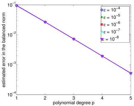
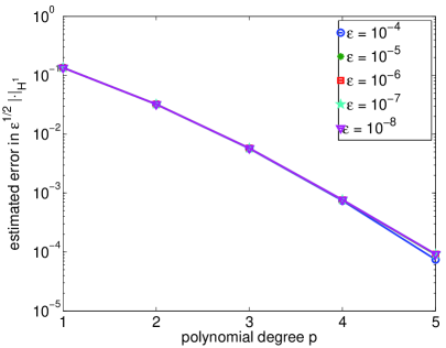
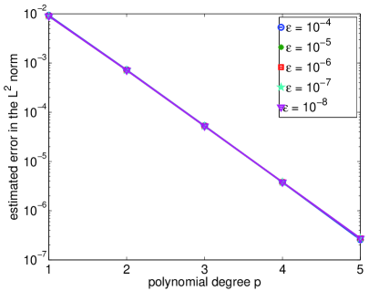
Figure 1: Convergence on Spectral Boundary Layer meshes. Top: convergence in the balanced norm. Bottom left: error $\varepsilon^{1/2}\|(u-u_{FEM})^{\prime}\|_{0,I}$ versus $p$. Bottom right: convergence in $L^{2}$.

3 The two-dimensional case

The ideas of the previous section carry over to the two-dimensional case. We consider the following boundary value problem: Find $u$ such that

$$-\varepsilon^{2}\Delta u+bu = f\quad\text{ in }\Omega\subset\mathbb{R}^{2},$$ (3.1a)

$$u = 0\quad\text{ on }\partial\Omega,$$ (3.1b)

where $\varepsilon\in(0,1]$, and the functions $b$, $f$ are given with $b>0$ on $\overline{\Omega}$. We assume that the data of the problem is analytic, i.e., $\partial\Omega$ is an analytic curve and that there exist constants $C_{f}$, $\gamma_{f}$, $C_{b}$, $\gamma_{b}$, $c_{b}>0$ such that

$$\left\{\begin{array}[]{c}\left\|\nabla^{n}f\right\|_{\infty,\Omega}\leq C_{f}\gamma_{f}^{n}n!\quad\forall\;n\in\mathbb{N}_{0},\\ \left\|\nabla^{n}b\right\|_{\infty,\Omega}\leq C_{b}\gamma_{b}^{n}n!\quad\forall\;n\in\mathbb{N}_{0},\\ \inf_{x\in\Omega}b(x)\geq c_{b}>0.\end{array}\right.$$ (3.2)

The variational formulation of (3.1a), (3.1b) reads: Find $u\in H_{0}^{1}\left(\Omega\right)$ such that

$${\mathcal{B}}_{\varepsilon}(u,v):=\varepsilon^{2}\left\langle\nabla u,\nabla v\right\rangle_{\Omega}+\left\langle bu,v\right\rangle_{\Omega}=F(v):=\left\langle f,v\right\rangle_{\Omega}\quad\forall v\in H_{0}^{1}\left(\Omega\right),$$ (3.3)

where $\left\langle{\cdot,\cdot}\right\rangle_{\Omega}$ denotes the usual $L^{2}(\Omega)$ inner product. As in 1D, the energy norm $\|\cdot\|_{E,\Omega}$ and the balanced norm $\|\cdot\|_{balanced,\Omega}$ are defined by

$$\|v\|^{2}_{E,\Omega} := {\mathcal{B}}_{\varepsilon}(v,v),$$ (3.4)

$$\|v\|^{2}_{balanced,\Omega} := \|v\|^{2}_{0,\Omega}+\varepsilon\|\nabla v\|^{2}_{0,\Omega}$$ (3.5)

The discrete version of (3.3) reads: find $u_{FEM}\in V_{N}\subset H_{0}^{1}\left(\Omega\right)$ such that (3.3) holds for all $v\in V_{N}\subset H_{0}^{1}\left(\Omega\right)$, with $u$ replaced by $u_{FEM}$, where the subspace $V_{N}$ will be defined shortly.

3.1 Meshes and spaces

Concerning the meshes and the $hp$-FEM space based on these meshes, we adopt the simplest case that generalizes our 1D analysis to 2D: The elements are (curvilinear) quadrilaterals and the needle elements required to resolve the boundary layer are obtained as mappings of needle elements of a reference configuration. This approach is discussed in more detail in [7, Sec. 3.1.2] and expanded as the notion of “patchwise structured meshes” in [4, Sec. 3.3.2].

Our $hp$-FEM spaces have the following general structure: Let $\Delta=\left\{\Omega_{i}\right\}_{i=1}^{N}$ be a mesh consisting of curvilinear quadrilaterals $\Omega_{i}$, $i=1,\ldots,N$, subject to the usual restrictions (see, e.g., [7]) and associate with each $\Omega_{i}$ a bijective, Lipschitz continuous (further smoothness assumptions are imposed below) element mapping $M_{i}:S_{ST}\rightarrow\overline{\Omega}_{i},$ where $S_{ST}=[0,1]^{2}$ denotes the usual reference square. With $Q_{p}(S_{ST})$ the space of polynomials of degree $p$ (in each variable) on $S_{ST}$, we set

$$\mathcal{S}^{p}(\Delta) = \left\{u\in H^{1}\left(\Omega\right):\left.u\right|_{\Omega_{i}}\circ M_{i}\in Q_{p}(S_{ST}),\quad i=1,...,N\right\},$$

$$\mathcal{S}_{0}^{p}(\Delta) = \mathcal{S}^{p}(\Delta)\cap H_{0}^{1}(\Omega).$$

We now describe the mesh $\Delta$ and the element maps that we will use (see Fig. 2). Our starting point is a fixed mesh $\Delta_{A}$ (the subscript “$A$” stands for “asymptotic”) consisting of curvilinear quadrilateral elements $\Omega_{i}$, $i=1,\ldots,N^{\prime}$. These elements $\Omega_{i}$ are the images of the reference square $S_{ST}=[0,1]^{2}$ under the element maps $M_{A,i}$, $i=1,\ldots,N^{\prime}$ (we added the subscript “$A$” to emphasize that they correspond to the asymptotic mesh $\Delta_{A}$). They are assumed to satisfy the conditions (M1)–(M3) of [7] in order to ensure that the space ${\mathcal{S}}^{p}(\Delta_{A})$ has suitable approximation properties. The element maps $M_{A,i}$ are assumed to be analytic with analytic inverse; that is, as in [7] we require for some constants $C_{1}$, $C_{2}$, $\gamma>0$

$$\|(M_{A,i}^{\prime})^{-1}\|_{\infty,S_{ST}}\leq C_{1},\qquad\|D^{\alpha}M_{A,i}\|_{\infty,S_{ST}}\leq C_{2}\alpha!\gamma^{|\alpha|}\qquad\forall\alpha\in\mathbb{N}_{0}^{2},\quad i=1,\ldots,N^{\prime}.$$

We furthermore assume that elements do not have a single vertex on the boundary $\partial\Omega$ but only complete, single edges, i.e., the following dichotomy holds:

$$\mbox{ either }\quad\overline{\Omega_{i}}\cap\partial\Omega=\emptyset\quad\mbox{ or }\overline{\Omega_{i}}\cap\partial\Omega\quad\mbox{ is a single edge of $\Omega_{i}$}.$$ (3.6)

Edges of curvilinear quadrilaterals are, of course, the images of the edges of $S_{ST}$ under the element maps. For notational convenience, we assume that the edges lying on $\partial\Omega$ are the image of the edge $\{0\}\times[0,1]$ under the element map. It then follows that these elements have one edge on $\partial\Omega$ and the images of the edges $\{y=1\}$ and $\{y=0\}$ of $S_{ST}$ are shared with elements that likewise have one edge on $\partial\Omega$. For notational convenience, we assume that the elements at the boundary are numbered first, i.e., they are the elements $\Omega_{i}$, $i=1,\ldots,n<N^{\prime}$. For a parameter $\lambda>0$ and a degree $p\in\mathbb{N}$, the boundary layer mesh $\Delta_{BL}=\Delta_{BL}(\lambda,p)$ is defined as follows.

Definition 3.1 (Spectral Boundary Layer mesh $\Delta_{BL}(\lambda,p)$).

Given parameters $\lambda>0$, $p\in\mathbb{N}$, $\varepsilon\in(0,1]$ and the asymptotic mesh $\Delta_{A}$, the mesh $\Delta_{BL}(\lambda,p)$ is defined as follows:

1. $\lambda p\varepsilon\geq 1/2.$ In this case we are in the asymptotic regime, and we use the asymptotic mesh $\Delta_{A}$.

2. $\lambda p\varepsilon<1/2.$ In this regime, we need to define so-called needle elements. This is done by splitting the elements $\Omega_{i},i=1,\ldots,n$ into two elements $\Omega_{i}^{need}$ and $\Omega_{i}^{reg}.$ To that end, split the reference square $S_{ST}$ into two elements

   $$S^{need}=\left[0,\lambda p\varepsilon\right]\times[0,1],\qquad S^{reg}=\left[\lambda p\varepsilon,1\right]\times[0,1],$$

   and define the elements $\Omega_{i}^{need}$, $\Omega_{i}^{reg}$ as the images of these two elements under the element map $M_{A,i}$ and the corresponding element maps as the concatination of the affine maps

   $$A^{need}:S_{ST}\rightarrow S^{need},\qquad(\xi,\eta)\rightarrow(\lambda p\varepsilon\xi,\eta),$$

   $$A^{reg}:S_{ST}\rightarrow S^{reg},\qquad(\xi,\eta)\rightarrow(\lambda p\varepsilon+(1-\lambda p\varepsilon)\xi,\eta)$$

   with the element map $M_{A,i}$, i.e., $M_{i}^{need}=M_{A,i}\circ A^{need}$ and $M_{i}^{reg}=M_{A,i}\circ A^{reg}$. Explicitly:

   $$\Omega_{i}^{need} =M_{A,i}\left(S^{need}\right), \Omega_{i}^{reg} =M_{A,i}\left(S^{reg}\right),$$

   $$M_{i}^{need}(\xi,\eta) =M_{A,i}\left(\lambda p\varepsilon\xi,\eta\right), M_{i}^{reg}(\xi,\eta) =M_{A,i}\left(\lambda p\varepsilon+(1-\lambda p\varepsilon)\xi,\eta\right).$$

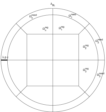
Figure 2: Example of an admissible mesh. Left: asymptotic mesh $\Delta_{A}$. Right: boundary layer mesh $\Delta_{BL}$.

In Figure 2 we show an example of such a mesh construction on the unit circle. In total, the mesh $\Delta_{BL}(\lambda,p)$ consists of $N=N^{\prime}+n$ elements if $\lambda p\varepsilon<1/2$.

Anticipating that we will need, for the case $\lambda p\varepsilon<1/2$, a decomposition of

$$S(\lambda,p):={\mathcal{S}}^{p}(\Delta_{BL}(\lambda,p))$$

into two spaces reflecting the two scales present, we proceed as follows: With $\Delta_{A}$ the asymptotic (coarse) mesh that resolves the geometry we set

$$S_{1} := \mathcal{S}^{p}(\Delta_{A}),$$ (3.7)

$$S_{\varepsilon} := \{v\in{\mathcal{S}}^{p}(\Delta_{BL}(\lambda,p))\,|\,\operatorname*{supp}v\subset\overline{\Omega}_{\lambda p\varepsilon}\},$$ (3.8)

where the boundary layer region $\Omega_{\lambda p\varepsilon}$ is defined as

$$\Omega_{\lambda p\varepsilon}=\overset{n}{\underset{i=1}{\cup}}\Omega_{i}^{need}.$$ (3.9)

As in the 1D situation, our approximation space ${\mathcal{S}}^{p}(\Delta_{BL}(\lambda,p))$ can be written as a direct sum of $S_{1}$ and $S_{\varepsilon}$ if $\lambda p\varepsilon<1/2$:

Lemma 3.2.

Let $\lambda p\varepsilon<1/2$. Then ${\mathcal{S}}^{p}(\Delta_{BL}(\lambda,p))$ is the direct sum $S_{1}\oplus S_{\varepsilon}$. Furthermore, we have the inverse estimates

$$\|u\|_{0,\partial\Omega_{i}} \leq Cp\|u\|_{0,\Omega_{i}}\quad\forall u\in S_{1},\quad i=1,...,N^{\prime},$$ (3.10)

$$|u|_{1,\Omega_{i}} \leq Cp^{2}\|u\|_{0,\Omega_{i}}\quad\forall u\in S_{1},\quad i=1,...,N^{\prime},$$ (3.11)

$$|u|_{1,\Omega_{i}} \leq C\frac{p^{2}}{\lambda p\varepsilon}\|u\|_{0,\Omega_{i}}\quad\forall u\in S_{\varepsilon},i=1,...,n,$$ (3.12)

Proof.

The claim that ${\mathcal{S}}^{p}(\Delta_{BL}(\lambda,p))=S_{1}\oplus S_{\varepsilon}$ follows from the way $\Delta_{BL}(\lambda,p)$ is constructed. Let $z\in{\mathcal{S}}^{p}(\Delta_{BL}(\lambda,p))$. Define $z_{1}\in S_{1}$ as follows: For the internal elements $\Omega_{i}$ with $i=n+1,\ldots,N^{\prime}$ take $z_{1}|_{\Omega_{i}}:=z|_{\Omega_{i}}$. For $\Omega_{i}$, $i\in\{1,\ldots,n\}$, which is further decomposed into $\Omega_{i}^{need}$ and $\Omega_{i}^{reg}$, we consider the pull-back $\widetilde{z}_{i}:=z|_{\Omega_{i}}\circ M_{A,i}$. This pull-back $\widetilde{z}_{i}$ is a piecewise polynomial on $S_{ST}=S^{need}\cup S^{reg}$. Define the polynomial $\widehat{z}_{i}\in Q(S_{ST})$ on the full reference element $S_{ST}$ by the condition

$$\widehat{z}_{i}|_{S^{reg}}=\widetilde{z}_{i}|_{S^{reg}}$$

and then set $z_{1}|_{\Omega_{i}}:=\widehat{z}_{i}\circ M_{A,i}^{-1}$; that is, the restriction $\widetilde{z}_{i}|_{S^{reg}}$ is extended polynomially to $S_{ST}$. In this way, the function $z_{1}$ is defined elementwise, and the assumptions on the element maps $M_{A,i}$ of the asymptotic mesh $\Delta_{A}$ ensure that $z_{1}\in H^{1}(\Omega)$, i.e., $z_{1}\in S_{1}$. Since by construction $z|_{\Omega_{i}^{reg}}=z_{1}|_{\Omega_{i}^{reg}}$ for $i=1,\ldots,n$, we conclude that $\operatorname*{supp}(z-z_{1})\subset\overline{\Omega}_{\lambda p\varepsilon}$ and therefore $z_{\varepsilon}:=z-z_{1}\in S_{\varepsilon}$. The construction also shows the uniqueness of the decomposition.

The inverse estimates (3.10), (3.11), (3.12) can be seen as follows. The estimate (3.11) is an easy consequence of the assumptions on the element maps $M_{A,i}$ of the asymptotic mesh $\Delta_{A}$ and the polynomial inverse estimates [12, Thm. 4.76]. In a similar manner, the inverse estimate (3.10), which estimates the $L^{2}$-norm on the boundary $\partial\Omega_{i}$ of $\Omega_{i}$ by the $L^{2}$-norm on $\Omega_{i}$ follows from a suitable application of 1D inverse estimates (cf. [12, eqn. (3.6.4)]).

For the estimate (3.12), we note that for an element $\Omega_{i}^{need}$, we can estimate for any $v\in S_{\varepsilon}$ again with assumptions on the element maps $M_{A,i}$

$$\|\nabla v\|_{0,\Omega_{i}^{need}}\sim\|\nabla(v\circ M_{A,i})\|_{0,S^{need}}\leq C\frac{p^{2}}{\lambda p\varepsilon}\|v\circ M_{A,i}\|_{0,S^{need}}\sim C\frac{p^{2}}{\lambda p\varepsilon}\|v\|_{0,S^{need}},$$

where we exploited that $v\circ M_{A,i}$ is a polynomial of degree $p$ and used the inverse estimate [12, Thm. 3.91]. ∎

We mention already at this point that we will quantify the contributions $z_{1}$ and $z_{\varepsilon}$ of this decomposition in Lemma 3.9 ahead. We close this section by pointing out that in our setting, one has very good control over the element maps: There exist $C>0$ (depending solely on the asymptotic mesh $\Delta_{A}$) such that

$$\|M^{\prime}_{A,i}\|_{\infty,S_{ST}}+\|(M^{\prime}_{A,i})^{-1}\|_{\infty,S_{ST}} \leq C,\quad i=1,\ldots,N^{\prime},$$ (3.13a)

$$\|(M^{reg}_{i})^{\prime}\|_{\infty,S_{ST}}+\|((M^{reg}_{i})^{\prime})^{-1}\|_{\infty,S_{ST}} \leq C,\quad i=1,\ldots,n,$$ (3.13b)

$$\|(M^{need}_{i})^{\prime}\|_{\infty,S_{ST}}+\|((M^{need}_{i})^{\prime})^{-1}\|_{\infty,S_{ST}} \leq C\frac{1}{\lambda p\varepsilon},\quad i=1,\ldots,n.$$ (3.13c)

3.2 Approximation properties of the Spectral Boundary Layer mesh

By construction, the resulting mesh (in the case $\lambda p\varepsilon<1/2$)

$$\Delta_{BL}=\Delta_{BL}(\lambda,p)=\left\{\Omega_{1}^{need},...,\Omega_{n}^{need},\Omega_{1}^{reg},...,\Omega_{n}^{reg},\Omega_{n+1},...,\Omega_{N}\right\}$$

is a regular admissible mesh in the sense of [7]. Therefore, [7] gives that the space

$$S_{0}(\lambda,p):={\mathcal{S}}^{p}_{0}(\Delta_{BL}(\lambda,p))$$

has the following approximation properties:

Proposition 3.3 ([7]).

Let $u$ be the solution to (3.3) and assume that (3.2) holds. Then there exist constants $\lambda_{0}$, $\lambda_{1}$, $C$, $\beta>0$ independent of $\varepsilon\in(0,1]$ and $p\in\mathbb{N}$, such that the following is true: For every $p$ and every $\lambda\in(0,\lambda_{0}]$ with $\lambda p\geq\lambda_{1}$ there exists $\pi_{p}u\in\mathcal{S}_{0}^{{p}}(\Delta_{BL}(\lambda,p))$ such that

$$\left\|u-\pi_{p}u\right\|_{\infty,\Omega}+\varepsilon\left\|\nabla(u-\pi_{p}u)\right\|_{\infty,\Omega}\leq Cp^{2}\left(\ln p+1\right)^{2}e^{-\beta p\lambda}.$$

We mention in passing that Proposition 3.3 provides robust exponential convergence in the energy norm. However, as in the 1D case of Lemma 2.5, we can modify the boundary layer part of the approximant of Proposition 3.3, so as to be able to approximate at a robust exponential rate in the balanced norm. This is achieved with the following 2D analog of Lemma 2.4.

Lemma 3.4.

Let $v$ be defined on $S=[0,1]^{2}$, and let $v$ be analytic on $[0,d_{0}]\times[0,1]$ for some fixed $d_{0}\in(0,1]$. Assume that for some $C_{v}$, $\gamma_{v}>0$ and $\varepsilon\in(0,1]$, the function $v$ satisfies the following hypotheses:

• For every $\xi\in(0,d_{0})$, the stretched function $\widehat{v}_{\xi}:S\rightarrow\mathbb{R}$ given by $\widehat{v}_{\xi}(x,y):=u(x\xi,y)$, satisfies

  $$\|D^{\alpha}\widehat{v}_{\xi}\|_{\infty,S}\leq C_{v}\gamma_{v}^{|\alpha|}\max\{|\alpha|+1,\xi/\varepsilon\}^{|\alpha|}\qquad\forall\alpha\in\mathbb{N}_{0}^{2}.$$

• The function $v$ satisfies

  $$\sup_{y\in[0,1]}|\nabla^{n}v(x,y)|\leq C_{v}\varepsilon^{-n}e^{-x/\varepsilon}\qquad\forall x\in[0,1],\quad n\in\{0,1\}.$$

Then there are constants $C$, $\beta$, $\eta>0$ (depending only on $\gamma_{v}$) such that under the assumption

$$\frac{\xi}{p\varepsilon}\leq\eta,$$

the following is true for the mesh $\Delta_{\xi}=\{S_{\xi}^{need},S_{\xi}^{reg}\}$ with $S_{\xi}^{need}:=[0,\xi]\times[0,1]$ and $S_{\xi}^{reg}:=[\xi,1]\times[0,1]$: There there is a piecewise polynomial approximation $I_{p}v\in{\mathcal{S}}^{p}(\Delta_{\xi})$ with the following properties:

1. On the two edges $x=0$ and $x=1$ of $S$, the approximation $I_{p}v$ coincides with the Gauß-Lobatto interpolant of $v$. On the edge $(0,\xi)\times\{0\}$, $I_{p}v$ is given by the Gauß-Lobatto interpolant corrected by $(1-\sqrt{\varepsilon})\frac{x}{\xi}v(\xi,0)$ (so that $(I_{p}v)(\xi,0)=\sqrt{\epsilon}v(\xi,0)$), and on the edge $(\xi,1)\times\{0\}$, $I_{p}v$ is the linear polynomial interpolating the values $\sqrt{\varepsilon}v(\xi,0)$ and $v(1,0)$ at the endpoints. $I_{p}v$ is defined analogously on the edges $(0,\xi)\times\{1\}$ and $(\xi,1)\times\{1\}$.

2. The approximation $I_{p}v$ satisfies

   $$\|(v-I_{p}v)\|_{\infty,S_{\xi}^{need}}+\xi\|\partial_{x}(v-I_{p}v)\|_{\infty,S_{\xi}^{need}}+\|\partial_{y}(v-I_{p}v)\|_{\infty,S_{\xi}^{need}}$$

   $$\leq CC_{v}\left[e^{-\beta p}+p^{2}(1+\ln p)^{2}e^{-\xi/\varepsilon}\right],$$

   $$\|v-I_{p}v\|_{\infty,S_{\xi}^{reg}}\leq CC_{v}(1+\ln p)^{2}e^{-\xi/\varepsilon},$$

   $$\|v-I_{p}v\|_{0,S_{\xi}^{reg}}+\varepsilon\|\nabla(v-I_{p}v)\|_{0,S_{\xi}^{reg}}\leq CC_{v}p^{2}(1+\ln p)^{2}\sqrt{\varepsilon}e^{-\xi/\varepsilon}.$$

Proof.

As in the corresponding 1D result (Lemma 2.4), we construct $I_{p}v$ in two steps. In the first step, we study the approximation $v_{1}$ which is given by the piecewise Gauß-Lobatto interpolant. In the second step, we modify $v_{1}$ to obtain the additional factor $\sqrt{\varepsilon}$ for the error in the $L^{2}$-based norms on the large element $S_{\xi}^{reg}$.

Step 1: For $\xi\in(0,d_{0})$, let $v_{1}$ be the piecewise Gauß-Lobatto interpolant of $v$ on the mesh $\Delta_{\xi}$. For simplicity, we assume $\xi\leq 1/2$. The error analysis for $v-v_{1}$ can be extracted from the proof of [7, Thm. 3.12]; we highlight here the main arguments for completeness’ sake. The one-dimensional Gauß-Lobatto interpolation operator $i_{p}:C([0,1])\rightarrow\Pi_{p}$ has the stability property $\|i_{p}\|_{\infty,[0,1]}\leq C(1+\ln p)$ by [15]. Together with a polynomial inverse estimate (Markov’s inequality) we get on $S_{\xi}^{reg}$:

$$\|v_{1}\|_{\infty,S_{\xi}^{reg}} \leq C(1+\ln p)^{2}\|v\|_{\infty,S_{\xi}^{reg}}\leq CC_{v}(1+\ln p)^{2}e^{-\xi/\varepsilon},$$

$$\|\nabla v_{1}\|_{\infty,S_{\xi}^{reg}} \leq Cp^{2}\|v_{1}\|_{\infty,S_{\xi}^{reg}}\leq Cp^{2}(1+\ln p)^{2}\|v\|_{\infty,S_{\xi}^{reg}}\leq CC_{v}p^{2}(1+\ln p)^{2}e^{-\xi/\varepsilon}.$$

The error analysis for the Gauß-Lobatto interpolation on $S_{\xi}^{need}$ is achieved by (anisotropically) scaling $S_{\xi}^{need}$ to the reference element $S=[0,1]^{2}$. In order to make use of the regularity properties of the scaled function $\widehat{v}$, we first observe that for $n\in\mathbb{N}_{0}$

$$\max\{n+1,\xi/\varepsilon\}^{n} =\max\{(n+1)^{n},\frac{1}{n!}(\xi/\varepsilon)^{n}n!\}\leq\max\{(n+1)^{n},n!e^{\xi/\varepsilon}\}\leq n!e^{\xi/\varepsilon}\frac{(n+1)^{n}}{n!}$$

$$\leq Cn!e^{n}e^{\xi/\varepsilon},$$

for some $C>0$, where the last inequality follows from Stirling’s formula. The tensor product Gauß-Lobatto interpolant $\widehat{v}_{1}$ of the stretched function $\widehat{v}_{\xi}$ satisfies on $S$

$$\|\widehat{v}_{\xi}-\widehat{v}_{1}\|_{\infty,S}+\|\nabla(\widehat{v}_{\xi}-\widehat{v}_{1})\|_{\infty,S}\leq CC_{v}e^{\xi/\varepsilon}e^{-\beta p},$$

for some $C$, $\beta>0$ that depend solely on $\gamma_{v}$. Returning to $S_{\xi}^{need}$, we get for the Gauß-Lobatto interpolation error

$$\|v-v_{1}\|_{\infty,S_{\xi}^{need}}+\xi\|\partial_{x}(v-v_{1})\|_{\infty,S_{\xi}^{need}}+\|\partial_{y}(v-v_{1})\|_{\infty,S_{\xi}^{need}}\leq CC_{v}e^{\xi/\varepsilon}e^{-\beta p}.$$

Step 2: We define $I_{p}v$ as follows (thus correcting $v_{1}$):

$$I_{p}v(x,y):=\begin{cases}v_{1}(x,y)-(1-\sqrt{\varepsilon})v_{1}(\xi,y)\frac{x}{\xi},&(x,y)\in S_{\xi}^{need}\\ \sqrt{\varepsilon}v_{1}(\xi,y)\frac{1-x}{1-\xi}+\frac{x-\xi}{1-\xi}v_{1}(1,y),&(x,y)\in S_{\xi}^{reg}.\end{cases}$$

We note

$$\sup_{y\in[0,1]}|v_{1}(\xi,y)|\leq CC_{v}(1+\ln p)^{2}e^{-\xi/\varepsilon},\qquad\sup_{y\in[0,1]}|\partial_{y}v_{1}(\xi,y)|\leq CC_{v}p^{2}(1+\ln p)^{2}e^{-\xi/\varepsilon},$$

$$\sup_{y\in[0,1]}|v_{1}(1,y)|\leq CC_{v}(1+\ln p)^{2}e^{-1/\varepsilon},\qquad\sup_{y\in[0,1]}|\partial_{y}v_{1}(1,y)|\leq CC_{v}p^{2}(1+\ln p)^{2}e^{-1/\varepsilon}.$$

From this, we get on $S_{\xi}^{need}$

$$\|v-I_{p}v\|_{\infty,S_{\xi}^{need}}+\xi\|\partial_{x}(v-I_{p}v)\|_{\infty,S_{\xi}^{need}}+\|\partial_{y}(v-I_{p}v)\|_{\infty,S_{\xi}^{need}}$$

$$\leq CC_{v}\left[e^{\xi/\varepsilon}e^{-\beta p}+p^{2}(1+\ln p)^{2}e^{-\xi/\varepsilon}\right].$$

The hypothesis $\xi/\varepsilon\leq\eta p$ implies that $e^{\xi/\varepsilon}e^{-\beta p}\leq e^{(\eta-\beta)p}$, so that $\eta<\beta$ guarantees exponential convergence (in $p$). The claimed approximation properties on $S_{\xi}^{need}$ follow.

The approximations on $S_{\xi}^{reg}$ are achieved by the triangle inequality $\|v-I_{p}v\|\leq\|v\|+\|I_{p}v\|$. The control of $I_{p}v$ is easily achieved by observing

$$\|I_{p}v\|_{\infty,S_{\xi}^{reg}}\leq CC_{v}(1+\ln p)^{2}\sqrt{\varepsilon}e^{-\xi/\varepsilon}\;,\;\|\nabla I_{p}v\|_{\infty,S_{\xi}^{reg}}\leq CC_{v}p^{2}(1+\ln p)^{2}\sqrt{\varepsilon}e^{-\xi/\varepsilon}.$$

Note that we suppressed the contributions arising from $v_{1}(1,\cdot)$ since our assumption $\xi\leq 1/2$ provides $e^{-1/\varepsilon}\leq C\sqrt{\varepsilon}e^{-\xi/\varepsilon}$ for some $C>0$. ∎

The improved treatment of the boundary layer contribution allows us to sharpen the approximation result of Proposition 3.3 in the balanced norm:

Corollary 3.5.

Under the assumptions of Proposition 3.3, there exist constants $\lambda_{0}$, $\lambda_{1}$, $C$, $\beta>0$ independent of $\varepsilon\in(0,1]$ and $p\in\mathbb{N}$, such that the following is true: For every $p$ and every $\lambda\in(0,\lambda_{0}]$ with $\lambda p\geq\lambda_{1}$, there exists $\widetilde{\pi}_{p}u\in\mathcal{S}_{0}^{{p}}(\Delta_{BL}(\lambda,p))$ such that

$$\|u-\widetilde{\pi}_{p}u\|_{\infty,\Omega}+\varepsilon^{1/2}\left\|\nabla(u-\widetilde{\pi}_{p}u)\right\|_{0,\Omega}\leq Cp^{2}\left(\ln p+1\right)^{2}e^{-\beta p\lambda}.$$

Proof.

In the case that the mesh $\Delta_{BL}(\lambda,p)$ consists of the asymptotic mesh $\Delta_{A}$, we set $\widetilde{\pi}_{p}u=\pi_{p}u$ and the proof follows easily from Proposition 3.3, since $\varepsilon\geq 1/(2\lambda p)\geq 1/(2\lambda_{1})$. Let, therefore, $\Delta_{BL}(\lambda,p)$ have needle elements, i.e., the elements $\Omega_{i}$, $i=1,\ldots,n$ of the asymptotic mesh $\Delta_{A}$ are further subdivided into $\Omega_{i}^{need}$ and $\Omega_{i}^{reg}$. Our starting point is the proof of Proposition 3.3 in [7]. There, the approximation is obtained by a piecewise Gauß-Lobatto interpolation of the function $u$, which is decomposed into a smooth (analytic) part $w$, a boundary layer part $u^{BL}$, and a remainder $r$:

$$u=w+u^{BL}+r.$$

The approximations of the smooth part $w$ and the remainder $r$ are taken to be those of [7], i.e., the elementwise Gauß-Lobatto interpolants. The boundary layer part $u^{BL}$, however, is not approximated by its elementwise Gauß-Lobatto interpolant but by the elementwise Gauß-Lobatto interpolant on the elements $\Omega_{i}$ with $\overline{\Omega_{i}}\cap\partial\Omega=\emptyset$, with the aid of the operator $I_{p}$ of Lemma 3.4. Inspection of the procedure in [7] shows that the regularity hypotheses (R1), (R2) of Lemma 3.4 are satisfied and that the approximation result holds if $\xi=\lambda p\varepsilon$ with $\lambda\leq\lambda_{0}$ and $\lambda_{0}$ sufficiently small. ∎

3.3 Robust exponential convergence in balanced norms

The main result of the paper is the following robust exponential convergence in the balanced norm:

Theorem 3.6.

There is a $\lambda_{0}>0$ depending only on the functions $b$, $f$ and the asymptotic mesh $\Delta_{A}$ such that for every $\lambda\in(0,\lambda_{0}]$, $\varepsilon\in(0,1]$, $p\in\mathbb{N}$, the $hp$-FEM space $\mathcal{S}_{0}^{p}(\Delta_{BL}(\lambda,p))$ leads to a finite element approximation $u_{FEM}\in\mathcal{S}_{0}^{p}(\Delta_{BL}(\lambda,p))$ satisfying

$$\sqrt{\varepsilon}\|\nabla(u-u_{FEM})\|_{0,\Omega}+\|u-u_{FEM}\|_{0,\Omega}\leq Ce^{-\beta p};$$

the constants $C$, $\beta>0$ depend on the choice of $\lambda$ but are independent of $\varepsilon$ and $p$.

The proof is deferred to the end of the section. As a corollary, we get exponential convergenence in the maximum norm.

Corollary 3.7.

Let $u$ be the solution of (3.3) and let $u_{FEM}\in{\mathcal{S}}_{0}^{p}(\Delta_{BL}(\lambda,p))$ be its finite element approximation. Then there exist constants $C$, $\sigma>0$ independent of $\varepsilon\in(0,1]$ and $p\in\mathbb{N}$ such that

$$\left\|u-u_{FEM}\right\|_{\infty,\Omega}\leq Ce^{-\sigma p}.$$

Proof.

First we note that Corollary 3.5 provides an approximation $\pi_{p}u\in{\mathcal{S}}_{0}^{p}(\Delta_{BL}(\lambda,p))$ with

$$\left\|u-\pi_{p}u\right\|_{\infty,\Omega}\leq Ce^{-\beta\lambda p}.$$

In view of the triangle inequality $\displaystyle\left\|u-u_{FEM}\right\|_{\infty,\Omega}\leq\left\|u-\pi_{p}u\right\|_{\infty,\Omega}+\left\|\pi_{p}u-u_{FEM}\right\|_{\infty,\Omega},$ we may focus on the term $\left\|\pi_{p}u-u_{FEM}\right\|_{\infty,\Omega}$. It suffices to prove the result in the layer region, i.e., for the elements $\Omega_{i}^{need}$, since outside $\Omega_{\lambda p\varepsilon}$ standard inverse estimates (bounding the $L^{\infty}$-norm of polynomials by their $L^{2}$-norm up to powers of $p$) yield the desired bound in view of (3.13a), (3.13b).

For a needle element $\Omega_{i}^{need}$ we introduce $\widetilde{\pi}_{p}u:=\pi_{p}u|_{\Omega_{i}^{need}}\circ M_{A,i}$ and $\widetilde{u}_{FEM}:=u_{FEM}|_{\Omega_{i}^{need}}\circ M_{A,i}$. The polynomial inverse estimate of [12, Thm. 4.76] and an affine scaling argument (between $S_{ST}$ and $S^{need}$) yield

$$\left\|\pi_{p}u-u_{FEM}\right\|_{\infty,\Omega_{i}^{need}} =\left\|\widetilde{\pi}_{p}u-\widetilde{u}_{FEM}\right\|_{\infty,S^{need}}\leq C\frac{p^{2}}{\sqrt{\lambda p\varepsilon}}\left\|\widetilde{\pi}_{p}u-\widetilde{u}_{FEM}\right\|_{0,S^{need}}$$

$$\sim\frac{p^{2}}{\sqrt{\lambda p\varepsilon}}\left\|\pi_{p}u-u_{FEM}\right\|_{0,\Omega_{i}^{need}},$$

where in the last step we used the assumptions on the element maps $M_{A,i}$. The triangle inequality then gives

$$\left\|\pi_{p}u-u_{FEM}\right\|_{\infty,\Omega_{i}^{need}}\leq C\frac{p^{2}}{\sqrt{\lambda p\varepsilon}}\left[\left\|\pi_{p}u-u\right\|_{0,\Omega_{i}^{need}}+\left\|u-u_{FEM}\right\|_{0,\Omega_{i}^{need}}\right].$$ (3.14)

For the first term in (3.14) we obtain from the $L^{\infty}$-bound of Corollary 3.5 and the fact that $|\Omega_{i}^{need}|\sim\lambda p\varepsilon$,

$$\left\|\pi_{p}u-u\right\|_{0,\Omega_{i}^{need}}\lesssim\sqrt{\lambda p\varepsilon}e^{-\beta p}.$$ (3.15)

For the second term in (3.14) we exploit the fact that $u_{FEM}=0=\pi_{p}u$ on $\partial\Omega$ and a 1D Poincaré inequality. To that end, we note that for any function $\widetilde{v}\in H^{1}(S^{need})$ with $v=0$ on the edge $\{(0,y)\,|\,0\leq y\leq 1\}$ of $S^{need}=\{(x,y)\,|\,0\leq x\leq\lambda p\varepsilon,0\leq y\leq 1\}$, we obtain from a 1D Poincaré inequality

$$\|\widetilde{v}\|_{0,S^{need}}\leq C\sqrt{\lambda p\varepsilon}\|\partial_{x}\widetilde{v}\|_{0,S^{need}}\leq C\sqrt{\lambda p\varepsilon}\|\nabla\widetilde{v}\|_{0,S^{need}}.$$ (3.16)

Upon setting $\widetilde{v}:=(u-u_{FEM})|_{\Omega_{i}^{need}}\circ M_{A,i}$, we may use (3.16) together with the properties of $M_{A,i}$ to get

$$\|u-u_{FEM}\|_{0,\Omega_{i}^{need}}\sim\|\widetilde{v}\|_{0,S^{need}}\leq C\sqrt{\lambda p\varepsilon}\|\nabla\widetilde{v}\|_{0,S^{need}}\sim\sqrt{\lambda p\varepsilon}\|\nabla(u-u_{FEM})\|_{0,\Omega_{i}^{need}}.$$ (3.17)

Combining (3.14), (3.15), (3.17) gives the desired result. ∎

3.4 Proof of Theorem 3.6

The proof of Theorem 3.6 parallels that of the 1D case in Section 2. We begin by defining the bilinear form for the reduced problem,

$${\mathcal{B}}_{0}(u,v)=\left\langle bu,v\right\rangle_{\Omega}.$$ (3.18)

We also introduce the projection operator $\mathcal{P}_{0}:L^{2}(\Omega)\rightarrow\mathcal{S}_{0}^{p}(\Delta_{BL}(\lambda,p))$ by the condition

$${\mathcal{B}}_{0}\left(u-\mathcal{P}_{0}u,v\right)=0\quad\forall v\in\mathcal{S}_{0}^{p}(\Delta_{BL}(\lambda,p)).$$

Then, by reasoning as in (2.3.1) with Galerkin orthogonalities, we get

$$\left\|u_{FEM}-\mathcal{P}_{0}u\right\|_{E,\Omega}^{2} = \varepsilon^{2}\left\langle\nabla\left(u-\mathcal{P}_{0}u\right),\nabla\left(u_{FEM}-\mathcal{P}_{0}u\right)\right\rangle_{\Omega}.$$

Hence

$$\varepsilon\left\|\nabla\left(u_{FEM}-\mathcal{P}_{0}u\right)\right\|_{0,\Omega}\leq\left\|u_{FEM}-\mathcal{P}_{0}u\right\|_{E,\Omega}\leq\varepsilon\left\|\nabla\left(u-\mathcal{P}_{0}u\right)\right\|_{0,\Omega}.$$

The key step towards showing robust exponential convergence in balanced norms is therefore to show

$$\left\|\nabla\left(u-\mathcal{P}_{0}u\right)\right\|_{0,\Omega}\leq C\varepsilon^{-1/2}e^{-\sigma p},$$

for some $C$ and $\sigma>0$ independent of $\varepsilon$ and $p$. Completely analogous to the one-dimensional case, we are therefore led to studying the $H^{1}$-stability of the projection operator $\mathcal{P}_{0}$ on the Spectral Boundary Layer mesh of Definition 3.1.

Lemma 3.8 (Strengthened Cauchy-Schwarz inequality in 2D).

Let ${\mathcal{B}}_{0}$ be given by (3.18). Then,

$$\left|{\mathcal{B}}_{0}\left(u,v\right)\right|\leq C\min\{1,\sqrt{\lambda p\varepsilon}p\}\left\|u\right\|_{0,\Omega}\left\|v\right\|_{0,\Omega_{\lambda p\varepsilon}}\quad\forall u\in S_{1},\quad v\in S_{\varepsilon},$$

with $S_{1}$, $S_{\varepsilon}$ given by (3.7) and (3.8), respectively. The constant $C>0$ depends solely on $\|b\|_{\infty,\Omega}$, $\inf_{x\in\Omega}b(x)>0$, and the element maps of the asymptotic mesh $\Delta_{A}$.

Proof.

We restrict our attention to the case $\lambda p\varepsilon<1/2$ as the “$1$” in the minimum is a simple consequence of the Cauchy-Schwarz inequality. With $u\in S_{1}$, $v\in S_{\varepsilon}$ there holds ${\mathcal{B}}_{0}(u,v)=\iint_{\Omega_{\lambda p\varepsilon}}buv$. Fix $\Omega_{i}^{need}$ and recall that it is obtained from an element $\Omega_{i}$ ($i\in\{1,\ldots,n\}$) by a splitting, i.e., $\overline{\Omega}_{i}=\overline{\Omega^{need}_{i}}\cup\overline{\Omega^{reg}_{i}}$. The construction of $\Delta_{BL}(\lambda,p)$ implies that the pull-back $\pi_{1}:=u|_{\Omega_{i}}\circ M_{A,i}$ to $S_{ST}$ is a polynomial of degree $p$ (in each variable) whereas the pull-back $\pi_{2}:=v|_{\Omega_{i}}\circ M_{A,i}$ is a piecewise polynomial of degree $p$ (in each variable) with $\operatorname*{supp}\pi_{2}\subset S^{need}$. Upon setting $\widehat{b}:=b|_{\Omega_{i}^{need}}\circ M_{A,i}$, which is uniformly bounded on $S^{need}$, we calculate

$$\iint_{\Omega_{i}}buv\,dx\,dy =\iint_{\Omega_{i}^{need}}buv\,dx\,dy=\iint_{S^{need}}\pi_{1}(x,y)\pi_{2}(x,y)\,\widehat{b}|\operatorname*{det}M_{A,i}^{\prime}|\,dx\,dy.$$

Since $|\operatorname*{det}M_{A,i}^{\prime}|$ is bounded uniformly (in $(x,y)$), we obtain

$$\left|\iint_{\Omega_{i}^{need}}buv\right|\leq C\iint_{S^{need}}|\pi_{1}(x,y)||\pi_{2}(x,y)|dxdy=C\int_{0}^{1}\int_{0}^{\lambda p\varepsilon}|\pi_{1}(x,y)||\pi_{2}(x,y)|dxdy.$$

Now, fix $y\in[0,1]$ and consider

$$\int_{0}^{\lambda p\varepsilon}|\pi_{1}(x,y)||\pi_{2}(x,y)|dx\leq Cp\sqrt{\lambda p\varepsilon}\left[\int_{0}^{1}|\pi_{1}(x,y)|^{2}dx\right]^{1/2}\left[\int_{0}^{\lambda p\varepsilon}|\pi_{2}(x,y)|^{2}dx\right]^{1/2}$$

by Lemma 2.8. Integrating in $y$ from 0 to 1, gives

$$\int_{0}^{1}\int_{0}^{\lambda p\varepsilon}|\pi_{1}(x,y)||\pi_{2}(x,y)|dxdy\leq Cp\sqrt{\lambda p\varepsilon}\int_{0}^{1}\left[\int_{0}^{1}|\pi_{1}(x,y)|^{2}dx\right]^{1/2}\left[\int_{0}^{\lambda p\varepsilon}|\pi_{2}(x,y)|^{2}dx\right]^{1/2}dy.$$

Using once more the Cauchy-Schwarz inequality, we arrive at

$$\iint_{S^{need}}|\pi_{1}(x,y)||\pi_{2}(x,y)|dxdy\leq Cp\sqrt{\lambda p\varepsilon}\|\pi_{1}\|_{0,S_{ST}}\|\pi_{2}\|_{0,S^{need}}.$$

The assumptions on the element map $M_{A,i}$ allows us to infer $\|\pi_{1}\|_{0,S_{ST}}\|\pi_{2}\|_{0,S^{need}}\sim\|u\|_{0,\Omega_{i}}\|v\|_{0,\Omega_{i}^{need}}$, which concludes the proof. ∎

Lemma 3.9 (Stability of ${\mathcal{P}}_{0}$).

There exist constants $C$, $c>0$ depending solely on $\|b\|_{\infty,\Omega}$, $\inf_{x\in\Omega}b(x)>0$, and the element maps of the asymptotic mesh $\Delta_{A}$ such that the following is true under the assumption

$$\sqrt{\lambda p\varepsilon}p\leq c:$$ (3.19)

For each $z\in L^{2}(\Omega)$, the (unique) decomposition

$${\cal{P}}_{0}z=z_{1}+z_{\varepsilon}$$

into the components $z_{1}\in S_{1}$ and $z_{\varepsilon}\in S_{\varepsilon}$ satisfies

$$\|z_{1}\|_{0,\Omega} \leq C\|z\|_{0,\Omega},$$ (3.20)

$$\|z_{\varepsilon}\|_{0,\Omega} \leq C\{\|z\|_{0,\Omega_{\lambda p\varepsilon}}+\sqrt{\lambda p\varepsilon}p\|z\|_{0,\Omega}\}.$$ (3.21)

Furthermore,

$$\|\nabla z_{1}\|_{0,\Omega} \leq Cp^{2}\|z\|_{0,\Omega},$$ (3.22)

$$\|\nabla z_{\varepsilon}\|_{0,\Omega} \leq C\frac{p^{2}}{\lambda p\varepsilon}\left\{\|z\|_{0,\Omega_{\lambda p\varepsilon}}+\sqrt{\lambda p\varepsilon}p\|z\|_{0,\Omega}\right\}.$$ (3.23)

Proof.

The proof parallels that of Lemma 2.9. With Lemma 3.2 we can write ${\mathcal{P}}_{0}z=z_{1}+z_{\varepsilon}$. We define the auxiliary function $\psi_{\varepsilon}$ on $S_{ST}$ by

$$\psi_{\varepsilon}(x,y):=\begin{cases}\left(1-\frac{2x}{\lambda p\varepsilon}\right)^{p}&\text{ if }(x,y)\in S^{need}\\ 0&\text{ otherwise.}\end{cases}$$

Then $\text{supp }\psi_{\varepsilon}\subset S^{need},\psi_{\varepsilon}(0,y)=1$ and $\left\|\psi_{\varepsilon}\right\|_{0,S_{ST}}=\left\|\psi_{\varepsilon}\right\|_{0,S^{need}}\sim p^{-1/2}\sqrt{\lambda p\varepsilon}$. We define the function $\widetilde{z}_{\varepsilon}\in S_{\varepsilon}$ on the needle elements $\Omega_{i}^{need}$ by prescribing its pull-back to $S^{need}$:

$$(\widetilde{z}_{\varepsilon}|_{\Omega_{i}^{need}}\circ M_{A,i})(x,y):=(z_{\varepsilon}|_{\Omega_{i}^{need}}\circ M_{A,i})(x,y)+\psi_{\varepsilon}(x,y)(z_{1}|_{\Omega_{i}}\circ M_{A,i})(0,y),\qquad(x,y)\in S^{need};$$

here, $\Omega_{i}$ and $\Omega_{i}^{need}$ are related to each other by $\Omega_{i}=\Omega_{i}^{need}\cup\Omega_{i}^{reg}$. It is an effect of the assumptions on the asymptotic mesh $\Delta_{A}$ that the elementwise defined function $\widetilde{z}_{\varepsilon}$ is in fact in $H^{1}(\Omega)$ and therefore indeed $z_{\varepsilon}\in S_{\varepsilon}$. By construction, $\widetilde{z}_{\varepsilon}|_{\partial\Omega}=(z_{1}+z_{\varepsilon})|_{\partial\Omega}=({\mathcal{P}}_{0}z)|_{\partial\Omega}=0$ so that $\widetilde{z}_{\varepsilon}\in S_{\varepsilon}\cap S_{0}(\lambda,p)$. Noting the product structure of $(z_{\varepsilon}-\widetilde{z}_{\varepsilon})|_{\Omega_{i}^{need}}\circ M_{A,i}$ on $S^{need}$ and the above estimate on $\|\psi_{\varepsilon}\|_{0,S^{need}}$, we get for $\widetilde{z}_{\varepsilon}$ with the inverse estimate (3.10),

$$\left\|\widetilde{z}_{\varepsilon}\right\|_{0,\Omega}=\left\|\widetilde{z}_{\varepsilon}\right\|_{0,\Omega_{\lambda p\varepsilon}}\leq C\left\{\left\|z_{\varepsilon}\right\|_{0,\Omega_{\lambda\varepsilon}}+p^{1/2}\sqrt{\lambda p\varepsilon}\left\|z_{1}\right\|_{0,\Omega}\right\}.$$

We also have in view of ${\mathcal{P}}_{0}z=z_{1}+z_{\varepsilon}$

$$B_{0}(z_{1},v_{1})+B_{0}(z_{\varepsilon},v_{1}) = B_{0}(\mathcal{P}_{0}z,v_{1})\quad\forall v_{1}\in S_{1},$$ (3.24)

$$B_{0}(z_{1},v_{\varepsilon})+B_{0}(z_{\varepsilon},v_{\varepsilon}) = B_{0}(\mathcal{P}_{0}z,v_{\varepsilon})=B_{0}(z,v_{\varepsilon})\quad\forall v_{\varepsilon}\in{S}_{\varepsilon}\cap\mathcal{S}_{0}^{p}\left(\Delta_{BL}(\lambda,p)\right),$$ (3.25)

where in (3.25) we used the fact that $\mathcal{P}_{0}$ is the ${\mathcal{B}}_{0}$–projection onto $\mathcal{S}_{0}^{p}\left(\Delta_{BL}(\lambda,p)\right)$. Taking $v_{1}=z_{1}$ in (3.24) and $v_{\varepsilon}=\widetilde{z}_{\varepsilon}\in S_{\varepsilon}\cap\mathcal{S}_{0}^{p}\left(\Delta_{BL}(\lambda,p)\right)$ in (3.25) yields, together with the Strengthened Cauchy Schwarz inequality of Lemma 2.9, just like in the 1D case, the bounds (3.20), (3.21). The final estimates (3.22), (3.23) follow from (3.20, (3.21) with the aid of the inverse estimates (3.11), (3.12) of Lemma 3.2. ∎

We are now in the position to prove the following

Lemma 3.10.

Assume (3.2) and let $u$ be the solution of (3.3). Let $\lambda_{0}>0$ be given by Corollary 3.5. Assume that $\lambda\leq\lambda_{0}$ and that $\lambda$, $p$, $\varepsilon$ satisfy (3.19). Then, for constants $C$, $\beta>0$ independent of $\varepsilon\in(0,1]$ and $p\in\mathbb{N}$ (but depending on $\lambda$)

$$\|\nabla(u-{\cal{P}}_{0}u)\|_{0,\Omega}\leq C\varepsilon^{-1/2}e^{-\beta p}.$$ (3.26)

Proof.

By Corollary 3.5 we can find an approximation $\pi_{p}u\in\mathcal{S}_{0}^{p}(\Delta_{BL}(\lambda,p))$ with $(u-\pi_{p}u)|_{\partial\Omega}=0$ such that

$$\sqrt{\varepsilon}\left\|\nabla(u-\pi_{p}u)\right\|_{0,\Omega}\leq Cp^{2}\left(\ln p+1\right)^{2}e^{-\beta\lambda p}.$$

Since $\mathcal{P}_{0}(u-\pi_{p}u)\in\mathcal{S}^{p}_{0}(\Delta_{BL}(\lambda,p))$, we decompose ${\mathcal{P}}_{0}(u-\pi_{p}u)=z_{1}+z_{\varepsilon}$ and use (3.22), (3.23),

$$|z_{1}|_{1,\Omega} \lesssim p^{2}\|u-\pi_{p}u\|_{0,\Omega}\lesssim Ce^{-bp},$$ (3.27)

$$|z_{\varepsilon}|_{1,\Omega} \lesssim \frac{p^{2}}{\lambda p\varepsilon}\left[\|u-\pi_{p}u\|_{0,\Omega_{\lambda p\varepsilon}}+\sqrt{\lambda p\varepsilon}p\|u-\pi_{p}u\|_{0,\Omega}\right].$$ (3.28)

Let us treat the term $\|u-\pi_{p}u\|_{0,\Omega_{\lambda p\varepsilon}}$ above. Recall that $\Omega_{\lambda p\varepsilon}=\cup_{i=1}^{n}\Omega_{i}^{need}$; from (3.15) we therefore get $\displaystyle\|u-\pi_{p}u\|_{0,\Omega_{\lambda p\varepsilon}}\lesssim\sqrt{\lambda p\varepsilon}e^{-\beta p}.$ Furthermore, from Corollary 3.5 we readily have $\|u-\pi_{p}u\|_{0,\Omega}\lesssim e^{-\beta p}$. Inserting these two estimates into (3.28) produces

$$|z_{\varepsilon}|_{1,\Omega}\lesssim\frac{p^{2}}{\lambda p\varepsilon}\sqrt{\lambda p\varepsilon}e^{-\beta p}+\sqrt{\lambda p\varepsilon p}e^{-\beta p}\lesssim\varepsilon^{-1/2}e^{-\beta p},$$

where the constant $\beta>0$ is suitably adjusted in each estimate. The result follows. ∎

Proof of Theorem 3.6: Again, we focus only on the control of $\sqrt{\varepsilon}\|\nabla(u-u_{FEM})\|_{0,\Omega}$. We distinguish two cases:

Case 1: Assume that (3.19) is satisfied. Then (3.26) and Lemma 2.10 yield the result.

Case 2: Assume (3.19) is not satisfied. Then $\varepsilon\geq c^{2}p^{-3}\lambda^{-1}$ so that

$$\sqrt{\varepsilon}\|\nabla(u-u_{N})\|_{0,\Omega}\leq\varepsilon^{-1/2}\|u-u_{N}\|_{E,\Omega}\leq\frac{1}{c}\sqrt{\lambda}p^{3/2}\|u-u_{N}\|_{E,\Omega}\lesssim e^{-bp}.$$

$\Box$

3.5 Numerical example

We close with a numerical example in two dimensions: We consider the problem

$$-\varepsilon^{2}\Delta u+u = 1\quad\text{ in }\Omega:=\left\{(x,y)\,|\,0\leq\left(\frac{x}{2}\right)^{2}+y^{2}<1\right\}\subset\mathbb{R}^{2},$$

$$u = 0\quad\text{ on }\partial\Omega,$$

We approximate the solution to this problem on the mesh shown in Figure 3 below, using polynomials of degree $1,...,7$.

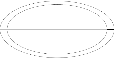
Figure 3: Mesh used for the two-dimensional example.

In Figure 4 we present the error

$$\max_{1\leq i\leq M}\left|u(r_{i})-u_{FEM}(r_{i})\right|,\qquad M:=20,$$

versus the polynomial degree $p$, in a semi-log scale. The $M$ points $r_{i}$ were uniformly distributed first on the mesh line connecting the points $(8\varepsilon,0),(1,0)$, as highlighted in Figure 3, and second on the generic line, of width approximately $8\varepsilon$, within the layer starting from the boundary point $(\sqrt{2},\sqrt{2}/2)$ at a $-45$ degree angle. Figure 4 clearly shows the robust exponential convergence in the $L^{\infty}(\Omega)$-norm of the $hp$-FEM on the Spectral Boundary Layer mesh.

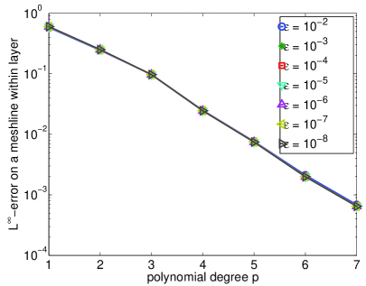
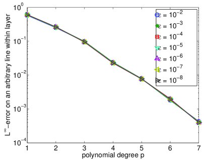
Figure 4: Maximum norm convergence of the $hp$-FEM. Left: on a meshline within the layer. Right: on a generic line within the layer.

References

- [1] N. S. Bakhvalov, Towards optimization of methods for solving boundary value problems in the presence of boundary layers, (in Russian), Zh. Vychisl. Mat. Mat. Fiz. Vol. 9, pp. 841–859 (1969).
- [2] R. Lin and M. Stynes, A balanced finite element method for singularly perturbed reaction-diffusion problems, SIAM J. Numer. Anal., Vol. 50, no.5, pp. 2729–2743 (2012).
- [3] J. M. Melenk, On the robust exponential convergence of hp finite element methods for problems with boundary layers, IMA J. Num. Anal., Vol. 17, pp. 577 – 601 (1997).
- [4] J. M. Melenk, hp-Finite Element Methods for Singular Perturbations, Vol. 1796 of Springer Lecture Notes in Mathematics, Springer Verlag, 2002.
- [5] M. J. Melenk, C. Xenophontos and L. Oberbroeckling, Robust exponential convergence of hp-FEM for singularly perturbed systems of reaction-diffusion equations with multiple scales, IMA J. Num. Anal., Vol. 33., No 2, pp. 609–628, (2013).
- [6] M. J. Melenk, C. Xenophontos and L. Oberbroeckling, Analytic regularity for a singularly perturbed system of reaction-diffusion equations with multiple scales, Advances in Computational Mathematics, Vol. 39, pp. 367–394 (2013).
- [7] J. M. Melenk and C. Schwab, hp FEM for reaction diffusion equations I: Robust exponential convergence, SIAM J. Num. Anal., Vol. 35, pp 1520–1557 (1998).
- [8] J. J. Miller, E. O’Riordan, G. I. Shishkin, Fitted Numerical Methods For Singular Perturbation Problems, World Scientific, 1996.
- [9] H. G. Roos and S. Franz, Error estimation in a balanced norm for a convection-diffusion problems with two different boundary layers, in press in Calcolo.
- [10] H. G. Roos and M. Schopf, Convergence and stability in balanced norms of finite element methods on Shishkin meshes for reaction-diffusion problems, in press in ZAMM.
- [11] H. G. Roos, M. Stynes and L. Tobiska, Robust numerical methods for singularly perturbed differential equations, Volume 24 of Springer Series in Computational Mathematics, Springer-Verlag, Berlin, 2008.
- [12] C. Schwab, p/hp Finite Element Methods, Oxford University Press, 1998.
- [13] C. Schwab and M. Suri, The p and hp versions of the finite element method for problems with boundary layers, Math. Comp. 65,pp. 1403–1429 (1996).
- [14] G. I. Shishkin, Grid approximation of singularly perturbed boundary value problems with a regular boundary layer, Sov. J. Numer. Anal. Math. Model. Vol. 4, pp. 397–417 (1989).
- [15] B. Sündermann, Lebesgue constants in Lagrangian interpolation at the Fekete points, Ergebnisberichte der Lehrstühle Mathematik III und VIII (Angewandte Mathematik) 44, Universität Dortmund, 1980.