Simultaneous Drawing of Planar Graphs
with Right-Angle Crossings and Few Bends

Abstract

Given two planar graphs that are defined on the same set of vertices, a RAC simultaneous drawing is a drawing of the two graphs where each graph is drawn planar, no two edges overlap, and edges of one graph can cross edges of the other graph only at right angles. In the geometric version of the problem, vertices are drawn as points and edges as straight-line segments. It is known, however, that even pairs of very simple classes of planar graphs (such as wheels and matchings) do not always admit a geometric RAC simultaneous drawing.

In order to enlarge the class of graphs that admit RAC simultaneous drawings, we allow edges to have bends. We prove that any pair of planar graphs admits a RAC simultaneous drawing with at most six bends per edge. For more restricted classes of planar graphs (e.g., matchings, paths, cycles, outerplanar graphs, and subhamiltonian graphs), we significantly reduce the required number of bends per edge. All our drawings use quadratic area.

1 Introduction

A simultaneous embedding of two planar graphs embeds each graph in a planar way—using the same vertex positions for both embeddings. Edges of one graph are allowed to intersect edges of the other graph. There are two versions of the problem: In the first version, called Simultaneous Embedding with Fixed Edges (Sefe), edges that occur in both graphs must be embedded in the same way in both graphs (and hence, cannot be crossed by any other edge). In the second version, simply called Simultaneous Embedding, these edges can be drawn differently for each of the graphs. Both versions of the problem have a geometric variant where edges must be drawn using straight-line segments.

Simultaneous embedding problems have been investigated extensively over the last few years, starting with the work of Brass et al. [9] on simultaneous straight-line drawing problems. Bläsius et al. [8] recently surveyed the area. For example, it is possible to decide in linear time whether a pair of graphs admits a Sefe or not, if the common graph is biconnected [1] or if it has a fixed planar embedding [2]. Furthermore, Sefe can be decided in polynomial time if each connected component of the common graph is biconnected or subcubic [30], or if it is outerplanar with cutvertices of degree at most 3 [7].

When actually drawing these simultaneous embeddings, a natural choice is to use straight-line segments. It is NP-hard to decide whether two planar graphs admit a geometric simultaneous embedding [17]. This negative results holds even if one of the input graphs is a matching [11]. In fact, only very few graphs can be drawn in this way and some existing results require exponential area. For instance, there exist a tree and a path which cannot be drawn simultaneously with straight-line segments [3], and the algorithm for simultaneously drawing a tree and a matching [11] does not provide a polynomial area bound.

A way to overcome the restrictions of straight-line drawings is to allow edges to bend. The resulting drawings with polygonal edges are called polyline drawings for short. Such drawings have been investigated by Haeupler et al. [21]. They showed that if the common graph is biconnected, then a drawing can be found in which one input graph has no bends at all and in the other input graph the number of bends per edge is bounded by the number of common vertices. Erten and Kobourov [16] showed that three bends per edge and quadratic area suffice for any pair of planar graphs (without fixed edges), and that one bend per edge suffices for pairs of trees. Kammer [26] reduced the required number of bends per edge to two for the general case of planar graphs. Grilli et al. [20] proved that every Sefe embedding of two planar graphs admits a drawing with no bends in the common edges and at most nine bends per exclusive edge. For the case that the common graph is biconnected, they reduced the number of bends to three per exclusive edge. Very recently, Frati et al. [19] improved upon these Sefe results. They reduced the bend complexity for pairs of planar graphs to 6 and for pairs of trees to 1. They also bounded the number of crossings per edge pair; to 16 and 4, respectively. In that respect, Frati et al. also improve upon a result of Chan et al. [12] who needed 24 crossings per edge pair. While Chan et al. used up to $72n$ bends per exclusive edge, they managed to keep their drawing on a grid of polynomial size ($O(n^{2})\times O(n^{2})$), which is neither the case for Frati et al. [19] nor for Grilli et al. [20]. In all these results, however, the crossing angles can be very small. Additionally, the Sefe drawings with $O(1)$ bends per edge use at least exponential space.

In this paper, we suggest a new approach that overcomes the aforementioned problems. We insist that crossings occur at right angles, thereby “taming” them. We do this while drawing all vertices and all bends on an integer grid of size $O(n)\times O(n)$ for any pair of planar $n$-vertex graphs. In a way, our results give a measure for the geometric complexity of simultaneous embeddability for various combinations of graph classes, some of which can be combined more easily (that is, with fewer bends) and some not as easily (that is, with more bends).

Let $G_{1}=(V,E_{1})$ and $G_{2}=(V,E_{2})$ be two planar graphs defined on the same vertex set and let $n=|V|$. We say that $G_{1}$ and $G_{2}$ admit a RAC simultaneous drawing (or, RacSim drawing for short) if we can place the vertices on the plane such that:

1. each edge is drawn as a polyline,

2. both graphs are drawn planar,

3. non-common edges are either disjoint or cross each other (one or several times) at right angles, and

4. common edges may be represented by the same polyline.

Note that non-common edges may not overlap. $G_{1}$ and $G_{2}$ admit a RAC simultaneous drawing with fixed edges (or, RacSefe drawing for short) if they admit a RacSim drawing with the adjusted condition (iv):

1. common edges must be represented by the same polyline.

(a) two graphs on the same vertex set

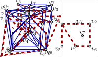
(b) a RacSim drawing

(c) a RacSefe drawing

Figure 1: (a) Two planar graphs on the same vertex set. (b) A RacSim drawing of the two graphs with at most one bend per edge. The edge $(v_{2},v_{6})$ is drawn differently in the two graphs, while the edges $(v_{3},v_{4})$ and $(v_{2},v_{3})$ are both represented by the same polyline in the two graphs. (c) A RacSefe drawing of the two graphs with up to two bends per edge.

In Figure 1, we give an example of two planar graphs on the same vertex set that admit a RacSim drawing with at most one bend per edge and a RacSefe drawing with at most two bends per edge.

Argyriou et al. [4] introduced and studied the geometric version of the RacSim drawing problem. In particular, they proved that any pair of a cycle and a matching admits a geometric RacSim drawing on an integer grid of quadratic size, while there exist a wheel and a cycle that do not admit a geometric RacSim drawing. The problem that we study in this paper was left as an open problem.

Closely related to the RacSim drawing problem is the problem of simultaneously drawing a (primal) embedded graph and its dual, so that the primal-dual edge crossings form right angles. Brightwell and Scheinermann [10] proved that this is always possible if the input graph is triconnected planar. Erten and Kobourov [15] presented an $O(n)$-time algorithm that computes a simultaneous drawing of a triconnected planar graph and its dual on an integer grid of size $O(n)\times O(n)$, where $n$ is the total number of vertices in the graph and its dual; their drawings, however, can have non-right angle crossings.

Our contribution.

Graph classes		Number of bends	Ref.	Model
planar   $+$	planar	$6+6$	Thm. 2.1	RacSim
subhamiltonian   $+$	subhamiltonian	$4+4$	Cor. 1	RacSim
outerplanar   $+$	outerplanar	$3+3$	Thm. 2.2	RacSim
cycle   $+$	cycle	$1+1$	Thm. 3.1	RacSefe
caterpillar   $+$	cycle	$1+1$	Thm. 3.2	RacSefe
four matchings		$1+1+1+1$	Thm. 3.3	RacSim
tree   $+$	matching	$1+0$	Thm. 3.4	RacSefe
wheel   $+$	matching	$2+0$	Thm. 4.1	RacSefe
outerpath   $+$	matching	$2+1$	Thm. 4.2	RacSefe

Table 1: A short summary of our results

Our main result is that any pair of planar graphs admits a RacSim drawing with at most six bends per edge. For pairs of subhamiltonian graphs and pairs of outerplanar graphs, we can reduce the required number of bends per edge to four and three, respectively; see Section 2. (Recall that a subhamiltonian graph is a subgraph of a planar Hamiltonian graph.) Then, we turn our attention to pairs of more restricted graph classes where we can guarantee RacSim and RacSefe drawings with one bend per edge or two bends per edge; see Sections 3 and 4, respectively. Table 1 summarizes our results. Note that all our algorithms run in linear time, with the exception of the algorithm for an outerpath and a matching (see Theorem 4.2), which runs in $O(n\log n)$ time. The produced drawings fit on integer grids of quadratic size. The main approach of all our algorithms is to find linear orders on the vertices of the two graphs and then to compute the exact coordinates of the vertices of both graphs based on these orders. These drawings may contain non-rectilinear segments (referred to as slanted segments, for short), but all crossings in our drawings appear between horizontal and vertical edge segments and are therefore at right angle.

2 RacSim Drawings of General Graphs

In this section, we study general planar graphs and show how to efficiently construct RacSim drawings in quadratic area, with few bends per edge. We prove that two planar graphs on a common set of vertices admit a RacSim drawing with six bends per edge (Theorem 2.1). We lower the required number of bends per edge to $4$ for pairs of subhamiltonian graphs (Corollary 1), and to $3$ for pairs of outerplanar graphs (Theorem 2.2). Note that the class of subhamiltonian graphs is equal to the class of 2-page book-embeddable graphs, and the class of outerplanar graphs is equal to the class of 1-page book-embeddable graphs [6].

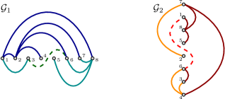
Figure 2:  Drawings of two planar graphs by Kaufmann and Wiese [27].

Central to our approach is an algorithm by Kaufmann and Wiese [27] that embeds any planar graph such that vertices are mapped to points on a horizontal line (the so-called spine) and each edge crosses the spine at most once; see Figure 2. If one replaces each spine crossing with a dummy vertex, then a linear order of the vertices (both original and dummy) is obtained with the property that every edge is either completely above or completely below the spine. In order to determine the exact locations of the vertices of the two given graphs in our problem, we use the linear order induced by the first graph to compute the $x$-coordinates and the linear order induced by the second graph to compute the corresponding $y$-coordinates. (Note that this approach has been used for simultaneous drawing problems before [16].) Then, we draw the edges of both graphs, so that all edges-crossings

1. are restricted between vertical and horizontal edge-segments, that is, slanted edge-segments are crossing-free, and

2. appear in the interior of the smallest axis-aligned rectangle containing all vertices.

Theorem 2.1

Two planar graphs on a common set of $n$ vertices admit a RacSim drawing on an integer grid of size $(14n-26)\times(14n-26)$ with six bends per edge. The drawing can be computed in $O(n)$ time.

Proof

Let $\mathcal{G}_{1}=(V,E_{1})$ and $\mathcal{G}_{2}=(V,E_{2})$ be planar graphs. For $m\in\{1,2\}$, let $\xi_{m}$ be an embedding of $\mathcal{G}_{m}$ according to the algorithm of Kaufmann and Wiese [27]; see Figure 2. As explained before, we subdivide all edges of $\mathcal{G}_{m}$ that cross the spine in $\xi_{m}$ by introducing a dummy vertex at the point where it crosses the spine. Let $\mathcal{G}_{m}^{\prime}=(V_{m}^{\prime},E_{m}^{\prime})=(V\cup V_{m},A_{m}\cup B_{m})$ be the resulting graph, where $V_{m}$ is the set of dummy vertices in $\mathcal{G}_{m}^{\prime}$, $A_{m}$ is the set of edges that are drawn completely above the spine and $B_{m}$ is the set of edges that are drawn completely below the spine. Let $\xi_{m}^{\prime}$ be the embedding of $\mathcal{G}_{m}^{\prime}$.

Now we show how to determine the $x$-coordinates of the vertices in $V_{1}^{\prime}$ by assigning the vertices to the columns of a grid; the $y$-coordinates of the vertices in $V_{2}^{\prime}$ are determined analogously. Let $n_{1}^{\prime}$ be the number of vertices in $V_{1}^{\prime}$ and let $v_{1}\rightarrow v_{2}\rightarrow\dots\rightarrow v_{n_{1}^{\prime}}$ be the linear order of the vertices of $V_{1}^{\prime}$ along the spine in $\xi_{1}^{\prime}$. We start by placing $v_{1}$. Between any two consecutive vertices $v_{i}$ and $v_{i+1}$, we reserve several columns for the bends of the edges incident to $v_{i}$ and $v_{i+1}$; see Figure 3. The columns are used (in the given order) for the following purposes:

1. for the first bend on all edges in $A_{2}$ leaving $v_{i}$,

2. for the first vertical segment of each edge $(v_{i},v_{j})\in E_{1}^{\prime}$ with $j>i$,

3. for the last vertical segment of each edge $(v_{k},v_{i+1})\in E_{1}^{\prime}$ with $k\leq i$, and

4. for the last bend on all edges in $B_{2}$ entering $v_{i+1}$.

Note that we can save some columns reserved for (ii) and (iii) because an edge in $A_{1}$ and an edge in $B_{1}$ can use the same column for their bend.

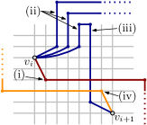
Figure 3: Reserving additional columns between $v_{i}$ and $v_{i+1}$.

With this procedure we fully specify the $x$-coordinates of the vertices in $V_{1}^{\prime}$; the $y$-coordinates of the vertices in $V_{2}^{\prime}$ are determined analogously. Let $R$ be the smallest axis-aligned rectangle that contains all vertices of the common vertex set of $\mathcal{G}_{1}^{\prime}$ and $\mathcal{G}_{2}^{\prime}$ (the gray rectangle in Figure 4(a)). Note that the $y$-coordinates of the dummy vertices of $V_{1}^{\prime}$ and the $x$-coordinates of the dummy vertices of $V_{2}^{\prime}$ have not been determined by the algorithm so far. They can be set arbitrarily, as long as the corresponding vertices are inside $R$.

We proceed to describe how to draw the edges of graph $\mathcal{G}_{1}^{\prime}$ with at most four bends per edge such that all edge segments of $\mathcal{G}_{1}^{\prime}$ in $R$ are either vertical or of $y$-length exactly 1; see Figure 4(b). The edges of graph $\mathcal{G}_{2}$ are drawn analogously (rotated by $90^{\circ}$). First, we draw the edges $(v_{i},v_{j})\in A_{1}$ with $i<j$ in a nested order: When we draw the edge $(v_{i},v_{j})$, there is no edge $(v_{k},v_{l})\in A_{1}$ with $k\leq i$ and $l\geq j$ that has not already been drawn. Recall that the first column to the right and the first column to the left of every vertex is reserved for the edges in $E_{2}$, hence we assume that they are already used. We draw $(v_{i},v_{j})$ with at most four bends as follows. We start with a slanted segment incident to $v_{i}$ that has its other endpoint in the row above $v_{i}$ and in the first unused column that does not lie to the left of $v_{i}$. We follow with an upward vertical segment that leaves $R$. We add a horizontal segment above $R$; the row of this segment is determined by the nesting in the book embedding of $\mathcal{G}^{\prime}_{1}$. In the last unused column that does not lie to the right of $v_{j}$, we add a vertical segment that ends one row above $v_{j}$. We finish the edge with a slanted segment that has its endpoint in $v_{j}$. We draw the edges in $B_{1}$ symmetrically, with the horizontal segment below $R$.

(a) $\mathcal{G}_{1}$

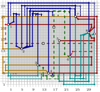
(b) $\mathcal{G}_{1}$ and $\mathcal{G}_{2}$

Figure 4: RacSim drawings of the graphs $\mathcal{G}_{1}$ and $\mathcal{G}_{2}$ (see Figure 2) with at most six bends per edge, generated by our algorithm. The edges that cross the spine are drawn dashed; the dummy vertices on these edges are drawn as squares.

Note that this algorithm always uses the top and the bottom port of a vertex $v$ if there is at least one edge incident to $v$ in $A_{1}$ and $B_{1}$ respectively. The edges incident to a dummy vertex use precisely the top and the bottom port: Dummy vertices have exactly one incident edge in $A_{1}$ and one in $B_{1}$. We create a drawing of $\mathcal{G}_{1}$ and $\mathcal{G}_{2}$ with at most 6 bends per edge by bypassing (that is, smoothing out) the dummy vertices. This does not change the drawing.

By construction, all edge segments of $E_{1}$ inside $R$ are either vertical segments or slanted segments of $y$-length 1. Symmetrically, all segments of $E_{2}$ inside $R$ are either horizontal segments or slanted segments of $x$-length 1. Thus, the slanted segments cannot intersect. All crossings inside $R$ occur between a horizontal and a vertical segment, and thus form right angles. Also, there are no segments in $E_{1}$ that lie to the left or to the right of $R$, and there are no segments in $E_{2}$ that lie above or below $R$. Hence, there are no crossings outside $R$, which guarantees that the constructed drawing of $\mathcal{G}_{1}$ and $\mathcal{G}_{2}$ is a RacSim drawing.

We now count the columns used by the drawing. For the leftmost and the rightmost vertex, we reserve one additional column for its incident edges in $E_{2}$; for the remaining vertices, we reserve two such columns. For each edge in $E_{1}$, we use up to three columns: one for each endpoint of the slanted segment at each vertex and one for the vertical segment that crosses the spine, if it exists. Recall that at least one edge per vertex does not need a slanted segment. For each edge in $E_{2}$, we need at most one column for the vertical segment to the side of $R$. Since there are at most $3n-6$ edges, we need at most

$$3n-2+3\cdot(3n-6)-n+3n-6=14n-26$$

columns. By symmetry we need the same number of rows.

The algorithm of Kaufmann and Wiese computes a drawing with at most 3 bends per edge in $O(n)$ time. We can compute the nested order of the edges in linear time from the embedding, as the circular order of the edges around a vertex gives a hierarchical order on the edges that describes the nested order of the edges. Thus, our algorithm also runs in $O(n)$ total time.

We can improve the result of Theorem 2.1 for subhamiltonian graphs, which admit 2-page book embeddings in which no edges cross the spine [6]. Since those edges are the only ones that need six bends, the number of bends per edge is reduced to four. The number of columns and rows are also reduced by one per edge. This is summarized in the following corollary. Note, however, that it is NP-hard to decide whether a given planar graph is subhamiltonian, even for maximal planar graphs [31]. A 2-page book embedding can be found in linear time, if the ordering of the vertices along the spine is given [22]. Several classes of graphs are known to be (sub)hamiltonian, for example 4-connected planar graphs [29], planar graphs without separating triangles [25], Halin graphs [13], planar graphs with maximum degree 3 or 4 [5, 24].

Corollary 1

Two subhamiltonian graphs on a common set of $n$ vertices admit a RacSim drawing on an integer grid of size $(11n-32)\times(11n-32)$ with four bends per edge. The algorithm runs in $O(n)$ time if the subhamiltonian cycles of both graphs are given.

We use even fewer bends for a RacSim drawing of two outerplanar graphs. This is based on a decomposition of each of the graphs into two forests. The following lemma shows that we can do this in linear time.

Lemma 1

Every outerplanar graph can be decomposed into two forests. This decomposition can be computed in linear time.

Proof

It follows by Nash-Williams’ formula [28] that every outerplanar graph has arboricity 2, that is, it can be decomposed into two forests. To prove the linear running time, we first assume biconnectivity and augment the input graph to a maximal outerplanar graph. Now, if we add a new vertex that is incident to all vertices of the graph, the result is a maximal planar graph which can be decomposed into three trees [18], so that one of them is a star incident to the newly added vertex. Hence, the removal of this vertex yields a decomposition into two trees. The desired decomposition into two forests follows from the removal of the edges added to augment the graph to maximal outerplanar. For an outerplanar graph that is not biconnected, we have to compute the aforementioned decomposition for each of its biconnected components individually. Since the biconnected components of a graph form a tree (the so-called BC-tree), the structure of the overall decomposition is not affected; it still consists of two forests. The overall decomposition can be computed in linear time since both the decomposition of a maximal planar graph into three trees and the computation of the biconnected components of the outerplanar input graph can be found in linear time.

With this lemma, we can further improve the required number of bends per edge to three for outerplanar graphs. (Recall that all outerplanar graphs are 1-page book embeddable.) We will use the order of the vertices on the spine of a 1-page book embedding to compute a 2-page book embedding in which every edge uses a rectilinear port at one of its endpoints, enabling us to omit one of its bends.

Theorem 2.2

Two outerplanar graphs on a common set of $n$ vertices admit a RacSim drawing on an integer grid of size $(7n-10)\times(7n-10)$ with three bends per edge. The drawing can be computed in $O(n)$ time.

Proof

Let $\mathcal{O}_{1}=(V,E_{1})$ and $\mathcal{O}_{2}=(V,E_{2})$ be the given outerplanar graphs. We will embed $\mathcal{O}_{1}$ and $\mathcal{O}_{2}$ on two pages with one forest per page.

To do so, we first create 1-page book embeddings for $\mathcal{O}_{1}$ and for $\mathcal{O}_{2}$ using the linear time algorithm of Heath [23]. This gives the orders of the vertices of both graphs along the spine. It follows by Corollary 1 that, by using the algorithm described in the proof of Theorem 2.1, we can create a RacSim drawing of $\mathcal{O}_{1}$ and $\mathcal{O}_{2}$ with at most four bends per edge. We will now show how to adjust the algorithm to reduce the number of bends by one.

We decompose $\mathcal{O}_{1}$ into two forests $A_{1}$ and $B_{1}$ according to Lemma 1. We will draw the edges of $A_{1}$ above the spine and the edges $B_{1}$ below the spine. By rooting the trees in $A_{1}$ in arbitrary vertices, we can direct each edge such that every vertex has exactly one incoming edge. Recall that, in the drawing produced in Theorem 2.1, one edge per vertex can use its top port. We adjust the algorithm such that every directed edge $(v,w)$ enters vertex $w$ from its top port. To do so, we draw the edge as follows. We start with a slanted segment of $y$-length 1. We follow with a vertical segment to the top, a horizontal segment that ends directly above $w$, and finish the edge with a vertical segment that enters $w$ in the top port. We use the same approach for the edges in $B_{1}$, using the bottom port and treat the second outerplanar graph $\mathcal{O}_{2}$ analogously.

Since every port of a vertex is only used once, the drawing has no overlaps. We now analyze the number of columns used. For every vertex except for the leftmost and rightmost, two additional columns are reserved for the edges in $E_{2}$; for the remaining two vertices, we reserve a single additional column. The edges in $E_{1}$ now only need one column for the bend of the single slanted segment. For every edge in $E_{2}$, we need up to one column for the vertical segment to the side of $R$. Since there are at most $2n-4$ edges, our drawing needs $3n-2+2n-4+2n-4=7n-10$ columns. Analogously, we can show that the algorithm needs $7n-10$ rows. Since the decomposition can be computed in $O(n)$ time, our algorithm also requires $O(n)$ time.

3 RacSim and RacSefe Drawings with One Bend per Edge

In this section, we study simple classes of planar graphs and show how to efficiently construct RacSim and/or RacSefe drawings with one bend per edge in quadratic area. In particular, we prove that two cycles (four matchings, resp.) on a common set of $n$ vertices admit a RacSefe (RacSim, resp.) drawing on an integer grid of size $2n\times 2n$; see Theorem 3.1 (Theorem 3.3, resp.). If the input to our problem is a caterpillar and a cycle, then we can compute a RacSefe drawing with one bend per edge on an integer grid of size $(2n-1)\times 2n$; see Theorem 3.2. For a tree and a cycle, we can construct a RacSefe drawing with one bend per tree edge and no bends in the matching edges on an integer grid of size $n\times(n-1)$; see Theorem 3.4.

In the next proof and in a few more places throughout this paper, we use the following common notation. For any real $x$, let the sign of $x$, $\operatorname{sgn}(x)$, be 0 if $x=0$, $1$ if $x>0$, and $-1$ if $x<0$.

Lemma 2

Two paths on a common set of $n$ vertices admit a RacSefe drawing on an integer grid of size $2n\times 2n$ with one bend per edge. The drawing can be computed in $O(n)$ time.

Proof

Let $\mathcal{P}_{1}=(V,E_{1})$ and $\mathcal{P}_{2}=(V,E_{2})$ be the given paths. To keep the description simple, we first assume that $\mathcal{P}_{1}$ and $\mathcal{P}_{2}$ do not share edges. Following standard practices from the literature (see for example Brass et al. [9]), we draw $\mathcal{P}_{1}$ $x$-monotone and $\mathcal{P}_{2}$ $y$-monotone. This ensures that the drawing of the paths will individually be planar. We will now describe how to compute the exact coordinates of the vertices and how to draw the edges of $\mathcal{P}_{1}$ and $\mathcal{P}_{2}$, such that all crossings are at right angles and, more importantly, that no edge segments overlap.

For $m\in\{1,2\}$ and any vertex $v\in V$, let $\pi_{m}(v)$ be the position of $v$ in $\mathcal{P}_{m}$. Then, $v$ is drawn at the point $p(v)=(2\pi_{1}(v)-1,2\pi_{2}(v)-1)$; see Figure 5. It remains to determine, for each edge $e=(v,v^{\prime})$, where to place its bend. First, assume that $e\in E_{1}$ and that $e$ is directed from its left endpoint, say $v$, to its right endpoint, say $v^{\prime}$. Then we place the bend to the left of $v^{\prime}$, and one row above or below it depending on which direction the edge is coming from. To be exact, we place it at $p(v^{\prime})-(2,\operatorname{sgn}(y(v^{\prime})-y(v)))$. Second, assume that $e\in E_{2}$ and $e$ is directed from its bottom endpoint, say $v$, to its top endpoint, say $v^{\prime}$. Then, we place the bend at $p(v^{\prime})-(\operatorname{sgn}(x(v^{\prime})-x(v)),2)$.

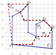
Figure 5: RacSefe drawings with one bend per edge: two paths $\mathcal{P}_{1}$ (thin solid) and $\mathcal{P}_{2}$ (bold dashed) and two cycles $\mathcal{C}_{1}=\mathcal{P}_{1}+(v_{1},v_{6})$ and $\mathcal{C}_{2}=\mathcal{P}_{2}+(v_{1},v_{3})$

The area required by the drawing is $(2n-1)\times(2n-1)$. An edge of $\mathcal{P}_{1}$ leaves its left endpoint vertically and enters its right endpoint with a slanted segment of $x$-length 1 and $y$-length 2. Similarly, an edge of $\mathcal{P}_{2}$ leaves its bottom endpoint horizontally and enters its top endpoint with a slanted segment of $x$-length 2 and $y$-length 1. Hence, the slanted segments cannot be involved in crossings or overlaps. Since $\mathcal{P}_{1}$ and $\mathcal{P}_{2}$ are $x$- and $y$-monotone, respectively, it follows that all crossings must involve a vertical edge segment of $\mathcal{P}_{1}$ and a horizontal edge segment of $\mathcal{P}_{2}$, which is at right angle. The runtime is clearly linear.

Finally, we show that our algorithm supports the Sefe model. Assume that $\mathcal{P}_{1}=(V,E_{1})$ and $\mathcal{P}_{2}=(V,E_{2})$ share edges, and let $e=(v,v^{\prime})$ be an edge that belongs to both input paths. Our algorithm automatically places $v$ and $v^{\prime}$ at consecutive $x$- and $y$-coordinates and draws $e$ as a diagonal of $x$- and $y$-length 2 in both graphs, which cannot be involved in a crossing.

We say that an edge uses the bottom/left/right/top port of a vertex if it enters the vertex from the bottom/left/right/top.

Theorem 3.1

Two cycles on a common set of $n$ vertices admit a RacSefe drawing on an integer grid of size $2n\times 2n$ with at most one bend per edge. The drawing can be computed in $O(n)$ time.

Proof

Let $\mathcal{C}_{1}=(V,E_{1})$ and $\mathcal{C}_{2}=(V,E_{2})$ be the given cycles and assume first that $\mathcal{C}_{1}$ and $\mathcal{C}_{2}$ do not share edges. Let $v\in V$ be an arbitrary vertex. We temporarily delete one edge $(v,w_{1})\in E_{1}$ from $\mathcal{C}_{1}$ and one edge $(v,w_{2})\in E_{2}$ from $\mathcal{C}_{2}$ (refer to the edges $(v_{1},v_{3})$ and $(v_{1},v_{6})$ in Figure 5). This results into two paths $\mathcal{P}_{1}=\langle v,\ldots,w_{1}\rangle$ and $\mathcal{P}_{2}=\langle v,\ldots,w_{2}\rangle$. We use the algorithm of Lemma 2 to construct a RacSim drawing of $\mathcal{P}_{1}$ and $\mathcal{P}_{2}$ on an integer grid of size $(2n-1)\times(2n-1)$. Since $v$ is the first vertex in both paths, it is placed at the bottom-left corner of the bounding box containing the drawing. Since $w_{1}$ and $w_{2}$ are the last vertices in $\mathcal{P}_{1}$ and $\mathcal{P}_{2}$, respectively, $w_{1}$ is placed on the right side, and $w_{2}$ on the top of the bounding box. By construction, the bottom port of $w_{1}$ and the left port of $w_{2}$ are both unoccupied. Hence, the edges $(v,w_{1})$ and $(v,w_{2})$ that form $\mathcal{C}_{1}$ and $\mathcal{C}_{2}$ can be drawn with a single bend at points $(2n-1,0)$ and $(0,2n-1)$ respectively; see Figure 5. Since both edges are completely outside of the bounding box containing the drawing, neither is involved in crossings. The total area of the drawing gets larger by a single unit in each dimension. The runtime bound is unaffected.

It remains to consider the case that $\mathcal{C}_{1}$ and $\mathcal{C}_{2}$ share edges. Since $\mathcal{P}_{1}$ and $\mathcal{P}_{2}$ already support the Sefe model, it suffices to consider the case that a closing edge $(v,w_{1})$ or $(v,w_{2})$ is also contained in the other graph. Since the closing edges are drawn planar, we can simply use their drawing in both graphs and remove the corresponding edge from the path. Thus, the drawing supports the Sefe model.

Theorem 3.2

A caterpillar and a cycle on a common set of $n$ vertices admit a RacSefe drawing on an integer grid of size $(2n-1)\times 2n$ with one bend per edge. The drawing can be computed in $O(n)$ time.

Proof

Let $\mathcal{A}=(V,E_{\mathcal{A}})$ be the given caterpillar and $\mathcal{C}=(V,E_{\mathcal{C}})$ the given cycle. Similar to the previous proofs, we will first prove that $\mathcal{A}$ and $\mathcal{C}$ admit a RacSim drawing, assuming that they do not share edges. We postpone the case where $\mathcal{A}$ and $\mathcal{C}$ share edges for later. A caterpillar can be decomposed into a path, called its spine, and a set of leaves connected to the path, called its legs. Let $v_{1},v_{2},\ldots,v_{n}$ be the vertex set of $\mathcal{A}$ ordered as follows (see Figure 6): Starting from an endpoint of the spine of $\mathcal{A}$, we traverse the caterpillar such that we visit all legs incident to a spine vertex before moving on to the next spine vertex. This order defines the $x$-order of the vertices in the output drawing.

As in the proof of Theorem 3.1, we temporarily delete an edge of $\mathcal{C}$ incident to $v_{1}$ (see the thin dashed edge in Figure 6) and obtain a path which we denote by $\mathcal{P}=(V,E_{\mathcal{P}})$. For any vertex $v_{i}\in V$, let $\pi(v_{i})$ be the position of $v_{i}$ in $\mathcal{P}$. The map $\pi$ determines the $y$-order of the vertices in our drawing. For $i\in\{1,2,\ldots,n\}$, we draw vertex $v_{i}$ at point $p(v_{i})=(2i-1,2\pi(v_{i})-1)$. It remains to determine, for each edge $e=(v,v^{\prime})$, where to place its bend. First, assume that $e\in E_{\mathcal{P}}$ and that $e$ is directed from its bottom endpoint, say $v$, to its top endpoint, say $v^{\prime}$ (see the bold dashed edges in Figure 6). Then, we place the bend at $p(v)+(\operatorname{sgn}(x(v^{\prime})-x(v)),2)$. Second, assume that $e\in E_{\mathcal{A}}$ and $e$ is directed from its left endpoint, say $v$, to its right endpoint, say $v^{\prime}$ (see the solid edges in Figure 6). Then, we place the bend at $(x(v^{\prime}),y(v)+\operatorname{sgn}(y(v^{\prime})-y(v))$.

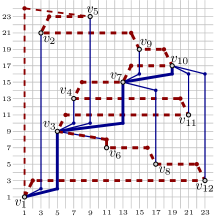
Figure 6: A RacSefe drawing of a caterpillar (solid; its spine is drawn bold) and a cycle (dashed)

The approach described above ensures that $\mathcal{P}$ is drawn $y$-monotone, hence planar. The spine of $\mathcal{A}$ is drawn $x$-monotone. The legs of a spine vertex of $\mathcal{A}$ are drawn to the right of their parent spine vertex and to the left of the next vertex along the spine. Hence, $\mathcal{A}$ is drawn planar as well. The slanted segments of $\mathcal{A}$ have $y$-length 1, while the slanted segments of $\mathcal{P}$ have $x$-length 1. Thus, they cannot be involved in crossings, which implies that all crossings form right angles.

It remains to draw the edge $e$ in $E_{\mathcal{C}}\setminus E_{\mathcal{P}}$. Recall that $e$ is incident to $v_{1}$, which lies at the bottom-left corner of the bounding box containing our drawing. Let $v_{j}$ be the other endpoint of $e$. Since $\pi(v_{j})=n$, vertex $v_{j}$ lies at the top of the bounding box. As the top port of $v_{1}$ is not used, we can draw the first segment of $e$ vertical, bending at $(1,2n)$; see the thin dashed edge in Figure 6.

To complete the proof of this theorem, it remains to show that our algorithm supports the Sefe model. Suppose that there is an edge $e=(v,v^{\prime})$ that belongs to both $\mathcal{A}$ and $\mathcal{C}$. Our algorithm places $v$ and $v^{\prime}$ at consecutive $y$-coordinates. Thus, the drawing of $e$ in $\mathcal{A}$ consists of a slanted and a vertical segment of $y$-length 1 each. This drawing of $e$ in $\mathcal{A}$ is not crossed by any edge of $E_{\mathcal{C}}$, so $e$ can be drawn in the same way for both graphs.

Clearly, the area of the drawing is $(2n-1)\times 2n$, and the runtime is linear.

Theorem 3.3

Four matchings on a common set of $n$ vertices admit a RacSim drawing on an integer grid of size $2n\times 2n$ with at most one bend per edge. The drawing can be computed in $O(n)$ time.

Proof

Let $\mathcal{M}_{1}=(V,E_{1})$, $\mathcal{M}_{2}=(V,E_{2})$, $\mathcal{M}_{3}=(V,E_{3})$ and $\mathcal{M}_{4}=(V,E_{4})$ be the given matchings. Without loss of generality, we assume that all matchings are perfect; otherwise, we augment them to perfect matchings. Let $\mathcal{M}_{1,2}=(V,E_{1}\cup E_{2})$ and $\mathcal{M}_{3,4}=(V,E_{3}\cup E_{4})$. Since $\mathcal{M}_{1}$ and $\mathcal{M}_{2}$ are defined on the same vertex set, $\mathcal{M}_{1,2}$ is a $2$-regular graph. Thus, each connected component of $\mathcal{M}_{1,2}$ corresponds to a cycle of even length which alternates between edges of $\mathcal{M}_{1}$ and $\mathcal{M}_{2}$; see Figure 7. The same holds for $\mathcal{M}_{3,4}$. We will determine the $x$-coordinates of the vertices from $\mathcal{M}_{1,2}$, and the $y$-coordinates from $\mathcal{M}_{3,4}$.

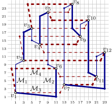
Figure 7: A RacSim drawing of four matchings: $\mathcal{M}_{1}$ (solid-plain), $\mathcal{M}_{2}$ (solid-bold), $\mathcal{M}_{3}$ (dashed-plain), and $\mathcal{M}_{4}$ (dashed-bold)

We start by choosing an arbitrary vertex $v\in V$. Let $\mathcal{C}$ be the cycle of $\mathcal{M}_{1,2}$ containing vertex $v$. We determine the $x$-coordinates of the vertices of $\mathcal{C}$ by traversing it in some direction, starting from vertex $v$. For each vertex $u$ in $\mathcal{C}$, let $\pi_{1}(u)$ be the discovery time of $u$ according to this traversal, with $\pi_{1}(v)=0$. We set $x(u)=2\pi_{1}(u)+1$. After doing this, we determine the $y$-coordinates of all vertices that lie on cycles in $\mathcal{M}_{3,4}$ that contain at least one vertex of $\mathcal{C}$ (that is, cycles in $\mathcal{M}_{3,4}$ that contain a vertex for which the $x$-coordinate has been determined). Call these cycles $\mathcal{C}_{1},\ldots,\mathcal{C}_{k}$, ordered as follows. For $i\in\{1,\ldots,k\}$, let $a_{i}$ be the anchor of $\mathcal{C}_{i}$, that is, the vertex with the smallest determined $x$-coordinate of all vertices in $\mathcal{C}_{i}$. Then, $x(a_{1})<\ldots<x(a_{k})$. In what follows, we start with the first cycle $\mathcal{C}_{1}$ of the computed order and determine the $y$-coordinates of its vertices. To do so, we traverse $\mathcal{C}_{1}$ in some direction, starting from its anchor vertex $a_{1}$. For each vertex $u$ in $\mathcal{C}_{1}$, let $\pi_{2}(u)$ be the discovery time of $u$ according to this traversal, with $\pi_{2}(a_{1})=0$. Then, we set $y(u)=2\pi_{2}(u)+1$. We proceed analogously with the remaining cycles $\mathcal{C}_{i}$, $i=2,\ldots,k$, setting $\pi_{2}(a_{i})=\max_{u\in\mathcal{C}_{i-1}}\pi_{2}(u)+1$.

After this step, there are no vertices for which only the $x$-coordinate has been determined. However, there might exist vertices where only the $y$-coordinate has been determined. If this is the case, we repeat the aforementioned procedure to determine the $x$-coordinates of the vertices of all cycles of $\mathcal{M}_{1,2}\setminus\mathcal{C}$ that have at least one vertex with a determined $y$-coordinate, but without determined $x$-coordinates. If there are no vertices with only one determined coordinate left, either all coordinates are determined, or we restart this procedure with another arbitrary vertex that has no determined coordinates. Thus, our algorithm guarantees that the $x$- and $y$-coordinate of all vertices are eventually determined.

Note that for each cycle in $\mathcal{M}_{1,2}$ there is exactly one edge $e=(v,v^{\prime})$ with $\pi_{1}(v^{\prime})>\pi_{1}(v)+1$. We call this the closing edge. Analogously, for each cycle in $\mathcal{M}_{3,4}$, there is exactly one closing edge $e=(u,u^{\prime})$ with $\pi_{2}(u^{\prime})>\pi_{2}(u)+1$.

Finally we determine, for each edge $e=(v,v^{\prime})$, where to place its bend. First, assume that $e\in E_{1}\cup E_{2}$ and that $e$ is directed from its left endpoint, say $v$, to its right endpoint, say $v^{\prime}$. If $e$ is not a closing edge, we place the bend at $(x(v^{\prime})-2,y(v^{\prime})-\operatorname{sgn}(y(v^{\prime})-y(v))$. Otherwise, we place the bend at $(x(v^{\prime}),y(v)-1)$. Second, assume that $e\in E_{3}\cup E_{4}$ and $e$ is directed from its bottom endpoint, say $v$, to its top endpoint, say $v^{\prime}$. If $e$ is not a closing edge, we place the bend at $(x(v^{\prime})-\operatorname{sgn}(x(v^{\prime})-x(v)),x(v^{\prime})-2)$. Otherwise, we place the bend at $(x(v)-1,y(v^{\prime}))$; see Figure 7.

Our choice of coordinates guarantees that the $x$-coordinates of the cycles of $\mathcal{M}_{1,2}$ and the $y$-coordinates of the cycles of $\mathcal{M}_{3,4}$ form disjoint intervals. Thus, the area below a cycle of $\mathcal{M}_{1,2}$ and the area to the left of a cycle of $\mathcal{M}_{3,4}$ are free from vertices. Hence, the slanted segments of the closing edges cannot have a crossing that violates the RAC restriction. The total area required by the drawings is $2n\times 2n$. The running time is linear.

We now detail how to compute a RacSefe drawing of a rooted tree and a matching with one bend per tree edge and no bends on matching edges. Figure 8 shows an example output of our algorithm. Our layout algorithm is inspired by an algorithm for drawing a geometric simultaneous embedding of a tree and a matching by Cabello et al. [11], which in turn goes back to an algorithm of Di Giacomo et al. [14]. Cabello et al. draw edges straight (that is, no bends), but their crossing angles are not necessarily right. We recall some of their notation that we will then use for our purposes.

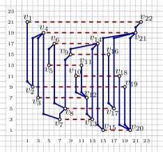
Figure 8: A RacSefe drawing of a tree (solid; rooted in $r$) and a matching (dashed). For each of the three subtrees hanging off vertex $s$ we used a different color; the subtrees occupy disjoint $x$-intervals (marked below the drawing).

Cabello et al. draw the edges of the matching horizontally. They partition the matching into a top group and a bottom group. Within the top group, they place the edges from top to bottom; vice versa within the bottom group. Once a matching edge is assigned to one of the two groups, the edge and its endpoints are called placed.

The assignment of the edges to the groups is iterative. In each step, the placed vertices induce an edge partition of the tree into connected components (subtrees); each component up to and including the placed vertices is called a rope. If a rope with three placed vertices exists, the vertex that lies on all three paths between these placed vertices is called a splitter; see Figure 9(a). Cabello et al. showed that placing a vertex creates at most one splitter and that placing a splitter does not create a new one.

Now, we are ready to present our algorithm in detail.

Theorem 3.4

A tree and a matching on a common set of $n$ vertices admit a RacSefe drawing on an integer grid of size $n\times(n-1)$ with one bend per tree edge and no bends on matching edges. The drawing can be computed in $O(n)$ time.

Proof

We first consider the case where the input graphs do not share edges. We root the given tree in an arbitrary leaf $r$, which yields a directed tree $\mathcal{T}$. We will obtain the $x$-coordinates of the vertices from a particular post-order traversal of this directed tree. As a consequence, all children of a vertex are placed to its left, and disjoint subtrees are placed in disjoint $x$-intervals. By adding dummy edges, we augment the given matching to a perfect matching if $n$ is even, or to a near-perfect matching if $n$ is odd. Let $\mathcal{M}$ be the augmented matching. After the algorithm terminates, these dummy edges can be safely removed. In order to compute a RacSefe drawing of $\mathcal{T}$ and $\mathcal{M}$, we follow an approach that is based on the one of Cabello et al. The difference is that (a) rather than placing ropes in disjoint parallelograms, we place subtrees into disjoint axis-parallel rectangles, and (b) the assignment of matching edges to the two groups is much simpler.

(a) The placed vertices (black) induce three ropes; $v$ is a splitter.

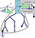
(b) Vertex $w$ has been placed at the top in the previous step, creating a splitter $v$ that will now be placed at the bottom.

Figure 9: Definition and placement of a splitter

First, we show how to compute the $y$-coordinates of the vertices. Each edge of $\mathcal{M}$ is drawn horizontally at a unique odd $y$-coordinate between $1$ and $n-1$. The coordinates are determined as follows. We start by putting the matching edge containing the root of $\mathcal{T}$ into the top group. Within the top group, the edges are assigned to odd rows, from top to bottom, starting from row $n-2$ if $n$ is odd, or $n-1$ otherwise. In the bottom group, the edges are also assigned to odd rows, but from bottom to top, starting from row 1. In this way, a matching edge is always assigned to an odd row between 1 and $n-1$. Thus, our drawing needs at most $n-1$ rows. In the following we show how to determine the group into which a matching edge goes. There are two cases.

If there is no splitter, the algorithm finds an unplaced vertex that has a tree edge to a placed vertex, and adds its matching edge to the top group. This creates at most one splitter since one of the placed vertices is adjacent to a vertex that has already been placed. Hence, whenever a new matching edge is placed, there will be at most one splitter in the graph.

Now, assume that a splitter exists. Call it $v$. For any subtree, we call the unique vertex with no incoming edge its local root. Since we start by drawing the root of $\mathcal{T}$, every vertex lies in a rope that has its local root placed. Let $T_{1}(v),\dots,T_{k}(v)$ be the subtrees of $\mathcal{T}$ hanging off $v$; see the left drawing of Figure 9(b). Then, $v$ is a splitter if and only if there are two subtrees $T_{i}(v)$ and $T_{j}(v)$ with at least one placed vertex, one of which has been placed in the last step. Without loss of generality, let $w\in T_{i}(v)$ be this vertex. If $w$ was added to the top group, we add $v$ to the bottom group; otherwise, we add $v$ to the top group. Thus, the vertices of the subtrees $T_{l}(v)$ with $l\neq j$ will be placed either all above or all below $v$; see Figure 9(b).

Next, we describe how to determine the $x$-coordinates of the vertices. We proceed inductively. For each non-leaf vertex, we compute an order of the subtrees that hang off this vertex. This order determines the disjoint $x$-intervals into which we place the subtrees. Let $v$ be a vertex that is placed in an induction step. We traverse the path from $v$ to the root of the rope it lies on. For every vertex $u$ on this path, we determine the order of the subtrees of its children as follows. Let $T_{1}(u),\ldots,T_{\ell}(u)$ be the subtrees hanging off $u$, assuming $v\in T_{1}(u)$. If $v$ is the only placed successor of vertex $u$, then we assign the order $x(T_{1}(u))<\ldots<x(T_{\ell}(u))$ to the $x$-intervals of the subtrees; otherwise, an order has already been determined. When the algorithm is done, we know the order of the subtrees for every vertex on this path. In particular, we know the $x$-interval of the subtree rooted in $v$. We assign the largest $x$-coordinate of this interval to $v$.

Now, we show how to draw the edges. Let $(u,v)$ be a directed edge of $\mathcal{T}$. We draw $(u,v)$ with a slanted segment of $y$-length 1 at vertex $u$ and a vertical segment at vertex $v$. The bend of edge lies at $(x(v),y(v)+\operatorname{sgn}(y(u)-y(v)))$. (Note that, if $(u,v)\in\mathcal{M}$, then the bend lies at $v$, that is, the edge is drawn horizontally.) Since we draw the edges of the matching horizontally without bends and since the slanted segments are drawn between two consecutive horizontal grid lines, there can only be crossings between vertical segments of the tree and horizontal segments of the matching. Thus, all crossings between the tree and the matching are at right angles.

It remains to show that the drawing of the tree itself is planar. Since the edges of the tree are drawn with a slanted segment and a vertical segment, each crossing must involve a slanted segment. Let $v$ be a vertex of the tree. We will show that the slanted segments of the edges leaving $v$ do not induce a crossing. Since the subtree rooted in $v$ is assigned an $x$-interval that contains only vertices of the subtree, crossings can only occur with edges of this subtree. Recall that $v$ lies on the right border of this $x$-interval, so all edges leaving $v$ are directed to the left. Consider the step of the algorithm in which $v$ is placed.

First, assume that $v$ is not a splitter. If no successors of $v$ have been placed so far, they will be placed all above or all below $v$. Therefore, the slanted segments of the edges leaving $v$ won’t induce any crossing. Otherwise, let $T_{1}(v),\ldots,T_{k}(v)$ be the subtrees hanging off $v$. By construction, all placed successors of $v$ are located in the same subtree $T_{1}(v)$, and $T_{1}(v)$ is placed to the left of the other subtrees hanging off $v$. Thus, no edge leaving $v$ is drawn inside the $x$-interval assigned to $T_{1}(v)$. The vertices in the other subtrees will be placed all above or all below $v$. Therefore, the slanted segments of the edges leaving $v$ again won’t induce any crossing.

Second, assume that $v$ is a splitter. Then, there is a vertex $w$ that was placed in the previous step and lies in the same rope as $v$; see Figure 9(b). Further, all placed successors of $v$ except $w$ are located in the same subtree $T_{1}(v)$, and $T_{1}(v)$ is placed to the left of the other subtrees hanging off $v$. Hence, no edge leaving $v$ is drawn inside the $x$-interval assigned to $T_{1}(v)$. Recall that $v$ is placed in the group opposite of $w$. Thus, $w$ and all unplaced successors of $v$ (including all vertices in $T_{2}(v),\dots,T_{k}(v)$), lie all above or all below $v$. Therefore, the slanted segments of the edges leaving $v$ do not induce any crossing. This concludes the proof of planarity.

Note that our algorithm supports the Sefe model. Edges that lie both in $\mathcal{M}$ and $\mathcal{T}$ are drawn the same way; see the edge incident to vertex $s$ in Figure 8.

Finally, we prove the area and running time bounds. Recall that each edge of $\mathcal{M}$ is drawn horizontally at a unique odd $y$-coordinate between $1$ and $n-1$. In every column, we place exactly one vertex, so the drawing needs $n$ columns. As for the running time, the algorithm to place the vertices clearly requires only constant time per vertex, except when we traverse the tree upwards to determine the $x$-coordinate of a new vertex. As soon as we hit a vertex whose $x$-coordinate has already been determined, we are done, assuming that we have precomputed the sizes of all subtrees (which can be done in linear total time). During the traversal, we fix the $x$-coordinates of all vertices that we meet. Hence, in order to determine the $x$-coordinates of all vertices, we traverse every edge of $\mathcal{T}$ at most once. Thus, the running time of the algorithm is linear.

4 RacSefe Drawings with Two Bends per Edge

In this section, we study slightly more complex classes of planar graphs, and show how to efficiently construct RacSefe drawings with two bends per edge, in quadratic area. In particular, we prove that a wheel and a matching on a common set of $n$ vertices admit a RacSefe drawing on an integer grid of size $(1.5n-1)\times(n+2)$ with two bends per wheel edge and no bends on matching edges; see Theorem 4.1. An outerpath (that is, an outerplanar graph whose weak dual is a path) and a matching admit a RacSefe drawing with two bends per outerpath edge and one bend per matching edge. They also need a slightly larger grid, namely one of size $(3n-2)\times(3n-2)$; see Theorem 4.2.

Theorem 4.1

A wheel and a matching on a common set of $n$ vertices admit a RacSefe drawing on an integer grid of size $(1.5n-1)\times(n+2)$ with two bends per wheel edge and no bends on matching edges, respectively. The drawing can be computed in $O(n)$ time.

Proof

Let $\mathcal{W}=(V,E_{\mathcal{W}})$ be the given wheel and $\mathcal{M}=(V,E_{\mathcal{M}})$ the given matching. A wheel can be decomposed into a cycle, called its rim, a center vertex, called its hub, and a set of edges that connect the hub to the rim, called its spikes. First, we consider the simpler case according to which $\mathcal{W}$ and $\mathcal{M}$ do not share edges (clearly, in this case the hub of the wheel cannot be incident to a matching edge). Let $V=\{v_{1},v_{2},\ldots,v_{n}\}$, such that $v_{1}$ is the hub of $\mathcal{W}$ and $\mathcal{C}=\langle v_{2},v_{3},\ldots,v_{n},v_{2}\rangle$ is the rim of $\mathcal{W}$ in this order. Thus, $E_{\mathcal{W}}=\{(v_{i},v_{i+1})\mid i=1,\ldots,n-1\}\cup\{(v_{n},v_{2})\}\cup\{(v_{1},v_{i})\mid i=2,\ldots,n\}$. Let $\mathcal{M}^{\prime}=(V,E_{\mathcal{M}^{\prime}})$ be the matching $\mathcal{M}$ without the edge incident to $v_{1}$.

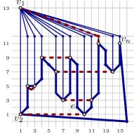
Figure 10: A RacSefe drawing of a wheel (solid; its rim is drawn in bold) and a matching (dashed)

We first compute the $x$-coordinates of the vertices. We do this such that $\mathcal{C}-\{(v_{n},v_{2})\}$ is $x$-monotone; see Figure 10. More precisely, for $i\in\{2,\ldots,n\}$, we set $x(v_{i})=2i-3$. The $y$-coordinates of the vertices are computed based on the matching $\mathcal{M}^{\prime}$ as follows. Let $E_{\mathcal{M}^{\prime}}=\{e_{1},\ldots,e_{k}\}$ be the matching edges, indexed such that $v_{2}$ is incident to $e_{1}$. For $j\in\{1,\ldots,k\}$, we assign the $y$-coordinate $2j-1$ to the endpoints of $e_{j}$. Next, we assign the $y$-coordinate $2k+1$ to the vertices incident to the rim without a matching edge in $\mathcal{M}^{\prime}$. Finally, the hub $v_{1}$ of $\mathcal{W}$ is located at point $(1,2k+3)$.

It remains to place the bend of each edge $e\in E_{\mathcal{W}}$; the edges in $\mathcal{M}^{\prime}$ are drawn without bends. First, let $e=(v_{1},v_{i})$, $i\in\{3,\ldots,n\}$ be a spike. Then, we place the bend at $(x(v_{i}),2k+2)$. Since both $v_{1}$ and $v_{2}$ are located in column 1, we can save the bend of the spike $(v_{1},v_{2})$. Second, let $e=(v_{i},v_{i+1})$, $i\in\{2,\ldots,n-1\}$ be an edge of the rim $\mathcal{C}$. We place the bend according to the following case distinction.

1. If $y(v_{i+1})>y(v_{i})$, we place the bend at $(x(v_{i+1}),y(v_{i})+1)$.

2. If $y(v_{i-1})>y(v_{i})>y(v_{i+1})$, we place the bend at $(x(v_{i+1}),y(v_{i})-1)$.

3. If $y(v_{i})>\max\{y(v_{i-1}),y(v_{i+1})\}$, by (i) the bottom port at $v_{i}$ is already used; see the edge $e$ in Figure 10. Thus, we draw $e$ with two bends; at $(x(v_{i})+1,y(v_{i})-1)$ and $(x(v_{i})+1,y(v_{i+1})+1)$.

Now, let $e=(v_{n},v_{2})$ be the remaining edge of the rim. We place its bend at $(2n-2,0)$.

Our approach ensures that $\mathcal{C}-\{(v_{n},v_{2})\}$ is drawn $x$-monotone, hence planar. The last edge $(v_{n},v_{2})$ of $\mathcal{C}$ is the only edge drawn outside of the bounding box that contains all vertices. Therefore, also the last edge is crossing-free. The spikes are not involved in crossings with the rim, as they are outside of the bounding box containing the rim edges. Hence, the drawing of $\mathcal{W}$ is planar. All edges of $\mathcal{M}^{\prime}$ are drawn as horizontal, non-overlapping line segments, so $\mathcal{M}^{\prime}$ is drawn planar as well. The slanted segments of $\mathcal{W}-{(v_{n},v_{2})}$ are of $y$-length 1, so they cannot be crossed by the edges of $\mathcal{M}^{\prime}$. As the edge $(v_{n},v_{2})$ is not involved in crossings, it follows that all crossings between $\mathcal{W}$ and $\mathcal{M}^{\prime}$ form right angles.

Finally, we have to insert the matching edge $(v_{1},v_{i})$ incident to the hub. Note that this edge also exists in $\mathcal{W}$ as a spike. Since $v_{i}$ is not incident to a matching edge in $\mathcal{M}^{\prime}$, it is placed above all matching edges. Therefore, the copy of $(v_{1},v_{i})$ in $\mathcal{W}$ does not cross a matching edge, and we can use the same layout for the copy of $(v_{1},v_{i})$ in $\mathcal{M}$.

We now show that our algorithm supports the Sefe model. Suppose that there is an edge $e=(v,v^{\prime})$ that belongs to both the rim $\mathcal{C}$ and the matching $\mathcal{M}$. If $e$ is the closing edge of the rim, then it is drawn planar in $\mathcal{C}$. Thus, this drawing can be used for both graphs. Otherwise, our algorithm places $v$ and $v^{\prime}$ at consecutive $x$-coordinates and at the same $y$-coordinate. Then, we can draw $e$ as a horizontal edge of length 1 in both graphs, and such an edge cannot be crossed.

We now prove the area bound of the drawing algorithm. To that end, we remove all columns that contain neither a vertex, nor a bend. First, we count the rows used. Since we remove the matching edge incident to $v_{1}$, the matching $\mathcal{M}^{\prime}$ has $k\leq n/2-1$ matching edges. We place the bottommost vertex in row $1$ and the topmost vertex (that is, vertex $v_{1}$) in row $2k+3$. We add one extra bend in row $0$ for the edge $(v_{n},v_{2})$. Thus, our drawing uses $2k+3+1\leq n+2$ rows. Next, we count the columns used. The vertices $v_{2},\dots,v_{n}$ are each placed in their own column. Every spike has exactly one bend in the column of a vertex. An edge $(v_{i},v_{i+1})$ of rim $\mathcal{W}$ has exactly one bend in a vertex column, except for the case that $y(v_{i})>y(v_{i-1}),y(v_{i+1})$. In this case it needs an extra bend between $v_{i}$ and $v_{i+1}$, $i=1,\ldots,n-1$. Clearly, there can be at most $n/2-1$ vertices satisfying this condition. Since the edge $(v_{n},v_{2})$ uses an extra column to the right of $v_{n}$, our drawing uses $(n-1)+(n/2-1)+1=1.5n-1$ columns.

(a) A non-planar drawing

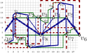
(b) A RacSefe drawing

Figure 11: Two drawings of the same outerpath and matching. In both figures, the outerpath is drawn solid, the upper and the lower path are drawn in bold, the spine of the spanning caterpillar is drawn extra bold and the matching is drawn dashed.

Theorem 4.2

An outerpath and a matching on a common set of $n$ vertices admit a RacSefe drawing on an integer grid of size $(3n-2)\times(2n-1)$ with two bends per outerpath edge and one bend per matching edge. The drawing can be computed in $O(n\log n)$ time.

Proof

Let $\mathcal{Z}=(V,E_{\mathcal{Z}})$ be the given outerpath and $\mathcal{M}=(V,E_{\mathcal{M}})$ the given matching. Recall that an outerpath is a biconnected outerplanar graph whose weak dual is a path of length at least two; see Figure 11(a). Furthermore, assume initially that $\mathcal{Z}$ and $\mathcal{M}$ do not share edges. Let $V=\{v_{1},v_{2},\ldots,v_{n}\}$, indexed such that $\langle v_{1},v_{2},\ldots,v_{n},v_{1}\rangle$ is the outer face of $\mathcal{Z}$.

We start by augmenting $\mathcal{Z}$ to a maximal outerpath $\mathcal{Z}^{\prime}=(V,E_{\mathcal{Z}^{\prime}})$ by triangulating its bounded faces. As $\mathcal{Z}^{\prime}$ is internally-triangulated, it contains exactly two vertices of degree two, each of which lies on a face that is an endpoint of the dual path. We assume, without loss of generality, that $\deg(v_{n})=\deg(v_{j})=2$ for some $j$ with $1<j<n$; see $v_{10}$ and $v_{6}$ in Figure 11(a). We call the path $\mathcal{P}_{\mathrm{u}}=(V_{\mathrm{u}},E_{\mathrm{u}})=\langle v_{1},v_{2},\ldots,v_{j-1}\rangle$ the upper path of $\mathcal{Z}^{\prime}$, and $\mathcal{P}_{\mathrm{l}}=(V_{\mathrm{l}},E_{\mathrm{l}})=\langle v_{j},v_{j+1},\ldots,v_{n}\rangle$ the lower path of $\mathcal{Z}^{\prime}$. Observe that $V=V_{\mathrm{u}}\cup V_{\mathrm{l}}$. If we remove $E_{\mathrm{u}}\cup E_{\mathrm{l}}$ from $E_{\mathcal{Z}^{\prime}}$, then the resulting graph is a caterpillar $\mathcal{C}$ that spans $V$ and whose spine alternates between vertices of $V_{\mathrm{u}}$ and $V_{\mathrm{l}}$.

We first compute the left-to-right order of the vertices of caterpillar $\mathcal{C}=(V_{\mathcal{C}},E_{\mathcal{C}})$ as described by the algorithm supporting Theorem 3.2. Then, the $x$-coordinate of the $i$^th vertex in this order is $3i-2$, $i=1,2,\ldots,n$; see Figure 11(b).

In order to compute the $y$-coordinates of the vertices, we first partition $\mathcal{M}$ into three matchings $\mathcal{M}_{\mathrm{ll}}=(V_{\mathrm{ll}},E_{\mathrm{ll}})$, $\mathcal{M}_{\mathrm{uu}}=(V_{\mathrm{uu}},E_{\mathrm{uu}})$ and $\mathcal{M}_{\mathrm{ul}}=(V_{\mathrm{ul}},E_{\mathrm{ul}})$ as follows. Let $(v,v^{\prime})\in E_{\mathcal{M}}$. Then,

1. $(v,v^{\prime})\in E_{\mathrm{ll}}$ if $v,v^{\prime}\in V_{\mathrm{l}}$,

2. $(v,v^{\prime})\in E_{\mathrm{uu}}$ if $v,v^{\prime}\in V_{\mathrm{u}}$,

3. $(v,v^{\prime})\in E_{\mathrm{ul}}$ if $v\in V_{\mathrm{u}}$ and $v^{\prime}\in V_{\mathrm{l}}$.

Since $V=V_{\mathrm{u}}\cup V_{\mathrm{l}}$, it holds that $E_{\mathcal{M}}=E_{\mathrm{ll}}\cup E_{\mathrm{uu}}\cup E_{\mathrm{ul}}$. In the resulting layout, the edges in $E_{\mathrm{ll}}$ will be drawn below the edges in $E_{\mathrm{ul}}$, which in turn will be drawn below the ones of $E_{\mathrm{uu}}$; see Figure 11(b). Thus, they will not cross each other.

Let $m_{\mathrm{ll}}=|E_{\mathrm{ll}}|$ and $E_{\mathrm{ll}}=\{e_{1},\ldots,e_{m_{\mathrm{ll}}}\}$. We draw the edges from bottom to top, starting from row 1. For $i=1,\ldots,m_{\mathrm{ll}}$, let $e_{i}=(u_{i},u_{i}^{\prime})$ with $x(u_{i})<x(u_{i}^{\prime})$. We set $y(u_{i})=4i-1$ and $y(u_{i}^{\prime})=4i-3$. Edge $e_{i}$ is drawn with a bend at $(x(u_{i}),y(u_{i}^{\prime}))$. Our approach ensures that there are no crossings between edges of $\mathcal{M}_{\mathrm{ll}}$, as they are drawn in different horizontal strips of the drawing. Similarly, we draw the edges in $E_{\mathrm{uu}}$ from top to bottom, starting from row $2n-1$. Let $m_{\mathrm{uu}}=|E_{\mathrm{uu}}|$. By construction, the topmost vertex of $V_{\mathrm{ll}}$ is drawn in the row $4m_{\mathrm{ll}}-1$ and the bottommost vertex of $V_{\mathrm{uu}}$ is drawn in the row $2n+1-4m_{\mathrm{uu}}$. The vertices of $V_{\mathrm{ul}}$ will be drawn between these rows; see Figure 11(b).

In order to draw the edges in $E_{\mathrm{ul}}$, we process the vertices of the set $V_{\mathrm{ul}}$ from left to right and assign $y$-coordinates to both endpoints of the incident matching edge. Let $m_{\mathrm{ul}}=|E_{\mathrm{ul}}|$ and $E_{\mathrm{ul}}=\{\hat{e}_{1},\ldots,\hat{e}_{m_{\mathrm{ul}}}\}$. For $k\in\{1,\ldots,\mu\}$, let $\hat{e}_{k}=(w_{k},w_{k}^{\prime})$ and assume without loss of generality that $x(w_{k})<x(w_{k}^{\prime})$ and $x(w_{1})<\ldots<x(w_{\mu})$. We place the vertices in $V_{\mathrm{l}}$ from bottom to top and the vertices in $V_{\mathrm{u}}\cap V_{\mathrm{ul}}$ from top to bottom. If $w_{k}\in V_{\mathrm{u}}$, we assign the $y$-coordinate $4m_{\mathrm{ll}}-1+3k$ to $w_{k}$ and the $y$-coordinate $2n+1-4m_{\mathrm{uu}}$ to $w_{k}^{\prime}$; if $w_{k}\in V_{\mathrm{l}}$, we switch the $y$-coordinates. Edge $\hat{e}_{k}$ is drawn with a bend at $(x(w_{k}),y(w_{k}^{\prime}))$. Further, every edge $\hat{e}_{l}\in E_{\mathrm{ul}}$ with $l>k$ has its endpoints to the right of $w_{k}$ and in the horizontal strip defined by the lines $y=y(w_{k})$ and $y=y(w_{k}^{\prime})$. Hence, it will not be involved in crossings with $(w_{k},w_{k}^{\prime})$. This guarantees that the drawing of $\mathcal{M}$ is planar.

It remains to determine, for each edge $e=(v,v^{\prime})\in\mathcal{Z}^{\prime}$, where to place its bend. Without loss of generality, let $e$ be directed from its left endpoint, say $v$, to its right endpoint, say $v^{\prime}$. First, assume that $e\in E_{\mathrm{u}}\cup E_{\mathrm{l}}$ belongs to the outercycle. Then, we place its bends at $(x(v^{\prime})-2,y(v))$ and $(x(v^{\prime})-2,y(v^{\prime})-\operatorname{sgn}(y(v^{\prime})-y(v)))$. Second, assume that $e\in E_{\mathcal{C}}$ belongs to the inner caterpillar. Then, we place its bends at $(x(v^{\prime})-1,y(v)+\operatorname{sgn}(y(v)-y(v^{\prime})))$ and $(x(v^{\prime})-1,y(v^{\prime})-\operatorname{sgn}(y(v^{\prime})-y(v)))$.

Since $\mathcal{P}_{\mathrm{u}}$ and $\mathcal{P}_{\mathrm{l}}$ are drawn $x$-monotone, both are drawn planar. Following similar arguments as in the proof of Theorem 3.2, we can show that $\mathcal{C}$ is drawn planar as well. Since $\mathcal{C}$ is drawn between $\mathcal{P}_{\mathrm{u}}$ and $\mathcal{P}_{\mathrm{l}}$, it follows that $\mathcal{Z}^{\prime}$ is drawn planar, as desired. It now remains to prove that all (potential) crossings between $\mathcal{Z}^{\prime}$ and $\mathcal{M}$ only involve rectilinear edge segments of $\mathcal{Z}^{\prime}$, as $\mathcal{M}$ consists exclusively of rectilinear segments. As all slanted segments of $\mathcal{Z}^{\prime}$ are of $y$-length 1, no horizontal segment of $\mathcal{M}$ can cross them. The same holds for vertical segments of $\mathcal{M}_{\mathrm{uu}}\cup\mathcal{M}_{\mathrm{ll}}$, as they are drawn above and below $\mathcal{P}_{\mathrm{l}}$ and $\mathcal{P}_{\mathrm{u}}$, respectively. The only possible non-rectilinear crossings are between a vertical segment of a matching edge $(u,v)\in E_{\mathrm{ul}}$ and a long slanted segment of $\mathcal{C}$ incident to a spine vertex $w$. This crossing can only occur if $w$ lies to the left of the vertical segment of $(u,v)$. By construction, $w$ is never drawn between $u$ and $v$, with respect to the $y$-coordinate. Thus, such crossings cannot occur, which implies all crossings between $\mathcal{Z}^{\prime}$ and $\mathcal{M}$ form right angles.

We now show that our algorithm supports the Sefe model. Assume that $\mathcal{M}$ and $\mathcal{Z}$ share edges, and let $e=(v,v^{\prime})$ be an edge that belongs to both input graphs. If $e\in E_{\mathrm{l}}$, then also $e\in E_{\mathrm{ll}}$. Our algorithm places $v$ and $v^{\prime}$ at consecutive $y$-coordinates and determines their $x$-coordinates such that no other vertex of $V_{\mathrm{l}}$ lies between them. Thus, edge $e$ is drawn in the matching as a vertical segment of length 2 and a horizontal segment that has no vertex below it. Hence, the drawing of $e$ in the matching is planar and can be used for both graphs. The case $e\in E_{\mathrm{u}}$ is analogous.

If $e\in E_{\mathcal{C}}$, then also $e\in E_{\mathrm{ul}}$. In this case, we observe that the topological routing of $e$ is the same in both graphs with an offset of one unit to avoid overlaps. Thus, every other edge either crosses both or none of the drawings of $e$. Since each drawing of $e$ forbids crossings by edges of one of the input graphs, actually none of the two drawings can have a crossing. Hence, we can draw $e$ the same way in both graphs.

By the choice of the coordinates, the area requirement of our algorithm is $(3n-2)\times(2n-1)$. Since we have to sort the edges in $E_{\mathrm{ul}}$ by the $x$-coordinates of the incident vertices, our algorithm runs in $O(n\log n)$ time. To complete the proof of this theorem, observe that the extra edges that we introduced when augmenting $\mathcal{Z}$ to $\mathcal{Z}^{\prime}$ can be safely removed from the constructed layout, affecting neither the crossing angles nor the area of the layout.

5 Conclusions and Open Problems

In this paper, we have studied RacSefe and RacSim drawings with few bends per edge. We have proven that two planar graphs always admit a RacSim drawing with at most six bends per edge. For more restricted classes of graphs, we have reduced the number of bends per edge. Some of these specialized results also hold for the stronger RacSefe model. All drawings of our algorithms fit it quadratic area.

Our results raise several questions that remain open. First of all, can we strengthen any of our results from RacSim to RacSefe (see Table 1); for example, for a pair of general planar graphs? For the classes of graphs that we have presented in this paper, can we reduce the number of bends per edge or can we show lower bounds? Are there other graph classes that admit RacSim drawings with few bends? Can we reduce the number of bends per edge by relaxing the strict constraint that edge intersections are at right angles and instead ask for drawings that have close to optimal crossing resolution? What about the computational complexity of the general problem, that is, given two or more planar graphs on the same set of vertices and a non-negative integer $k$, can we decide efficiently whether there is a RacSim drawing in which each graph is drawn with at most $k$ bends per edge and the crossings are all at right angles? This seems unlikely. Finally, is it possible to achieve sub-quadratic area for RacSim drawings of subclasses of planar graphs when accepting more bends per edge?

References

- [1] P. Angelini, G. D. Battista, F. Frati, M. Patrignani, and I. Rutter. Testing the simultaneous embeddability of two graphs whose intersection is a biconnected or a connected graph. J. Discrete Algorithms, 14:150–172, 2012. doi:10.1007/978-3-642-19222-7_22.
- [2] P. Angelini, G. Di Battista, F. Frati, V. Jelínek, J. Kratochvíl, M. Patrignani, and I. Rutter. Testing planarity of partially embedded graphs. ACM Trans. Algorithms, 11(4):32:1–32:42, 2015. doi:10.1145/2629341.
- [3] P. Angelini, M. Geyer, M. Kaufmann, and D. Neuwirth. On a tree and a path with no geometric simultaneous embedding. J. Graph Algorithms Appl., 16(1):37–83, 2012. doi:10.1.1.278.6159.
- [4] E. N. Argyriou, M. A. Bekos, M. Kaufmann, and A. Symvonis. Geometric RAC simultaneous drawings of graphs. J. Graph Algorithms Appl., 17(1):11–34, 2013. doi:10.7155/jgaa.00282.
- [5] M. A. Bekos, M. Gronemann, and Ch. N. Raftopoulou. Two-page book embeddings of 4-planar graphs. In E. W. Mayr and N. Portier, editors, 31st Int. Symp. Theor. Aspects Comput. Sci. (STACS’14), volume 25 of LIPIcs, pages 137–148. Schloss Dagstuhl – Leibniz-Zentrum für Informatik, 2014. doi:10.4230/LIPIcs.STACS.2014.137.
- [6] F. Bernhart and P. C. Kainen. The book thickness of a graph. J. Comb. Theory, Series B, 27(3):320–331, 1979. doi:10.1016/0095-8956(79)90021-2.
- [7] T. Bläsius, A. Karrer, and I. Rutter. Simultaneous embedding: Edge orderings, relative positions, cutvertices. In S. Wismath and A. Wolff, editors, Proc. 21st Int. Symp. Graph Drawing (GD’13), volume 8242 of LNCS, pages 220–231. Springer-Verlag, 2013. doi:10.1007/978-3-319-03841-4_20.
- [8] T. Bläsius, S. G. Kobourov, and I. Rutter. Simultaneous embedding of planar graphs. In R. Tamassia, editor, Handbook of Graph Drawing and Visualization, chapter 11, pages 349–381. CRC Press, 2013. URL: http://www.crcpress.com/product/isbn/9781584884125.
- [9] P. Brass, E. Cenek, C. A. Duncan, A. Efrat, C. Erten, D. P. Ismailescu, S. G. Kobourov, A. Lubiw, and J. S. Mitchell. On simultaneous planar graph embeddings. Comput. Geom. Theory Appl., 36(2):117–130, 2007. doi:10.1016/j.comgeo.2006.05.006.
- [10] G. Brightwell and E. R. Scheinerman. Representations of planar graphs. SIAM J. Discrete Math., 6(2):214–229, 1993. doi:10.1137/0406017.
- [11] S. Cabello, M. van Kreveld, G. Liotta, H. Meijer, B. Speckmann, and K. Verbeek. Geometric simultaneous embeddings of a graph and a matching. J. Graph Algorithms Appl., 15(1):79–96, 2011. doi:10.7155/jgaa.00218.
- [12] T. M. Chan, F. Frati, C. Gutwenger, A. Lubiw, P. Mutzel, and M. Schaefer. Minimum length embedding of planar graphs at fixed vertex locations. In C. A. Duncan and A. Symvonis, editors, Proc. 22nd Int. Symp. Graph Drawing (GD’14), volume 8871 of LNCS, pages 25–39. Springer-Verlag, 2014. Long version available at http://arxiv.org/abs/1410.8205. doi:10.1007/978-3-319-03841-4_33.
- [13] G. Cornuéjols, D. Naddef, and W. Pulleyblank. Halin graphs and the travelling salesman problem. Math. Program., 26(3):287–294, 1983. doi:10.1007/BF02591867.
- [14] E. Di Giacomo, W. Didimo, M. van Kreveld, G. Liotta, and B. Speckmann. Matched drawings of planar graphs. J. Graph Algorithms Appl., 13(3):423–445, 2009. doi:10.7155/jgaa.00193.
- [15] C. Erten and S. G. Kobourov. Simultaneous embedding of a planar graph and its dual on the grid. Theory Comput. Syst., 38(3):313–327, 2005. doi:10.1007/3-540-36136-7_50.
- [16] C. Erten and S. G. Kobourov. Simultaneous embedding of planar graphs with few bends. J. Graph Algorithms Appl., 9(3):347–364, 2005. doi:10.7155/jgaa.00113.
- [17] A. Estrella-Balderrama, E. Gassner, M. Jünger, M. Percan, M. Schaefer, and M. Schulz. Simultaneous geometric graph embeddings. In S.-H. Hong, T. Nishizeki, and W. Quan, editors, Proc. 15th Int. Symp. Graph Drawing (GD’07), volume 4875 of LNCS, pages 280–290. Springer-Verlag, 2008. doi:10.1007/978-3-540-77537-9_28.
- [18] S. Felsner. Geometric Graphs and Arrangements. Vieweg Verlag, 2004. doi:10.1007/978-3-322-80303-0.
- [19] F. Frati, M. Hoffmann, and V. Kusters. Simultanteous embeddings with few bends and crossings. In E. Di Giacomo and A. Lubiw, editors, Proc. 23rd Int. Symp. Graph Drawing (GD’15), volume 9411 of LNCS, pages 166–179. Springer-Verlag, 2015. doi:10.1007/978-3-319-27261-0_14.
- [20] L. Grilli, S.-H. Hong, J. Kratochvíl, and I. Rutter. Drawing simultaneously embedded graphs with few bends. In C. Duncan and A. Symvonis, editors, Proc. 22nd Int. Symp. Graph Drawing (GD’14), volume 8871 of LNCS, pages 40–51. Springer-Verlag, 2014. doi:10.1007/978-3-662-45803-7_4.
- [21] B. Haeupler, K. R. Jampani, and A. Lubiw. Testing simultaneous planarity when the common graph is 2-connected. J. Graph Algorithms Appl., 17(3):147–171, 2013. doi:10.7155/jgaa.00289.
- [22] Ch. Haslinger and P. F. Stadler. RNA structures with pseudo-knots: Graph-theoretical, combinatorial, and statistical properties. Bull. Math. Biol., 61(3):437–467, 1999. doi:10.1006/bulm.1998.0085.
- [23] L. Heath. Embedding outerplanar graphs in small books. SIAM J. Algebr. Discrete Meth., 8(2):198–218, 1987. doi:10.1137/0608018.
- [24] L. S. Heath. Algorithms for Embedding Graphs in Books. PhD thesis, University of North Carolina, Chapel Hill, 1985. URL: http://www.cs.unc.edu/techreports/85-028.pdf.
- [25] P. C. Kainen and S. Overbay. Extension of a theorem of Whitney. Appl. Math. Lett., 20(7):835–837, 2007. doi:10.1016/j.aml.2006.08.019.
- [26] F. Kammer. Simultaneous embedding with two bends per edge in polynomial area. In L. Arge and R. Freivalds, editors, Proc. 10th Scand. Workshop Algorithm Theory (SWAT’06), volume 4059 of LNCS, pages 255–267. Springer-Verlag, 2006. doi:10.1007/11785293_25.
- [27] M. Kaufmann and R. Wiese. Embedding vertices at points: Few bends suffice for planar graphs. J. Graph Algorithms Appl., 6(1):115–129, 2002. doi:10.7155/jgaa.00046.
- [28] C. St. J. A. Nash-Williams. Decomposition of finite graphs into forests. J. London Math. Soc., 39(1):12, 1964. doi:10.1112/jlms/s1-39.1.12.
- [29] T. Nishizeki and N. Chiba. Planar Graphs: Theory and Algorithms, chapter Chapter 10. Hamiltonian Cycles, pages 171–184. Dover Books Math. Courier Dover Pub., 2008. URL: http://store.doverpublications.com/048646671x.html.
- [30] M. Schaefer. Toward a theory of planarity: Hanani-Tutte and planarity variants. J. Graph Algorithms Appl., 17(4):367–440, 2013. doi:10.7155/jgaa.00298.
- [31] A. Wigderson. The complexity of the Hamiltonian circuit problem for maximal planar graphs. Technical Report TR-298, EECS Department, Princeton University, 1982. URL: http://www.math.ias.edu/~avi/PUBLICATIONS/MYPAPERS/W82a/tech298.pdf.