Design and performance of coded aperture optical elements
for the CESR-TA x-ray beam size monitor

Abstract

We describe the design and performance of optical elements for an x-ray beam size monitor (xBSM), a device measuring $e^{+}$ and $e^{-}$ beam sizes in the CESR-TA storage ring. The device can measure vertical beam sizes of $10-100~{}\mu$m on a turn-by-turn, bunch-by-bunch basis at $e^{\pm}$ beam energies of $\sim 2-5~{}$GeV. X-rays produced by a hard-bend magnet pass through a single- or multiple-slit (coded aperture) optical element onto a detector. The coded aperture slit pattern and thickness of masking material forming that pattern can both be tuned for optimal resolving power. We describe several such optical elements and show how well predictions of simple models track measured performances.

1 Introduction

Precision measurement of vertical bunch size plays an increasingly important role in the design and operation of the current and future generation of electron storage rings. By providing the operator with real-time vertical beam size information, the accelerator can be tuned in a predictable, stable, and robust manner. Challenges persist in obtaining adequate precision at small beam size, low beam energy, and/or low beam current. The CESR-TA x-ray beam size monitor [1, 2, 3, 4, 5, 6, 7, 8, 9, 10, 11, 12, 13] (xBSM) images synchrotron radiation from a hard-bend magnet through a single- or multi-slit optical element onto a 32-strip photodiode detector with 50  ${\mu\mathrm{m}}$ pitch and sub-ns response. Here we extend the characterization of that device, focusing on comparing measured with predicted resolving power for each of several different optical elements. To the extent that a prediction matches measurements, one can gain confidence that the associated model can be used to optimize optical element design in other specific situations.

A simplified schematic of the CESR-TA xBSM setup is shown in Fig. 1, with relevant dimensions in Table 1. Separate installations exist for electrons and positrons.

Ref. [13] describes our use of both single-slit (pinhole) and multi-slit optical elements, the latter of which are known as coded apertures. Coded aperture imaging [14] can, in principle, improve upon the spatial resolution of a pinhole camera. This can be achieved by having greater x-ray intensity at the image (due to more open area at the optic), carefully designed slit sizes and spacings, and a well-tuned thickness of the semi-opaque masking material between the slits. An optimized mask may be thin enough to partially transmit x-rays with a phase shift. Through interference, light passing through the slits and mask will affect the point response function (prf) [13] for good or ill, depending on the coded aperture pattern, mask thickness, and x-ray spectrum. Our coded apertures use a gold masking material of 0.5-0.8 ${\mu\mathrm{m}}$ thickness on top of a 2.5 ${\mu\mathrm{m}}$-thick silicon substrate (which also absorbs x-rays, but does so identically for both slit and mask regions). Masking of an intermediate thickness can be more effective than a thicker choice because it introduces a significant phase shift while preserving a larger fraction of the incident intensity for distribution among the peaks and valleys of the prf. As with the pattern of slits, masking thickness and associated cooling must be chosen to balance improved beam size sensitivity in the prf against decreased susceptibility to radiation damage.

Optical elements used at CESR-TA are listed in Table 2, and include wide-open (WO), an adjustable vertical pinhole (PH), and two coded aperture designs (CA1 and CA2). Our coded apertures were acquired from Applied Nanotools, Inc. [15], and are created with a proprietary process which lays out a patterned gold masking layer on a 2.5 ${\mu\mathrm{m}}$-thick silicon substrate chip. The two coded aperture designs that we have used appear in high resolution photographs in Fig. 2, and have parameters summarized in Table 2. Optical measurements indicate that the systematic placement of features is within 0.5 ${\mu\mathrm{m}}$ of the specifications. Edge quality is better than 0.1 ${\mu\mathrm{m}}$ rms deviation.

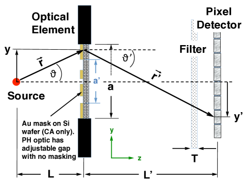
Figure 1: Simplified schematic of xBSM layout (not to scale). The distinction between $a$ and ${a^{\,\prime}}$ is that $a$ is the total vertical extent of partial transmission through the mask material, and ${a^{\,\prime}}$ is the vertical extent of features (slits) in the mask.

Table 1: Geometrical parameters defining the CESR-TA xBSM beamlines. Geometrical quantities are defined in Fig. 1. Distances assume the coded aperture optic; the pinhole optic is 25 ${\mathrm{mm}}$ closer to the source point and hence has a magnification value about 1% larger than shown. The uncertainties on $L$ are from an optical survey. The uncertainties on ${L^{\,\prime}}$ are from the survey, CESR orbit, and the associated depth of field.

Parameter	$e^{-}$ beamline	$e^{+}$ beamline
$L$	$4356.5\pm 3.9$ ${\mathrm{mm}}$	$4485.2\pm 4.0$ ${\mathrm{mm}}$
${L^{\,\prime}}$	$10621.1\pm 1.0$ ${\mathrm{mm}}$	$10011.7\pm 1.0$ ${\mathrm{mm}}$
$M\equiv{L^{\,\prime}}/L$	$2.4380\pm 0.0022$	$2.2322\pm 0.0020$
${a^{\,\prime}}$	$\approx 50-300$ ${\mu\mathrm{m}}$	same as $e^{-}$
$a$	$\approx 50-1000$ ${\mu\mathrm{m}}$	same as $e^{-}$
$2\theta_{\rm max}={a^{\,\prime}}/L$	$11-69~{}\mu$rad	$11-67~{}\mu$rad

Table 2: CESR-TA xBSM optic element parameters. Geometrical quantities are defined in Fig. 1. Coded aperture patterns are shown in Fig. 2.

Category	Parameter	Value
WO	${a^{\,\prime}}\equiv a$	40 mm
(wide-open)
PH	Tungsten blade $T$	2.5 ${\mathrm{mm}}$
(pinhole)	Downstream taper	$2^{\circ}$
	$a$	0-200 ${\mu\mathrm{m}}$
	${a^{\,\prime}}$	$\equiv a$
CA1	Si $T$	2.5 ${\mu\mathrm{m}}$
(coded	Au $T$ (2 chips)	$0.54\pm 0.05$ ${\mu\mathrm{m}}$
aperture)	Au $T$ (2 chips)	$0.69\pm 0.05$ ${\mu\mathrm{m}}$
	Au $T$ (1 chip)	$0.75\pm 0.05$ ${\mu\mathrm{m}}$
	$a$	1000 ${\mu\mathrm{m}}$
	${a^{\,\prime}}$	280 ${\mu\mathrm{m}}$
	# slits	8
	Min/Max slit width	10/40 ${\mu\mathrm{m}}$
	Transmitting fraction of ${a^{\,\prime}}$	54%
	Feature placement accuracy	0.5 ${\mu\mathrm{m}}$
	Edge quality rms deviation	0.1 ${\mu\mathrm{m}}$
	Pattern: S=slit, M=mask ($\mu$m)
	20S-10M-20S-10M-40S-
	30M-10S-10M-10S-10M-
	30S-40M-10S-20M-10S
CA2	Si $T$	2.5 ${\mu\mathrm{m}}$
	Au $T$	$0.62\pm 0.05$ ${\mu\mathrm{m}}$
	Au $T$	$0.75\pm 0.05$ ${\mu\mathrm{m}}$
	$a$	1000 ${\mu\mathrm{m}}$
	${a^{\,\prime}}$	296 ${\mu\mathrm{m}}$
	# slits	5
	Min/Max slit width	10/68 ${\mu\mathrm{m}}$
	Transmitting fraction of ${a^{\,\prime}}$	65%
	Feature placement accuracy	0.5 ${\mu\mathrm{m}}$
	Edge quality rms deviation	0.1 ${\mu\mathrm{m}}$
	Pattern: S=slit, M=mask ($\mu$m)
	24S-10M-38S-42M-68S-
	42M-38S-10M-24S

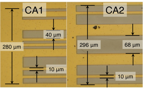
Figure 2: Photographs of portions of CESR-TA xBSM coded aperture optical elements CA1 (left) and CA2 (right).Dark strips indicate transmission slits, while lighter areas represent the gold coating. The imperfections (black spots) are remnants of etching resist with thickness $\sim$0.01 ${\mu\mathrm{m}}$, which are essentially transparent to x-rays.

2 Resolving Power

Design and quantitative evaluation of optical elements requires a figure of merit for beam size determination. The goal in optic design is to obtain the broadest possible regions of beam size where the figure of merit for a particular design is larger than the alternatives in the relevant ranges of beam size and current. For sufficiently large current, the figure of merit should approach being current-independent; however, its usefulness is at low current, where significant current dependence remains. The regime for which it is most difficult to obtain adequate sensitivity is that of simultaneous small beam size and low beam current.

In Eq. (16) of Ref. [13] we restricted ourselves to an idealized figure of merit wherein effects from fitting for the beam size and other parameters on a turn-by-turn basis were ignored. The resulting function $\mathcal{Q}({\sigma_{b}})$ expressing a simplified statistical power of a particular optical element at beam size ${\sigma_{b}}$. $\mathcal{Q}({\sigma_{b}})$ is a $\chi^{2}$-like quantity based on the assertion that the pulse height in each of the 32 pixels is proportional to the number of incident photons depositing energy there and which will fluctuate according to Gaussian counting statistics. The $\mathcal{P}_{0}$ term present in that formula represents the electronic pedestal noise, the rms variation in each channel’s pulse height when no charge has been deposited. $\mathcal{P}_{0}$ introduces an explicit beam current dependence to the prediction because its size relative to peak values will change with current. A reasonable parameterizaton is $\mathcal{P}_{0}(I)=p_{0}/I$, with the current-independent parameter $p_{0}$ determined from experiment. With this modification, we rewrite Eq. (16) of Ref. [13] as follows, an initial prediction we refer to as “model 1”:

$$\mathcal{Q}_{P1}({\sigma_{b}},I) \equiv\mathcal{Q}_{0}\;\left(\dfrac{{\sigma_{b}}}{\delta}\right)^{2}\times$$ (1)

$$\sum_{\rm pixels}\dfrac{\left[\mathcal{P}_{j}({\sigma_{b}})-\mathcal{P}_{j}({\sigma_{b}}+\delta)-\mathcal{D}({\sigma_{b}},\delta)\right]^{2}}{\mathcal{P}_{j}({\sigma_{b}})+\mathcal{P}_{j}({\sigma_{b}}+\delta)+2\,p_{0}/I}\,,$$

where $\mathcal{P}_{j}({\sigma_{b}})$ is the point response function integrated over pixel $j$, $\delta$ is an incremental change in beam size (we use $\delta=8$ ${\mu\mathrm{m}}$), $\mathcal{D}({\sigma_{b}},\delta)$ is the difference between the value of $\mathcal{P}_{j}({\sigma_{b}})$ averaged over all pixels ($j$) and the similarly averaged $\mathcal{P}_{j}({\sigma_{b}}+\delta)$, $I$ is the beam current, and $\mathcal{Q}_{0}$ is an overall normalization factor. For optical elements that keep the primary image features well-contained on the detector for modest beam sizes, $\mathcal{D}({\sigma_{b}},\delta)$ will be negligibly small; however, for very large beam sizes or optic designs with image features close to the detector edges, it can become significantly nonzero.

In order to extract a measured figure of merit from the data that we can compare with a prediction, we first re-arrange Eq. (17) of Ref. [13] as

$$\mathcal{Q}_{M}({\sigma_{b}},I,H)=\dfrac{10~{}\mu{\rm A}}{I}\;\dfrac{{\left<{\sigma_{b}}\right>}^{2}}{{\left<{(\Delta\sigma_{b})^{2}}\right>}}\;,$$ (2)

where ${\left<{\sigma_{b}}\right>}$ is the turn-averaged beam size, ${\left<{(\Delta\sigma_{b})^{2}}\right>}$ is its variance, $I$ is the beam current, and where we have introduced dependence upon the horizontal illumination $H$. $H$ affects ${\left<{(\Delta\sigma_{b})^{2}}\right>}$ through variations in light flux incident upon the detector per unit beam current. Different optical elements can (and do) have different widths of the horizontally limiting slit mounted just in front of the optic; different data runs can (and do) have different fractions of the active detector pixels properly aligned horizontally with the x-ray beam, as shown in Fig. 3. To remove dependence upon both $I$ and $H$ at which different datasets are acquired, we establish corrected quantities which bring any measured or predicted values to those expected from a fixed reference current $I_{0}$=0.25 mA and reference horizontal illumination $H_{0}$ for both predicted and measured quantities:

$$\mathcal{Q}_{Pj}^{\,\prime}({\sigma_{b}})\equiv\mathcal{Q}_{Pj}({\sigma_{b}},I_{0},H_{0})$$ (3)

and

$$\mathcal{Q}_{Mj}^{\,\prime}({\sigma_{b}})\equiv\mathcal{Q}_{M}({\sigma_{b}},I,H)\times\dfrac{\mathcal{Q}_{Pj}({\sigma_{b}},I_{0},H_{0})}{\mathcal{Q}_{Pj}({\sigma_{b}},I,H)}\,.$$ (4)

Without this correction, measured values taken at different currents or with different horizontally limiting slit widths or with different horizontal alignments could not be directly compared to each other or to model predictions. Note that $\mathcal{Q}_{Mj}^{\,\prime}({\sigma_{b}})$ depends upon a particular model $j$ because of the correction.

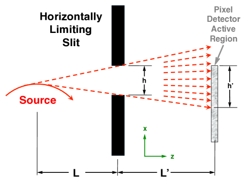
Figure 3: Simplified schematic (not to scale) of the xBSM layout, looking down onto the plane of the storage ring. The horizontally limiting slit just upstream of the optical element (not shown) has width $h$, and the portion of the pixel detector that is illuminated is $h^{\prime}$. In this example of sub-ideal alignment, a substantial fraction of the x-rays passing through the horizontally limiting slit (and subsequently through the optical element) miss the detector, resulting in an integrated pulse height smaller than would result with horizontal illumniation fully contained on the detector.

The horizontal illumination correction can be made by using the ratio $R$ of image area (integrated pulse height) per unit current to that for a specific optical element, filter, and beam energy defined as a reference. For any dataset, a deviation from unity in the measured ratio $R_{M}$ relative to the predicted one $R_{P}$ is taken as a proportional flux correction in the model prediction for that dataset by using current $I_{0}\times R_{P}/R_{M}$ instead of $I_{0}$.

As shall be seen in the following section, the simplified model embodied in $\mathcal{Q}_{P1}({\sigma_{b}},I)$ is far from adequate to accurately describe the data, most dramatically for the pinhole (PH) optic. This observation motivated the development of a second, more sophisticated, model $\mathcal{Q}_{P2}({\sigma_{b}},I,H)$ that includes four additional effects that the simple one does not: the Poisson (as opposed to Gaussian) photon-counting statistics that come into play for very small pulse heights, digitization, the fit of the image for each turn to a four-parameter function, and the $H$ correction. The predictions of model 2 are computed in a Monte Carlo simulation of 8k turns for each beam size on each turn using the following procedure:

1. Obtain the image shape function expected for the geometry, optical element, beam energy, and beam size in question (i.e., the function derived from the appropriate templates, as described in Sec. 2.3 of Ref. [13]).

2. Scale the resulting function so obtained so as to match the amplitude measured at the $I$ and $H$ applicable to that dataset.

3. Offset the function in the vertical direction by a different random amount so that the image centers span at least a full detector pixel (this corresponds to beam motion of about $\pm 10$ ${\mu\mathrm{m}}$).

4. Evaluate the function at all 32 pixel centers.

5. Smear each pixel pulse height, first with the Gaussian pedestal width and then with a Poisson distribution, using a fixed photon/adc conversion factor (see below).

6. Truncate the result to an integral number of adc counts to correctly reflect the digitization process.

7. Add a flat background that randomly varies turn-to-turn by the amount observed in the data; this component typically has a contribution which varies by up to $\pm$2% of the image area from one turn to another.

8. Subject the resulting image to the identical analysis software as used on the data so as to obtain a fitted beam size for each turn.

After analysis of all turns, a predicted ${\left<{\sigma_{b}}\right>}$ and ${\left<{(\Delta\sigma_{b})^{2}}\right>}$ are extracted, at which point the expression in Eq. (2) can be evaluated for this modeling of the figure of merit. This simulation is used to generate both beam size and current dependences of the figure of merit so that the data can be corrected to the reference current and horizontal illumination, resulting in a value for $\mathcal{Q}_{P2}^{\,\prime}({\sigma_{b}})$.

The factor setting the number of photons per adc count (used in step (v) above) is determined by matching measured turn-to-turn fluctuations in beam size, as embodied in the measured resolving power, to that obtained from model 2. However, once this is found for a given beam energy and optic at a single point of current and beam size, this same value is then applied to the other beam sizes and optical elements used at that beam energy. In the plots shown below, this calibration point is generally taken for a point near the smallest beam size that has the largest figure of merit. This one point is guaranteed to match the model, but all model predictions at other beam sizes and for other optical elements at that beam energy are not constrained to the measured $\mathcal{Q}_{M}({\sigma_{b}},I,H)$.

Table 3: Summary of datasets acquired for figure of merit measurements. All data were acquired with no filter in place except for the pinhole (PH) optic for 2.1 ${\mathrm{GeV}}$ positrons, where a diamond filter of thickness 4.4 ${\mu\mathrm{m}}$ was used. The fourth column specifies either the gold thickness for a coded aperture, or the gap size ${a^{\,\prime}}$ for a pinhole (PH). The quantity $A$ refers to the predicted total power incident upon the detector relative to that of the first row. The quantity $R_{M}/R_{P}$ describes the horizontal illumination relative to a reference dataset (see text). The $I$ column gives the current at which one or two datasets were acquired, and the last column gives the predicted figure of merit ${\cal{Q}}_{P2}^{\,\prime}$ evaluated at ${\sigma_{b}}$=15 ${\mu\mathrm{m}}$.

${E_{b}}$	$e^{\pm}$	Optic	Au or ${a^{\,\prime}}$	$A$	$R_{M}/R_{P}$	$I$	${\cal{Q}}_{P2}^{\,\prime}$
(GeV)		Optic	($\mu$m)	(rel)		(mA)	$(15~{}{\mu\mathrm{m}})$
1.8	$e^{+}$	CA2	0.75	1	1	0.85, 0.55	1.6
		CA1	0.75	0.83	1.00	0.73	0.57
		PH	53	0.53	0.99	1.00, 0.59	0.58
	$e^{-}$	CA2	0.60	1.13	0.77	0.88	1.76
		CA1	0.60	0.95	0.74	0.57	0.54
		CA1	0.71	0.87	0.41	0.49	0.55
		PH	54	0.56	0.35	0.43	0.67
2.1	$e^{-}$	CA2	0.60	5.04	0.77	0.43, 0.24	6.1
		CA1	0.60	4.26	0.81	0.57, 0.21	1.7
		CA1	0.71	3.82	0.56	0.81, 0.41	1.8
		PH	49	1.07	0.38	0.88, 0.41	2.3

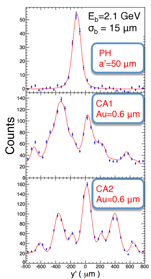
Figure 4: Detector images (points with error bars) taken at ${E_{b}}$=2.1 ${\mathrm{GeV}}$ using the PH (top), CA1 (middle), and CA2 (bottom) optical elements. The smooth curves show the best fits, which in all cases have ${\sigma_{b}}$$\approx$15 ${\mu\mathrm{m}}$.

3 Results

Data were acquired to measure optical element performance over a range of beam energies and beam sizes. A summary of these datasets appears in Table 3. For each dataset, the storage ring was filled with electrons or positrons, adjusted to a current below 1 mA, and several thousand turns were taken at each of a dozen or so beam sizes. For reference, single-turn images for all three optical elements taken with ${\sigma_{b}}$=15 ${\mu\mathrm{m}}$ at ${E_{b}}$=2.1 ${\mathrm{GeV}}$ appear in Fig. 4.

Results on optical element performance appear in Figs. 5-8. Note that model 1 does not predict the pinhole performance as accurately as model 2, emphasizing the importance of accounting for Poisson statistics and the more complete treatment of effects of the image fitting in model 2. Agreement between measurements and model 2 for coded apertures is reasonably good, especially below a beam size of 60 ${\mu\mathrm{m}}$. The measurements also verify that thinner gold masking performs better than thicker gold in a predictable manner.

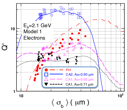
Figure 5: Comparison of the measured figures of merit $\mathcal{Q}_{Mj}^{\,\prime}({\sigma_{b}})$ (markers) for four optical elements (see text), with the corresponding predictions $\mathcal{Q}_{Pj}^{\,\prime}({\sigma_{b}})$ (curves) from model 1 for a ${E_{b}}=2.1$ ${\mathrm{GeV}}$ electron beam. Statistical uncertainties on the data points are smaller than the marker sizes.

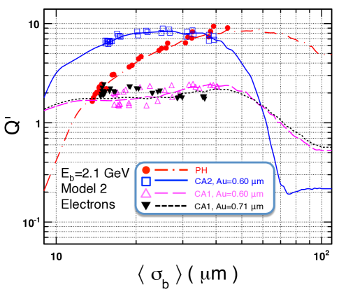
Figure 6: Comparison of the measured figures of merit $\mathcal{Q}_{Mj}^{\,\prime}({\sigma_{b}})$ (markers) for four optical elements (see text), with the corresponding predictions $\mathcal{Q}_{Pj}^{\,\prime}({\sigma_{b}})$ (curves) from model 2 for a ${E_{b}}=2.1$ ${\mathrm{GeV}}$ electron beam. Statistical uncertainties on the data points are smaller than the marker sizes.

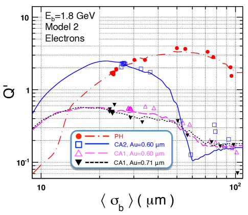
Figure 7: Comparison of the measured figures of merit $\mathcal{Q}_{Mj}^{\,\prime}({\sigma_{b}})$ (markers) for four optical elements (see text), with the corresponding predictions $\mathcal{Q}_{Pj}^{\,\prime}({\sigma_{b}})$ (curves) from model 2 for a ${E_{b}}=1.8$ ${\mathrm{GeV}}$ electron beam. Statistical uncertainties on the data points are smaller than the marker sizes.

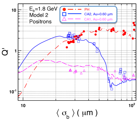
Figure 8: Comparison of the measured figures of merit $\mathcal{Q}_{Mj}^{\,\prime}({\sigma_{b}})$ (markers) for three optical elements (see text), with the corresponding predictions $\mathcal{Q}_{Pj}^{\,\prime}({\sigma_{b}})$ (curves) from model 2 for a ${E_{b}}=1.8$ ${\mathrm{GeV}}$ positron beam. Statistical uncertainties on the data points are smaller than the marker sizes.

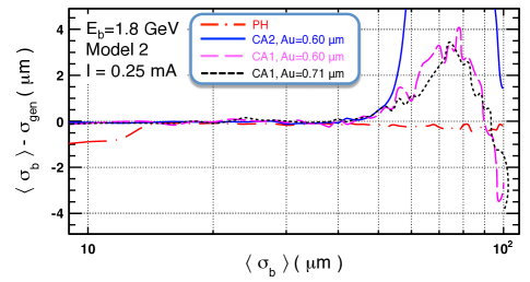
Figure 9: Bias in reconstructed vertical beam size for ${E_{b}}$=1.8 ${\mathrm{GeV}}$ and $I$=0.25 mA predicted by model 2 for various optical elements, as indicated.

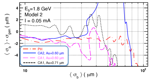
Figure 10: Bias in reconstructed vertical beam size for ${E_{b}}$=1.8 ${\mathrm{GeV}}$ and $I$=0.05 mA predicted by model 2 for various optical elements, as indicated.

The data confirm both models’ predictions that the CA2 pattern outperforms that of CA1 in our figure of merit at ${E_{b}}$=1.8 ${\mathrm{GeV}}$ and 2.1 ${\mathrm{GeV}}$ for beam sizes between 10 ${\mu\mathrm{m}}$ and 50 ${\mu\mathrm{m}}$. The CA1 design was inspired by the principles developed for a Uniformly Redundant Array (URA) [16, 17, 18], which has been used in x-ray astronomy and medical tomography. The primary reason that the URA-inspired CA1 performance does not approach that of CA2 or even the pinhole for ${\sigma_{b}}$$>$15 ${\mu\mathrm{m}}$ is that the URA concepts apply only when diffraction effects are minimal or non-existent (cf. Appendix). For the CESR-TA xBSM, however, diffraction makes major alterations to the image shape. The well known diffraction parameter $N=a^{2}/(\lambda L^{\,\prime})\sim 1$ would have to be at least an order of magnitude larger for diffraction effects to become unimportant. CA2 is effective precisely because it takes advantage of diffraction. The slit pattern details for CA2 were developed in an ad hoc, iterative method using model 1 as a performance predictor. Its figure of merit is very close to that of a simple 3-slit grid with 60 ${\mu\mathrm{m}}$ gaps and spacing (cf. Fig. 12 of Ref. [13]). The key to its effectiveness is that the slits are spaced closely enough for diffraction to sharpen the primary peaks in the image but spread apart enough that the primary peaks do not merge together.

Because model 2 involves a simulation that includes fitting images, it can also be used to predict the bias in fitted beam size, as shown in Figs. 9 and 10. At a current of 0.25 mA, the beam size bias at ${E_{b}}$=1.8 ${\mathrm{GeV}}$ for all four optical elements is negligible compared to 1 ${\mu\mathrm{m}}$ for ${\sigma_{b}}<50$ ${\mu\mathrm{m}}$, but can be large for the coded apertures above that beam size. This behavior occurs because the CA image begins to fill the entire detector with almost no discernable structure at such beam sizes. At lower current, however, the beam size bias becomes substantial and depends on the optic for its sign and size. Presumably this is caused by the assumption in the fitter of Gaussian statistics, whereas Poisson statistics begin to matter at lower current.

Finally, model 2, as calibrated to the data, may be used to determine the current dependence of the figure of merit. For a fixed beam energy and beam size, we expect it to be nearly constant at high current where statistics are dominantly Gaussian in nature, but to gradually decrease at lower currents where Poisson statistics begin to matter. Fig. 11 shows the predictions for three optical elements at ${E_{b}}$=1.8 ${\mathrm{GeV}}$ and ${\sigma_{b}}$=25 ${\mu\mathrm{m}}$ plotted with data of ${\sigma_{b}}$=22-25 ${\mu\mathrm{m}}$; above 4 mA, the beam size was significantly in excess of ${\sigma_{b}}$=25 ${\mu\mathrm{m}}$, so those data are omitted from the plot. Here the data and predictions are shown relative to the figure of merit at $I=1$ mA. The predictions are seen to level off at high current, as expected, at 4 mA for CA2 and 8 mA for the PH; the CA2 data, however, level off at about 2 mA, smaller than the prediction, perhaps due to unmodeled systematic effects increasing fluctuations in beam size.

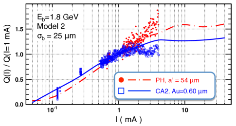
Figure 11: Current dependence of the figure of merit, $\mathcal{Q}({\sigma_{b}},I,H)$, at a fixed beam size ${\sigma_{b}}$=25 ${\mu\mathrm{m}}$ and horizontal illumination $H$, for ${E_{b}}$=1.8 ${\mathrm{GeV}}$ electrons. Solid circles (open squares) represent measurements using the PH (CA2) optical element, and the solid (dot-dashed) line the respective predictions of model 2.

4 Conclusions

We have reported on further data acquired with the CESR-TA x-ray vertical beam size monitor in order to more fully explore measured and predicted performance. A technique for standardizing measurements of beam size statistical resolving power to reference data has been described and implemented, allowing data taken at different currents and horizontal illuminations to be directly compared. The corrected data broadly confirm predictions of a new model. This model combines previously reported [13] methods to determine the point response function of any optical element with the detector image fitting procedure via construction of simulated images, including fluctuations due to x-ray photon statistics. The results verify that the tools developed are effective in design of coded apertures for specific current and beam size regimes. Pinhole optics optimized for gap size can function well for high current or large beam size situations, and avoid the physical fragility of coded apertures for high incident power. However, if low currents or very small beam sizes are expected, a beam size monitor can benefit from coded aperture optical elements. For beam sizes in the range of 10-50 ${\mu\mathrm{m}}$ in the ${E_{b}}$=2 ${\mathrm{GeV}}$ region, a particular five-slit coded aperture design in $\sim$0.7 ${\mu\mathrm{m}}$-thick gold plated on 2.5 ${\mu\mathrm{m}}$-thick silicon was measured to perform as predicted, better than a pinhole for ${\sigma_{b}}$$<$25 ${\mu\mathrm{m}}$ and better compared to our intial coded aperture with similar total light transmission for ${\sigma_{b}}$$<$50 ${\mu\mathrm{m}}$. Our results emphasize the importance of accounting for planned ranges of beam size and current as well as the incident x-ray spectrum and the effects of diffraction. The new model also predicts a non-negligible bias in measured beam size at very low beam current, an apparent consequence of x-ray photon statistics playing a significant role.

Appendix: URA Concepts & Limitations

Other x-ray imaging applications frequently need to reconstruct a complex source structure rather than measure the width of an assumed Gaussian distribution, as is done for the CESR-TA xBSM. They also usually have the advantage of operating in the non-diffractive regime, which simplifies the optics considerably. For both these reasons, such applications employ a figure of merit more general than described in Sect. 2 and hence arrive at different optimal aperture designs. Our optic CA1 was designed with an approach taken from observational astronomy, that of a Uniformly Redundant Array, or URA [16, 17, 18]. The purpose of this Appendix is, first, to show that in the non-diffractive limit, CA1 would indeed provide better resolving power than CA2, at least at small beam size; second, to describe the URA concept and limitations; and third, to demonstrate the failure of the URA formulation in realistic xBSM conditions.

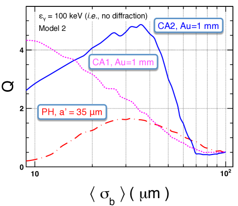
Figure 12: Predicted figure of merit for each of three optical elements at CESR-TA in the non-diffractive, thick-masking limit.

Before summarizing the URA concept, we briefly explore what the non-diffractive regime would look like with the CESR-TA geometry, using the tools described in this article. To do so we artificially restrict x-rays to be of energy $\epsilon=100$ ${\mathrm{keV}}$ instead of the $\approx 1-4$ ${\mathrm{keV}}$ energy range actually encountered [13]. We also assume thick masking, so that masked areas have zero transmission and slits have 100% transmission. In the absence of diffraction, apertures function as geometrically shadowing/anti-shadowing devices; through each slit a point source illuminates an area on the detector that is the slit size times the projection ratio, $1+M$. For a beam size of ${\sigma_{b}}\approx 15$ ${\mu\mathrm{m}}$ in this non-diffractive limit, the optimal size of a single slit (pinhole) for the CESR-TA geometry (Fig. 1) and detector is ${a^{\,\prime}}\approx 35$ ${\mu\mathrm{m}}$ (depending weakly upon beam current and the exact beam size in question), compared to ${a^{\,\prime}}=50$-60 ${\mu\mathrm{m}}$ for the actual x-rays at ${E_{b}}\approx 2$ ${\mathrm{GeV}}$. Figure 12 shows a comparison of the relative figures of merit of a 35 ${\mu\mathrm{m}}$ pinhole, CA1, and CA2 for 100 ${\mathrm{keV}}$ x-rays, as predicted by model 2. Below a beam size of about 14 ${\mu\mathrm{m}}$, the CA1 slit pattern obtains the best performance, validating the URA design in this non-diffractive limit. However, CA2 performs better for ${\sigma_{b}}$=14-65 ${\mu\mathrm{m}}$, in part due to its larger total light transmission (see Table 2). These are in stark contrast to results shown in Sect. 3, which, of course, include diffractive effects.

To facilitate source reconstruction, coded aperture imaging is commonly described [16, 17, 18] in terms of linear algebra: the aperture is segmented into equal size cells, and for each such cell a counterpart exists in both the source and image planes, with cell sizes scaled up from that of the aperture by factors $(1+M)/M$ and $1+M$, respectively. In this matrix formulation, the aperture can be described in terms of a matrix which maps each source pixel to a pattern on the image plane. For a 1-dimensional detector segmented into $N$ pixels, the source intensity distribution is represented as a $1\times N$ column vector $s$, the aperture is represented by an $N\times N$ matrix $A$, the image in the absence of detector noise is a $1\times N$ column vector $d=A\times s$, and the detector noise a $1\times N$ column vector $n$. The measured image, including noise, is $d^{\prime}$:

$$d^{\prime}\equiv d+n=A\times s+n\,.$$ (5)

Each row of $A$ represents the binned prf for a source located at a particular binned position. Each element $A_{ij}$ takes a value between 0 (completely opaque) and 1 (completely transmitting). To a good approximation, adjacent rows of $A$ are identical aside from a shift by one column, pulling in a zero to the trailing end of the row. Hence the entirety of $A$ can be trivially constructed from the binned prf. In this scheme, an approximation of the source, $s_{R}$, is reconstructed from the measured image by applying a matrix $G$:

$$s_{R}=G\times d^{\prime}=G\times A\times s+G\times n\,.$$ (6)

(It must be emphasized here that, while the rms noise values may be measured, the precise value of $n$ for any given image is not; only an average noise level can be removed from the measured image.) An obvious choice for $G$ is $A^{-1}$, but this is not always possible or desirable: $A$ can be singular, or nearly so. Some coded aperture patterns with nonsingular $A$ nonetheless have an $A^{-1}$ with very large elements, which in turn amplify the detector noise. Source reconstruction requires finding a matrix $G$ without individual elements that are large, and for which $G\times A$ is close to the identity matrix. The extent to which $G\times A$ differs from the identity matrix creates an artifact noise in $s_{R}$. The choice for $G$ should balance this artifact noise against amplified detector noise. The URA formulation applies to the situation of substantial and dominant detector noise, providing a prescription to design an aperture for which an effective $G$ may be constructed. One (narrow) definition of a URA is an aperture that has an autocorrelation function

$$\phi_{m}\equiv\sum_{j=1}^{N}A_{k,j}\;A_{k,j+m}$$ (7)

that is uniform (i.e., constant) for $k=(1+N)/2$ and $m=1,$ 2, 3, … , up to a significant fraction of $N$; crudely, a pattern for which the number of times transmitting segments are separated by any nonzero number of cells $m$ is the same for $m=1,2,3,...$.

Our optical element CA1 is a URA with $N=$31, and in the thick-masking limit the central ($k=16$) row of $A$ has the pattern

$$0110110111100010101110000100100,$$ (8)

where each digit corresponds to a 10 ${\mu\mathrm{m}}$-wide aperture segment. This URA has a nearly uniform redundancy, with $\phi_{m}=7,$ 7, 7, 6, 6, 7, 5, 5, 7 for $m=1-9$, respectively, which have an rms deviation of 14% of their mean.

The URA prescription for $G$ is:

$$G^{\prime}_{ij}=\dfrac{A_{ij}\;(2\rho-1)-\rho}{T\;(\,\rho-1\,)}\,,$$ (9)

where $\rho\equiv\left<A_{ij}\right>$ is the density of $A$ and $T=\sum_{j}A_{k,j}$ with $k=(1+N)/2$, is the total transparency. By construction, $G^{\prime}$ will generally not be $A^{-1}$. For the aperture of Eq. (8), the central row of $G^{\prime}\times A$ is plotted in Fig. 13 as the solid line: it shows a narrow, prominent spike (corresponding to each diagonal element) and smaller values elsewhere (corresponding to off-diagonal elements).

In contrast, if one approximates CA2 similarly, the thick-masking aperture is

$$1110111100001111111000011110111,$$ (10)

which has $\phi_{m}=16,$ 13, 10, 9, 10, 9, 8, 8, 8 for $m=1-9$, respectively. Thus, CA2 has far from uniform redundancy in the no-interference limit (with an rms variation of 27% of the mean redundancy), fails the URA requirements, and the URA prescription is not effective to use in source reconstruction.

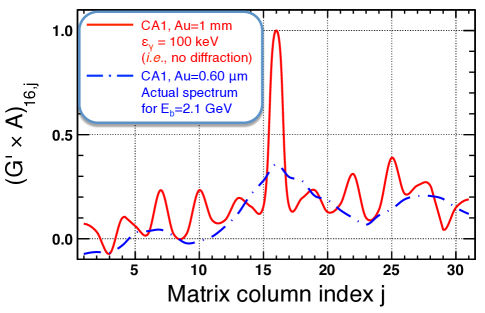
Figure 13: Central row of $G^{\prime}\times A$ (see text) in the URA formulation for the case of the coded aperture pattern CA1 in the no-diffraction, thick-masking limit (solid line) and actual conditions (dot-dashed line), which include the spectrum at ${E_{b}}$=2.1 ${\mathrm{GeV}}$, diffraction, and partial transmission through gold masking of thickness 0.6 ${\mu\mathrm{m}}$.

Diffraction unavoidably compromises the effectiveness of the URA formulation because the prf no longer tracks the aperture; i.e., the aperture is more than a shadowing/antishadowing device. An aperture which satisfies the URA criterion without diffraction is far from guaranteed to do so in the diffractive regime; i.e., redundancy will no longer be uniform. Using the CESR-TA geometry, the x-ray spectrum at ${E_{b}}$=2.1 GeV, and the CA1 aperture specifications, as well as phase-shifted, partial transmission through the gold masking, the redundancies are 8.8, 8.2, 7.5, 7.2, 6.6, 6.1, 5.7, 5.4, 5.3 for $m$=1-9, respectively. These redundancies have an rms variation of 19% of their mean. More importantly, the central row of the matrix $G^{\prime}\times A$, plotted in Fig. 13 as the dot-dashed line, has a much weaker and broader central spike relative to the diffraction-off result, so $G^{\prime}\times A$ will differ significantly from the identity matrix. Hence, for a realistic CA1, the viability of the URA prescription has disappeared.

Unlike most astronomical and medical imaging applications, the CESR-TA xBSM must operate in the diffractive regime. However, one can safely assume a single-peaked source of Gaussian shape, which allows image fitting with templated beam size to determine beam properties, as described in Ref. [13]. A beam-size-based figure of merit and an iterative, ad hoc procedure have been effective in optimizing a slit pattern (CA2) for low-power xBSM illuminations. The main body of this article documents measurements confirming that CA2 outperforms the URA-inspired CA1 by the expected factor, as a function of both beam size and current.

References

- [1] J. W. Flanagan et al., Conf. Proc. C 0806233 (2008) TUOCM02
- [2] J. Alexander et al., Proc. PAC09 TH5RFP026 (2009)
- [3] J. Alexander et al., Proc. PAC09 TH5RFP027 (2009)
- [4] J.W. Flanagan et al., Proc. PAC09, Vancouver, TH5RFP048 (2009)
- [5] J.W. Flanagan et al., Proc. PASJ10, Himeji, WEPS095 (2010)
- [6] J.W. Flanagan et al., Proc. IPAC10, Kyoto, MOPE007 (2010)
- [7] D. P. Peterson et al., Proc. IPAC10, Kyoto MOPE090 (2010)
- [8] J. W. Flanagan et al., Proc. DIPAC11 WEOB03 (2011)
- [9] N.T. Rider et al., Proc. PAC11 MOP304 (2011)
- [10] J. W. Flanagan, Conf. Proc. C 110904 (2011) 1959 (link)
- [11] N. T. Rider et al., Proc. IBIC12 WEDC01 (2012)
- [12] J. P. Alexander and D. P. Peterson, in Handbook of Accelerator Physics and Engineering, 2nd Ed., Edited by A. W. Chao, K. H. Mess, M. Tigner, F. Zimmerman, (World Scientific, Singapore, 2013) 721
- [13] J. P. Alexander et al., Nucl. Inst. and Methods in Physics Research, A 748C (2014) 96 (link)
- [14] R. H. Dicke, Astrophys. Journ. 153 (1968) L101 (link)
- [15] Applied NanoTools, Inc. #1200 –- 10045 111 Street, Edmonton, Alberta T5K 2M5, CANADA, www.appliednt.com
- [16] E. E. Fenimore and T. M. Cannon, Appl. Optics 17 (1978) 337 (link)
- [17] E. E. Fenimore, Appl. Optics 17 (1978) 3562 (link)
- [18] A. Busboom, H. Elders-Boll, and H. D. Schotten, Exp. Astron. 8 (1998) 97 (link)