CODING THEOREMS FOR HYBRID CHANNELS. II

Abstract

The present work continues investigation of the capacities of measurement (quantum-classical) channels in the most general setting, initiated in [10]. The proof of coding theorems is given for the classical capacity and entanglement-assisted classical capacity of the measurement channel with arbitrary output alphabet, without assuming that the channel is given by a bounded operator-valued density.

1 Introduction

The present work continues investigation of the capacities of measurement channels in the most general setting, initiated in [10]. The proof of coding theorems is given for the classical capacity (theorem 3) and entanglement-assisted classical capacity (theorem 4) of the measurement channel with arbitrary output alphabet under the minimal regularity assumptions. The statement of theorem 4 was proved previously in [10] under additional assumption that the channel is given by a bounded operator-valued density. In the present work we relax this restriction by using a generalization of the Radon-Nikodym theorem for probability operator-valued measures [6]. The result obtained is illustrated by an example of homodyne measurement in quantum optics.

We remark that the entanglement-assisted classical capacity was studied by a number of authors under the names purification capacity, measurement strength, forward classical communication cost. In the recent paper [2], where one can find further references, its alternative interpretation is developed. It is shown that a (finite-dimensional) measurement channel can be asymptotically simulated by transmission of a classical message of the size equal to the maximal entropy reduction, assisted with sufficient classical correlation between the input and the output. The result can be considered as a quantum reverse Shannon theorem in which entanglement and quantum channel are replaced, correspondingly, by classical correlation and classical channel.

2 Preliminaries

Let ${\mathcal{H}}$ be a separable Hilbert space. We use the following notations: $\mathfrak{B}(\mathcal{H})$  is the algebra of all bounded operators, $\mathfrak{T}(\mathcal{H})$  is the space of trace-class operators in $\mathcal{H}$, ${\mathfrak{S}}({\mathcal{H}})$  is its convex subset of density operators (i.e. positive operators with unit trace), called also quantum states.

We introduce the measure space $(\Omega,{\mathcal{F}},\mu),$ where $\Omega$  is a complete separable metric space, ${\mathcal{F}}$  is a $\sigma$-algebra of its subsets, $\mu$  is a $\sigma$-finite measure on ${\mathcal{F}}$. A hybrid (classical-quantum) system is described by von Neumann algebra ${\mathcal{L}}={\mathcal{L}}^{\infty}(\Omega,{\mathcal{F}},\mu;\mathfrak{B}(\mathcal{H}))$, consisting of weakly measurable, essentially bounded functions $X(\omega)$, $\omega\in\Omega$ with values in $\mathfrak{B}(\mathcal{H})$. Consider the preadjoint space ${\mathcal{L}}_{*}={\mathcal{L}}_{1}(\Omega,{\mathcal{F}},\mu;\mathfrak{T}(\mathcal{H})),$ the elements of which are measurable functions $S=\{S(\omega)\}$ with values in $\mathfrak{T}(\mathcal{H}),$ integrable with respect to the measure $\mu$. An element $S=\{S(\omega)\}\in{\mathcal{L}}_{*}$ such that

$$S(\omega)\geq 0\quad({\rm mod}\ \mu),\qquad\int_{\Omega}{\rm Tr}\,S(\omega)\,\mu(d\omega)=1,$$

is called state on the algebra ${\mathcal{L}}$. In notations of entropic characteristics of hybrid systems we will use the index “cq”, of classical and quantum systems — the indices “c” and “q” correspondingly.

Following [9], we introduce the notions of entropy and relative entropy of cq-states. Concerning the definitions and properties of quantum entropies see e. g. [8].

Definition 1. The entropy of a cq-state $S$ is defined by the relation

$$H_{\rm cq}(S)=\int_{\Omega}H_{q}(S(\omega))\,\mu(d\omega),$$

where $H_{q}(S)=-{\rm Tr}\,S\log S$  is the von Neumann entropy of positive operator $S\in\mathfrak{T}(\mathcal{H})$.

Note that

$$H_{\rm cq}(S)=H_{c}(p)+\int_{\Omega}p(\omega)H_{q}(\widehat{S}(\omega))\,\mu(d\omega),$$ (1)

where $p(\omega)={\rm Tr}\,S(\omega),$ $\widehat{S}(\omega)=(p(\omega))^{-1}S(\omega),$ $H_{c}(p)$  is the differential entropy of the probability distribution with the density $p(\omega)$ with respect to the measure $\mu$.

Definition 2. The relative entropy of cq-states $S_{1},S_{2}$ is defined by the relation

$$H_{\rm cq}(S_{1}\,\|\,S_{2})=\int_{\Omega}H_{q}(S_{1}(\omega)\,\|\,S_{2}(\omega))\,\mu(d\omega),$$

where

$$H_{q}(S_{1}(\omega)\,\|\,S_{2}(\omega))={\rm Tr}\,S_{1}(\omega)(\log S_{1}(\omega)-\log S_{2}(\omega))$$

is the quantum relative entropy.

To describe measurement channels we will need the following definition.

Definition 3. Probability operator-valued measure $($POVM$)$ on $\Omega$ is a family $M=\{M(A),\ A\in{\mathcal{F}}\}$ of bounded Hermitian operators in $\mathcal{H},$ satisfying the conditions:

$1)$ $M(A)\geq 0,$ $A\in{\mathcal{F}};$

$2)$ $M(\Omega)=I,$ where $I$ is the unit operator in $\mathcal{H}$;

$3)$ for arbitrary countable decomposition $A=\bigcup A_{i}$ $(A_{i}\cap A_{j}=\varnothing,\ i\neq j)$, the relation $M(A)=\sum_{i}M(A_{i})$ holds in the sense of weak convergence of operators.

POVM defines a quantum observable with values in $\Omega$. The probability distribution of observable $M$ in the state $S$ is given by the formula

$$P_{S}(A)={\rm Tr}\,SM(A),\qquad A\in{\mathcal{F}}.$$ (2)

For brevity, we sometimes write $P_{S}(d\omega)={\rm Tr}\,SM(d\omega)$.

If POVM $M(d\omega)$ is defined by the density $P(\omega)$ with respect to scalar $\sigma$-finite measure $\mu,$ where $P(\omega)$  is a uniformly bounded (with respect to the oprator norm) weakly measurable operator-valued function, then its probability distribution has the density $p_{S}(\omega)={\rm Tr}\,SP(\omega)$ with respect to the measure $\mu$. This case is studied in [10].

In the general case the following lemma holds (a generalization of the Radon-Nikodym theorem for POVM [6]).

Lemma 1. For an arbitrary POVM on a separable metric space  $\Omega$ there exist a dense subspace ${\mathcal{D}}\in\mathcal{H},$ a $\sigma$-finite measure $\mu$ on $\Omega,$ a countable set of Borel functions $\omega\rightarrow a_{k}(\omega)$ where for almost all $\omega$ the $a_{k}(\omega)$ are linear functionals on ${\mathcal{D}},$ satsfying the conditions

$$\int_{\Omega}\sum_{k}|\langle a_{k}(\omega)|\psi\rangle|^{2}\,\mu(d\omega)=\|\psi\|^{2},\qquad\psi\in{\mathcal{D}},$$ (3)

$$\langle\psi|M(A)\psi\rangle=\int_{A}\sum_{k}|\langle a_{k}(\omega)|\psi\rangle|^{2}\,\mu(d\omega),\qquad\psi\in{\mathcal{D}}.$$ (4)

In [6] it is shown that for ${\mathcal{D}}$ one can take ${\rm lin}\,\{\varphi_{i}\}$ — the linear span of a fixed orthonormal basis $\{\varphi_{i}\}$ .

Lemma 2. For arbitrary observable $M(d\omega)$ with values in $\Omega$ and a density operator $S\in\mathfrak{S}(\mathcal{H})$, the probability distribution $P_{S}(d\omega)={\rm Tr}\,SM(d\omega)$ has density $p_{S}(\omega)$ with respect to measure $\mu$.

Proof. Consider the spectral decomposition of the state $S$:

$$S=\sum_{i=1}^{\infty}\lambda_{i}|\varphi_{i}\rangle\langle\varphi_{i}|.$$ (5)

Apply lemma 2, with ${\mathcal{D}}={\rm lin}\{\varphi_{i}\}$. For all $A\in{\mathcal{F}}$ the equality holds

$$P_{S}(A)\equiv{\rm Tr}\,SM(A)=\int_{A}p_{S}(\omega)\,\mu(d\omega),$$ (6)

where

$$p_{S}(\omega)=\sum_{i=1}^{\infty}\lambda_{i}\sum_{k}|\langle a_{k}(\omega)|\varphi_{i}\rangle|^{2}$$

is a nonnegative integrable function is a nonnegative integrable function by the condition (3) and the spectral decomposition (5). The lemma is proved.

Let us fix an orthonormal system $\{e_{k}\}$ in $\mathcal{H}$. According to the same conditions (3) and (5), the relation

$$\widehat{S}(\omega)=(p_{S}(\omega))^{-1}\sum_{i=1}^{\infty}\lambda_{i}\sum_{j,k}|e_{k}\rangle\langle a_{k}(\omega)|\varphi_{i}\rangle\overline{\langle a_{j}(\omega)|\varphi_{i}\rangle}\langle e_{j}|$$ (7)

for $P_{S}$-almost all $\omega$ defines a density operator in $\mathcal{H}$, which we will call posterior state. The meaning of this term is that under certain conditions the operator $\widehat{S}(\omega)$ describes state of the quantum system after measurement of observable $M$, which resulted with the outcome $\omega$ [8].

Following [7], define the entropy reduction by the relation

$${\rm ER}\,(S,M)=H_{q}(S)-\int_{\Omega}p(\omega)H_{q}(\widehat{S}(\omega))\,\mu(d\omega),$$ (8)

which is consistent provided $H_{q}(S)<\infty$. We mention the following approximation properties. Consider a sequence of states $S_{n}=\sum_{i=1}^{n}\widetilde{\lambda_{i}}|\varphi_{i}\rangle\langle\varphi_{i}|,$ where $\widetilde{\lambda_{i}}=(\sum_{k=1}^{n}\lambda_{k})^{-1}\lambda_{i}.$ By lemma 4 of the paper [11], the above sequence $S_{n}$ satisfies the condition

$$\lim_{n\rightarrow\infty}H_{q}(S_{n})=H_{q}(S)<\infty.$$ (9)

According to the theorem 2 from [7], this implies

$$\lim_{n\rightarrow\infty}{\rm ER}\,(S_{n},{M})={\rm ER}\,(S,{M})<\infty.$$ (10)

3 The classical capacity of a measurement channel

Definition 4.  Let $M$ be a POVM, $P_{S}$ — its probability distribution in the state $S$, which is given by the formula (2). Measurement channel $\mathcal{M}$ is an affine map $S\rightarrow P_{S}(d\omega)$ of the convex set of quantum states ${\mathfrak{S}}(\mathcal{H})$ into the set of probability distributions on $\Omega$.

To apply the method of block coding, we need to define the $n$-th degree $\mathcal{M}^{\otimes n}$ of the channel $\mathcal{M}$. Let $\mathcal{H}^{\otimes n}$ be the $n$-th tensor degree of the Hilbert space $\mathcal{H}$ and let $(\Omega^{\times n},{\mathcal{F}}^{\times n})$ be the product of $n$ copies of the measurable space $(\Omega,{\mathcal{F}})$. The cnannel $\mathcal{M}^{\otimes n}$ is defined by the observable $M^{\otimes n}$ with values in $\Omega^{\times n}$ such that

$$M^{\otimes n}(A_{1}\times\cdots\times A_{n})=M(A_{1})\otimes\cdots\otimes M(A_{n}).$$

By using an analog of the extension theorem for POVM, one can show that this relation defines uniquely all the values $M^{\otimes n}(A^{(n)})$, $A^{(n)}\in{\mathcal{F}}^{\times n}.$

In the case of infinite-dimensional $\mathcal{H}$ one usually introduces a constraint onto the input states of the channel (otherwise the capacities are infinite as a rule). Let $F$ be a positive selfadjoint (in general unbounded) operator in the space $\mathcal{H}$, with the spectral decomposition $F=\int_{0}^{\infty}x\,dE(x),$ where $E(x)$ is the spectral function. We introduce the subset of states

$${\mathcal{A}}_{E}=\{S\in\mathfrak{S}(\mathcal{H}):{\rm Tr}\,SF\leq E\},$$ (11)

where $E$ is a positive constant, and the trace in (11) is understood as the integral $\int_{0}^{\infty}x\,d({\rm Tr}\,SE(x))$ (for more detail see [3]). Notice that if the operator $F$ satisfies the condition

$${\rm Tr}\,\exp(-\beta F)<\infty\quad\mbox{ }\ \beta>0,$$ (12)

then $H_{q}(S)<\infty$ for all $S$ such that ${\rm Tr}\,SF\leq E$ (see [3]). The corresponding constraint for the channel $\mathcal{M}^{\otimes n}$ is determined by the operator

$$F^{(n)}=F\otimes I\otimes\cdots\otimes I+\cdots+I\otimes I\otimes\cdots\otimes F.$$

Denote

$${\mathcal{A}}^{(n)}_{E}=\{S^{(n)}\in\mathfrak{S}(\mathcal{H}^{\otimes n}):{\rm Tr}\,S^{(n)}F^{(n)}\leq nE\}.$$ (13)

Definition 5. The code of length $n$ and size $N$ is a pair $(\Sigma^{(n)},{\mathcal{V}}^{(n)})$, where:

1) $\Sigma^{(n)}=\{S_{i}^{(n)},\ i=1,\ldots,N\}$ is a family of states from ${\mathcal{A}}_{E}^{(n)}$;

2) ${\mathcal{V}}^{(n)}=\{V_{j},\ j=0,1,\ldots,N\}$ is a decomposition of the space $\Omega^{\times n}$.

Definition 6. The average error probability of the code $(\Sigma^{(n)},{\mathcal{V}}^{(n)})$ is the quantity

$$\overline{u}(\Sigma^{(n)},{\mathcal{V}}^{(n)})=\frac{1}{N}\sum_{j=1}^{N}\big{(}1-{\rm Tr}\,S_{j}^{(n)}M^{\otimes n}(V_{j})\big{)}.$$ (14)

We denote by $u(n,N)$ the greatest lower bound of the quantity $\overline{u}(\Sigma^{(n)},{\mathcal{V}}^{(n)})$ with respect to all codes of length $n$ and size $N$.

Definition 7. We call the classical capacity $C({\mathcal{M}},{\mathcal{A}}_{E})$ of the measurement channel ${\mathcal{M}}$ with the constraint (13) the supremum of all achievable rates i.e. the values $R>0$, satisfying the condition

$$\lim_{n\rightarrow\infty}u(n,2^{nR})=0.$$ (15)

We call by ensemble of states a finite probability distribution $\pi=\{\pi_{x};S_{x}\}$ on the set of states ${\mathfrak{S}}({\mathcal{H}})$, ascribing probabilities $\pi_{x}$ to certain states $S_{x}$. The average state of ensemble is defined as: $\overline{S}_{\pi}=\sum_{x}\pi_{x}S_{x}$. Let us denote ${\mathcal{P}}_{E}$ the set of ensembles $\pi$ such that $\overline{S}_{\pi}\in{\mathcal{A}}_{E}$; similarly, we denote ${\mathcal{P}}_{E}^{(n)}$ the set of ensembles $\pi^{(n)}$ in $\mathfrak{S}(\mathcal{H}^{\otimes n})$, the average state of which satisfying the condition (13).

For given measurement channel ${\mathcal{M}}$ and ensemble $\pi$ define the quantity

$$I(\pi,{\mathcal{M}})=\sum_{x}\pi_{x}\int_{\Omega}p(\omega|x)\log\frac{p(\omega|x)}{\overline{p}(\omega)}\,\mu(d\omega).$$ (16)

Here $\overline{p}(\omega)$ and $p(\omega|x)$ are the probability densities of the distributions $\overline{P}(d\omega)={\rm Tr}\,\overline{S}_{\pi}M(d\omega)$ and $P_{x}(d\omega)={\rm Tr}\,S_{x}M(d\omega)$ correspondingly. The quantity $I(\pi,{\mathcal{M}})$ is the Shannon mutual information between the discrete random variable $X$, having the probability distribution $\{\pi_{x}\}$ and the random variable $\omega$ with conditional probability density $p(\omega\,|\,x)$, defined via lemma 2. Notice that there is a representation of the quantity $I(\pi,{\mathcal{M}})$ as a supremum over decompositions ${\mathcal{V}}=\{V_{i}\}$ of the output space $\Omega$ (cf. [5, formula (1.2.3)]):

$$I(\pi,{\mathcal{M}})=\sup_{{\mathcal{V}}}\bigg{(}\sum_{i}\sum_{x}\pi_{x}P_{x}(V_{i})\log\frac{P_{x}(V_{i})}{\overline{P}(V_{i})}\bigg{)}.$$ (17)

The quantity under supremum is equal to $I(\pi,{\mathcal{M}}_{\mathcal{V}})$, where ${\mathcal{M}}_{\mathcal{V}}$ is the measurement channel, corresponding to the discrete observable $\{M(V_{i})\}$.

Theorem 1.  The classical capacity of the measurement channel $\mathcal{M}$ with the constraint (13) is given by the relation

$$C(\mathcal{M},{\mathcal{A}}_{E})=\sup_{\pi\in{\mathcal{P}}_{E}}I(\pi,{\mathcal{M}}).$$ (18)

Proof. Denote

$$C_{n}=\sup_{\pi^{(n)}\in{\mathcal{P}}^{(n)}_{E}}I(\pi^{(n)},{\mathcal{M}}^{\otimes n}).$$

We need to show that

$$C(\mathcal{M},{\mathcal{A}}_{E})=C_{1}.$$

Let us first establish the additivity property $C_{n}=nC_{1}$.

For a fixed decomposition ${\mathcal{V}}=\{V_{i}\}$, the measurement channel ${\mathcal{M}}_{\mathcal{V}}$ is embedded into quantum entanglement-breaking channel (see e.g. [4]), therefore according to [3] its capacity is given by the expression

$$C({\mathcal{M}}_{\mathcal{V}},{\mathcal{A}}_{E})=\sup_{\pi\in{\mathcal{P}}_{E}}I(\pi,{\mathcal{M}}_{\mathcal{V}}),$$ (19)

and has the additivity property (see [6])

$$C({\mathcal{M}}^{\otimes n}_{\mathcal{V}},{\mathcal{A}}^{(n)}_{E})=nC({\mathcal{M}}_{\mathcal{V}},{\mathcal{A}}_{E}).$$

Notice that similarly to (19), the left-hand side is equal to $\sup_{\pi^{(n)}\in{\mathcal{P}}^{(n)}_{E}}I(\pi^{(n)},{\mathcal{M}}^{\otimes n}_{\mathcal{V}})$, so that

$$\sup_{\pi^{(n)}\in{\mathcal{P}}^{(n)}_{E}}I(\pi^{(n)},{\mathcal{M}}^{\otimes n}_{\mathcal{V}})=n\sup_{\pi\in{\mathcal{P}}_{E}}I(\pi,{\mathcal{M}}_{\mathcal{V}}).$$ (20)

By using a result of R. L. Dobrushin (theorem 2.2 in [5]), we have

$$I(\pi^{(n)},{\mathcal{M}}^{\otimes n})=\sup_{{\mathcal{V}}}I(\pi^{(n)},{\mathcal{M}}^{\otimes n}_{\mathcal{V}}),$$

because the supremum in the right-hand side is equal to the supremum of the information with respect to decompositions of the space $\Omega^{\times n}$ of special form, consisting of products $V_{1}\times\cdots\times V_{n}$ of the sets from the decomposition ${\mathcal{V}}$. The class of all such products has the ordering property that is required for validity of theorem 2.2 in [5]. Hence

$$C_{n} = \sup_{\pi^{(n)}\in{\mathcal{P}}^{(n)}_{E}}\sup_{{\mathcal{V}}}I(\pi^{(n)},{\mathcal{M}}^{\otimes n}_{\mathcal{V}})=\sup_{{\mathcal{V}}}\sup_{\pi^{(n)}\in{\mathcal{P}}^{(n)}_{E}}I(\pi^{(n)},{\mathcal{M}}^{\otimes n}_{\mathcal{V}})$$

$$= n\sup_{{\mathcal{V}}}\sup_{\pi\in{\mathcal{P}}_{E}}I(\pi,{\mathcal{M}}_{\mathcal{V}})=n\sup_{\pi\in{\mathcal{P}}_{E}}\sup_{{\mathcal{V}}}I(\pi,{\mathcal{M}}_{\mathcal{V}})$$

$$= n\sup_{\pi\in{\mathcal{P}}_{E}}I(\pi,{\mathcal{M}})=nC_{1},$$

where we used (20) in the third equality.

Now let us prove the inequality $C({\mathcal{M}},{\mathcal{A}}_{E})\leq C_{1}.$ Without loss of generality we can suppose that $C_{1}<\infty.$ Let $R>C_{1}.$ By applying Fano’s inequality, we obtain similarly to the relation (10.19) in [8]

$$u(n,2^{nR})\geq 1-\frac{C_{n}}{nR}-\frac{1}{nR}=1-\frac{C_{1}}{R}-\frac{1}{nR},$$

where in the second equality we used the additivity $C_{n}=nC_{1}$. Therefore $\liminf_{n\rightarrow\infty}u(n,2^{nR})>0$, and hence $C({\mathcal{M}},{\mathcal{A}}_{E})\leq C_{1}.$

For the proof of the converse inequality we note that

$$C({\mathcal{M}},{\mathcal{A}}_{E})\geq C({\mathcal{M}}_{{\mathcal{V}}},{\mathcal{A}}_{E})=\sup_{\pi\in{\mathcal{P}}_{E}}I(\pi,{\mathcal{M}}_{\mathcal{V}})$$

for arbitrary decomposition ${\mathcal{V}}$. By taking supremum over the decompositions ${\mathcal{V}}$, we obtain $C({\mathcal{M}},{\mathcal{A}}_{E})\geq\sup_{\pi\in{\mathcal{P}}_{E}}I(\pi,{\mathcal{M}})=C_{1}$. The theorem 1 is proved.

4 Entanglement-assisted capacity of a measurement channel

Consider the following protocol of classical information transmission through the measurement channel $\mathcal{M}$. Transmitter $A$ and receiver $B$ are in the pure entangled state $S_{AB}=|\psi\rangle\langle\psi|$, where $|\psi\rangle=\sum_{j}c_{j}|e_{j}\rangle\otimes|\widetilde{e_{j}}\rangle,$ satisfying the condition $H_{q}(S_{A})=H_{q}(S_{B})<\infty.$

Let ${\mathcal{X}}$ be a finite alphabet, and the classical signal $x\in{\mathcal{X}}$ appears with probability $\pi_{x}$. The party $A$ performs encoding $x\rightarrow{\mathcal{E}}_{x}$ and sends its part of the resulting common state via the channel $\mathcal{M}$. Thus the party $B$ has at its disposal the hybrid system $\Omega B$, where $\Omega$ is the classical system at the output of the measurement channel. After the measurement of observable $M(d\omega)$, the state in the hybrid system is described in the following way:

$$\sigma_{x}(d\omega)=\sum_{j,k}c_{j}\overline{c}_{k}[{\rm Tr}\,{\mathcal{E}}_{x}(|e_{j}\rangle\langle e_{k}|)M(d\omega)]|\widetilde{e}_{j}\rangle\langle\widetilde{e}_{k}|.$$

Then the party $B$ may perform measurement of an observable in the system $\Omega B$, extracting in this way information about the signal $x$.

With the block coding, the encoded states transmitted through the channel $\mathcal{M}^{\otimes n}\otimes{\rm Id}\,_{B}^{\otimes n}$, have the form

$$S_{\alpha}^{(n)}=({\mathcal{E}}_{\alpha}^{(n)}\otimes{\rm Id}\,_{B}^{\otimes n})[S_{AB}^{(n)}],$$ (21)

where $S_{AB}^{(n)}$ is pure entangled state for $n$ copies of the system $AB$, satisfying the condition $H(S_{B}^{(n)})<\infty,$ $\alpha$ is the classical message (e.g. a word in an alphabet ${\mathcal{X}}$), $\alpha\rightarrow{\mathcal{E}}_{\alpha}^{(n)}$ are the encodings for $n$ copies of the system $A$. The input states of the channel $\mathcal{M}^{\otimes n}$ are subject to the constraint (13), which is equivalent to similar constraint for the channel $\mathcal{M}^{\otimes n}\otimes{\rm Id}\,_{B}^{\otimes n}$ with the operators $F^{(n)}\otimes I_{B}^{\otimes n}.$

For the channel $\mathcal{M}$ with the input constraint (11) we consider the quantity

$$C_{\rm ea}^{(n)}(\mathcal{M}^{\otimes n},{\mathcal{A}}_{E}^{(n)})=\sup_{(\pi^{(n)}_{\alpha},S^{(n)}_{\alpha})}\chi_{\rm cq}\left(\{\pi_{\alpha}^{(n)}\};\{(\mathcal{M}^{\otimes n}\otimes{\rm Id}\,_{B}^{\otimes n})S^{(n)}_{\alpha}\}\right),$$ (22)

where

$$\chi_{\rm cq}\left(\{\pi_{x}\};\{S_{x}\}\right)=H_{\rm cq}\bigg{(}\sum_{x}\pi_{x}S_{x}\bigg{)}-\sum_{x}\pi_{x}H_{\rm cq}(S_{x}),\qquad S_{x}\in{\mathcal{L}}_{*},$$

and the supremum is taken over all state ensembles of the form (21), satisfying the condition

$$\sum_{\alpha}\pi^{(n)}_{\alpha}{\rm Tr}\,S^{(n)}_{\alpha}(F^{(n)}\otimes I_{B}^{\otimes n})\leq nE.$$

The classical entanglement-assisted capacity for the quantum-classical channel $\mathcal{M}$ with the constraint (11) is defined by the relation

$$C_{\rm ea}(\mathcal{M},{\mathcal{A}}_{E})=\lim_{n\rightarrow\infty}\frac{1}{n}\,C_{\rm ea}^{(n)}(\mathcal{M}^{\otimes n},{\mathcal{A}}_{E}^{(n)}).$$

Theorem 2.  Let $\mathcal{M}$ be an arbitrary measurement channel with the input constraint (13). Assume, that the operator $F$ satisfies the condition (12), and the channel $\mathcal{M}$ satisfies the condition

$$\sup_{S_{A}:{\rm Tr}\,S_{A}F\leq E}H_{c}(p_{S_{A}})<\infty,$$ (23)

where $H_{c}(p_{S_{A}})$ is the classical differential entropy of the probability density of the output distribution of the channel $\mathcal{M}$. Then the entanglement-assisted capacity is given by the expression

$$C_{\rm ea}(\mathcal{M},{\mathcal{A}}_{E})=\sup_{S_{A}:{\rm Tr}\,S_{A}F\leq E}{\rm ER}\,(S_{A},M).$$ (24)

Proof. In the proof we use the corresponding result for measurement channels defined by a bounded operator density, obtained in [10].

Let $S_{AB}$ be the initial entangled state of the system $AB$. After applying encoding ${\mathcal{E}}_{A}^{x}$ in the system $A$ the state of the composite system is described by the operator

$$S_{AB}^{x}=({\mathcal{E}}_{A}^{x}\otimes{\rm Id}\,_{B})S_{AB}$$

with the partial states $S_{A}^{x}={\mathcal{E}}_{A}^{x}(S_{A})$ and $S_{B}^{x}=S_{B}$.

To establish the inequality $\leq$ in the formula (24), it is sufficient to prove (see [10] for detail) that

$$H_{\rm cq}\bigg{(}\sum_{x}\pi_{x}(\mathcal{M}\otimes{\rm Id}\,_{B})S^{x}_{AB}\bigg{)}-\sum_{x}\pi_{x}H_{\rm cq}\left(\mathcal{M}\otimes{\rm Id}\,_{B}(S_{AB}^{x})\right)\leq{\rm ER}\,(\overline{S}_{A},M).$$ (25)

Here $\overline{S}_{A}=\sum_{x}\pi_{x}S_{A}^{x}$, and the constraint (13) implies the condition

$${\rm Tr}\,\overline{S}_{A}F\leq E.$$ (26)

A result of [10] implies that the relation (25) holds for finite-rank states $\overline{S}_{A}$ satisfying the constraint (26). For the proof in the general case we apply approximation by finite-rank states.

Assume first that ${\rm Tr}\,\overline{S}_{A}F\leq E^{\prime}<E$ for a positive $E^{\prime}.$ Let $\overline{S}_{A}$ have the spectral decomposition $\overline{S}_{A}=\sum_{i}\lambda_{i}|\varphi_{i}\rangle\langle\varphi_{i}|$. Consider the increasing sequence of projections $P_{n}=\sum_{i=1}^{n}|\varphi_{i}\rangle\langle\varphi_{i}|$ converging to the unit operator $I_{A}$, and the sequence of states

$$S_{AB}^{x}(n)=P_{n}\otimes I_{B}S_{AB}^{x}P_{n}\otimes I_{B}+|\phi\rangle\langle\phi|\otimes(S_{B}-S_{B}^{x}(n)),$$

where $S_{B}^{x}(n)={\rm Tr}\,_{A}(P_{n}\otimes I_{B}S_{AB}^{x}P_{n}\otimes I_{B}),$ $|\phi\rangle$ is a fixed unit vector from ${\rm lin}\{\varphi_{i}\}$, belonging to the domain of $\sqrt{F}$. The partial states of $S_{AB}^{x}(n)$ are

$${\rm Tr}\,_{B}S_{AB}^{x}(n)=S_{A}^{x}(n)=P_{n}S_{A}^{x}P_{n}+(1-{\rm Tr}\,P_{n}S_{A}^{x})|\phi\rangle\langle\phi|,\quad{\rm Tr}\,_{A}S_{AB}^{x}(n)=S_{B}.$$

Then the average state in the system $A$ is equal to

$$\overline{S}_{A}(n)=\sum_{x}\pi_{x}S_{A}^{x}(n)=P_{n}\overline{S}_{A}P_{n}+(1-{\rm Tr}\,P_{n}\overline{S}_{A})|\phi\rangle\langle\phi|.$$

We have $\overline{S}_{A}(n)=\sum_{i=1}^{n}{\lambda_{i}}|\varphi_{i}\rangle\langle\varphi_{i}|+(1-{\rm Tr}\,P_{n}\overline{S}_{A})|\phi\rangle\langle\phi|,$ then $\|\overline{S}_{A}(n)-\overline{S}_{A}\|_{1}\rightarrow 0$ for $n\rightarrow\infty$ and

$${\rm Tr}\,\overline{S}_{A}(n)F=\sum_{i=1}^{n}{\lambda}_{i}\|\sqrt{F}\varphi_{i}\|^{2}+(1-{\rm Tr}\,P_{n}\overline{S}_{A})\langle\phi|F\phi\rangle\leq E^{\prime}+\varepsilon_{n},$$

$\varepsilon_{n}\rightarrow 0$ $n\rightarrow\infty.$ Thus, starting from some value of $n$, the density operator $\overline{S}_{A}(n)$ satisfies the input constraint (26).

Using the condition (23), similarly to the proof of the coding theorem for measurement of observable in [10] we obtain the inequality (25) for the ensemble $\{\pi_{x},S^{x}_{AB}(n)\},$ which can be written in the following form based on the relative entropy:

$$\sum_{x}{\pi}_{x}H_{\rm cq}\bigg{(}(\mathcal{M}\otimes{\rm Id}\,_{B})(S^{x}_{AB}(n))\,\bigg{\|}\,\sum_{x}{\pi}_{x}(\mathcal{M}\otimes{\rm Id}\,_{B})S^{x}_{AB}(n)\bigg{)}\leq{\rm ER}\,({\rm Tr}\,\overline{S}_{A}(n),M).$$ (27)

Take the limit $n\rightarrow\infty$ in (27). By noting that $\lim_{n\rightarrow\infty}H_{q}(\overline{S}_{A}(n))=H_{q}(\overline{S}_{A})$, using theorem 2 from [7] (i.e. the equality (10)) in the left-had side and the lower semicontinuity of the relative entropy in the right-hand side, we obtain (25) for the ensemble $\{\pi_{x},S^{x}_{AB}\}$.

Now consider the case ${\rm Tr}\,\overline{S}_{A}F=E$. Take a unit vector $|e\rangle\in{\rm lin}\{\phi_{i}\},$ satisfying the condition $\langle e|Fe\rangle<E,$ and construct the approximation $S^{x}_{AB}(\varepsilon)=(1-\varepsilon)S^{x}_{AB}+\varepsilon|e\rangle\langle e|\otimes S_{B},~{}0<\varepsilon<1.$ Then the average state of the system $A$ is $\overline{S}_{A}({\varepsilon})=(1-\varepsilon)\overline{S}_{A}+\varepsilon|e\rangle\langle e|$, and the following condition holds

$${\rm Tr}\,\overline{S}_{A}({\varepsilon})F<E.$$

Let us repeat previous argument approximating $S^{x}_{AB}(\varepsilon)$ by the states of the form

$$(1-\varepsilon)P_{n}\otimes I_{B}S^{x}_{AB}P_{n}\otimes I_{B}+|e\rangle\langle e|(S_{B}-(1-\varepsilon){\rm Tr}\,_{A}P_{n}\otimes I_{B}S^{x}_{AB})$$

with the partial states $(1-\varepsilon)S_{A}^{x}+(1-(1-\varepsilon){\rm Tr}\,P_{n}S_{A}^{x})|e\rangle\langle e|$ and $S_{B}$ in the systems $A$ and $B$ correspondingly. We obtain that the inequality (25) holds for $S^{x}_{AB}(\varepsilon)$, $\overline{S}_{A}({\varepsilon})$. Since $\lim_{\varepsilon\rightarrow 0}H_{q}(\overline{S}_{A}({\varepsilon}))=H_{q}(\overline{S}_{A}),$ then, tending $\varepsilon$ to zero we obtain (25) for ensembles satisfying the condition ${\rm Tr}\,\overline{S}_{A}F=E$. The rest of the proof is similar to the case of observable with a bounded density [10].

To prove the inequality $\geq$ in (24) we consider an arbitrary state $S\in\mathfrak{S}(\mathcal{H})$, $S=\sum_{i=1}^{\infty}\lambda_{i}|\varphi_{i}\rangle\langle\varphi_{i}|,$ satisfying the input constraint. Apply lemma 1, setting ${\mathcal{D}}={\rm lin}\,\{\varphi_{i}\}$ and defining posterior states $\widehat{S}(\omega)$ by the relation (7). Then the argument is similar to trhe proof of proposition 4 from [3], and also theorem 3 from [10]. Theorem 2 is proved.

Of special interest is the case of pure POVM for which there exists a representation (4) of the form

$$\langle\psi|M(A)\psi\rangle=\int_{A}|\langle a(\omega)|\psi\rangle|^{2}\,\mu(d\omega),\qquad\psi\in{\mathcal{D}}.$$ (28)

In this case the posterior state (7) is a pure state, not depending on $x$:

$$\widehat{S}(\omega)=|e\rangle\langle e|,$$ (29)

where $e\in{\mathcal{H}}$ is a unit vector. Thus, $H_{q}(\widehat{S}(\omega))=0$ and the entropy reduction is equal to

$${\rm ER}\,(S,M)=H_{q}(S).$$ (30)

The relation (24) takes the form

$$C_{\rm ea}(\mathcal{M},{\mathcal{A}}_{E})=\sup_{S_{A}:{\rm Tr}\,S_{A}F\leq E}H_{q}(S).$$ (31)

It is well known that this supremum is attained on the Gibbs state

$$S_{\beta}=c(\beta)^{-1}\exp(-\beta F),\qquad c(\beta)={\rm Tr}\,\exp(-\beta F),$$ (32)

where $\beta$ is found from the condition ${\rm Tr}\,S_{\beta}F=E$, and it is equal to $\beta E+c(\beta)$. Thus theorem 4 implies the following statement.

Corollary 1. For arbitrary measurement channel, corresponding to pure POVM,

$$C_{\rm ea}(\mathcal{M},{\mathcal{A}}_{E})=\beta E+c(\beta),$$

where $\beta$ is found from the condition ${\rm Tr}\,S_{\beta}F=E$.

Let us illustrate this result by two examples. Let ${\mathcal{H}}=L^{2}(\mathbf{R})$, $Q$ be the operator of multiplication by $x$, $P=-id/dx$ with the common essential domain ${\mathcal{D}}={\mathcal{S}}(\mathbf{R})$ (the space of infinitely differentiable functions rapidly decreasing with all derivatives, see e.g. [8]). The spectral measure $M$ of the selfadjoint operator $Q$ can be represented in the form  (28):

$$\langle\psi|M(A)\psi\rangle=\int_{A}|\langle x|\psi\rangle|^{2}\,dx,\qquad\psi\in{\mathcal{S}}({\mathbf{R}}),$$

where $\langle x|\psi\rangle=\psi(x)$, $\psi\in{\mathcal{S}}(\mathbf{R})$, are the Dirac’s $\delta$-functionals. Thus the POVM $M$ does not have bounded operator density, the result of the paper [10] is not applicable and one should apply the approach of the present paper. Arbitrary density operator $S$ in $L^{2}(\mathbf{R})$ is defined by the kernel which is conveniently written in the symbolic form $\langle x|S|y\rangle$ (for continuous kernels this notation can be understood literally). Consider the channel corresponding to the measurement of observable $Q$, which maps a density operator $S$ into the probability density $\langle x|S|x\rangle$ with respect to the Lebesgue measure on the real line. In quantum optics such a channels describes statistics of homodyne measurement of one mode $Q,P$ of electromagnetic field [12]. As a constraint operator one usually takes the oscillator energy $F=(P^{2}+Q^{2})/2$. Notice that the condition (23) is fulfilled, as the inequality ${\rm Tr}\,SF\leq E$ implies

$$\int x^{2}p_{S}(x)\,dx={\rm Tr}\,SQ^{2}\leq 2{\rm Tr}\,SF\leq 2E,$$

and the maximal differential entropy (equal to $(1/2)\log(2\pi e(2E))$) under this constraint is attained on the Gaussian probability density. Substituting this value of supremum, equal to the entropy of the Gibbs state of oscillator with the mean energy $E$ (see e.g. [12], [8]) into (31), we obtain

$$C_{\rm ea}(\mathcal{M},{\mathcal{A}}_{E})=\bigg{(}E+\frac{1}{2}\bigg{)}\log\bigg{(}E+\frac{1}{2}\bigg{)}-\bigg{(}E-\frac{1}{2}\bigg{)}\log\bigg{(}E-\frac{1}{2}\bigg{)}.$$ (33)

On the other hand, the classical capacity of homodyne channel computed in [12], [13] is equal to

$$C(\mathcal{M}_{\rm hom},{\mathcal{A}}_{E})=\log(2E).$$ (34)

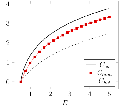
Figure 1: Classical capacities of the optical measurement channels

According to the corollary 1, the relation (33) holds for arbitrary pure measurement channel including heterodyne channel, which maps a density operator $S$ into probability density $\langle x,y|S|x,y\rangle$ with respect to the Lebesgue measure on the plane, where $|x,y\rangle$ are the coherent states of the quantum oscillator [4]. Notice that in this case the bounded operator density exists and results of paper [10] are applicable. The classical capacity of the heterodyne channel computed in  [13], [4] is equal to

$$C(\mathcal{M}_{\rm het},{\mathcal{A}}_{E})=\log\bigg{(}E+\frac{1}{2}\bigg{)}.$$ (35)

For all $E>1/2$ the inequalities hold

$$C(\mathcal{M}_{\rm het},{\mathcal{A}}_{E})<C(\mathcal{M}_{\rm hom},{\mathcal{A}}_{E})<C_{\rm ea}(\mathcal{M},{\mathcal{A}}_{E}).$$

The graphs of the three capacities are shown on Fig. 1.

References

[1]Bennett C. H., Shor P. W., Smolin J. A., Thapliyal A. V. Entanglement-assisted capacity of a quantum channel and the
reverse Shannon theorem. — IEEE Trans. Inform. Theory, 2002, v. 48, No 10, p. 2637–2655.
[2]Berta M., Renes J. M., Wilde M. M. Identifying the information gain of a quantum measurement.
arXiv:1301.1594.
[3]Holevo A. S. The classical capacities of quantum channel
with input constraint. — Theory Probab. Appl., 2004,
v. 48, No 2, p. 243 255.
[4]Holevo A. S. Information capacity of quantum observable. — Problems Inform. Transmission, 2012, v. 48, No 1, p. 1–10 .
[5]Dobrushin R. L. General formulation of Shannon theorem
in information theory. — Russian Math. Surveys, 1959, v. 14, No 6,
p. 3–104.
[6]Holevo A. S. Entanglement-breaking channels in infinite dimensions.
— Problems Inform. Transmission, 2008, v. 44, No 3, p. 171 -184 .
[7]Shirokov M. E. Entropy reduction of
quantum measurement. — J. Math. Phys., 2011, v. 52, No 5, paper No 052202, 18 p.
[8]Holevo A. S. Quantum systems, channels, information. .: , 2010, 327 .
[9]Barchielli A., Lupieri G. Instruments and
mutual entropies in quantum information. — Banach Center Publ., 2006, v. 73, p. 65–80.
[10]Kuznetsova A. A., Holevo A. S. Coding theorems for hybrid channels.
— Theory Probab. Appl., 2013, v. 58, No 2, p. 298–324.
[11]Lindblad G. Expectations and entropy inequalities for finite quantum systems. — Comm. Math. Phys., 1974, v. 39, p. 111–119.
[12]Caves C. M., Drummond P. B.
Quantum limits of bosonic communication rates. — Rev. Modern Phys., 1994, v. 66, p. 481–538.
[13]Hall M. J. W. Quantum information and correlation
bounds. — Phys. Rev. A, 1997, v. 55, No 1, p. 100–113.