Mixed quantal-semiquantal dynamics with stochastic particles for backreaction

Abstract

A mixed quantal-semiquantal theory is presented in which the semiquantal squeezed-state wave packet describes the heavy degrees of freedom. We first derive mean-field equations of motion from the time-dependent variational principle. Then, in order to take into account the interparticle correlation, in particular the ‘quantum backreaction’ beyond the mean-field approximation, we introduce the stochastic particle description for both the quantal and semiquantal parts. A numerical application on a model of O₂ scattering from a Pt surface demonstrates that the proposed scheme gives correct asymptotic behavior of the scattering probability, with improvement over the mixed quantum-classical scheme with Bohmian particles, which is comprehended by comparing the Bohmian and the stochastic trajectories.

Mixed quantum-classical (MQC) dynamics have been a subject of interest not only in chemical physics Pechukas (1969); Meyer and Miller (1979); Bittner and Rossky (1995); Micha (1996); Martens and Fang (1997); Sholl and Tully (1998); Kapral and Ciccotti (1999); Thoss and Stock (1999); Gindensperger et al. (2000); Prezhdo and Brooksby (2001); Deumens and Öhrn (2001); Ando and Santer (2003); Burghardt and Parlant (2004) but also in quantum gravity Anderson (1995); Halliwell (1998), cosmology Hu and Sinha (1995); Campos and Verdaguer (1997), and measurement Machida and Namiki (1980); Zurek (2003). One major problem lies in the description of correlation between the two parts, in particular, the force from the delocalized quantal part to the localized classical part, that is, the problem of ‘quantum backreaction’. It is intimately related to the description of non-adiabatic transitions in which the Born-Oppenheimer approximation breaks down, for instance, near the conical intersections of adiabatic states. Many theories have been proposed, but the problem is inherently of approximate nature Terno (2006); Salcedo (2012). Thus, the assessment would be based not only on the theoretical consistency but also on the practical accuracy in applications. In addition, simplicity for computational implementation to realistic systems will be an important aspect.

In chemical physics, the quantum part usually represents electrons or protons, and the classical part represents heavier nuclei. For the latter, localized wave packet (WP) description, typically by Gaussian WPs Heller (1976); Littlejohn (1986), is also useful. In recent years, we have been studying a ‘semiquantal’ (SQ) squeezed-state WP theory for chemical problems, with applications to hydrogen-bond structure and dynamics Ando (2004, 2005, 2006); Sakumichi and Ando (2008); Hyeon-Deuk and Ando (2009, 2010); Ono and Ando (2012); Ono et al. (2013). An extension to electron WPs with the valence-bond spin-couplings was also examined Ando (2009, 2012), and a combination of nuclear and electron WPs was applied to liquid hydrogen Hyeon-Deuk and Ando (2012, 2014). Following these, we put forward in this Letter a mixed quantal-semiquantal (MQSQ) theory.

We start with a trial wave function and derive the equations of motion (EOM) by the time-dependent variational principle. The resulting EOM for the SQ part have the canonical Hamiltonian form for the center and width variables of the WP. The quantal part follows a time-dependent Schrödinger equation (TDSE), in which the potential energy function is averaged over the SQ WP and thus includes the WP variables as the time-dependent external parameters. The potential function for the evolution of the SQ part is an average over both the SQ WP and quantal wave function, and thus we encounter the problem of ‘backreaction’. To address this, we propose in this work to exploit the theory of stochastic particle (SP) dynamics Nelson (1966); Yasue (1981). The SP dynamics are described by the stochastic differential equations (SDE) whose Fokker-Planck form is equivalent to the TDSE. We thus describe both the quantal and SQ wavefunctions by the corresponding sets of SPs. By assuming the pre-averaged form for the interaction between the SPs, the interparticle correlation beyond the mean-field approximation is described.

The coordinates of the quantal and SQ parts are represented by $x$ and $X$. For simplicity, we consider the SQ WP of the form Arickx et al. (1986); Tsue (1992); Pattanayak and Schieve (1994)

$$\chi_{\Gamma}(X,t)=N_{t}\exp\left[-\left(\frac{1}{4\rho_{t}^{2}}-\frac{i}{\hbar}\frac{\Pi_{t}}{2\rho_{t}}\right)\left(X-Q_{t}\right)^{2}\right.\\ \left.+\frac{i}{\hbar}P_{t}\left(X-Q_{t}\right)\right],$$ (1)

in which $N_{t}=1/(2\pi\rho_{t}^{2})^{1/4}$. The WP is characterized by a set of time-dependent variables $\Gamma_{t}\equiv\{Q_{t},P_{t},\rho_{t},\Pi_{t}\}$, where $Q_{t}$ and $\rho_{t}$ describe the WP center and width, $P_{t}$ and $\Pi_{t}$ are their corresponding conjugate momenta. Generalization to a correlated multi-dimensional WP, in which the variables are vectors and matrices, has been implemented for a simulation of liquid water Ono and Ando (2012), but the simpler form of Eq. (1) would be appropriate for this first presentation.

For the total wave function, we set forth a factorized form

$$\psi_{\gamma\Gamma}\left(x,X,t\right)=\chi_{\Gamma}(X,t)\hskip 1.99997pt\varphi_{\gamma\Gamma}\left(x,t\right).$$ (2)

The idea behind this factorization will be discussed below. The subscript $\Gamma$ indicates the dependence on the variables that characterize the SQ WP of Eq. (1). Similarly, $\gamma$ consists of a set of variables that characterize the quantal wave function $\varphi$; in applications to the electronic wave function, they can be the coefficients of molecular orbitals or configuration interaction, the Thouless parameters for Slater determinant, or the electron WP variables. In some cases, $\varphi$ may also depend parametrically on the SQ WP variables $\Gamma$, as indicated by the subscript to $\varphi$ in Eq. (2). Recently, exact factorization of molecular wave functions to electronic and nuclear parts has been discussed Abedi et al. (2010); Cederbaum (2013). The idea here is rather simple; as we will take into account the interparticle correlation via the combination with the SP description, we start with the factorized form Eq. (2) in a sense to avoid double-counting of the correlation.

The time-dependence of the wave function $\psi_{\Gamma\gamma}$ is described by the variables $\Gamma_{t}$ and $\gamma_{t}$ whose EOM are derived from the time-dependent variational principle with the action integral ${\cal S}=\int_{t_{1}}^{t_{2}}dt\langle\psi(t)|i\hbar\partial_{t}-\hat{H}|\psi(t)\rangle,$ in which

$$\hat{H}=\hat{T}_{\!x}+\hat{T}_{\!X}+v(x,X)$$ (3)

is the Hamiltonian with the kinetic energies $\hat{T}_{\!x}$ and $\hat{T}_{\!X}$ and the potential energy $v(x,X)$. With the trial wave function of Eq. (2), the stationary condition of the action ${\cal S}$ with respect to the variation of $\varphi$, $\delta{\cal S}/\delta\varphi=0$, gives

$$i\hbar\frac{\partial}{\partial t}\varphi_{\gamma\Gamma}\left(x,t\right)=\left(\hat{T}_{\!x}+V\left(x;\Gamma_{t}\right)\right)\varphi_{\gamma\Gamma}\left(x,t\right),$$ (4)

in which $V$ is the averaged potential over the SQ WP $\chi$,

$$V\left(x;\Gamma_{t}\right)=\int dX\left|\chi_{\Gamma}(X,t)\right|^{2}v(x,X).$$ (5)

Equation (4) has a form of TDSE affected by the external time-dependent variables $\Gamma_{t}$ that represent the SQ WP. The variation with respect to the variables in $\chi$, $\delta{\cal S}/\delta\Gamma=0$, gives the EOM of the canonical Hamilton form

$$\dot{Q}=\frac{\partial\tilde{H}}{\partial P},\hskip 5.0pt\dot{P}=-\frac{\partial\tilde{H}}{\partial Q},\hskip 5.0pt\dot{\rho}=\frac{\partial\tilde{H}}{\partial\Pi},\hskip 5.0pt\dot{\Pi}=-\frac{\partial\tilde{H}}{\partial\rho},$$ (6)

with the Hamiltonian in the extended phase-space $\Gamma$,

$$\tilde{H}=\frac{P^{2}}{2M}+\frac{\Pi^{2}}{2M}+\frac{\hbar^{2}}{8M\rho^{2}}+U_{\gamma}(\Gamma),$$ (7)

in which $M$ is the mass for $X$ and

$$U_{\gamma}(\Gamma)=\int dx\left|\varphi_{\gamma\Gamma}(x)\right|^{2}V(x;\Gamma).$$ (8)

In Eq. (5), the SQ coordinate $X$ is integrated to give $V(x;\Gamma)$, whereas in Eq. (8), both $x$ and $X$ are integrated to give $U_{\gamma}(\Gamma)$. Therefore, the dynamics of quantal and SQ parts that follow Eqs. (4)–(7) are under the mutual ‘mean-field’, which causes the problem of describing the ‘backreaction’. To address this, we propose in this work to deploy the theory of SP dynamics Nelson (1966); Yasue (1981). The SP dynamics are described by the SDE,

$$dx_{t}=\frac{\hbar}{m}\left(\nabla_{\!x}S+\nabla_{\!x}R\right)dt+\sqrt{\frac{\hbar}{m}}dW_{t},$$ (9)

in which $m$ is the mass for $x$ and $W_{t}$ represent the standard Wiener process. The SDE for the $X$ part has the analogous form. The functions $R$ and $S$ are the real and imaginary parts of $\ln\psi(x,X,t)=R(x,X,t)+iS(x,X,t).$ For the SQ WP of Eq. (1), the SDE is

$$dX_{t}=\left[\frac{P_{t}}{M}+\frac{\Pi_{t}}{M}\left(\frac{X_{t}-Q_{t}}{\rho_{t}}\right)\right.\\ \left.-\frac{\hbar}{2M\rho_{t}}\left(\frac{X_{t}-Q_{t}}{\rho_{t}}\right)\right]dt+\sqrt{\frac{\hbar}{M}}dW_{t}.$$ (10)

The first two terms in the right-hand-side correspond to the ‘current’ velocity, whereas the third term is the ‘osmotic’ velocity. The first term $P/M$ represents the ordinary velocity of the WP center. The second term describes the breathing velocity of WP width, $\Pi/M$, scaled by a factor $(X-Q)/\rho$, which indicates that the particles in the regions of WP tail move faster than those near the WP center. The third term is also scaled by the same ratio $(X-Q)/\rho$, but has the opposite sign from the second term, and the factor $\hbar/(2M\rho)$ implies its origin from the quantum uncertainty.

Equations (9) and (10) gives the description equivalent to that of the guide wave function $\psi(x,X,t)$. Hence, as long as we employ the original Eqs. (4)–(8), the SPs will still be under the mutual mean-field. Now we propose to replace $V(x;\Gamma)$ in Eq. (4) by the bare $v(x,X)$, and $U_{\gamma}(\Gamma)$ in Eq. (7) by $V(x;\Gamma)$, in an aim to take into account the interparticle correlations. Therefore, the calculation proceeds as follows. (i) We introduce a set of SP pairs $\{(x_{\alpha},X_{\alpha})\}$, $\alpha=1,2,\cdots,N_{\rm sp}$, distributed according to the initial wave function $\psi(x,X,0)$. Each pair $(x_{\alpha},X_{\alpha})$ associates guide wave functions $\varphi_{\alpha}$ and $\chi_{\alpha}$. (ii) We propagate them by

$$i\hbar\frac{\partial}{\partial t}\varphi_{\alpha}\left(x,t\right)=\left(\hat{T}_{\!x}+v\left(x,X_{\alpha}\right)\right)\varphi_{\alpha}\left(x,t\right),$$ (11)

and Eq. (6) with

$$\tilde{H}_{\alpha}=\frac{P_{\alpha}^{2}}{2M}+\frac{\Pi_{\alpha}^{2}}{2M}+\frac{\hbar^{2}}{8M\rho_{\alpha}^{2}}+V(x_{\alpha};\Gamma_{\alpha}),$$ (12)

and $(x_{\alpha},X_{\alpha})$ by the SDEs (9) and (10). This scheme is denoted by MQSQ-SP. The propagation by Eqs. (4)–(8) conserves the total energy expectation $\langle E\rangle=\langle\psi|\hat{H}|\psi\rangle=\langle\varphi|\hat{T}_{x}|\varphi\rangle+\tilde{H}$, but the conservation is lost once the SPs are introduced via Eqs. (11)–(12). In this regard, parallel investigation of these two schemes will be useful in practical studies.

Before proceeding to the numerical application, we note the relation between the MQSQ-SP and the MQC schemes. By the classical point particle approximation for the heavy $X$ part

$$\left|\chi_{\Gamma}(X)\right|^{2}\to\delta(X-Q_{t}),$$ (13)

we find $V(x;\Gamma_{t})\to v(x,Q_{t})$ in Eq. (5), and then $U_{\gamma}(\Gamma)$ in Eq. (8) is replaced by

$$U_{\gamma}(Q)=\int dx\left|\varphi_{\gamma Q}(x)\right|^{2}v(x,Q).$$ (14)

By introducing the Bohmian particles for the quantal $x$ part and replacing the potential energy $U$ by the bare $v(x,X)$, a MQCB scheme analogous to the previous ones Prezhdo and Brooksby (2001); Gindensperger et al. (2000) is obtained. We also note that the present MQSQ-SP has some similarity to the time-dependent quantum Monte-Carlo method Christov (2007). The apparent and most significant difference is in the deployment of SQ WP.

As a numerical demonstration, we study the same model as in Refs. Prezhdo and Brooksby (2001); Sholl and Tully (1998) for gaseous O₂ collision to a Pt surface, a prototype in which the ordinary MQC mean-field (MQC-MF) method fails to describe the temporal splitting of the wave function to trapped and scattered parts. The potential function is given by

$$v(x,X)= \frac{1}{2}M\Omega^{2}X^{2}+a\left[{\rm e}^{-2b(x-c)}-2{\rm e}^{-b(x-c)}\right]$$

$$+A\;{\rm e}^{-B(x-X)}.$$ (15)

The first term is a harmonic binding potential of the heavy particle $X$ to the surface, the second term is a Morse potential for the interaction between the light particle $x$ and the surface, and the third term is a repulsive interaction between the particles. For this $v(x,X)$, the $V$ of Eq. (5) is derived as

$$V(x;\Gamma)= \frac{1}{2}M\Omega^{2}\left(X^{2}+\rho^{2}\right)+a\left[{\rm e}^{-2b(x-c)}-2{\rm e}^{-b(x-c)}\right]$$

$$+A\;{\rm e}^{-B(x-X)+(B\rho)^{2}/2}.$$ (16)

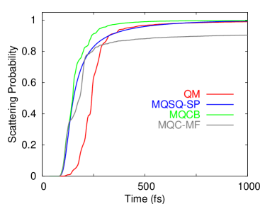
Figure 1: (Color online) Scattering probability from the methods of full quantum mechanics (QM), mixed quantal-semiquantal with stochastic particles (MQSQ-SP), mixed quantum-classical with Bohmian particles (MQCB), and mixed quantum-classical mean-field approximation (MQC-MF).

The initial wave function at $t=0$ is set as a product of the harmonic ground-state wave function for $X$ and a Gaussian WP for $x$ centered at $x=x_{0}$ with a width $\gamma$ and the momentum $k_{0}$,

$$\psi(x,X,0)=N\exp\left[-\frac{M\Omega X^{2}}{2\hbar}\right]\exp\left[-\frac{(x-x_{0})^{2}}{\gamma^{2}}+\frac{ik_{0}x}{\hbar}\right],$$ (17)

in which $N=\left(2M\Omega/\pi^{2}\hbar\gamma^{2}\right)^{1/4}$. The initial momentum $k_{0}$ is specified by the energy $E_{0}$ via $k_{0}=-\sqrt{2mE_{0}}$. We have taken the numerical parameters from Ref. Prezhdo and Brooksby (2001): $m=1$ amu, $M=10$ amu, $\Omega=5\times 10^{14}\textrm{ s}^{-1}$, $A=10^{4}$ kJ/mol, $B=4.25\textrm{ \AA}^{-1}$, $a=700$ kJ/mol, $b=5.0\textrm{ \AA}^{-1}$, $c=0.7$ Å, $x_{0}=6.0$ Å, and $\gamma=0.5$ Å. The quantum mechanical (QM) wave functions were propagated using Cayley’s hybrid scheme with real-space grids Watanabe and Tsukada (2000). Convergence and unitarity of the propagation were confirmed with the grid lengths $\Delta x=0.0178$ Å, $\Delta X=0.0159$ Å, and the time step $\Delta t=0.0124$ fs. The trajectories of ($Q,P$) and ($\rho,\Pi$) conjugate pairs were propagated by Suzuki’s symplectic fourth-order scheme Suzuki (1990). The transmission-free absorbing potential Gonzalez-Lezana et al. (2004) was applied to the scattered wave function along $x$. The results presented are with the absorbing potential set at 81 Å $<x<$ 91 Å, although converged results were obtained with 45 Å $<x<$ 51 Å. For the number of SP pairs, convergence was found with $N_{\rm sp}=2000$. The same number of Bohmian particles were used in the MQCB calculation.

Figure 1 presents the scattering probability defined by

$$P_{\rm s}(t)=\int_{x_{\rm s}}^{\infty}dx\int_{-\infty}^{\infty}dX\;|\psi(x,X,t)|^{2},$$ (18)

with $x_{\rm s}=$ 5.8 Å Sholl and Tully (1998). The MQSQ-SP reproduces the correct asymptotic behavior, in contrast to the MQC-MF and with improvement over the MQCB. However, the description of delayed initial increase of QM $P_{\rm s}(t)$, due to the temporal resonance trapping by the heavy particle excitation Sholl and Tully (1998), was still incomplete. In this regard, an intriguing further test would be to introduce dissipation to the heavy part.

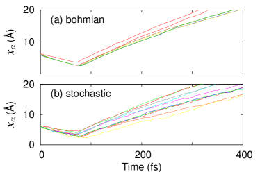
Figure 2: (Color online) Sample (ten) trajectories of (a) Bohmian particles in MQCB and (b) stochastic particles in MQSQ-SP.

In an aim to understand the improved description, we plot in Fig. 2 sample trajectories of stochastic and Bohmian particles. The difference basically emerges from the osmotic term $\nabla R/m$ and the stochastic term $\sqrt{\hbar/m}\;dW$ in Eq. (9); the Bohmian dynamics do not involve them but only the current velocity $dx_{t}=\nabla S/m$. This provides an understanding of the more ballistic trajectories of Bohmian in Fig. 2a. However, further analysis revealed that the use of SPs alone does not account for the difference, because a combination of MQC and SP resulted in $P_{\rm s}(t)$ almost identical to that from MQCB, which indicates that the combination of MQSQ and SP is essential for the result in Fig. 1.

In summary, we have formulated a MQSQ theory with a SP description of the interparticle correlation, and examined it numerically for a prototype model involving wave function splitting. Despit its simplicity, the results were encouraging, although a need for refining the description of interparticle correlation was still evident. We also note that the model employs for the heavy part a harmonic potential on which classical mechanics is patently appropriate. More stringent tests should clarify the nature of the present MQSQ scheme. Particularly interesting would be the cases in which the quantum mechanical aspects of the heavy part play some role, for instance, in the zero-point energy leakage Habershon and Manolopoulos (2009).

Finally, we note that the SQ WP of Eq. (1) can be regarded as a coherent state basis for the path-integral formulation of quantum propagator Kuratsuji (1981). We have recently demonstrated that the initial value representation of the propagator in combination with the SQ WP is applicable Ando (2014). This will provide more flexible description of the wave function by the proper inclusion of quantum phase. Its integration with the present MQSQ formulation is a direction in which to proceed.

The author acknowledges support from KAKENHI Nos. 22550012 and 26620007.

References

- Pechukas (1969) P. Pechukas, Phys. Rev. 181, 166 (1969).
- Meyer and Miller (1979) H. D. Meyer and W. H. Miller, J. Chem. Phys. 70, 3214 (1979).
- Bittner and Rossky (1995) E. R. Bittner and P. J. Rossky, J. Chem. Phys. 103, 8130 (1995).
- Micha (1996) D. A. Micha, Int. J. Quant. Chem. 60, 109 (1996).
- Martens and Fang (1997) C. C. Martens and J. Y. Fang, J. Chem. Phys. 106, 4918 (1997).
- Sholl and Tully (1998) D. S. Sholl and J. C. Tully, J. Chem. Phys. 109, 7702 (1998).
- Kapral and Ciccotti (1999) R. Kapral and G. Ciccotti, J. Chem. Phys. 110, 8919 (1999).
- Thoss and Stock (1999) M. Thoss and G. Stock, Phys. Rev. A 59, 64 (1999).
- Gindensperger et al. (2000) E. Gindensperger, C. Meier, and J. A. Beswick, J. Chem. Phys. 113, 9369 (2000).
- Prezhdo and Brooksby (2001) O. V. Prezhdo and C. Brooksby, Phys. Rev. Lett. 86, 3215 (2001).
- Deumens and Öhrn (2001) E. Deumens and Y. Öhrn, J. Phys. Chem. A 105, 2660 (2001).
- Ando and Santer (2003) K. Ando and M. Santer, J. Chem. Phys. 118, 10399 (2003).
- Burghardt and Parlant (2004) I. Burghardt and G. Parlant, J. Chem. Phys. 120, 3055 (2004).
- Anderson (1995) A. Anderson, Phys. Rev. Lett. 74, 621 (1995).
- Halliwell (1998) J. J. Halliwell, Phys. Rev. D 57, 2337 (1998).
- Hu and Sinha (1995) B. L. Hu and S. Sinha, Phys. Rev. D 51, 1587 (1995).
- Campos and Verdaguer (1997) A. Campos and E. Verdaguer, 36, 2525 (1997).
- Machida and Namiki (1980) S. Machida and M. Namiki, Prog. Theor. Phys. 63, 1833 (1980).
- Zurek (2003) W. H. Zurek, Rev. Mod. Phys. 75, 715 (2003).
- Terno (2006) D. R. Terno, Found. Phys. 36, 102 (2006).
- Salcedo (2012) L. L. Salcedo, Phys. Rev. A 85, 022127 (2012).
- Heller (1976) E. J. Heller, J. Chem. Phys. 64, 63 (1976).
- Littlejohn (1986) R. G. Littlejohn, Phys. Rep. 138, 193 (1986).
- Ando (2004) K. Ando, J. Chem. Phys. 121, 7136 (2004).
- Ando (2005) K. Ando, Phys. Rev. B 72, 172104 (2005).
- Ando (2006) K. Ando, J. Chem. Phys. 125, 014104 (2006).
- Sakumichi and Ando (2008) N. Sakumichi and K. Ando, J. Chem. Phys. 128, 164516 (2008).
- Hyeon-Deuk and Ando (2009) K. Hyeon-Deuk and K. Ando, J. Chem. Phys. 131, 064501 (2009).
- Hyeon-Deuk and Ando (2010) K. Hyeon-Deuk and K. Ando, J. Chem. Phys. 132, 164507 (2010).
- Ono and Ando (2012) J. Ono and K. Ando, J. Chem. Phys. 137, 174503 (2012).
- Ono et al. (2013) J. Ono, K. Hyeon-Deuk, and K. Ando, Int. J. Quant. Chem. 113, 356 (2013).
- Ando (2009) K. Ando, Bull. Chem. Soc. Jpn. 82, 975 (2009).
- Ando (2012) K. Ando, Chem. Phys. Lett. 523, 134 (2012).
- Hyeon-Deuk and Ando (2012) K. Hyeon-Deuk and K. Ando, Chem. Phys. Lett. 532, 124 (2012).
- Hyeon-Deuk and Ando (2014) K. Hyeon-Deuk and K. Ando, J. Chem. Phys. 140, 171101 (2014).
- Nelson (1966) E. Nelson, Phys. Rev. 150, 1079 (1966).
- Yasue (1981) K. Yasue, J. Funct. Anal. 41, 327 (1981).
- Arickx et al. (1986) F. Arickx, J. Broeckhove, E. Kesteloot, L. Lathouwers, and P. van Leuven, Chem. Phys. Lett. 128, 310 (1986).
- Tsue (1992) Y. Tsue, Prog. Theor. Phys. 88, 911 (1992).
- Pattanayak and Schieve (1994) A. K. Pattanayak and W. C. Schieve, Phys. Rev. E 50, 3601 (1994).
- Abedi et al. (2010) A. Abedi, N. T. Maitra, and E. K. U. Gross, Phys. Rev. Lett. 105, 123002 (2010).
- Cederbaum (2013) L. S. Cederbaum, J. Chem. Phys. 138, 224110 (2013).
- Christov (2007) I. P. Christov, J. Chem. Phys. 127, 134110 (2007).
- Watanabe and Tsukada (2000) N. Watanabe and M. Tsukada, Phys. Rev. E 62, 2914 (2000).
- Suzuki (1990) M. Suzuki, Phys. Lett. A 146, 319 (1990).
- Gonzalez-Lezana et al. (2004) T. Gonzalez-Lezana, E. J. Rackham, and D. E. Manolopoulos, J. Chem. Phys. 120, 2247 (2004).
- Habershon and Manolopoulos (2009) S. Habershon and D. E. Manolopoulos, J. Chem. Phys. 131, 174108 (2009).
- Kuratsuji (1981) H. Kuratsuji, Prog. Theor. Phys. 65, 224 (1981).
- Ando (2014) K. Ando, Chem. Phys. Lett. 591, 179 (2014).