Linear-algebraic bath transformation for simulating complex open quantum systems

Abstract

In studying open quantum systems, the environment is often approximated as a collection of non-interacting harmonic oscillators, a configuration also known as the star-bath model. It is also well known that the star-bath can be transformed into a nearest-neighbor interacting chain of oscillators. The chain-bath model has been widely used in renormalization group approaches. The transformation can be obtained by recursion relations or orthogonal polynomials. Based on a simple linear algebraic approach, we propose a bath partition strategy to reduce the system-bath coupling strength. As a result, the non-interacting star-bath is transformed into a set of weakly-coupled multiple parallel chains. The transformed bath model allows complex problems to be practically implemented on quantum simulators, and it can also be employed in various numerical simulations of open quantum dynamics.

I Introduction

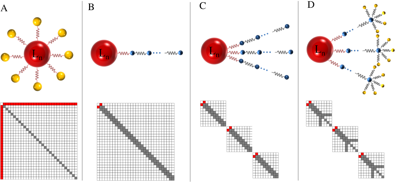
Figure 1: Top panels: Various harmonic oscillator bath models. The red spheres represent system operators and the couplings are shown as springs. The couplings of primary modes, which are directly coupled to the system, are indicated in red. The yellow and blue spheres represent bath oscillators. A. Star-bath model: non-interacting quantum harmonic oscillators (yellow) are coupled to a system operator (red). B. Chain-bath model: a system operator (red) is coupled to a single interacting bath oscillator chain (blue). C. Multiple-chain-bath model: a system operator (red) is coupled to multiple interacting bath oscillator chains (blue). D. Star-chain bath model: a system operator (red) is coupled to multiple chains of bath operators (blue) and final bath oscillators are coupled to non-interacting bath oscillators (yellow). Down panels: The matrix representations (Eq. 6) are shown for the corresponding top panel diagrams. The primary mode couplings to the system are given in red squares and other non-zero elements are shown in gray squares. The first column and row of each matrix correspond to the primary system-bath couplings. The diagonal elements, except the first one, are the frequencies of the bath oscillators.

Problems associated with open quantum systems are of interest in various research fields Breuer and Petruccione (2006). In the theory of open quantum systems, the universe is partitioned into system and bath components. The system of interest is then coupled to the bath degrees of freedom (DOF) by means of an effective Hamiltonian. Solving the full quantum dynamics with currently known exact analytic or numerical methods are not feasible as the system and bath DOF increase. A simple but effective approach to model these vibrations is to treat them as a collection of non-interacting quantum harmonic oscillators bilinearly coupled to the system Breuer and Petruccione (2006); May and Kühn (2011). The system-bath interaction is then characterized by a spectral density function (SDF) that represents the coupling strength in the frequency domain Breuer and Petruccione (2006); May and Kühn (2011). The energy transfer in photosynthetic systems is an example of a complex open quantum system, where the pigments involved in the energy transfer interact with a richly-structured set of molecular vibrations, and hence a very structured SDF van Amerongen et al. (2000).

The spin-boson model Breuer and Petruccione (2006) is one of the simplest models for studying the dynamics of open quantum systems. In the most common representation, the spin-boson model is mathematically represented as a set of non-interacting oscillators coupled to the system. This can be graphically-represented in a star configuration as shown in Fig. 1A Bulla et al. (2003, 2005). Generalized spin-boson models, such as the Hubbard-Holstein model, have been successfully employed to describe the energy transfer process in photosynthetic antenna complexes Huh et al. (2014). Some numerically-exact methods have been so far developed to solve these models, see, for example; reduced-density-matrix approaches, such as hierarchy equations of motion (HEOM) Ishizaki and Tanimura (2005); Ishizaki and Fleming (2009); Kreisbeck et al. (2011), stochastic approaches Strunz and Gisin (1999); Lacroix (2008); Li et al. (2011); Orth et al. (2013), multi-configuration time-dependent Hartree Wang and Thoss (2008), numerical renormalization group (NRG) Bulla et al. (2003, 2005); Schollwöck (2005); Bulla et al. (2008); Prior et al. (2010); Chin et al. (2011), and path-integral approaches Nalbach et al. (2011), amongst many others. However, the applicability of numerically-exact methods is limited by the system size and the bath DOF. For example, the simulation of HEOM with current computers is limited to $\approx$40 sites of the system with only a single Drude-Lorentzian peak representing the bath Kreisbeck et al. (2011); Mostame et al. . In the other hand, the renormalization group approach Schollwöck (2005); Chin et al. (2010, 2011) could be used for relatively large systems. However, the system and bath size that can be handled is still far from that required for solving problems at biological scales. In this approach, then the bath transformation from the non-interacting bath model (Fig. 1A) to the 1-D Wilson chain (Fig. 1B) Wilson (1975) is necessary. The collective modes of the bath oscillators in the chain model has been used widely in various fields such as quantum molecular dynamics Garg et al. (1985); Tretiak et al. (1996), open quantum dynamics Mori (1965); Dupuis (1967); Grigolini and Parravicini (1982); Burghardt et al. (2012); Chenel et al. (2014), quantum information Skinner and Hu (2008) and nuclear physics Iachello and Arima (1987); Caprio (2005).

Quantum simulators defined as controlled quantum devices that can effectively reproduce the dynamics of any other quantum system Feynman (1982, 1986); Lloyd (1996); Buluta and Nori (2009) could become an attractive alternative for solving the dynamics of open quantum systems ”directly”. Different platforms can be used for implementing quantum simulators, such as superconducting qubits Skinner and Hu (2008); Houck et al. (2012); Mostame et al. (2012); Ballester et al. (2012); Mei et al. (2013); Heras et al. (2014); Stojanović et al. (2014); Mostame et al. ; Roushan and et al. (2014), trapped ions Cirac and Zoller (2000); Schützhold et al. (2007); Gerritsma et al. (2011); Casanova et al. (2011a, b, 2012); Blatt and Roos (2012); Stojanović et al. (2012); Schindler et al. (2013), quantum optics Lanyon et al. (2010); Szpak and Schützhold (2011); Herrera and Krems (2011); Aspuru-Guzik and Walther (2012); Bloch et al. (2012), nuclear magnetic resonance (NMR) Du et al. (2010); Lu et al. (2011); Li et al. (2011); Zhang et al. (2011); Feng et al. (2013) or a system of electrons Schützhold and Mostame (2005); Mostame and Schützhold (2008).

The experimental implementation of quantum simulators of open quantum system dynamics, for example, using superconducting circuits Mostame et al. (2012, ), poses challenges due to at least two of the main current constraints in the realizable circuits. First, the number of quantum bath oscillators, that are directly coupled to a system operator (qubit), is limited by the physical size of the superconducting loop that embodies the qubit. Hence, a star-model approach with many oscillators coupled to the qubit may pose fabrication challenges. A physical layout that involves less oscillators directly coupled to a qubit is more experimentally realizable Mostame et al. (2012). In addition, the coupling strength of the qubit to the bath may be limited. In superconducting qubits, the system-bath coupling strength should not exceed a certain percentage of the frequency of the quantum oscillator Mostame et al. .

In this work, we address the question of how the two mentioned implementation issues can be resolved by a unitary bath transformation which introduces interaction terms among the transformed quantum oscillators. In chain-like bath models (Fig. 1B)  Chernyak and Mukamel (1996); Chou et al. (2008); Skinner and Hu (2008); Bulla et al. (2003, 2005); Chin et al. (2010); Prior et al. (2010); Burghardt et al. (2012); Chenel et al. (2014), only one bath oscillator is directly coupled to the system. However, in some cases, one needs to couple more than a single chain to deal with the limitation of the oscillator-qubit coupling mentioned above. Here, we propose a partitioning strategy of the bath modes for multiple parallel chains to reduce primary mode coupling strengths and also the number of the modes directly coupled to the system operator. This is shown in Figs. 1C and D respectively. We found that the coupling strength of the primary modes, which are directly coupled to the system, can be reduced as we increase the number of the chains; at the same time, we can also shorten the lengths of each chain. In addition to the fabrication and implementation benefits for open quantum simulators using quantum hardware, these methods are also potentially applicable to simulations in classical computers. In this case, perturbative methods may be employed to simulate these chain models with reduced system-bath coupling Burghardt et al. (2012); Chenel et al. (2014).

A recurrence equation derived by Bulla et al. Bulla et al. (2005) has been used in the renormalization group approaches to construct the 1-D Wilson chain (Fig. 1B). This recurrence relation, however, potentially shows numerical instabilities Vojta et al. (2005); Bulla et al. (2005, 2008). Recently, Chin et al. Chin et al. (2010) developed an exact mapping approach for a continuous SDF using orthogonal polynomials without discretizing the SDF. However, this approach may pose challenges applicable to arbitrary structured SDFs. In many applications of chemistry and biology, structured SDFs appear when atomistic details are involved in open quantum dynamics, as already mentioned in the introduction. Therefore, the SDFs may not be well approximated as simple analytic functions such as Ohmic spectral functions.

In this paper, we test a generalized linear algebraic transformation approach for any given discrete SDFs, where a transformation on multiple parallel chains is involved, as shown in Fig. 1C. With the multiple chain-bath transformation described in the following sections, complex open quantum systems, such as photosynthetic antennae, can be studied practically via quantum simulators.

In the next sections we present the model Hamiltonian and the linear algebraic bath transformation. As an example, a two-oscillator bath transformation is presented analytically. This example shares many features of our general scheme of bath partitioning. Numerical stability of the bath transformation methods is discussed in the result section and the results are compared with Bulla’s transformation approach Bulla et al. (2005). Then, we propose a way to partition the bath modes into multiple parallel chains to reduce the system-bath coupling strengths. We apply the proposed leaping partitioning (LP) strategy to a structured spectral density of the chlorosome Fujita et al. (2012, 2014), as an example. The numerical result is compared with a ’standard’ sequential partitioning (SP) scheme.

II Chain bath transformation

As mentioned in the introduction, in the theory of open quantum systems, the system-bath Hamiltonian $\hat{H}$ is composed of three parts, namely,

$$\hat{H}=\hat{H}_{\mathrm{S}}+\hat{H}_{\mathrm{SB}}+\hat{H}_{\mathrm{B}}\ ,$$ (1)

where $\hat{H}_{\mathrm{S}}$ is the system Hamiltonian. The phonon bath $\hat{H}_{\mathrm{B}}$ is approximated as a set of non-interacting harmonic oscillators. The coupling term $\hat{H}_{\mathrm{SB}}$ between the system and bath is almost universally treated as a bilinear coupling. More precisely, we write $\hat{H}_{\mathrm{SB}}+\hat{H}_{\mathrm{B}}$ in a compact form Guo (2012) as follows,

$$\hat{H}_{\mathrm{SB}}+\hat{H}_{\mathrm{B}}=\sum_{n}\begin{pmatrix}\hat{L}_{n}&\bm{\hat{a}}_{n}^{\dagger}\end{pmatrix}\mathbf{\Gamma}_{n}\begin{pmatrix}\hat{L}_{n}\\ \bm{\hat{a}}_{n}\end{pmatrix},$$ (2)

$$\mathbf{\Gamma}_{n}=\begin{pmatrix}0&\bm{\kappa}^{\mathrm{t}}_{n}\\ \bm{\kappa}_{n}&\mathbf{\Omega}_{n}\end{pmatrix},$$ (3)

where each creation (annihilation) operator vector $\bm{\hat{a}}_{n}^{\dagger}\,\,(\bm{\hat{a}}_{n})$ of oscillators for the site $n$ are coupled to the operator $\hat{L}_{n}$ that acts on the system. Lower case bold and capital bold fonts are used for a column vector and a matrix, respectively. The bosonic operators satisfy a commutation relation, $[\hat{a}_{n;i},\hat{a}_{m;j}^{\dagger}]=\delta_{nm}\delta_{ij}$ where $\bm{\hat{a}}_{n}=(\hat{a}_{n;1},\ldots,\hat{a}_{n;N})^{\mathrm{t}}$. Here $\mathbf{\Omega}_{n}$ is a diagonal matrix, which has the harmonic frequencies as the elements, i.e. $\mathbf{\Omega}_{n}=\mathrm{diag}(\omega_{n;1},\ldots,\omega_{n;N})$. $\bm{\kappa}_{n}$ is the system-bath coupling strength vector. Accordingly, the SDF $J_{n}(\omega)$ is defined Valleau et al. (2012) as,

$$J_{n}(\omega)=\pi\sum_{j}\kappa_{n;j}^{2}\,\delta(\omega-\omega_{n;j})\ .$$ (4)

The non-interacting bath in Eq. 2 is the star-bath model (Fig. 1A), where the independent harmonic oscillators are all coupled directly to the system.

II.1 Linear algebraic bath transformation

With a suitable choice of unitary transformation on the bath oscillators, one can turn a star-bath into a multiple-chain bath. The multiple-chain bath has a few primary bath oscillators and the remaining oscillators (secondary bath modes) are coupled to the primary bath modes in a chain as depicted in Fig. 1C. A mixture of star and chain models is also possible as shown in Fig. 1D. Burghardt et al. Hughes et al. (2009); Burghardt et al. (2012); Chenel et al. (2014) exploited the latter model to develop a perturbative truncated bath model, which approximates the terminal star-coupled yellow oscillators in Fig. 1D as Markovian baths.

The bath transformation from the star model (Eq. 2) to the 1-D Wilson chain (Fig. 1B) can be simply obtained by a unitary transformation of the matrix $\mathbf{\Gamma}_{n}$ that keeps the system operators unchanged. We introduce, here, an arbitrary unitary transformation ($\mathbf{U}_{n}\mathbf{U}_{n}^{\dagger}=\mathbf{I}$) satisfying the following conditions;

$$\hat{H}_{\mathrm{SB}}+\hat{H}_{\mathrm{B}}=\sum_{n}\begin{pmatrix}\hat{L}_{n}&\bm{\hat{b}}_{n}^{\dagger}\end{pmatrix}\mathbf{\tilde{\Gamma}}_{n}\begin{pmatrix}\hat{L}_{n}\\ \bm{\hat{b}}_{n}\end{pmatrix},$$ (5)

$$\mathbf{\tilde{\Gamma}}_{n}=\begin{pmatrix}0&\bm{\tilde{\kappa}}^{\mathrm{t}}_{n}\\ \bm{\tilde{\kappa}}_{n}&\mathbf{\tilde{\Omega}}_{n}\end{pmatrix}=\begin{pmatrix}1&\bm{0}^{\mathrm{t}}\\ \bm{0}&\mathbf{U}_{n}^{\dagger}\end{pmatrix}\mathbf{\Gamma}_{n}\begin{pmatrix}1&\bm{0}^{\mathrm{t}}\\ \bm{0}&\mathbf{U}_{n}\end{pmatrix},$$ (6)

where $\bm{\hat{b}}_{n}=\mathbf{U}_{n}^{\dagger}\bm{\hat{a}}_{n}$. The first column of $\mathbf{U}_{n}$ is $||\bm{\kappa}_{n}||^{-1}_{2}\bm{\kappa}_{n}$ and the remaining columns are constructed using the Gram-Schmidt process with random vectors (or unit vectors) Golub and Van Loan (1996). As a result, $\mathbf{\tilde{\Gamma}}_{n}$ is a dense symmetric matrix and $\bm{\tilde{\kappa}}_{n}=(\tilde{\kappa}_{n;1},0,\ldots,0)^{\mathrm{t}}$ is the new system-bath coupling strength vector. (see Appendix A for the details and down panels of Fig. 1 for the structures of $\mathbf{\tilde{\Gamma}}_{n}$.)

Now we have new sets of interacting harmonic oscillators while the system operators remain unchanged. The tridiagonalization of $\mathbf{\Gamma}_{n}$ in Eq. 2 for the Wilson chain (Fig. 1B) can be performed numerically by Householder or Lanczos procedures Golub and Van Loan (1996). Alternatively, we use here tridiagonalization of $\mathbf{\tilde{\Omega}}_{n}$, i.e. $\mathbf{\tilde{\Omega}}_{n}=\mathbf{T}\mathbf{\Xi}\mathbf{T}^{\dagger}$, with a Hessenberg reduction of a symmetric matrix Golub and Van Loan (1996). We call the later transformation method as Gram-Schmidt-Hessenberg (GSH). The Hessenberg reduction of a symmetric matrix produces a tridiagonal matrix and then the numerical procedures for the reduction, such as, Householder, Lanczos and Gauss transform, can be applied. These numerical algorithms are standard numerical linear algebraic techniques, see e.g. Ref. Golub and Van Loan (1996).

II.2 Multiple chain transformation

In this subsection we explain the multiple parallel chain transformation that is depicted in Fig. 1C. We introduce a unitary transformation,

$$\mathbf{\tilde{U}}_{n}=\mathbf{P}_{n}\mathbf{U}_{n}\ ,$$ (7)

that additionally rearranges (using a permutation matrix $\mathbf{P}_{n}$) the non-interacting bath oscillators as multiple groups of several interacting oscillators, i.e. $\bm{\hat{b}}_{n}=\mathbf{\tilde{U}}_{n}^{\dagger}\bm{\hat{a}}_{n}$. The unitary transformation matrix $\mathbf{U}_{n}$ is block diagonal and does not allow the interaction between oscillators from different groups (an example of the rearrangement is given in Appendix B.). We also define the following relations for the unitary transformation;

$$\mathbf{\tilde{\Omega}}_{n}=\mathbf{\tilde{U}}_{n}^{\dagger}\mathbf{\Omega}_{n}\mathbf{\tilde{U}}_{n}\quad\mathrm{and}\quad\bm{\tilde{\kappa}}_{n}=\mathbf{\tilde{U}}_{n}^{\dagger}\bm{\kappa}_{n}\ .$$ (8)

The primary modes, which are directly coupled to the system operators, are defined as collective oscillator modes by choosing the first column of the $l$-th subblock $\mathbf{U}_{n}^{(l)}$ to be $||\bm{g}^{(l)}_{n}||^{-1}_{2}\bm{g}^{(l)}_{n}$. The normalized vector corresponds to the rearranged coupling strength vector of

$$\bm{g}_{n}=\mathbf{P}_{n}^{\dagger}\bm{\kappa}_{n}=\begin{pmatrix}\bm{g}^{(1)}_{n}\\ \vdots\\ \bm{g}^{(N_{eff})}_{n}\end{pmatrix},$$ (9)

with $N_{eff}$ being the number of subblocks (or the number of group of oscillators). The chain-bath model can be obtained via tridiagonalization of $l$-th subblock

$$\mathbf{\tilde{\Omega}}_{n}^{(l)}=\mathbf{T}^{(l)}\mathbf{\Xi}^{(l)}\mathbf{T}^{(l)\dagger}\$$ (10)

with applying the Hessenberg transform Golub and Van Loan (1996) via the Householder procedure. $\mathbf{\Xi}^{(l)}$ is a tridiagonal matrix that defines the frequencies (diagonal elements) of the transformed bath modes and coupling strengths (off-diagonal elements) between the oscillators in the chain model. $\mathbf{T}^{(l)}$ is a Hessenberg unitary transform matrix that makes no transformation to the primary bath mode such that the first column of the matrix is $(1,0,\ldots,0)^{\mathrm{t}}$. The resulting transformed bath coupling vector $\mathbf{T}^{(l)}\bm{\tilde{\kappa}}_{n}^{(l)}$ of the $l$-th subblock has only a single non-zero first element, which corresponds to the primary mode coupling strength. In Appendix C, we provide a MATLAB MATLAB (2013) code for the GSH with the LP scheme.

The alternative numerical transformation from the star-bath model to the chain-bath model can be obtained by Bulla’s recursion method Bulla et al. (2003, 2005). The two methods will be compared numerically later.

III Results and discussion

III.1 Numerical stability of the transformations

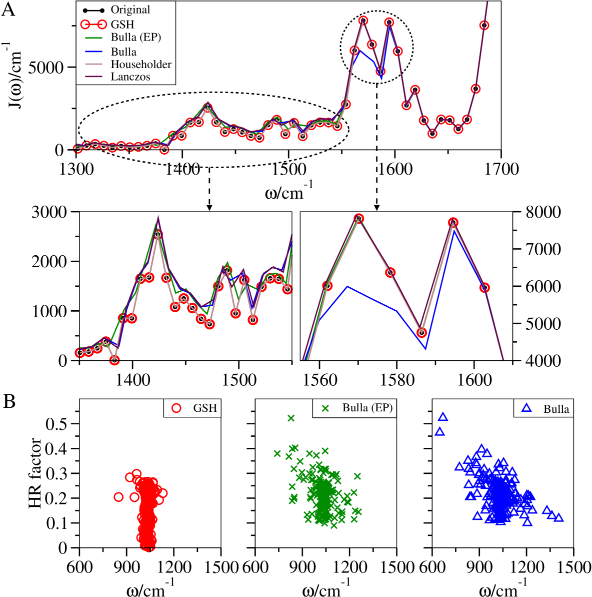
Figure 2: Reconstructed spectral densities of the chlorosome from a chain bath. A. Reconstructed spectral densities of chlorosome from different numerical transformations are compared with the original one. B. Huang-Rhys (HR) factors of the secondary bath oscillators with nearest-neighbor couplings in a single chain model. Two different unitary mapping methods are compared. Red circles are calculated by the Gram-Schmidt-Hessenberg (GSH) transform. Green crosses and blue triangles are obtained from Bulla’s method Bulla et al. (2005) with and without the extended precision (EP), respectively.

To test the numerical stability of the 1-D Wilson chain transformation methods, we perform back transformations from the chain-bath Hamiltonian to the star-bath Hamiltonian (Eq. 2) by a straightforward diagonalization of $\mathbf{\tilde{\Omega}}_{n}$. The structured SDFs are reconstructed by the back transformation and then compared with the original SDF of the chlorosome, as an example system. The chlorosome is a giant light harvesting antenna complex of green sulfur bacteria Blankenship (2002). The excitation energy is transferred within the antenna via the fluctuating environment. Various models were developed to study the system from the open quantum dynamics perspective Fujita et al. (2012, 2014); Huh et al. (2014). Here we use the SDF of the chlorosome that some of us Fujita et al. (2012) obtained via quantum mechanics/molecular mechanics (QM/MM) calculations that contain 253 peaks corresponding to the quantum bath oscillators. In Fig. 2A, only the peaks in 1300–1700 cm^-1 are shown for clarity. The original SDF is plotted as a black line and filled black circles. Bulla’s method (blue line) suffers from numerical instability as the iteration increases. Therefore, we also test extended precision (EP; 100 digits) with Bulla’s method (green line). The GSH curve is shown as a red line and unfilled red circles. Householder and Lanczos transformations of $\mathbf{\Gamma}_{n}$ in Eq. 3 are plotted in brown and purple lines, respectively. As expected, Bulla’s original method generates a curve that deviates significantly from the original one, especially around 1550–1600 cm^-1. The EP improves the result but is still in disagreement with the original. The Lanczos curve seems to agree well with the original but the discrete data points do not match with the original data points in the frequency domain and it produces negative frequencies that are not shown in the figure. The GSH and Householder, on the other hand, can reproduce the original SDF with high accuracy. Both methods are based on the Householder procedure, which has an unconditional stability Businger (1969).

Fig. 2B indicates the Huang-Rhys (HR) factors of secondary bath oscillators with nearest-neighbor couplings in a chain, that are obtained from different methods. The HR factor $\chi_{j}$ of a harmonic oscillator with frequency $\omega_{j}$ is a normalized coupling strength given by $\kappa_{j}=\omega_{j}\sqrt{\chi_{j}}$. For the secondary modes, HR factors are defined with the frequencies of the oscillators and the coupling strengths with the nearest neighbors in the chain. As one compares the results from Bulla’s method (green cross) and Bulla’s method with EP (blue triangle), they are significantly different from each other. This shows that Bulla’s recursion relation is numerically unstable. Comparing the Bulla’s and GSH methods, one can see the Bulla’s method (green cross) produces larger HR factors than the GSH method (red circle). The GSH bath transformation can produce oscillators with frequencies distributed a narrower band. The reason for this difference is that the unitary transformation for the chain model is not unique. Bulla’s method does not allow the secondary bath modes to have negative interactions while the GSH has no such a constraint. Since the unitary matrix for the GSH transform is constructed via orthogonalization of the random vectors, the signs of the interactions in a single chain can vary in each transformation, but their magnitudes are invariant.

III.2 Multiple chain bath model

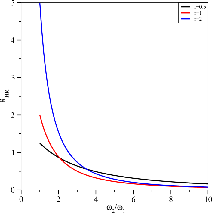
Figure 3: Normalized Huang-Rhys (HR) factor $R_{\mathrm{HR}}$ for the example of bath with two oscillator modes. With selected fixed $f$ values, the normalized HR factors are evaluated at varying the frequency ratio ($\omega_{2}/\omega_{1}$).

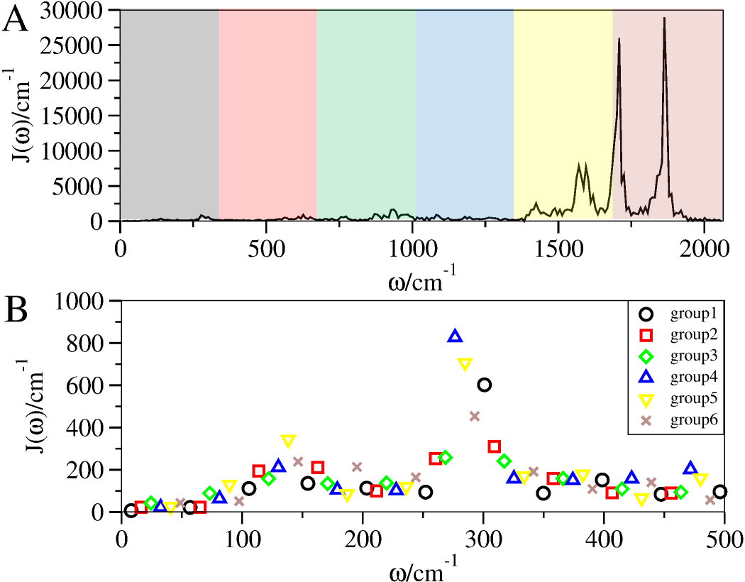
Figure 4: Partitioning schemes of the spectral density function (SDF). A. The sequential partition of the spectral density of chlorosome is depicted. Group of oscillators are indicated with 6 different colors. B. The leaping partition of the spectral density is depicted. The peaks in the spectral density of the chlorosome Fujita et al. (2012, 2014) are partitioned into 6 groups. Only the peaks below 500 cm^-1 are shown for the clarity.

In this subsection, we apply the GSH transformation method to a couple of illustrative examples. First, to get some insights into the weakly-coupled multiple chain model, we employ this method analytically to transform a bath with two oscillator modes. Then, we continue with a multidimensional example of a chlorosome.

In the chain bath model for two oscillators, the mixing of the two modes with frequencies $\omega_{1}\leq\omega_{2}$ leads to a HR factor for the primary mode $\chi_{\mathrm{c}}$:

$$\chi_{\mathrm{c}}=R_{\mathrm{HR}}\chi_{1},$$ (11)

$$R_{\mathrm{HR}}=\frac{(1+f^{2})^{3}}{(1+\tfrac{\omega_{2}}{\omega_{1}}f^{2})^{2}},$$ (12)

where $f=\kappa_{2}/\kappa_{1}$ and $\chi_{1}=\kappa_{1}^{2}/\omega_{1}^{2}$. In Fig. 3, the normalized HR factor $R_{\mathrm{HR}}$ of Eq. 12 is plotted while varying the frequency ratio ($\omega_{2}/\omega_{1}$) at fixed coupling strength ratios $f$, 0.5, 1 and 2. For fixed $f$, the values of $R_{\mathrm{HR}}$ decrease as the frequency ratio increases. $f$ determines the slopes of the curves. Larger $f$ makes the curve decrease faster as $\omega_{2}/\omega_{1}$ increases. When the oscillators have similar frequencies $\omega_{2}/\omega_{1}\simeq 1$, $R_{\mathrm{HR}}$ is larger than 1, which makes the chain bath couplings stronger than the star-bath model. However, as the frequency ratio increases $R_{\mathrm{HR}}$ drops down and it can become arbitrarily small as the frequency difference increases. This gives a hint how to mix the oscillator modes and reduce the coupling strength of the primary modes by forming weakly coupled multiple chains. The oscillators, which have large frequency differences, should be mixed to make the weakly coupled multiple chain bath models.

Next, we apply the GSH method to the example of chlorosome. The SP approach divides the bath oscillators into a sequence of groups of oscillators, as illustrated in Fig. 4A using a different color for each group. Fig. 4B represents the LP scheme, where only the peaks below 500 cm^-1 are shown for the clarity. As indicated here, the oscillators are partitioned into 6 groups to use the LP scheme. In the LP scheme, the elements of the $k$-th group are composed of $k+N_{\mathrm{eff}}j$-th ($\leq N$) modes, where $N_{\mathrm{eff}}$ is the number of groups, $j$ is an integer ($\geq 0$) and $N$ is the total number of oscillators. For example, when one has 10 modes and 3 groups to partition, the SP approach groups modes of (1,2,3), (4,5,6) and (7,8,9,10) as group 1, 2 and 3, respectively. In the other hand, the LP strategy does the partition into (1,4,7,10), (2,5,8) and (3,6,9) for group 1, 2 and 3, respectively.

In Fig. 5, the maximum HR factor and the corresponding coupling strength of the primary modes are plotted by varying the number of chains from 1 to 6. The LP and SP schemes are used for this calculation. The maximum HR factor of the star-bath model is 0.0315. The single chain model has even larger HR factor of the primary mode than the star-bath model for both partitioning schemes. The maximum HR factors from the SP scheme (blue cross) do not decrease as the number of chains increases. The figure shows, however, that the maximum HR factor (black circle) and the corresponding coupling strength (red triangle) decrease as the number of chains increases for the LP scheme. The maximum HR factor from the LP scheme with 6 chains is below 0.01, which corresponds to 10% of the corresponding harmonic frequency. Therefore 6 chains make the chain model suitable for implementation on quantum simulators, since a quantum simulator can have only a few parallel chains and, in addition, the primary mode HR factor is limited. In principle, the values can be reduced further as long as mixing modes is still possible.

The LP and SP schemes are further compared in Fig. 6. This plot shows the HR factor of the primary modes of each chain. The results are indicated in blue crosses and black circles for the SP and LP schemes, respectively. As evidenced by the figure, the LP scheme gives all values below 0.01 while the SP strategy produce bigger values and the maximum value is more than 4 times larger than the LP values. Another important aspect of the LP scheme is that all of the primary HR factors have nearly similar values while the results of the SP scheme deviate largely from each other.

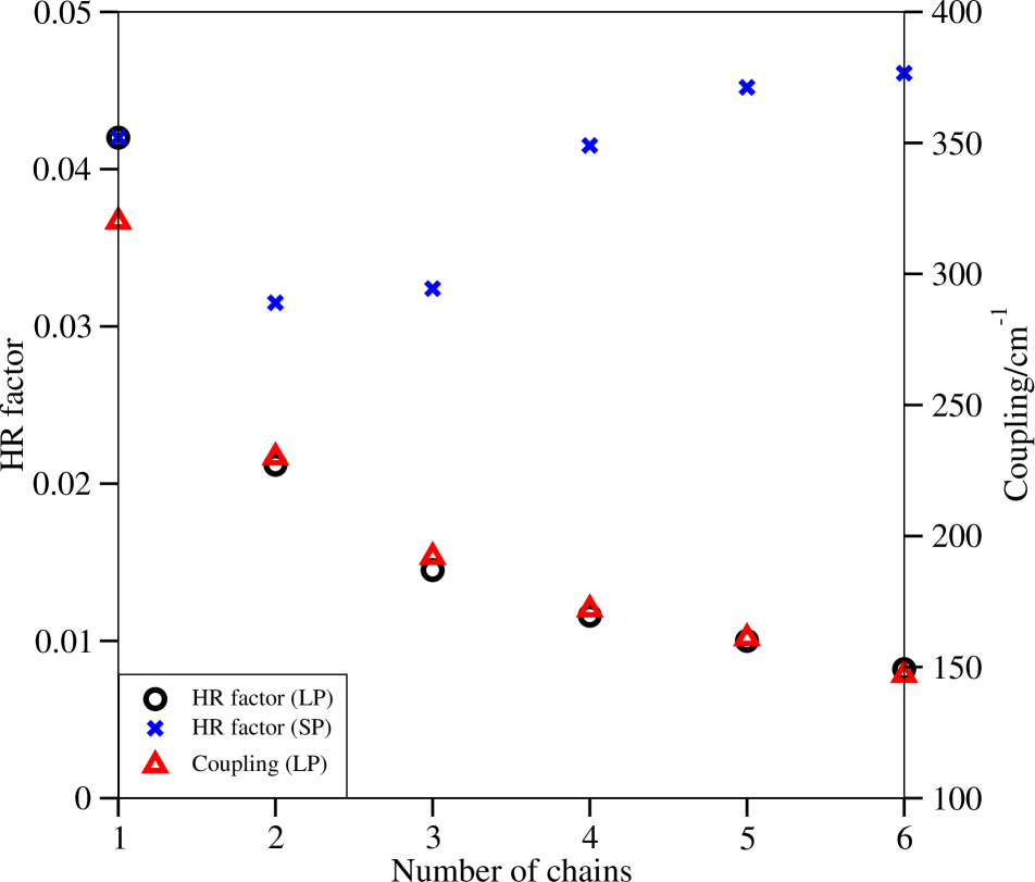
Figure 5: Maximum Huang-Rhys (HR) factor of primary modes of the chlorosome. The maximum HR factor (black circles) of primary modes and the corresponding coupling strengths (red triangles) are plotted as increasing the number of chains for the leaping partitioning (LP) scheme. Blue cross is used for the maximum HR factors from the sequential partitioning (SP) strategy.

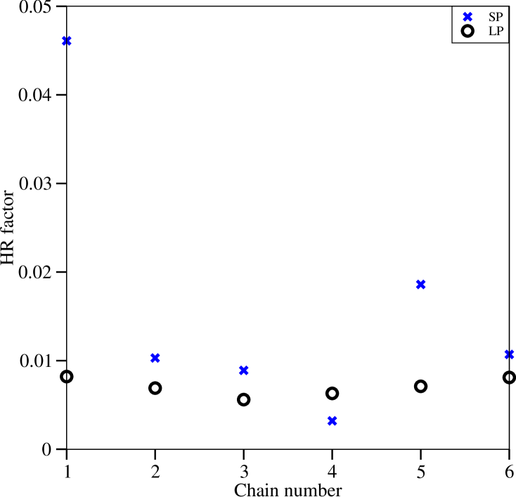
Figure 6: Huang-Rhys (HR) factor of each chain of the chlorosome in different partition schemes. The bath oscillators of chlorosome are transformed to 6 chain bath model with the two different grouping strategies. The sequential partitioning (SP; blue cross) and leaping partitioning (LP; black circle) strategies are compared. Lower HR factors lead to more feasible quantum simulator schemes.

IV Conclusion and outlook

In this paper we show that a multiple chain-bath model, in combination with the leaping bath partitioning scheme, may lead to a practical implementation of quantum simulators for complex open quantum dynamics. We have shown that the multiple chain-bath model can be employed for the realization of quantum simulators for open quantum systems or for numerical studies in classical computers. Furthermore, the leaping partition scheme can reduce the primary mode coupling strength almost homogeneously for all parallel chains. The reason is that the mixing of oscillators with large frequency differences can result in small HR factors. The two-oscillator model was presented with an analytic expression for the chain transformation and provides a hint for the bath partitioning scheme, i.e. leaping partition. We also tested the unitary transformation algorithm that exploits the GSH transformation, and compared the results with the values from Bulla’s recursion method Bulla et al. (2005). The GSH transformation can produce smaller HR factors of the secondary bath modes with oscillators being in a narrower band. The numerical stability of Bulla’s method was discussed and the GSH method was shown to be numerically stable.

Our bath transformation method could be useful for the perturbative approaches as well, because of the resulting weak system-bath couplings. The effective spectral density can be obtained based on the chain-model transformation. It can also be used for the reduced density matrix methods Burghardt et al. (2012); Chenel et al. (2014) for the simulation of non-Markovian dynamics. The effective bath approach with the parallel chain-bath model can also be useful for the HEOM method. The effective bath spectral density can reduce the number of Drude-Lorentzian peaks, then the HEOM method can handle larger systems Mostame et al. . Further work in this direction will be conducted.

Appendix A GSH algorithm

We explain here in details how to construct the unitary transform matrix $\mathbf{U}_{n}$ of GSH transformation in Eq. 6 for $\mathbf{\tilde{\Omega}}_{n}$. A MATLAB MATLAB (2013) script is given in Appendix C.

1. Set the first column of $\mathbf{U}_{n}$ to be the normalized coupling strength vector $||\bm{\kappa}_{n}||^{-1}_{2}\bm{\kappa}_{n}$.
2. Assign random vectors to the remaining columns (from 2 to $N$). We use a normal distribution with the first column to be a mean vector for the random vectors.
3. Perform the Gram-Schmidt orthogonalization to $\mathbf{U}_{n}$.
4. Compute $\mathbf{U}_{n}^{\dagger}\mathbf{\Omega}_{n}\mathbf{U}_{n}$ for $\mathbf{\tilde{\Omega}}_{n}$.

Appendix B Example of permutation matrix

Here we represent a permutation matrix $\mathbf{P}^{\dagger}$, as an example. It permutes a vector of length 4 ($\bm{v}$) to arrange odd and even elements sequentially,

$$\mathbf{P}^{\dagger}\bm{v}=\begin{pmatrix}1&0&0&0\\ 0&0&1&0\\ 0&1&0&0\\ 0&0&0&1\end{pmatrix}\begin{pmatrix}v_{1}\\ v_{2}\\ v_{3}\\ v_{4}\end{pmatrix}=\begin{pmatrix}v_{1}\\ v_{3}\\ v_{2}\\ v_{4}\end{pmatrix}\ .$$ (13)

Appendix C LP scheme with GSH

We provide here a MATLAB MATLAB (2013) script for the LP scheme with the GSH procedure. The script produces a single chain for a subblock, which is assigned by the user. Multiple chains can be obtained by using this script for each subblock. The details of the script can be found in the comments of the script, which are indicated with %.

⬇

1function [HRF,Dn,Xi]=LP(SDF,Sub,Neff)

%-Inputs-

3%SDF: Spectral density function = [frequency spectral-density]

%Sub: Subblock of interest (starting index in the full SDF)

5%Neff: Number of subblocks (index step size for LP scheme)

7%-Outputs-

%HRF: HR factor of the primary mode of the subblock

9%Dn: norm of the coupling vector (equivelent to the coupling strength of the primary mode)

%Xi: Tridiagonal coupling bath coupling matrix

11% Eq. (10), OmegaTilde=T*Xi*T’, T*T’=I

13%Scale SDF with 1/pi

SDF(:,2)=SDF(:,2)/pi;

15%dimension of the SDF

dim=max(size(SDF));

17

%LP scheme for the subgroup

19SDF=spd(Sub:Neff:dim,:);

%new dimension

21dim=max(size(SDF));

23%t1: first column of U, U*U’=I

t1=sqrt(SDF(:,2));

25Dn=norm(t1);

t1=t1/Dn;

27

%Random vectors for the Gram-Schmidt orthogonalization

29%are assigned to columns from 2 to N.

U0=randn(dim,dim-1);

31U0=[t1 U0];

for k=2:dim

33U0(:,k)=U0(:,k)+t1;

end

35%Gram-Schmidt orthogonalization, user should provide the GS routine.

U=GS(U0);

37%OmegaTilde in Eq. 8

OmegaTilde=U’*diag(SDF(:,1))*U;

39%Hessenberg transformation

[T,Xi]=hess(OmegaTilde);

41HRF=Dn^2/Xi(1,1)^2;

43end

References

References

- Breuer and Petruccione (2006) H. P. Breuer and F. Petruccione, The theory of open quantum systems (Oxford University Press, New York, 2006).
- May and Kühn (2011) V. May and O. Kühn, Charge and Energy Transfer Dynamics in Molecular Systems; 3rd ed. (Wiley-VCH, Weinheim, 2011).
- van Amerongen et al. (2000) H. van Amerongen, L. Valkunas, and R. van Grondelle, Photosynthetic excitons (World Scientific, Singapore, 2000).
- Bulla et al. (2003) R. Bulla, N.-H. Tong, and M. Vojta, Phys. Rev. Lett. 91, 170601 (2003).
- Bulla et al. (2005) R. Bulla, H.-J. Lee, N.-H. Tong, and M. Vojta, Phys. Rev. B 71, 045122 (2005).
- Huh et al. (2014) J. Huh, S. K. Saikin, J. C. Brookes, S. Valleau, T. Fujita, and A. Aspuru-Guzik, J. Am. Chem. Soc. 136, 2048 (2014).
- Ishizaki and Tanimura (2005) A. Ishizaki and Y. J. Tanimura, J. Phys. Soc. Jpn. 74, 3131 (2005).
- Ishizaki and Fleming (2009) A. Ishizaki and G. R. Fleming, Proc. Natl. Acad. Sci. 106, 17255 (2009).
- Kreisbeck et al. (2011) C. Kreisbeck, T. Kramer, M. Rodríguez, and B. Hein, J. Chem. Theory Comput. 7, 2166 (2011).
- Strunz and Gisin (1999) W. T. Strunz and N. Gisin, Phys. Rev. Lett. 82, 1801 (1999).
- Lacroix (2008) D. Lacroix, Phys. Rev. E 77, 041126 (2008).
- Li et al. (2011) H. Li, J. Shao, and S. Wang, Phys. Rev. E 84, 051112 (2011).
- Orth et al. (2013) P. P. Orth, A. Imambekov, and K. Le Hur, Phys. Rev. B 87, 014305 (2013).
- Wang and Thoss (2008) H. Wang and M. Thoss, New J. Phys. 10, 115005 (2008).
- Schollwöck (2005) U. Schollwöck, Rev. Mod. Phys. 77, 259–315 (2005).
- Bulla et al. (2008) R. Bulla, T. Costi, and T. Pruschke, Rev. Mod. Phys. 80, 395–450 (2008).
- Prior et al. (2010) J. Prior, A. W. Chin, S. F. Huelga, and M. B. Plenio, Phys. Rev. Lett. 105, 050404 (2010).
- Chin et al. (2011) A. W. Chin, J. Prior, S. F. Huelga, and M. B. Plenio, Phys. Rev. Lett. 107, 160601 (2011).
- Nalbach et al. (2011) P. Nalbach, D. Braun, and M. Thorwart, Phys. Rev. E 84, 041926 (2011).
- (20) S. Mostame, J. Huh, A. J. Kerman, C. Kreisbeck, T. Fujita, A. Eisfeld, and A. Aspuru-Guzik, Spectroscopy of generalized Holstein model using superconducting circuits, to be published.
- Chin et al. (2010) A. W. Chin, A. Rivas, S. F. Huelga, and M. B. Plenio, J. Math. Phys. 51, 092109 (2010).
- Wilson (1975) K. Wilson, Rev. Mod. Phys. 47, 773–840 (1975).
- Garg et al. (1985) A. Garg, J. N. Onuchic, and V. Ambegaokar, J. Chem. Phys. 83, 4491 (1985).
- Tretiak et al. (1996) S. Tretiak, V. Chernyak, and S. Mukamel, Chem. Phys. Lett. 259, 55–61 (1996).
- Mori (1965) H. Mori, Prog. Theor. Phys. 34, 399–416 (1965).
- Dupuis (1967) M. Dupuis, Prog. Theor. Phys. 37, 502–537 (1967).
- Grigolini and Parravicini (1982) P. Grigolini and G. Parravicini, Phys. Rev. B 25, 5180–5187 (1982).
- Burghardt et al. (2012) I. Burghardt, R. Martinazzo, and K. H. Hughes, J. Chem. Phys. 137, 144107 (2012).
- Chenel et al. (2014) A. Chenel, E. Mangaud, I. Burghardt, C. Meier, and M. Desouter-Lecomte, J. Chem. Phys. 140, 044104 (2014).
- Skinner and Hu (2008) A. J. Skinner and B.-L. Hu, Phys. Rev. B 78, 014302 (2008).
- Iachello and Arima (1987) F. Iachello and A. Arima, The Interacting Boson Model (Cambridge University Press, 1987).
- Caprio (2005) M. A. Caprio, J. Phys. A: Math. Gen. 38, 6385–6392 (2005).
- Feynman (1982) R. P. Feynman, Int. J. Theor. Phys. 21, 467 (1982).
- Feynman (1986) R. P. Feynman, Found. Phys. 16, 507 (1986).
- Lloyd (1996) S. Lloyd, Science 273, 1073 (1996).
- Buluta and Nori (2009) I. Buluta and F. Nori, Science 326, 108 (2009).
- Houck et al. (2012) A. A. Houck, H. E. Tureci, and J. Koch, Nat. Phys. 8, 292 (2012).
- Mostame et al. (2012) S. Mostame, P. Rebentrost, A. Eisfeld, A. J. Kerman, D. I. Tsomokos, and A. Aspuru-Guzik, New J. Phys. 14, 105013 (2012).
- Ballester et al. (2012) D. Ballester, G. Romero, J. J. Garcia-Ripoll, F. Deppe, and E. Solano, Phys. Rev. X 2, 021007 (2012).
- Mei et al. (2013) F. Mei, V. M. Stojanović, I. Siddiqi, and L. Tian, Phys. Rev. B 88, 224502 (2013).
- Heras et al. (2014) U. L. Heras, A. Mezzacapo, L. Lamata, S. Filipp, A. Wallraff, and E. Solano, Phys. Rev. Lett. 112, 200501 (2014).
- Stojanović et al. (2014) V. M. Stojanović, M. Vanević, E. Demler, and L. Tian, Phys. Rev. B 89, 144508 (2014).
- Roushan and et al. (2014) P. Roushan and et al., arXiv:1407.1585 (2014).
- Cirac and Zoller (2000) J. I. Cirac and P. Zoller, Nature 404, 579 (2000).
- Schützhold et al. (2007) R. Schützhold, M. Uhlmann, L. Petersen, H. Schmitz, A. Friedenauer, and T. Schätz, Phys. Rev. Lett. 99, 201301 (2007).
- Gerritsma et al. (2011) R. Gerritsma, B. P. Lanyon, G. Kirchmair, F. Zähringer, C. Hempel, J. Casanova, J. J. García-Ripoll, E. Solano, R. Blatt, and R. C. F, Phys. Rev. Lett. 106, 060503 (2011).
- Casanova et al. (2011a) J. Casanova, L. Lamata, I. L. Egusquiza, R. Gerritsma, R. C. F, J. J. Garcí-Ripoll, and E. Solano, Phys. Rev. Lett. 107, 260501 (2011a).
- Casanova et al. (2011b) J. Casanova, C. Sabin, J. León, I. L. Egusquiza, R. Gerritsma, C. F. Roos, J. J. Garcia-Ripoll, and E. Solano, Phys. Rev. X 1, 021018 (2011b).
- Casanova et al. (2012) J. Casanova, A. Mezzacapo, L. Lamata, and E. Solano, Phys. Rev. Lett. 108, 190502 (2012).
- Blatt and Roos (2012) R. Blatt and C. F. Roos, Nat. Phys. 8, 277 (2012).
- Stojanović et al. (2012) V. M. Stojanović, T. Shi, C. Bruder, and J. I. Cirac, Phys. Rev. Lett. 109, 250501 (2012).
- Schindler et al. (2013) P. Schindler, M. Müller, D. Nigg, J. T. Barreiro, E. A. Martinez, M. Hennrich, T. Monz, S. Diehl, P. Zoller, and R. Blatt, Nat. Phys. 9, 361 (2013).
- Lanyon et al. (2010) B. P. Lanyon, J. D. Whitfield, G. G. Gillett, M. E. Goggin, M. P. Almeida, I. Kassal, J. D. Biamonte, M. Mohseni, B. J. Powell, M. Barbieri, A. Aspuru-Guzik, and A. G. White, Nat. Chem. 2, 106 (2010).
- Szpak and Schützhold (2011) N. Szpak and R. Schützhold, Phys. Rev. A 84, 050101 (2011).
- Herrera and Krems (2011) F. Herrera and R. V. Krems, Phys. Rev. A 84, 051401 (2011).
- Aspuru-Guzik and Walther (2012) A. Aspuru-Guzik and P. Walther, Nat. Phys. 8, 285 (2012).
- Bloch et al. (2012) I. Bloch, J. Dalibard, and S. Nascimbene, Nat. Phys. 8, 267 (2012).
- Du et al. (2010) J. Du, N. Xu, X. Peng, P. Wang, S. Wu, and D. Lu, Phys. Rev. Lett. 104, 030502 (2010).
- Lu et al. (2011) D. Lu, N. Xu, R. Xu, H. Chen, J. Gong, X. Peng, and J. Du, Phys. Rev. Lett. 107, 020501 (2011).
- Zhang et al. (2011) J. Zhang, M.-H. Yung, R. Laflamme, A. Aspuru-Guzik, and J. Baugh, Nat. Commun. 3 (2011).
- Feng et al. (2013) G.-R. Feng, Y. Lu, L. Hao, F.-H. Zhang, and G.-L. Long, Sci. Rep. 3 (2013).
- Schützhold and Mostame (2005) R. Schützhold and S. Mostame, JETP Letters 82, 248 (2005).
- Mostame and Schützhold (2008) S. Mostame and R. Schützhold, Phys. Rev. Lett. 101, 220501 (2008).
- Chernyak and Mukamel (1996) V. Chernyak and S. Mukamel, J. Chem. Phys. 105, 4565 (1996).
- Chou et al. (2008) C.-H. Chou, T. Yu, and B. L. Hu, Phys. Rev. E 77, 011112 (2008).
- Vojta et al. (2005) M. Vojta, N.-H. Tong, and R. Bullaik, Phys. Rev. Lett. 94, 070604 (2005).
- Fujita et al. (2012) T. Fujita, J. C. Brookes, S. K. Saikin, and A. Aspuru-Guzik, J. Phys. Chem. Lett. 3, 2357 (2012).
- Fujita et al. (2014) T. Fujita, J. Huh, S. K. Saikin, J. C. Brookes, and A. Aspuru-Guzik, Photosynth. Res. 120, 273 (2014).
- Guo (2012) C. Guo, Using Density Matrix Renormalization Group to Study Open Quantum Systems, Ph.D. thesis (2012).
- Valleau et al. (2012) S. Valleau, A. Eisfeld, and A. Aspuru-Guzik, J. Chem. Phys. 137, 224103 (2012).
- Hughes et al. (2009) K. H. Hughes, C. D. Christ, and I. Burghardt, J. Chem. Phys. 131, 024109 (2009).
- Golub and Van Loan (1996) G. H. Golub and C. F. Van Loan, Matrix Computations (3rd Ed.) (Johns Hopkins University Press, Baltimore, MD, USA, 1996).
- MATLAB (2013) MATLAB, version R2013a (The MathWorks Inc., Natick, Massachusetts, 2013).
- Blankenship (2002) R. E. Blankenship, Molecular Mechanisms of Photosynthesis (World Scientific, London, 2002).
- Businger (1969) P. A. Businger, Math. Comput. 23, 819 (1969).