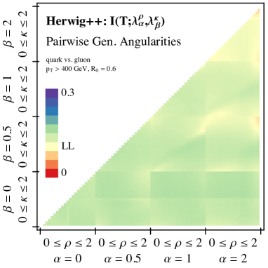
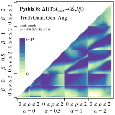
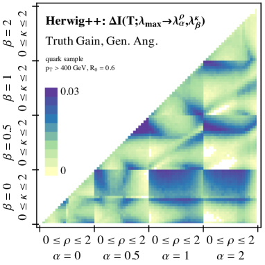
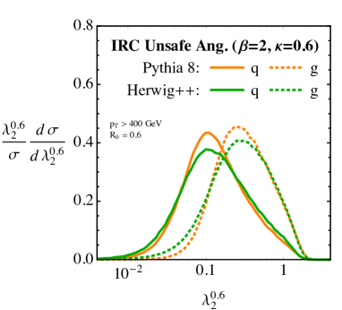
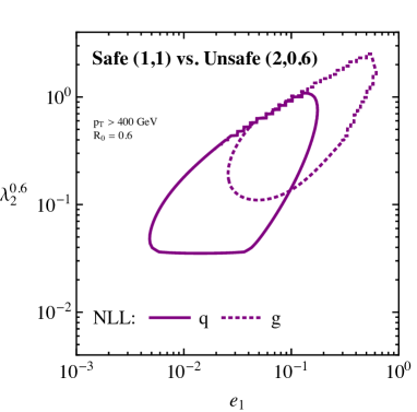
aainstitutetext: Center for Theoretical Physics, Massachusetts Institute of Technology, Cambridge, MA 02139, USAbbinstitutetext: Nikhef, Theory Group, Science Park 105, 1098 XG, Amsterdam, The Netherlandsccinstitutetext: ITFA, University of Amsterdam, Science Park 904, 1018 XE, Amsterdam, The Netherlands

Gaining (Mutual) Information about
Quark/Gluon Discrimination

Andrew J. Larkoski a    Jesse Thaler b,c    and Wouter J. Waalewijn larkoski@mit.edu jthaler@mit.edu wouterw@nikhef.nl
Abstract

Discriminating quark jets from gluon jets is an important but challenging problem in jet substructure. In this paper, we use the concept of mutual information to illuminate the physics of quark/gluon tagging. Ideal quark/gluon separation requires only one bit of truth information, so even if two discriminant variables are largely uncorrelated, they can still share the same “truth overlap”. Mutual information can be used to diagnose such situations, and thus determine which discriminant variables are redundant and which can be combined to improve performance. Using both parton showers and analytic resummation, we study a two-parameter family of generalized angularities, which includes familiar infrared and collinear (IRC) safe observables like thrust and broadening, as well as IRC unsafe variants like pTDsuperscriptsubscript𝑝𝑇𝐷p_{T}^{D} and hadron multiplicity. At leading-logarithmic (LL) order, the bulk of these variables exhibit Casimir scaling, such that their truth overlap is a universal function of the color factor ratio CA/CFsubscript𝐶𝐴subscript𝐶𝐹C_{A}/C_{F}. Only at next-to-leading-logarithmic (NLL) order can one see a difference in quark/gluon performance. For the IRC safe angularities, we show that the quark/gluon performance can be improved by combining angularities with complementary angular exponents. Interestingly, LL order, NLL order, Pythia 8, and Herwig++ all exhibit similar correlations between observables, but there are significant differences in the predicted quark/gluon discrimination power. For the IRC unsafe angularities, we show that the mutual information can be calculated analytically with the help of a nonperturbative “weighted-energy function”, providing evidence for the complementarity of safe and unsafe observables for quark/gluon discrimination.

preprint: MIT–CTP 4572 NIKHEF 2014-026

1 Introduction

Jets are collimated sprays of hadrons that act as proxies for short-distance quarks and gluons. Because quarks and gluons have different color charges, they have different showering and fragmentation patterns, and one can exploit this information to discriminate quark-initiated jets from gluon-initiated jets on a statistical basis. Quark/gluon discrimination is one of the key goals of the jet substructure community Abdesselam:2010pt ; Altheimer:2012mn ; Altheimer:2013yza . A number of quark/gluon tagging methods have been pursued Gallicchio:2011xq ; Gallicchio:2012ez ; Krohn:2012fg ; Chatrchyan:2012sn ; Pandolfi:1480598 ; Larkoski:2013eya , with corresponding performance studies CMS-PAS-JME-13-002 ; CMS-PAS-JME-13-005 ; Aad:2014gea at the Large Hadron Collider (LHC).

Two seemingly conflicting themes have emerged from these quark/gluon discrimination studies (as well as from other tagging studies). An optimistic theme is that tagging performance can be substantially improved by combining multiple jet substructure observables, as advocated in Refs. Gallicchio:2011xq ; Gallicchio:2012ez . A more pessimistic theme is that even if two discriminant variables are largely uncorrelated, their joint performance may not be much better than their individual performance. These dueling themes can be seen by comparing the results of recent tagging studies of boosted W𝑊W bosons TheATLAScollaboration:2013tia ; CMS-PAS-JME-13-006 . Since quark/gluon discrimination has so many potential physics applications, it is essential to understand why both of these themes can be true.

To achieve this goal, we pursue a twofold approach in this paper. First, we use the concept of “mutual information” to illuminate the statistical aspects of quark/gluon tagging. Mutual information characterizes the correlations between variables by counting the number of shared bits of information.111 To our knowledge, the only use of mutual information in the particle physics literature is Ref. Carruthers:1989gu , though it has been discussed recently in Ref. Narsky:2014fya as a robust measure of correlations. Elsewhere in high energy physics, mutual information is used in the study of (holographic) entanglement entropy (see e.g. Casini:2004bw ; 2008PhRvL.100g0502W ; 2009JPhA…42X4005C ; Headrick:2010zt ). Ideal quark/gluon tagging requires just one bit of “truth” information (e.g. 0=0absent0= quark and 1=1absent1= gluon), so even if a variable has many bits of total information, those bits may or may not have much overlap with the truth. For an observable a𝑎a and an equal admixture of quarks and gluons, the mutual information with the truth is

I(T;A)=da(pq(a)2log2pq(a)ptot(a)+pg(a)2log2pg(a)ptot(a)),𝐼𝑇𝐴differential-d𝑎subscript𝑝𝑞𝑎2subscript2subscript𝑝𝑞𝑎subscript𝑝tot𝑎subscript𝑝𝑔𝑎2subscript2subscript𝑝𝑔𝑎subscript𝑝tot𝑎I(T;A)=\int\mathrm{d}a\left(\frac{p_{q}(a)}{2}\log_{2}\frac{p_{q}(a)}{p_{\rm tot}(a)}+\frac{p_{g}(a)}{2}\log_{2}\frac{p_{g}(a)}{p_{\rm tot}(a)}\right), (1)

where pqsubscript𝑝𝑞p_{q} (pgsubscript𝑝𝑔p_{g}) is the probability distribution for quarks (gluons), and ptot=(pq+pg)/2subscript𝑝totsubscript𝑝𝑞subscript𝑝𝑔2p_{\rm tot}=(p_{q}+p_{g})/2. Since 0I(T;A)10𝐼𝑇𝐴10\leq I(T;A)\leq 1, we will sometimes refer to it as the “truth overlap”. In essence, the conflicting themes above can be traced to the difference between the total information (measured by e.g. the Shannon entropy) and relevant information for quark/gluon discrimination (measured by I(T;A)𝐼𝑇𝐴I(T;A)).

Refer to caption
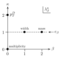
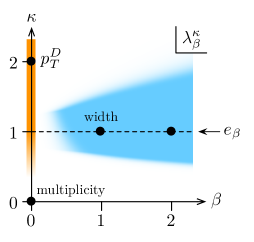
Figure 1: Visualization of the space of observables λβκsubscriptsuperscript𝜆𝜅𝛽{\lambda^{\kappa}_{\beta}}, which includes several well-known jet observables used in quark/gluon discrimination: the line κ=1𝜅1\kappa=1 corresponds to the IRC safe angularities eβsubscript𝑒𝛽{e_{\beta}}, the origin (β,κ)=(0,0)𝛽𝜅00(\beta,\kappa)=(0,0) to multiplicity, and (0,2) to pTDsuperscriptsubscript𝑝𝑇𝐷p_{T}^{D}. Here, “width” at (1,1) refers also to broadening and girth, and “mass” at (2,1) refers to jet-mass-squared divided by energy (i.e. thrust).

Second, we will introduce a two-parameter family of discriminant variables to illuminate the physics aspects of quark/gluon tagging. We will call them “generalized angularities”, which depend not only on an angular exponent β0𝛽0\beta\geq 0, but also on an energy weighting factor κ0𝜅0\kappa\geq 0. They are defined as

λβκ=ijetziκ(RiR0)β,subscriptsuperscript𝜆𝜅𝛽subscript𝑖jetsuperscriptsubscript𝑧𝑖𝜅superscriptsubscript𝑅𝑖subscript𝑅0𝛽{\lambda^{\kappa}_{\beta}}=\sum_{i\in\text{jet}}z_{i}^{\kappa}\left(\frac{R_{i}}{R_{0}}\right)^{\beta}, (2)

where zisubscript𝑧𝑖z_{i} is the momentum fraction of particle i𝑖i, Risubscript𝑅𝑖R_{i} is its rapidity/azimuth angle to a suitable axis,222To have recoil-free observables, we use the winner-take-all axis Bertolini:2013iqa ; Larkoski:2014uqa ; Salambroadening . The winner-take-all axis always coincides with one of the particles in the jet, so there is guaranteed to be at least one particle with Ri=0subscript𝑅𝑖0R_{i}=0. For β=0𝛽0\beta=0, we define λ0κ=iziκsubscriptsuperscript𝜆𝜅0subscript𝑖superscriptsubscript𝑧𝑖𝜅{\lambda^{\kappa}_{0}}=\sum_{i}z_{i}^{\kappa}. Though we will not discuss the issue of recoil Catani:1992jc ; Dokshitzer:1998kz ; Banfi:2004yd ; Larkoski:2013eya ; Larkoski:2014uqa ; Larkoski:2014bia in much detail, our analytic results require using recoil-free instead of recoil-sensitive angularities. and R0subscript𝑅0R_{0} is the jet radius. These variables are infrared and collinear (IRC) safe only for κ=1𝜅1\kappa=1. As shown in Fig. 1, certain values of (β,κ)𝛽𝜅(\beta,\kappa) correspond to well-known observables: (0,0)00(0,0) is particle multiplicity, (0,2)02(0,2) is pTDsuperscriptsubscript𝑝𝑇𝐷p_{T}^{D} Chatrchyan:2012sn ; Pandolfi:1480598 ; CMS-PAS-JME-13-005 , and the line (β,1)𝛽1(\beta,1) are the (recoil-free) angularities eβsubscript𝑒𝛽{e_{\beta}} Berger:2003iw ; Almeida:2008yp ; Ellis:2010rwa ; Larkoski:2014uqa , including broadening/width/girth at β=1𝛽1\beta=1 Rakow:1981qn ; Ellis:1986ig ; Catani:1992jc and thrust at β=2𝛽2\beta=2 Farhi:1977sg .333The recoil-free angularities are sometimes denoted as τ(β)superscript𝜏𝛽\tau^{(\beta)} Larkoski:2013eya . The generalized angularities also have the honorific notation of ϕβκsuperscriptsubscriptitalic-ϕ𝛽𝜅\phi_{\beta}^{\kappa}. We will present analytic calculations and parton shower simulations to understand the quark/gluon discrimination power of the λβκsubscriptsuperscript𝜆𝜅𝛽{\lambda^{\kappa}_{\beta}} variables.

Our analytic calculations build on previous work calculating the substructure of quark and gluon jets Almeida:2008yp ; Ellis:2010rwa ; Larkoski:2013eya ; Dasgupta:2013ihk ; Dasgupta:2013via ; Larkoski:2014wba and well as calculating angularities in e+esuperscript𝑒superscript𝑒e^{+}e^{-} event shapes Berger:2003iw ; Hornig:2009vb ; Larkoski:2014uqa . For the IRC safe angularities (κ=1𝜅1\kappa=1), we will be able to analytically study the correlations between two angularities eαsubscript𝑒𝛼{e_{\alpha}} and eβsubscript𝑒𝛽{e_{\beta}} up to next-to-leading logarithmic (NLL) accuracy. For the IRC unsafe angularities (κ1𝜅1\kappa\not=1), we can use the techniques developed in Refs. Krohn:2012fg ; Waalewijn:2012sv ; Chang:2013rca ; Chang:2013iba to introduce a new nonperturbative object called the “weighted-energy function”. For β=0𝛽0\beta=0, the discrimination power depends on the details of this object and only the dependence on the jet pTsubscript𝑝𝑇p_{T} and radius R0subscript𝑅0R_{0} is calculable. However, for κβ0.5greater-than-or-equivalent-to𝜅𝛽0.5\kappa\beta\gtrsim 0.5, just the first (logarithmic) moment of this function enters at NLL. As long as these moments are sufficiently small, we can predict the quark/gluon tagging performance for an individual λβκsubscriptsuperscript𝜆𝜅𝛽{\lambda^{\kappa}_{\beta}} to NLL accuracy, as well as study correlations between two IRC unsafe angularities to NLL.

Some of the results in this paper are well-known to experts, though perhaps not in the language we use here. On the statistical side, tagging performance is typically shown in terms of receiver operating characteristic (ROC) curves, which show the background mistag rate for a given signal efficiency. As discussed in App. A.1, ROC curves and mutual information are related to each other, and while ROC curves are perhaps more intuitive, mutual information has a closed form analytic definition and also has a nice visualization in terms of Venn diagrams. Furthermore, in App. A.2, we prove that if one observable has a better ROC curve than another, then it also has a larger truth overlap, showing that I(T;A)𝐼𝑇𝐴I(T;A) is a robust measure of tagging performance. On the physics side, λβκsubscriptsuperscript𝜆𝜅𝛽{\lambda^{\kappa}_{\beta}} is only a subset of the possible quark/gluon discriminants (see Ref. Gallicchio:2012ez for a catalog). Our goal is not to be exhaustive, but rather explain why different values of κ𝜅\kappa and β𝛽\beta are sensitive to different properties of quarks and gluons. To maximize quark/gluon performance when combining variables, clearly one wants to pick variables that are sensitive to different physical effects.

Before presenting our results, we wish to make some general remarks about the definition of “quark jets” and “gluon jets”. For most jet algorithms, quark and gluon jets are only well-defined at lowest order in αssubscript𝛼𝑠\alpha_{s} (see, however, Ref. Banfi:2006hf ). Defining quark and gluon jets to all orders in perturbation theory is a subtle and challenging problem, and becomes even more so when non-perturbative effects are taken into account. That said, quarks and gluons are well-defined if you are (deep) in the resummation region, i.e. in the limit of energetic, narrow, well-separated jets. In this regime quark/gluon radiation patterns are universal (including non-perturbative effects Stewart:2014nna ), although at NNLL soft interference effects start playing a role, introducing a dependence on the color structure of the whole event. For the analytic predictions in this paper, we will adopt a pragmatic definition: a quark (gluon) jet is what results from the showering of a quark (gluon) parton. This was also the strategy used in Ref. Larkoski:2013eya , and is sufficient to NLL accuracy. An alternative approach is to avoid trying to directly tag quarks and gluons, and instead use event categories as a well-defined proxy for jet flavor. For example, at the LHC, one can achieve a quark-enriched sample by looking at γ/W/Z𝛾𝑊𝑍\gamma/W/Z plus jet events and a gluon-enriched sample from dijet events, with further enrichment possible through judicious kinematic selections Gallicchio:2011xc . As long as one accounts for the corresponding dilution factor, the jet-based mutual information techniques in this paper will work equally well on event categories.

In Sec. 2, we review the definition of mutual information, and use it to emphasize why the joint tagging performance of two observables is a separate concept from the correlations between two observables. In Sec. 3, we show that for observables with “Casimir scaling” behavior, the quark/gluon truth overlap is a universal function of the color factor ratio CA/CFsubscript𝐶𝐴subscript𝐶𝐹C_{A}/C_{F}. In Sec. 4, we discuss the general features of the λβκsubscriptsuperscript𝜆𝜅𝛽{\lambda^{\kappa}_{\beta}} variables and show parton shower results for their mutual information. We then turn to analytic calculations, treating the IRC safe case of the angularities eβsubscript𝑒𝛽{e_{\beta}} in Sec. 5 and the more general IRC unsafe case of λβκsubscriptsuperscript𝜆𝜅𝛽{\lambda^{\kappa}_{\beta}} in Sec. 6. We conclude in Sec. 7.

2 Mutual Information

2.1 Definition

Mutual information is a measure of the shared information content of two observables. For continuous distributions of variables a𝑎a and b𝑏b, the mutual information is (see e.g. nielsen00 )

I(A;B)=dadbp(a,b)log2p(a,b)p(a)p(b),𝐼𝐴𝐵differential-d𝑎differential-d𝑏𝑝𝑎𝑏subscript2𝑝𝑎𝑏𝑝𝑎𝑝𝑏I(A;B)=\int\mathrm{d}a\,\mathrm{d}b\,p(a,b)\log_{2}\frac{p(a,b)}{p(a)p(b)}, (3)

where p(a,b)𝑝𝑎𝑏p(a,b) is the joint probability distribution (normalized to have unit integral), and p(a)𝑑bp(a,b)𝑝𝑎differential-d𝑏𝑝𝑎𝑏p(a)\equiv\int db\,p(a,b) and p(b)𝑑ap(a,b)𝑝𝑏differential-d𝑎𝑝𝑎𝑏p(b)\equiv\int da\,p(a,b) are the marginal probability distributions.444The typical notation in the information theory literature is lower case symbols (a𝑎a) to denote the observable and upper case symbols (A𝐴A) to indicate the set of possible values, such that aA𝑎𝐴a\in A. We will keep this notation for a generic observable, but switch to all lower case in Sec. 4 when we specialize to λβκsubscriptsuperscript𝜆𝜅𝛽{\lambda^{\kappa}_{\beta}}. Here, we are using base 2 logarithms such that I(A;B)=1𝐼𝐴𝐵1I(A;B)=1 corresponds to one binary bit of shared information.

In order to visualize mutual information, it is helpful to rewrite I(A;B)𝐼𝐴𝐵I(A;B) in terms of Shannon entropies H𝐻H:

I(A;B)=H(A)+H(B)H(A,B).𝐼𝐴𝐵𝐻𝐴𝐻𝐵𝐻𝐴𝐵I(A;B)=H(A)+H(B)-H(A,B). (4)

Strictly speaking, the entropy (unlike the mutual information) is not well-defined for continuous observables, though it can be made sensible by binning the distributions. For discrete-valued observables, we have

H(A)=aAp(a)log2p(a),H(A,B)=aAbBp(a,b)log2p(a,b),formulae-sequence𝐻𝐴subscript𝑎𝐴𝑝𝑎subscript2𝑝𝑎𝐻𝐴𝐵subscript𝑎𝐴subscript𝑏𝐵𝑝𝑎𝑏subscript2𝑝𝑎𝑏H(A)=-\sum_{a\in A}\,p(a)\log_{2}p(a),\qquad H(A,B)=-\sum_{a\in A}\sum_{b\in B}\,p(a,b)\log_{2}p(a,b), (5)

such that H𝐻H “counts” the number of bits of information carried by the corresponding variables. The entropies satisfy the same inequalities familiar from set theory555To derive these inequalities, consider any binned distributions p(a)𝑝𝑎p(a) and p(a,b)𝑝𝑎𝑏p(a,b). The relation H(A)0𝐻𝐴0H(A)\geq 0 follows from 0p(a)10𝑝𝑎10\leq p(a)\leq 1. The relation H(A,B)H(A)𝐻𝐴𝐵𝐻𝐴H(A,B)\geq H(A) can be derived by noting that p(a,b)p(a)𝑝𝑎𝑏𝑝𝑎p(a,b)\leq p(a) for any b𝑏b, and therefore H(A,B)=a,bp(a,b)log2p(a,b)a,bp(a,b)log2p(a)=ap(a)log2p(a)=H(A).𝐻𝐴𝐵subscript𝑎𝑏𝑝𝑎𝑏subscript2𝑝𝑎𝑏subscript𝑎𝑏𝑝𝑎𝑏subscript2𝑝𝑎subscript𝑎𝑝𝑎subscript2𝑝𝑎𝐻𝐴H(A,B)=-\sum_{a,b}\,p(a,b)\log_{2}p(a,b)\geq-\sum_{a,b}\,p(a,b)\log_{2}p(a)=-\sum_{a}\,p(a)\log_{2}p(a)=H(A). (6) The relation H(A)+H(B)H(A,B)𝐻𝐴𝐻𝐵𝐻𝐴𝐵H(A)+H(B)\geq H(A,B) follows from log2x(1x)/ln2subscript2𝑥1𝑥2-\log_{2}x\geq(1-x)/\ln 2, and therefore H(A)+H(B)H(A,B)=a,bp(a,b)log2p(a)p(b)p(a,b)1ln2a,bp(a,b)(1p(a)p(b)p(a,b))=0.𝐻𝐴𝐻𝐵𝐻𝐴𝐵subscript𝑎𝑏𝑝𝑎𝑏subscript2𝑝𝑎𝑝𝑏𝑝𝑎𝑏12subscript𝑎𝑏𝑝𝑎𝑏1𝑝𝑎𝑝𝑏𝑝𝑎𝑏0H(A)+H(B)-H(A,B)=-\sum_{a,b}p(a,b)\log_{2}\frac{p(a)p(b)}{p(a,b)}\geq\frac{1}{\ln 2}\sum_{a,b}p(a,b)\left(1-\frac{p(a)p(b)}{p(a,b)}\right)=0. (7)

0H(A)H(A,B)H(A)+H(B).0𝐻𝐴𝐻𝐴𝐵𝐻𝐴𝐻𝐵0\leq H(A)\leq H(A,B)\leq H(A)+H(B). (8)

Thus, mutual information falls in the range

0I(A;B)min{H(A),H(B)}.0𝐼𝐴𝐵𝐻𝐴𝐻𝐵0\leq I(A;B)\leq\min\{H(A),H(B)\}. (9)

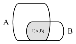
As shown in Fig. 2a, I(A;B)𝐼𝐴𝐵I(A;B) can be interpreted as the “area” of the intersection AB𝐴𝐵A\cap B in information space, and it useful for quantifying the degree of correlation between two variables, with low values corresponding less correlated variables.
Refer to caption
(a)
Refer to caption
(b)


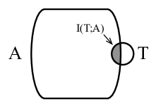
Figure 2: Left: The mutual information I(A;B)𝐼𝐴𝐵I(A;B) between observables A𝐴A and B𝐵B is visualized as the area of the shaded overlap region in information space. In keeping with the set-theoretic relation in Eq. (8), the region labelled A𝐴A has area H(A)𝐻𝐴H(A), the region labelled B𝐵B has area H(B)𝐻𝐵H(B), the union AB𝐴𝐵A\cup B has area H(A,B)𝐻𝐴𝐵H(A,B), and the intersection AB𝐴𝐵A\cap B has area I(A;B)𝐼𝐴𝐵I(A;B). Right: As a special case, we can consider the mutual information I(T;A)𝐼𝑇𝐴I(T;A) between observable A𝐴A and the truth T𝑇T (i.e. the truth overlap).

2.2 Single Variable Discrimination

For a single variable a𝑎a, we can quantify how well it performs as a signal/background discriminant by calculating how much mutual information it shares with the truth T𝑇T. Consider an event sample with signal fraction f𝑓f and background fraction (1f)1𝑓(1-f), and let t=0𝑡0t=0 for signal events and t=1𝑡1t=1 for background events. Because t𝑡t is a discrete variable, it has a well-defined Shannon entropy

H(T)=flog2f(1f)log2(1f),𝐻𝑇𝑓subscript2𝑓1𝑓subscript21𝑓H(T)=-f\log_{2}f-(1-f)\log_{2}(1-f), (10)

which is the number of available “truth bits”. The most intuitive choice is f=1/2𝑓12f=1/2 which yields H(T)=1𝐻𝑇1H(T)=1, corresponding to one bit of truth (i.e. signal =0absent0=0 vs. background =1absent1=1).

Without knowing the truth information, the measured a𝑎a distribution would be

ptot(a)=fp0(a)+(1f)p1(a),subscript𝑝tot𝑎𝑓subscript𝑝0𝑎1𝑓subscript𝑝1𝑎p_{\rm tot}(a)=f\,p_{0}(a)+(1-f)\,p_{1}(a), (11)

where p0subscript𝑝0p_{0} (p1subscript𝑝1p_{1}) is the normalized a𝑎a probability distribution for signal (background) events. With the addition of truth information, the joint probability distribution is

p(t,a)=δt0fp0(a)+δt1(1f)p1(a),𝑝𝑡𝑎subscript𝛿𝑡0𝑓subscript𝑝0𝑎subscript𝛿𝑡11𝑓subscript𝑝1𝑎p(t,a)=\delta_{t0}\,f\,p_{0}(a)+\delta_{t1}\,(1-f)\,p_{1}(a), (12)

so the mutual information between A𝐴A and the truth T𝑇T (i.e. the truth overlap) is

I(T;A)𝐼𝑇𝐴\displaystyle I(T;A) =H(T)+H(A)H(T,A)absent𝐻𝑇𝐻𝐴𝐻𝑇𝐴\displaystyle=H(T)+H(A)-H(T,A)
=da(fp0(a)log2p0(a)ptot(a)+(1f)p1(a)log2p1(a)ptot(a)).absentdifferential-d𝑎𝑓subscript𝑝0𝑎subscript2subscript𝑝0𝑎subscript𝑝tot𝑎1𝑓subscript𝑝1𝑎subscript2subscript𝑝1𝑎subscript𝑝tot𝑎\displaystyle=\int\mathrm{d}a\left(f\,p_{0}(a)\log_{2}\frac{p_{0}(a)}{p_{\rm tot}(a)}+(1-f)\,p_{1}(a)\log_{2}\frac{p_{1}(a)}{p_{\rm tot}(a)}\right). (13)

By Eq. (9) and shown in Fig. 2b,

0I(T;A)H(T).0𝐼𝑇𝐴𝐻𝑇0\leq I(T;A)\leq H(T). (14)

The mutual information I(T;A)𝐼𝑇𝐴I(T;A) quantifies how well the variable a𝑎a can separate signal and background, with I(T;A)=0𝐼𝑇𝐴0I(T;A)=0 corresponding to no discrimination power and I(T;A)=H(T)𝐼𝑇𝐴𝐻𝑇I(T;A)=H(T) corresponding to full discrimination power.

In this paper, we will focus almost exclusively on f=1/2𝑓12f=1/2 (see Eq. (1)), such that 0I(T;A)10𝐼𝑇𝐴10\leq I(T;A)\leq 1. As explained in App. A.1, by varying f𝑓f, I(T;A)𝐼𝑇𝐴I(T;A) can be related to the ROC curves typically used to quantify discrimination power. Unlike ROC curves, there is a closed-form expression for the mutual information, which makes it better suited for analytical studies. To justify that I(T;A)𝐼𝑇𝐴I(T;A) is robust measure of tagging performance, we show in App. A.2 that if one observable is Pareto optimal with respect to another (i.e. its ROC curve is everywhere improved), then the corresponding truth overlap is strictly larger. When Eq. (2.2) is applied on a sample of events generated by a Monte Carlo program, the finite sample size requires one to replace the integral by a sum over bins. Care is needed to avoid biasing the mutual information from binning, which is discussed in detail in App. A.3.

2.3 Pairwise Correlations in Discrimination

Given two variables a𝑎a and b𝑏b, I(T;A)𝐼𝑇𝐴I(T;A) and I(T;B)𝐼𝑇𝐵I(T;B) quantify how well each performs individually as signal/background discriminants. Similarly, we can assess how well a𝑎a and b𝑏b perform as joint discriminant variables by calculating

I(T;A,B)=H(T)+H(A,B)H(T,A,B).𝐼𝑇𝐴𝐵𝐻𝑇𝐻𝐴𝐵𝐻𝑇𝐴𝐵I(T;A,B)=H(T)+H(A,B)-H(T,A,B). (15)

Unlike I(A;B)𝐼𝐴𝐵I(A;B), which only tests whether or not a𝑎a and b𝑏b or correlated, I(T;A,B)𝐼𝑇𝐴𝐵I(T;A,B) tests whether the (lack of) correlations between a𝑎a and b𝑏b is useful for signal/background discrimination. Note that

max{I(T,A),I(T;B)}I(T;A,B),𝐼𝑇𝐴𝐼𝑇𝐵𝐼𝑇𝐴𝐵\max\{I(T,A),I(T;B)\}\leq I(T;A,B), (16)

such that a𝑎a and b𝑏b always have the same or better joint discrimination than either variable individually. If I(T;A,B)=max{I(T,A),I(T;B)}𝐼𝑇𝐴𝐵𝐼𝑇𝐴𝐼𝑇𝐵I(T;A,B)=\max\{I(T,A),I(T;B)\}, then there is no gain in quark/gluon discrimination in considering both a𝑎a and b𝑏b, and one of the two variables is redundant, at least for this purpose.

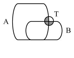
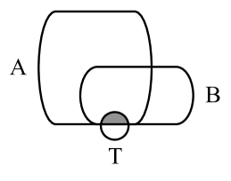
To highlight the difference between I(A;B)𝐼𝐴𝐵I(A;B) and I(T;A,B)𝐼𝑇𝐴𝐵I(T;A,B), consider Fig. 3 which shows two variables with a low degree of correlation (i.e. I(A;B)𝐼𝐴𝐵I(A;B) is relatively small). In the left example, a𝑎a and b𝑏b are both decent discriminant variables individually (i.e. A𝐴A and B𝐵B both have overlap with the truth T𝑇T), but they have considerably improved joint discrimination power (i.e. I(T;A,B)𝐼𝑇𝐴𝐵I(T;A,B) is larger than both I(T;A)𝐼𝑇𝐴I(T;A) and I(T;B)𝐼𝑇𝐵I(T;B)). In the right example, despite the fact that a𝑎a and b𝑏b are largely uncorrelated (as measured by I(A;B)𝐼𝐴𝐵I(A;B)), there is no gain in discrimination power by considering a𝑎a and b𝑏b jointly (i.e. I(T;A,B)=I(T;A)=I(T;B)𝐼𝑇𝐴𝐵𝐼𝑇𝐴𝐼𝑇𝐵I(T;A,B)=I(T;A)=I(T;B).)

In the jet substructure literature, there are known examples of both situations in Fig. 3. The left example is the ideal case (see e.g. TheATLAScollaboration:2013tia ), where two variables a𝑎a and b𝑏b give complementary information for discrimination. The right example is the more puzzling case (see e.g. CMS-PAS-JME-13-006 ), where two variables exhibit comparable discrimination power, a low degree of correlation, yet little gain in performance when considered jointly. Using mutual information, it is straightforward to diagnose and visualize this situation, helping to identify redundant variables. (Of course, redundant but largely uncorrelated variables can still be helpful for other purposes, such as calibration.)
Refer to caption
(a)
Refer to caption
(b)


Figure 3: The mutual information I(T;A,B)𝐼𝑇𝐴𝐵I(T;A,B) between observables A𝐴A, B𝐵B, and the truth T𝑇T are shown as the area of their respective intersection. Though the mutual information between A𝐴A and B𝐵B (i.e. their correlation) is the same for both figures, their overlap with the truth differs. In the left figure, the mutual information with the truth (shaded) is complementary, such that combining A𝐴A and B𝐵B increases the truth overlap. This is not so in the right figure.

3 Quark/Gluon Discrimination from Casimir Scaling

As a simple example of using mutual information, consider an observable a𝑎a that satisfies the property of “Casimir scaling”. For such an observable, the normalized cumulative distribution for quarks (ΣqsubscriptΣ𝑞\Sigma_{q}) and gluons (ΣgsubscriptΣ𝑔\Sigma_{g}) can be written as

Σq(a)=eCFr(a),Σg(a)=eCAr(a),formulae-sequencesubscriptΣ𝑞𝑎superscript𝑒subscript𝐶𝐹𝑟𝑎subscriptΣ𝑔𝑎superscript𝑒subscript𝐶𝐴𝑟𝑎\Sigma_{q}(a)=e^{-C_{F}\,r(a)},\qquad\Sigma_{g}(a)=e^{-C_{A}\,r(a)}, (17)

where r(a)𝑟𝑎r(a) is any monotonically decreasing function of a𝑎a, CF=4/3subscript𝐶𝐹43C_{F}=4/3 is the color factor for quarks, and CA=3subscript𝐶𝐴3C_{A}=3 is the color factor for gluons. As we will see in Sec. 5, the angularities eβsubscript𝑒𝛽{e_{\beta}} obey Casimir scaling at leading-logarithmic (LL) order. In Sec. 6.2, we will even find that the generalized angularities λβκsubscriptsuperscript𝜆𝜅𝛽{\lambda^{\kappa}_{\beta}} with κβ0.5greater-than-or-equivalent-to𝜅𝛽0.5\kappa\beta\gtrsim 0.5 obey Casimir scaling at LL as well.

As discussed in Ref. Larkoski:2013eya , any observable that exhibits Casimir scaling has a ROC curve of

ROC=xCA/CF=x9/4,ROCsuperscript𝑥subscript𝐶𝐴subscript𝐶𝐹superscript𝑥94\text{ROC}=x^{C_{A}/C_{F}}=x^{9/4}, (18)

where x𝑥x is the quark jet efficiency and xCA/CFsuperscript𝑥subscript𝐶𝐴subscript𝐶𝐹x^{C_{A}/C_{F}} is the gluon jet mistag rate. This result follows from making a cut a<acut𝑎subscript𝑎cuta<a_{\rm cut}, which keeps a fraction Σq(acut)subscriptΣ𝑞subscript𝑎cut\Sigma_{q}(a_{\rm cut}) of quarks and a fraction Σg(acut)=(Σq(acut))CA/CFsubscriptΣ𝑔subscript𝑎cutsuperscriptsubscriptΣ𝑞subscript𝑎cutsubscript𝐶𝐴subscript𝐶𝐹\Sigma_{g}(a_{\rm cut})=(\Sigma_{q}(a_{\rm cut}))^{C_{A}/C_{F}} of gluons. Since (approximate) Casimir scaling is so ubiquitous among quark/gluon discriminants, this explains why so many discriminant variables have such similar performance. To improve performance, one has to probe the jet beyond just its overall color charge Cisubscript𝐶𝑖C_{i}.

We can understand this same feature from the point of view of mutual information by showing that the truth overlap I(T;A)𝐼𝑇𝐴I(T;A) is a universal function of CA/CFsubscript𝐶𝐴subscript𝐶𝐹C_{A}/C_{F} for observables that exhibit Casimir scaling.666This result can also be derived from the relationship between the ROC curve and mutual information presented in App. A.1. The probability distribution for a𝑎a is just the derivative of the cumulative distribution with respect to a𝑎a:

pq(a)subscript𝑝𝑞𝑎\displaystyle p_{q}(a) =ddaΣq(a)=CFr(a)eCFr(a),absentdd𝑎subscriptΣ𝑞𝑎subscript𝐶𝐹superscript𝑟𝑎superscript𝑒subscript𝐶𝐹𝑟𝑎\displaystyle=\frac{\mathrm{d}}{\mathrm{d}a}\,\Sigma_{q}(a)=-C_{F}\,r^{\prime}(a)\,e^{-C_{F}r(a)}, (19)
pg(a)subscript𝑝𝑔𝑎\displaystyle p_{g}(a) =ddaΣg(a)=CAr(a)eCAr(a),absentdd𝑎subscriptΣ𝑔𝑎subscript𝐶𝐴superscript𝑟𝑎superscript𝑒subscript𝐶𝐴𝑟𝑎\displaystyle=\frac{\mathrm{d}}{\mathrm{d}a}\,\Sigma_{g}(a)=-C_{A}\,r^{\prime}(a)\,e^{-C_{A}r(a)}, (20)

If f𝑓f is the fraction of quark jets in the sample and (1f)1𝑓(1-f) is the fraction of gluon jets, the total probability distribution is

ptot(a)=fpq(a)+(1f)pg(a),subscript𝑝tot𝑎𝑓subscript𝑝𝑞𝑎1𝑓subscript𝑝𝑔𝑎p_{\rm tot}(a)=f\,p_{q}(a)+(1-f)\,p_{g}(a), (21)

and the truth overlap is

I(T;A)𝐼𝑇𝐴\displaystyle I(T;A) =fdapq(a)log2pq(a)ptot(a)+(1f)dapg(a)log2pg(a)ptot(a)absent𝑓differential-d𝑎subscript𝑝𝑞𝑎subscript2subscript𝑝𝑞𝑎subscript𝑝tot𝑎1𝑓differential-d𝑎subscript𝑝𝑔𝑎subscript2subscript𝑝𝑔𝑎subscript𝑝tot𝑎\displaystyle=f\int\!\mathrm{d}a\,p_{q}(a)\log_{2}\frac{p_{q}(a)}{p_{\rm tot}(a)}+(1-f)\int\!\mathrm{d}a\,p_{g}(a)\log_{2}\frac{p_{g}(a)}{p_{\rm tot}(a)}
=fda(CFr(a)eCFr(a))log2(f+(1f)CACFe(CACF)r(a))absent𝑓differential-d𝑎subscript𝐶𝐹superscript𝑟𝑎superscript𝑒subscript𝐶𝐹𝑟𝑎subscript2𝑓1𝑓subscript𝐶𝐴subscript𝐶𝐹superscript𝑒subscript𝐶𝐴subscript𝐶𝐹𝑟𝑎\displaystyle=f\int\!\mathrm{d}a\,\left(C_{F}\,r^{\prime}(a)\,e^{-C_{F}r(a)}\right)\log_{2}\left(f+(1-f)\frac{C_{A}}{C_{F}}e^{-(C_{A}-C_{F})r(a)}\right)
+(1f)da(CAr(a)eCAr(a))log2(fCFCAe(CFCA)r(a)+(1f)).1𝑓differential-d𝑎subscript𝐶𝐴superscript𝑟𝑎superscript𝑒subscript𝐶𝐴𝑟𝑎subscript2𝑓subscript𝐶𝐹subscript𝐶𝐴superscript𝑒subscript𝐶𝐹subscript𝐶𝐴𝑟𝑎1𝑓\displaystyle\quad+(1-f)\int\mathrm{d}a\,\left(C_{A}\,r^{\prime}(a)\,e^{-C_{A}r(a)}\right)\log_{2}\left(f\frac{C_{F}}{C_{A}}e^{-(C_{F}-C_{A})r(a)}+(1-f)\right). (22)

By making the change of variables

ueCFr(a),𝑢superscript𝑒subscript𝐶𝐹𝑟𝑎u\equiv e^{-C_{F}\,r(a)}, (23)

all dependence on the distribution r(a)𝑟𝑎r(a) can be removed and the integrals can be evaluated exactly. We find

I(T;A)𝐼𝑇𝐴\displaystyle I(T;A) =1ln2[f(CACF)2CFCA(1F12(1,CFCACF;CACACF;(f1)CAfCF))\displaystyle=\frac{1}{\ln 2}\bigg{[}f\frac{\left(C_{A}-C_{F}\right)^{2}}{C_{F}C_{A}}\bigg{(}1-{}_{2}F_{1}\Big{(}1,\frac{C_{F}}{C_{A}-C_{F}};\frac{C_{A}}{C_{A}-C_{F}};\frac{(f-1)C_{A}}{fC_{F}}\Big{)}\bigg{)}
fln(CACFfCACFCF)(1f)ln(1fCACFCA)],\displaystyle\qquad\qquad-f\ln\Big{(}\frac{C_{A}}{C_{F}}-f\frac{C_{A}-C_{F}}{C_{F}}\Big{)}-(1-f)\ln\Big{(}1-f\frac{C_{A}-C_{F}}{C_{A}}\Big{)}\bigg{]}, (24)

where F12(a,b;c;z)subscriptsubscript𝐹12𝑎𝑏𝑐𝑧{}_{2}F_{1}(a,b;c;z) is the hypergeometric function and ln\ln is the natural logarithm. As advertised, for any observable exhibiting Casimir scaling, I(T;A)𝐼𝑇𝐴I(T;A) is a universal function of CA/CFsubscript𝐶𝐴subscript𝐶𝐹C_{A}/C_{F}.

Setting the quark fraction f𝑓f equal to 1/2121/2 and CA/CF=9/4subscript𝐶𝐴subscript𝐶𝐹94C_{A}/C_{F}=9/4 for QCD, the mutual information for quark/gluon discrimination is

I(T;A)f=1/20.103.similar-to-or-equals𝐼subscript𝑇𝐴𝑓120.103I(T;A)_{f=1/2}\simeq 0.103. (25)

This will be the baseline value to which all observables will be compared. Note that I(T,A)𝐼𝑇𝐴I(T,A) is quite far from 111 (i.e. a full truth bit), demonstrating the inherent challenge of quark/gluon tagging.

4 Generalized Angularities

Our analytic studies of quark/gluon separation will focus on the generalized angularities λβκsubscriptsuperscript𝜆𝜅𝛽{\lambda^{\kappa}_{\beta}} defined in Eq. (2), repeated for convenience:

λβκ=ijetziκθiβ.subscriptsuperscript𝜆𝜅𝛽subscript𝑖jetsuperscriptsubscript𝑧𝑖𝜅superscriptsubscript𝜃𝑖𝛽{\lambda^{\kappa}_{\beta}}=\sum_{i\in\text{jet}}z_{i}^{\kappa}\theta_{i}^{\beta}\,. (26)

Here zisubscript𝑧𝑖z_{i} is the energy fraction and θi=Ri/R0subscript𝜃𝑖subscript𝑅𝑖subscript𝑅0\theta_{i}=R_{i}/R_{0} the angular fraction with respect to the jet radius R0subscript𝑅0R_{0}, such that 0zi,θi1formulae-sequence0subscript𝑧𝑖subscript𝜃𝑖10\leq z_{i},\theta_{i}\leq 1. We measure the angles Risubscript𝑅𝑖R_{i} with respect to the recoil-free winner-take-all axis Bertolini:2013iqa ; Larkoski:2014uqa ; Salambroadening and we use a jet algorithm that centers the jet on the winner-take-all axis, such that θi1subscript𝜃𝑖1\theta_{i}\leq 1 is strictly enforced. For the IRC safe angularities eβsubscript𝑒𝛽{e_{\beta}}, it is known that a recoil-free axis improves quark/gluon discrimination power Larkoski:2013eya . For the generalized angularities λβκsubscriptsuperscript𝜆𝜅𝛽{\lambda^{\kappa}_{\beta}}, a recoil-free axis is crucial for the calculations with βκless-than-or-similar-to𝛽𝜅\beta\lesssim\kappa, since it ensures that λβκsubscriptsuperscript𝜆𝜅𝛽{\lambda^{\kappa}_{\beta}} measures the radiation pattern around the initiating hard quark or gluon and not the displacement (i.e. recoil) of the hard parton away from the jet axis.

These variables are effective quark/gluon discriminants because they probe the angular and energetic structure of jets, both of which are sensitive to the differing color factors between quarks and gluons, among other effects. Large β𝛽\beta emphasizes wide-angle radiation whereas small β𝛽\beta emphasizes collinear radiation. Large κ𝜅\kappa emphasizes harder hadrons, whereas small κ𝜅\kappa emphasizes softer hadrons. For reference, we highlight the κ=1𝜅1\kappa=1 and β=0𝛽0\beta=0 cases:

eβλβ1subscript𝑒𝛽subscriptsuperscript𝜆1𝛽\displaystyle{e_{\beta}}\equiv{\lambda^{1}_{\beta}} =ijetziθiβ,absentsubscript𝑖jetsubscript𝑧𝑖superscriptsubscript𝜃𝑖𝛽\displaystyle=\sum_{i\in\text{jet}}z_{i}\theta_{i}^{\beta}, (27)
λ0κsubscriptsuperscript𝜆𝜅0\displaystyle{\lambda^{\kappa}_{0}} =ijetziκ.absentsubscript𝑖jetsuperscriptsubscript𝑧𝑖𝜅\displaystyle=\sum_{i\in\text{jet}}z_{i}^{\kappa}. (28)

While λ01=1subscriptsuperscript𝜆101{\lambda^{1}_{0}}=1 is a trivial observable, we can expand around κ=1𝜅1\kappa=1 to find

limκ1λ0κ=1+ijet(κ1)zilnzi,subscript𝜅1subscriptsuperscript𝜆𝜅01subscript𝑖jet𝜅1subscript𝑧𝑖subscript𝑧𝑖\lim_{\kappa\to 1}{\lambda^{\kappa}_{0}}=1+\sum_{i\in\text{jet}}(\kappa-1)z_{i}\ln z_{i}, (29)

so when we present studies for λ01subscriptsuperscript𝜆10{\lambda^{1}_{0}}, we really mean limκ1λ0κsubscript𝜅1subscriptsuperscript𝜆𝜅0\lim_{\kappa\to 1}{\lambda^{\kappa}_{0}}, which is effectively the same as the observable ijetzilnzisubscript𝑖jetsubscript𝑧𝑖subscript𝑧𝑖\sum_{i\in\text{jet}}z_{i}\ln z_{i}.

Refer to caption
(a)
Refer to caption
(b)
Refer to caption
(c)
Refer to caption
(d)
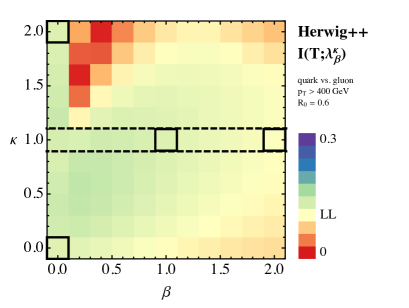
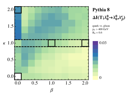
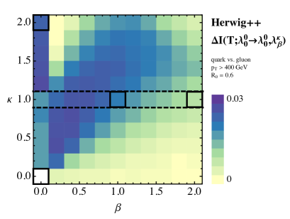
Figure 4: Parton shower study of quark/gluon discrimination for Pythia 8 (left) and Herwig++ (right). Top: quark/gluon discrimination power of λβκsubscriptsuperscript𝜆𝜅𝛽{\lambda^{\kappa}_{\beta}} as characterized by the truth overlap I(T;λβκ)𝐼𝑇subscriptsuperscript𝜆𝜅𝛽I(T;{\lambda^{\kappa}_{\beta}}). Bottom: improvement in discrimination power from supplementing multiplicity with λβκsubscriptsuperscript𝜆𝜅𝛽{\lambda^{\kappa}_{\beta}}, ΔI(T;λ00λ00,λβκ)I(T;λ00,λβκ)I(T;λ00)\Delta I(T;{\lambda^{0}_{0}}\to{\lambda^{0}_{0}},{\lambda^{\kappa}_{\beta}})\equiv I(T;{\lambda^{0}_{0}},{\lambda^{\kappa}_{\beta}})-I(T;{\lambda^{0}_{0}}). The small solid boxes correspond to the dots indicated in Fig. 1, the wide dashed box indicates the IRC safe angularities eβsubscript𝑒𝛽e_{\beta}, and “LL” in light yellow indicates the result from Casimir scaling (i.e. I(T;λβκ)0.1similar-to-or-equals𝐼𝑇subscriptsuperscript𝜆𝜅𝛽0.1I(T;{\lambda^{\kappa}_{\beta}})\simeq 0.1 from Eq. (25)).

To get a feel for the performance of the various λβκsubscriptsuperscript𝜆𝜅𝛽{\lambda^{\kappa}_{\beta}}, we can use parton shower simulations to estimate their quark/gluon truth overlap. We generate an equal admixture of quark and gluon jets (i.e. f=1/2𝑓12f=1/2) from the processes qqqq𝑞𝑞𝑞𝑞qq\to qq and gggg𝑔𝑔𝑔𝑔gg\to gg using Pythia 8.183 Sjostrand:2006za ; Sjostrand:2007gs and Herwig++ 2.6.3 Bahr:2008pv ; Gieseke:2011na at the 8 TeV LHC.777The choice of 8 TeV allows us to use the same event sample and event selection as Ref. Larkoski:2013eya . Results at 14 TeV are qualitatively similar. The transverse momenta of the jets is required to be pT>400subscript𝑝𝑇400p_{T}>400 GeV with a jet radius of R0=0.6subscript𝑅00.6R_{0}=0.6. To avoid any effects from recoil Catani:1992jc ; Dokshitzer:1998kz ; Banfi:2004yd ; Larkoski:2013eya ; Larkoski:2014bia , we identify jets using 1-jettiness Stewart:2010tn ; Thaler:2010tr as a jet finder Thaler:2011gf , taking the winner-take-all axis Bertolini:2013iqa ; Larkoski:2014uqa ; Salambroadening as the jet center. This style of jet finding always returns one perfectly circular jet cone, and FastJet 3.0.3 Cacciari:2011ma code is available from the Nsubjettiness package through the FastJet contrib project (http://fastjet.hepforge.org/contrib/).888We thank T.J. Wilkason for providing a beta version of his code.

In Figs. 4a and 4b, we show the truth overlap I(T;λβκ)𝐼𝑇subscriptsuperscript𝜆𝜅𝛽I(T;{\lambda^{\kappa}_{\beta}}) from Eq. (2.2) for different choices of λβκsubscriptsuperscript𝜆𝜅𝛽{\lambda^{\kappa}_{\beta}}.999As discussed in App. A.3, there is an important subtlety in calculating mutual information for binned samples with finite statistics. To avoid sample size artifacts, we use the same number of events to estimate pq(a)subscript𝑝𝑞𝑎p_{q}(a), pg(a)subscript𝑝𝑔𝑎p_{g}(a), and ptot(a)subscript𝑝tot𝑎p_{\rm tot}(a). Confirming the results of Refs. Gallicchio:2011xq ; Gallicchio:2012ez , one of the best single discriminant variables is λ00subscriptsuperscript𝜆00{\lambda^{0}_{0}} (i.e. hadron multiplicity). In Figs. 4c and 4d, we show the truth gain

ΔI(T;λ00λ00,λβκ)I(T;λ00,λβκ)I(T;λ00),\Delta I(T;{\lambda^{0}_{0}}\to{\lambda^{0}_{0}},{\lambda^{\kappa}_{\beta}})\equiv I(T;{\lambda^{0}_{0}},{\lambda^{\kappa}_{\beta}})-I(T;{\lambda^{0}_{0}}), (30)

which is a measure of the information gain by using a second λβκsubscriptsuperscript𝜆𝜅𝛽{\lambda^{\kappa}_{\beta}} in addition to λ00subscriptsuperscript𝜆00{\lambda^{0}_{0}}. We see that observables like λ11e1subscriptsuperscript𝜆11subscript𝑒1{\lambda^{1}_{1}}\equiv{e_{1}} (i.e. width) and λ02subscriptsuperscript𝜆20{\lambda^{2}_{0}} (i.e. pTDsuperscriptsubscript𝑝𝑇𝐷p_{T}^{D}) do add additional information, in agreement with LHC performance studies CMS-PAS-JME-13-002 ; CMS-PAS-JME-13-005 ; Aad:2014gea .

Of course, these parton shower results should be taken as just illustrative, especially since it is known that Pythia 8 typically overestimates the quark/gluon separation power Aad:2014gea . The differences between Pythia 8 and Herwig++ are quite striking, but the origin of the disagreement is not known at present. For this reason, we want to calculate I(T;λβκ)𝐼𝑇subscriptsuperscript𝜆𝜅𝛽I(T;{\lambda^{\kappa}_{\beta}}) from first principles to predict which observable (or combination of observables) has the best discrimination power, which is the subject of the next sections.

5 IRC Safe Angularities

We start our analytic studies with the IRC safe limit κ=1𝜅1\kappa=1, corresponding to the recoil-free angularities eβλβ1subscript𝑒𝛽subscriptsuperscript𝜆1𝛽{e_{\beta}}\equiv{\lambda^{1}_{\beta}}. For all β>0𝛽0\beta>0, these are IRC safe. To the order of accuracy of our calculations, eβsubscript𝑒𝛽{e_{\beta}} are identical to the energy correlation functions C1(β)superscriptsubscript𝐶1𝛽C_{1}^{(\beta)} Larkoski:2013eya . The case β=1𝛽1\beta=1 is also known as width (or broadening or girth) and β=2𝛽2\beta=2 is known as thrust (which is related to mass-squared at a fixed jet energy).

It was observed in Ref. Larkoski:2013eya that the recoil-free angularities are good quark/gluon discriminants, with better performance at fixed β𝛽\beta than the traditional recoil-sensitive angularities (i.e. angularities measured with respect to the jet momentum axis). The discrimination power of eβsubscript𝑒𝛽{e_{\beta}} increased as the angular exponent β𝛽\beta decreases towards zero, and we will verify this behavior from the mutual information viewpoint. In addition, using the double differential cross sections from Refs. Larkoski:2013paa ; Larkoski:2014tva , we can study the correlations between different angularities eαsubscript𝑒𝛼{e_{\alpha}} and eβsubscript𝑒𝛽{e_{\beta}} to show how using additional information can improve tagging performance.

5.1 Truth Overlap for One Angularity

The properties of eβsubscript𝑒𝛽{e_{\beta}} are particularly simple at LL accuracy.101010We define logarithmic accuracy through the cumulative distribution of the observable of interest. For an observable e𝑒e, the cumulative distribution has the expansion lnΣ(e)=αsln2e+αslne+αs+𝒪(αs2).Σ𝑒subscript𝛼𝑠superscript2𝑒subscript𝛼𝑠𝑒subscript𝛼𝑠𝒪superscriptsubscript𝛼𝑠2\ln\Sigma(e)=\alpha_{s}\ln^{2}e+\alpha_{s}\ln e+\alpha_{s}+{\cal O}(\alpha_{s}^{2})\ . (31) We define “LL” as keeping the leading terms in this expansion with the scaling αsln2e1similar-tosubscript𝛼𝑠superscript2𝑒1\alpha_{s}\ln^{2}e\sim 1. The normalized cumulative distribution of the angularity eβsubscript𝑒𝛽{e_{\beta}} was computed in, e.g. Ref. Larkoski:2013eya :

Σi(eβ)=exp(αsπCiβln2eβ).subscriptΣ𝑖subscript𝑒𝛽subscript𝛼𝑠𝜋subscript𝐶𝑖𝛽superscript2subscript𝑒𝛽\Sigma_{i}({e_{\beta}})=\exp\Big{(}-\frac{\alpha_{s}}{\pi}\,\frac{C_{i}}{\beta}\,\ln^{2}{e_{\beta}}\Big{)}. (32)

Here, Cisubscript𝐶𝑖C_{i} is the color of the jet: CF=4/3subscript𝐶𝐹43C_{F}=4/3 for quarks and CA=3subscript𝐶𝐴3C_{A}=3 for gluons. This distribution satisfies the Casimir scaling property of Eq. (17), and therefore the truth overlap I(T;eβ)𝐼𝑇subscript𝑒𝛽I(T;{e_{\beta}}) is given by the formula in Eq. (24), independent of β𝛽\beta.

To determine the β𝛽\beta-dependence of I(T;eβ)𝐼𝑇subscript𝑒𝛽I(T;{e_{\beta}}), we have to go to next-to-leading logarithmic (NLL) accuracy, as in Ref. Larkoski:2013eya .111111We define “NLL” as the leading terms in the expansion of Eq. (31) with the scaling αslne1similar-tosubscript𝛼𝑠𝑒1\alpha_{s}\ln e\sim 1. We use the NLL distributions for the recoil-free angularities computed in Ref. Larkoski:2014uqa (which are identical to the NLL resummation of the energy correlation functions from Ref. Banfi:2004yd ) and compute the mutual information of the angularities with truth. For β>1𝛽1\beta>1, our NLL distributions correspond to the calculations for (recoil-sensitive) angularities performed in Ref. Ellis:2010rwa . For reference, the cumulative distributions are given in App. B.1, and we determine I(T;eβ)𝐼𝑇subscript𝑒𝛽I(T;{e_{\beta}}) through numeric integration.

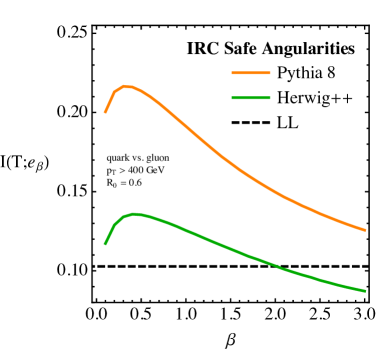
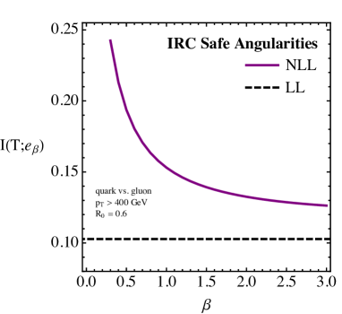
The truth overlap I(T;eβ)𝐼𝑇subscript𝑒𝛽I(T;{e_{\beta}}) as a function of the angular exponent β𝛽\beta is shown in Fig. 5 for f=1/2𝑓12f=1/2. The left plot is from the NLL calculation and the right plot shows Pythia 8 and Herwig++, using the same event generation settings as in Sec. 4 (i.e. pT>400subscript𝑝𝑇400p_{T}>400 GeV and R0=0.6subscript𝑅00.6R_{0}=0.6). The LL result from Casimir scaling is plotted for reference. We see that I(T;eβ)𝐼𝑇subscript𝑒𝛽I(T;{e_{\beta}}) increases significantly as β𝛽\beta decreases, showing that the quark/gluon discrimination improves. As discussed in Ref. Larkoski:2013eya , the qualitative β𝛽\beta-dependence is the same at NLL compared to the two parton shower programs, but there are significant numerical differences. Part of that is because the NLL result is lacking effects like nonperturbative power corrections which modify the quark/gluon discrimination power. The large difference between Pythia 8 and Herwig++ has been seen in other contexts Aad:2014gea , and the underlying reason is as-of-yet unknown.
Refer to caption
(a)
Refer to caption
(b)


Figure 5: The quark/gluon truth overlap for an individual IRC safe angularity eβsubscript𝑒𝛽{e_{\beta}} as a function of angular exponent β𝛽\beta. The transverse momentum of the jets is pT>400subscript𝑝𝑇400p_{T}>400 GeV and the jet radius is 0.60.60.6. Left: comparing the NLL truth overlap to the baseline LL result. Right: comparing the Pythia 8 and Herwig++ samples.

5.2 Truth Overlap for Two Angularities

We now turn to a study of the quark/gluon discrimination power of two angularities. This will highlight the analytic benefits of using mutual information (instead of ROC curves) to study correlated observables. Constructing the ROC curve for more than a single observable is a formidable challenge because contours of constant signal/background significance can be non-trivial functions of the observables. Typically, the procedure for determining the discrimination power is to use a multivariate analysis (MVA) such as a boosted decision tree. In contrast, mutual information is defined by simply integrating over the joint probability distribution, so all correlations between observables are automatically taken into account.

At LL accuracy, the double differential cross section of two angularities was computed in Ref. Larkoski:2013paa . For angularities eαsubscript𝑒𝛼{e_{\alpha}} and eβsubscript𝑒𝛽{e_{\beta}} with different angular exponents α>β𝛼𝛽\alpha>\beta, the double cumulative distribution is

Σi(eα,eβ)=exp[αsπCi(ln2eββ+ln2eαeβαβ)].subscriptΣ𝑖subscript𝑒𝛼subscript𝑒𝛽subscript𝛼𝑠𝜋subscript𝐶𝑖superscript2subscript𝑒𝛽𝛽superscript2subscript𝑒𝛼subscript𝑒𝛽𝛼𝛽\Sigma_{i}({e_{\alpha}},{e_{\beta}})=\exp\left[{-\frac{\alpha_{s}}{\pi}C_{i}\left(\frac{\ln^{2}{e_{\beta}}}{\beta}+\frac{\ln^{2}\frac{{e_{\alpha}}}{{e_{\beta}}}}{\alpha-\beta}\right)}\right]. (33)

At this order, the angularities satisfy the inequalities

eβ>eα,(eα)β>(eβ)α.formulae-sequencesubscript𝑒𝛽subscript𝑒𝛼superscriptsubscript𝑒𝛼𝛽superscriptsubscript𝑒𝛽𝛼{e_{\beta}}>{e_{\alpha}},\qquad({e_{\alpha}})^{\beta}>({e_{\beta}})^{\alpha}. (34)

While the LL distribution does exhibit Casimir scaling, it does so for a multivariate exponential function, so the analysis of Sec. 3 does not apply. The double differential cross section is defined by differentiating

d2σideαdeβ=(2eαeβΣi(eα,eβ))Θ0(eα,eβ),superscriptd2subscript𝜎𝑖dsubscript𝑒𝛼dsubscript𝑒𝛽superscript2subscript𝑒𝛼subscript𝑒𝛽subscriptΣ𝑖subscript𝑒𝛼subscript𝑒𝛽subscriptΘ0subscript𝑒𝛼subscript𝑒𝛽\frac{\mathrm{d}^{2}\sigma_{i}}{\mathrm{d}{e_{\alpha}}\,\mathrm{d}{e_{\beta}}}=\left(\frac{\partial^{2}}{\partial{e_{\alpha}}\,\partial{e_{\beta}}}\,\Sigma_{i}({e_{\alpha}},{e_{\beta}})\right)\Theta_{0}({e_{\alpha}},{e_{\beta}}), (35)

with explicit expressions in App. B.2. The function Θ0subscriptΘ0\Theta_{0} enforces the phase space restrictions in Eq. (34), and has to be outside of the derivatives.

At NLL accuracy, the (conjectured) double differential cross section was determined in Ref. Larkoski:2014tva by interpolating between effective theories at the eβ=eαsubscript𝑒𝛽subscript𝑒𝛼{e_{\beta}}={e_{\alpha}} and (eα)β=(eβ)αsuperscriptsubscript𝑒𝛼𝛽superscriptsubscript𝑒𝛽𝛼({e_{\alpha}})^{\beta}=({e_{\beta}})^{\alpha} boundaries of phase space. The NLL expression is given in App. B.2 for reference, and an equivalent derivation using Soft-Collinear Effective Theory (SCET) Bauer:2000ew ; Bauer:2000yr ; Bauer:2001ct ; Bauer:2001yt is given in App. C.2.
Refer to caption
(a)
Refer to caption
(b)


Refer to caption
(c)
Refer to caption
(d)


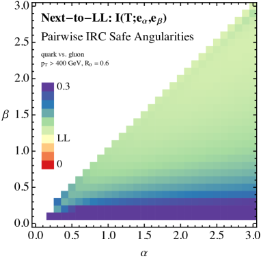
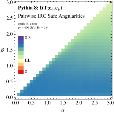
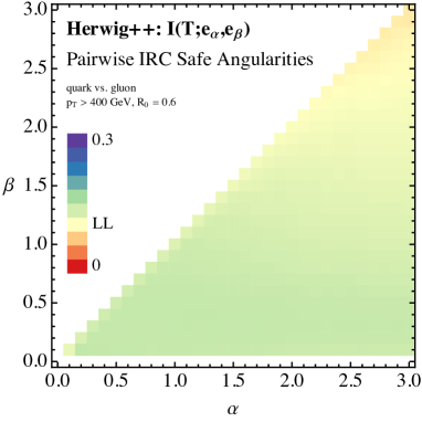
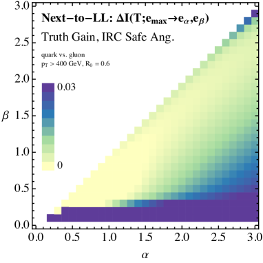
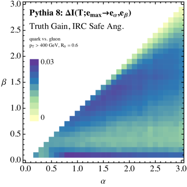
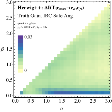
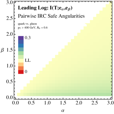
Figure 6: The quark/gluon truth overlap for pairs of IRC safe angularities (eα,eβ)subscript𝑒𝛼subscript𝑒𝛽({e_{\alpha}},{e_{\beta}}). Top: the LL and NLL analytic calculations. Bottom: the Pythia 8 and Herwig++ parton showers. The single observable LL baseline (I(T;eβ)0.1similar-to-or-equals𝐼𝑇subscript𝑒𝛽0.1I(T;{e_{\beta}})\simeq 0.1) is indicated by light yellow. Note that the LL and NLL results are only trustable for β0.5greater-than-or-equivalent-to𝛽0.5\beta\gtrsim 0.5. Also, near the α=β𝛼𝛽\alpha=\beta diagonal, the NLL results suffer from numerical issues due to the small phase space allowed by Eq. (34).

In Fig. 6 we show the truth overlap I(T;eα,eβ)𝐼𝑇subscript𝑒𝛼subscript𝑒𝛽I(T;{e_{\alpha}},{e_{\beta}}), comparing the LL expression, the NLL expression, Pythia 8, and Herwig++. As before we have set the quark fraction f=0.5𝑓0.5f=0.5, and the diagonal entries correspond to the single observable values from Fig. 5. From the baseline LL value of a single angularity in Eq. (25) (i.e. I(T;eβ)0.1similar-to-or-equals𝐼𝑇subscript𝑒𝛽0.1I(T;{e_{\beta}})\simeq 0.1) the truth overlap can be increased noticably even at LL. For example, for angularities e2subscript𝑒2e_{2} and e0.5subscript𝑒0.5e_{0.5}, the joint truth overlap is greater than 0.120.120.12 at LL. At NLL, the discrimination power uniformly rises, as expected from Fig. 5. Because our NLL expressions do not account for the nonperturbative region of phase space, one should be cautious interpreting the results for β0.5less-than-or-similar-to𝛽0.5\beta\lesssim 0.5. Turning to the parton showers, they give quite different prediction for I(T;eα,eβ)𝐼𝑇subscript𝑒𝛼subscript𝑒𝛽I(T;{e_{\alpha}},{e_{\beta}}), with Pythia 8 even more optimistic than the NLL result and Herwig++ closer to the LL result.

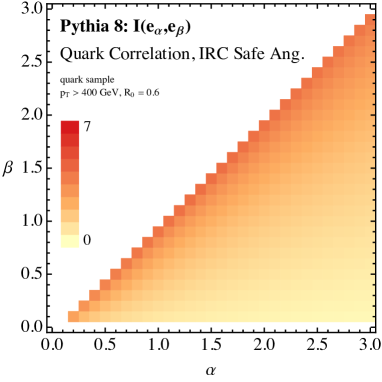
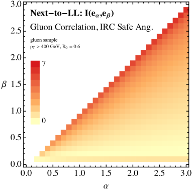
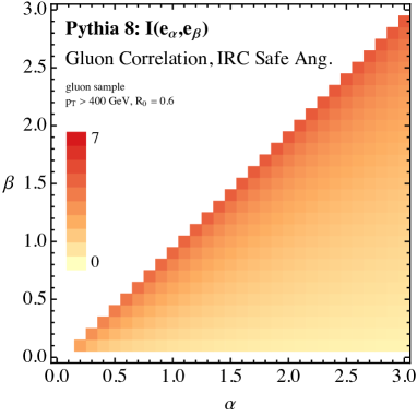
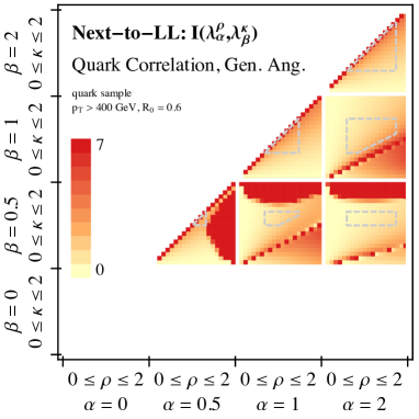
The large numerical differences between these methods highlights the considerable theoretical uncertainties present in quark/gluon discrimination. It is important to note that these large differences are not present when trying to model quarks and gluons individually, and only arise in the context of discrimination. In App. D we show the mutual information I(eα;eβ)𝐼subscript𝑒𝛼subscript𝑒𝛽I({e_{\alpha}};{e_{\beta}}), which measures the degree of correlation between two angularities on separate quark and gluon samples. The four methods (LL, NLL, Pythia 8, and Herwig++) show much closer agreement for I(eα;eβ)𝐼subscript𝑒𝛼subscript𝑒𝛽I({e_{\alpha}};{e_{\beta}}) than for I(T;eα,eβ)𝐼𝑇subscript𝑒𝛼subscript𝑒𝛽I(T;{e_{\alpha}},{e_{\beta}}), suggesting that the truth overlap is more sensitive to subtle (and difficult to predict) differences between quark and gluon jets.

For completeness, in App. D we show the truth gain

ΔI(T,emaxeα,eβ)I(T;eα,eβ)max{I(T;eα),I(T;eβ)},\Delta I(T,e_{\rm max}\to{e_{\alpha}},{e_{\beta}})\equiv I(T;{e_{\alpha}},{e_{\beta}})-\max\{I(T;{e_{\alpha}}),I(T;{e_{\beta}})\}, (36)

which makes it easier to see that there is improved quark/gluon discrimination power from measuring two angularities instead of just one.121212Of course, while mutual information is helpful to characterize the possible gains from combining observables, a multivariate analysis is still needed to realize these gains in practice. As discussed in App. B.4, it is challenging to determine the optimal cuts analytically, even at LL. Alternatively, in the spirit of Ref. Soper:2011cr , one could use the ratio of the quark/gluon double differential distributions as a weighting factor. Roughly speaking, pairs of angularities with the smallest values of I(eα;eβ)𝐼subscript𝑒𝛼subscript𝑒𝛽I({e_{\alpha}};{e_{\beta}}) (i.e. least correlation) lead to the largest increase in I(T;eα,eβ)𝐼𝑇subscript𝑒𝛼subscript𝑒𝛽I(T;{e_{\alpha}},{e_{\beta}}) (i.e. discrimination power), though there is considerable variability. Because the four methods have different predictions for which angularities should be combined, care should be taken when using any of these methods to estimate quark/gluon discrimination performance.

6 IRC Unsafe Angularities

We now turn to the more interesting case of the IRC unsafe angularities with κ1𝜅1\kappa\not=1. As seen in Sec. 4 and known in the literature, hadron multiplicity (λ00subscriptsuperscript𝜆00{\lambda^{0}_{0}}) and pTDsuperscriptsubscript𝑝𝑇𝐷p_{T}^{D} (λ02subscriptsuperscript𝜆20{\lambda^{2}_{0}}) are effective quark/gluon discriminants. But much of the rest of the (κ,β)𝜅𝛽(\kappa,\beta) plane is still unexplored (apart from the angularity line at κ=1𝜅1\kappa=1).

One challenge to gaining an analytic understanding of the κ1𝜅1\kappa\neq 1 case is that λβκsubscriptsuperscript𝜆𝜅𝛽{\lambda^{\kappa}_{\beta}} is collinear unsafe (unlike eβsubscript𝑒𝛽{e_{\beta}} studied above). This introduces an intrinsic sensitivity to nonperturbative physics that describes how the emitted radiation is split into hadrons, prohibiting a purely perturbative calculation. That said, using the techniques developed in Refs. Krohn:2012fg ; Waalewijn:2012sv ; Chang:2013rca ; Chang:2013iba , we can encode the nonperturbative information into a “weighted-energy function” which can be extracted from data. In fact, for β>0𝛽0\beta>0, we will only need a few nonperturbative parameters (and not a whole function) to characterize the distributions.
Refer to caption
Figure 7: The regions of the space of observables λβκsubscriptsuperscript𝜆𝜅𝛽{\lambda^{\kappa}_{\beta}} that we calculate are shown in orange (β=0𝛽0\beta=0 and κ0.5greater-than-or-equivalent-to𝜅0.5\kappa\gtrsim 0.5, Sec. 6.1) and blue (βκ0.5greater-than-or-equivalent-to𝛽𝜅0.5\beta\kappa\gtrsim 0.5 and βκ/(1κ)26greater-than-or-equivalent-to𝛽𝜅superscript1𝜅26\beta\kappa/(1-\kappa)^{2}\gtrsim 6, Sec. 6.2). As explained in Sec. 6.2, the funny shape of the blue region is due to a combination of perturbative and nonperturbative constraints.

Strictly speaking our calculations will only be valid for κ0.5greater-than-or-equivalent-to𝜅0.5\kappa\gtrsim 0.5. The reason is that as κ0𝜅0\kappa\to 0 the observable also becomes infrared unsafe, further complicating calculations (as discussed in the context of hadron multiplicities in e.g. Ref. Capella:1999ms ; Bolzoni:2012ii ). Also note that the β=0𝛽0\beta=0 and β>0𝛽0\beta>0 regimes are very different in how they treat collinear radiation, so we will consider them separately. The approximate range of validity of the calculations are shown in Fig. 7.

6.1 The β=0𝛽0\beta=0 Regime

We start with the β=0𝛽0\beta=0 case with λ0κsubscriptsuperscript𝜆𝜅0{\lambda^{\kappa}_{0}}. Recall from Eq. (29) that λ01subscriptsuperscript𝜆10{\lambda^{1}_{0}} effectively refers to the observable izilnzisubscript𝑖subscript𝑧𝑖subscript𝑧𝑖\sum_{i}z_{i}\ln z_{i}. In order to study these observables, we need to introduce a nonperturbative object called the weighted-energy function Fκi(x,μ)subscriptsuperscript𝐹𝑖𝜅𝑥𝜇F^{i}_{\kappa}(x,\mu) that describes how the energy of a jet is distributed among its constituent hadrons. Here, i𝑖i labels the flavor of the jet. This object is similar to the charge distribution Waalewijn:2012sv and the track function Chang:2013rca ; Chang:2013iba which describe other aspects of the fragmentation of quarks and gluons into hadrons.

The quark weighted-energy function has the following operator definition

Fκq(x,μ)subscriptsuperscript𝐹𝑞𝜅𝑥𝜇\displaystyle F^{q}_{\kappa}(x,\mu) =12NcHδ(xhH(zh)κ)absent12subscript𝑁𝑐subscript𝐻𝛿𝑥subscript𝐻superscriptsubscript𝑧𝜅\displaystyle=\frac{1}{2N_{c}}\,\sum_{H}\delta\Big{(}x-\sum_{h\in H}(z_{h})^{\kappa}\Big{)}
×tr[(γ0+γ3)0|[(2π)3δ(k+p^0+p^3)δ2(p^)ψ]|HH|ψ¯|0].absenttrdelimited-[]superscript𝛾0superscript𝛾3quantum-operator-product0delimited-[]superscript2𝜋3𝛿superscript𝑘superscript^𝑝0superscript^𝑝3superscript𝛿2subscript^𝑝perpendicular-to𝜓𝐻quantum-operator-product𝐻¯𝜓0\displaystyle\quad\times\mathrm{tr}\Big{[}(\gamma^{0}+\gamma^{3})\,\big{\langle}0\big{|}\big{[}(2\pi)^{3}\delta(k^{-}+\hat{p}^{0}+\hat{p}^{3})\delta^{2}(\hat{p}_{\perp})\psi\big{]}\big{|}H\big{\rangle}\big{\langle}H\big{|}\overline{\psi}\big{|}0\big{\rangle}\Big{]}\,. (37)

Here ψ𝜓\psi is the quark field, with momentum fixed by the δ𝛿\delta functions involving the momentum operator p^^𝑝\hat{p}, H𝐻H denotes a hadronic final state, and zh=(ph0+ph3)/ksubscript𝑧superscriptsubscript𝑝0superscriptsubscript𝑝3superscript𝑘z_{h}=(p_{h}^{0}+p_{h}^{3})/k^{-} is the momentum fraction carried by the hadron hH𝐻h\in H. (The only dependence on ksuperscript𝑘k^{-} is through zhsubscript𝑧z_{h}.) There is a similar definition for the gluon weighted-energy function, and we have suppressed eikonal Wilson lines needed for gauge invariance. These functions are normalized such that

0dxFκi(x,μ)=1.superscriptsubscript0differential-d𝑥subscriptsuperscript𝐹𝑖𝜅𝑥𝜇1\int_{0}^{\infty}\!\mathrm{d}x\,F^{i}_{\kappa}(x,\mu)=1. (38)

As a point of reference, if the hadrons were weighted by their charge, then Fκi(x)subscriptsuperscript𝐹𝑖𝜅𝑥F^{i}_{\kappa}(x) would be the jet charge function Di(x,κ,μ)subscript𝐷𝑖𝑥𝜅𝜇D_{i}(x,\kappa,\mu) Waalewijn:2012sv . Alternatively, for κ=1𝜅1\kappa=1 and restricted to charged particles, this would be the track function Ti(x,μ)subscript𝑇𝑖𝑥𝜇T_{i}(x,\mu) Chang:2013rca ; Chang:2013iba .

At LO, the cross section differential in λ0κsubscriptsuperscript𝜆𝜅0{\lambda^{\kappa}_{0}} for a parton of flavor i𝑖i is simply

1σidσidλ0κ=dxFκi(x,μ)δ(λ0κx),1subscript𝜎𝑖dsubscript𝜎𝑖dsubscriptsuperscript𝜆𝜅0differential-d𝑥subscriptsuperscript𝐹𝑖𝜅𝑥𝜇𝛿subscriptsuperscript𝜆𝜅0𝑥\frac{1}{\sigma_{i}}\frac{\mathrm{d}\sigma_{i}}{\mathrm{d}{\lambda^{\kappa}_{0}}}=\int\mathrm{d}x\,F^{i}_{\kappa}(x,\mu)\,\delta({\lambda^{\kappa}_{0}}-x), (39)

meaning that at this order, Fκi(x,μ)subscriptsuperscript𝐹𝑖𝜅𝑥𝜇F^{i}_{\kappa}(x,\mu) gives the λ0κsubscriptsuperscript𝜆𝜅0{\lambda^{\kappa}_{0}} distribution directly, with x=λ0κ𝑥subscriptsuperscript𝜆𝜅0x={\lambda^{\kappa}_{0}}. The dependence on the jet pTsubscript𝑝𝑇p_{T} and jet radius R0subscript𝑅0R_{0} enters through the scale choice μ=pTR0𝜇subscript𝑝𝑇subscript𝑅0\mu=p_{T}R_{0}. At NLO, the cross section is Waalewijn:2012sv

1σidσidλ0κ1subscript𝜎𝑖dsubscript𝜎𝑖dsubscriptsuperscript𝜆𝜅0\displaystyle\frac{1}{\sigma_{i}}\frac{\mathrm{d}\sigma_{i}}{\mathrm{d}{\lambda^{\kappa}_{0}}} =12j,kdx1dx2dz𝒥ij(pTR0,z,μ)2(2π)3Ji(pTR0,μ)absent12subscript𝑗𝑘differential-dsubscript𝑥1differential-dsubscript𝑥2differential-d𝑧subscript𝒥𝑖𝑗subscript𝑝𝑇subscript𝑅0𝑧𝜇2superscript2𝜋3subscript𝐽𝑖subscript𝑝𝑇subscript𝑅0𝜇\displaystyle=\frac{1}{2}\sum_{j,k}\int\!\mathrm{d}x_{1}\,\mathrm{d}x_{2}\,\mathrm{d}z\,\frac{{\mathcal{J}}_{ij}(p_{T}R_{0},z,\mu)}{2(2\pi)^{3}J_{i}(p_{T}R_{0},\mu)}
×Fκj(x1,μ)Fκk(x2,μ)δ(λ0κzκx1(1z)κx2).absentsubscriptsuperscript𝐹𝑗𝜅subscript𝑥1𝜇subscriptsuperscript𝐹𝑘𝜅subscript𝑥2𝜇𝛿subscriptsuperscript𝜆𝜅0superscript𝑧𝜅subscript𝑥1superscript1𝑧𝜅subscript𝑥2\displaystyle\quad\times F^{j}_{\kappa}(x_{1},\mu)F^{k}_{\kappa}(x_{2},\mu)\,\delta\big{(}{\lambda^{\kappa}_{0}}-z^{\kappa}x_{1}-(1-z)^{\kappa}x_{2}\big{)}\,. (40)

The ratio 𝒥ij/Jisubscript𝒥𝑖𝑗subscript𝐽𝑖{\mathcal{J}}_{ij}/J_{i} describes the perturbative splitting ijk𝑖𝑗𝑘i\to jk, where j𝑗j has momentum fraction z𝑧z (see also Refs. Procura:2009vm ; Jain:2011xz ). By including these NLO corrections, the perturbative uncertainty (μ𝜇\mu-dependence) is reduced.

The weighted-energy functions are purely nonperturbative, so in that sense, we are not really able to predict the quark/gluon discrimination power of the λ0κsubscriptsuperscript𝜆𝜅0{\lambda^{\kappa}_{0}} variables. But Fκi(x,μ)subscriptsuperscript𝐹𝑖𝜅𝑥𝜇F^{i}_{\kappa}(x,\mu) does have a perturbative renormalization group evolution Waalewijn:2012sv ,

μμFκi(x,μ)𝜇𝜇superscriptsubscript𝐹𝜅𝑖𝑥𝜇\displaystyle\mu\frac{\partial}{\partial\mu}\,F_{\kappa}^{i}(x,\mu) =12j,kdzdx1dx2αsπPijk(z)absent12subscript𝑗𝑘differential-d𝑧differential-dsubscript𝑥1differential-dsubscript𝑥2subscript𝛼𝑠𝜋subscript𝑃𝑖𝑗𝑘𝑧\displaystyle=\frac{1}{2}\sum_{j,k}\int\!\mathrm{d}z\,\mathrm{d}x_{1}\,\mathrm{d}x_{2}\,\frac{\alpha_{s}}{\pi}P_{i\to jk}(z)
×Fκj(x1,μ)Fκk(x2,μ)δ(x(1z)κx1zκx2).absentsuperscriptsubscript𝐹𝜅𝑗subscript𝑥1𝜇superscriptsubscript𝐹𝜅𝑘subscript𝑥2𝜇𝛿𝑥superscript1𝑧𝜅subscript𝑥1superscript𝑧𝜅subscript𝑥2\displaystyle\quad\times F_{\kappa}^{j}(x_{1},\mu)F_{\kappa}^{k}(x_{2},\mu)\,\delta\big{(}x\!-\!(1\!-\!z)^{\kappa}x_{1}\!-\!z^{\kappa}x_{2}\big{)}. (41)

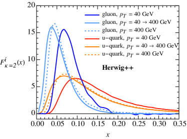
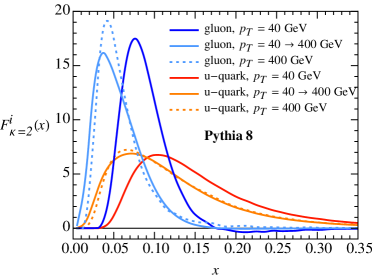
Thus, one can measure Fκi(x,μ)subscriptsuperscript𝐹𝑖𝜅𝑥𝜇F^{i}_{\kappa}(x,\mu) at one scale (ideally in pure quark/gluon samples), and then evolve to a different scale. This DGLAP Gribov:1972ri ; Georgi:1951sr ; Gross:1974cs ; Altarelli:1977zs ; Dokshitzer:1977sg evolution of Fκisubscriptsuperscript𝐹𝑖𝜅F^{i}_{\kappa} corresponds to the emissions described by a parton shower in Monte Carlo programs. We have implemented these evolution equations for pTDsuperscriptsubscript𝑝𝑇𝐷p_{T}^{D} (λ02subscriptsuperscript𝜆20{\lambda^{2}_{0}}), reproducing the dependence on the jet pTsubscript𝑝𝑇p_{T} observed in Pythia 8 and Herwig++, as shown in Fig. 8.
Refer to caption
(a)
Refer to caption
(b)


Figure 8: The weighted-energy function Fκ=2i(x)subscriptsuperscript𝐹𝑖𝜅2𝑥F^{i}_{\kappa=2}(x) for pTDsuperscriptsubscript𝑝𝑇𝐷p_{T}^{D} for u𝑢u-quarks (red) and gluons (blue), extracted from Pythia 8 (left) and Herwig++ (right). The darker solid curve is the parton shower results extracted at the scale 40 GeV, the lighter solid curve is the evolution from 40 GeV to 400 GeV using Eq. (6.1), and the dotted curve is the parton shower results at 400 GeV. In all cases, we are incorporating the NLO corrections in Eq. (6.1), which is why Fκ=2i(x)subscriptsuperscript𝐹𝑖𝜅2𝑥F^{i}_{\kappa=2}(x) can be negative.

The weighted-energy functions are sufficient for understanding a single λ0κsubscriptsuperscript𝜆𝜅0{\lambda^{\kappa}_{0}}, but if we want to study correlations between a pair of λ0ρsubscriptsuperscript𝜆𝜌0{\lambda^{\rho}_{0}} and λ0κsubscriptsuperscript𝜆𝜅0{\lambda^{\kappa}_{0}}, then we would need a double weighted-energy function:

Fρ,κi(x1,x2;μ).superscriptsubscript𝐹𝜌𝜅𝑖subscript𝑥1subscript𝑥2𝜇F_{\rho,\kappa}^{i}(x_{1},x_{2};\mu). (42)

This is defined analogously to Eq. (6.1), albeit with the double measurement

δ(x1hH(zh)ρ)δ(x2hH(zh)κ).𝛿subscript𝑥1subscript𝐻superscriptsubscript𝑧𝜌𝛿subscript𝑥2subscript𝐻superscriptsubscript𝑧𝜅\delta\Big{(}x_{1}-\sum_{h\in H}(z_{h})^{\rho}\Big{)}\,\delta\Big{(}x_{2}-\sum_{h\in H}(z_{h})^{\kappa}\Big{)}. (43)

This object also has a renormalization group evolution analogous to Eq. (6.1). In Sec. 6.3, we will use the fact that

dx1Fρ,κi(x1,x2;μ)=Fκi(x2,μ)differential-dsubscript𝑥1superscriptsubscript𝐹𝜌𝜅𝑖subscript𝑥1subscript𝑥2𝜇superscriptsubscript𝐹𝜅𝑖subscript𝑥2𝜇\int\mathrm{d}x_{1}\,F_{\rho,\kappa}^{i}(x_{1},x_{2};\mu)=F_{\kappa}^{i}(x_{2},\mu) (44)

when we study correlations between the β>0𝛽0\beta>0 angularities.

Refer to caption
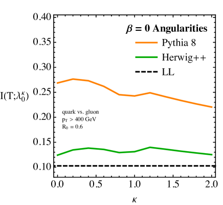
Figure 9: The quark/gluon truth overlap for an individual generalized angularity λ0κsubscriptsuperscript𝜆𝜅0{\lambda^{\kappa}_{0}} as a function of the energy-weighting power κ𝜅\kappa. Here, we are comparing the Pythia 8 and Herwig++ samples to the LL baseline.
Refer to caption
(a)
Refer to caption
(b)


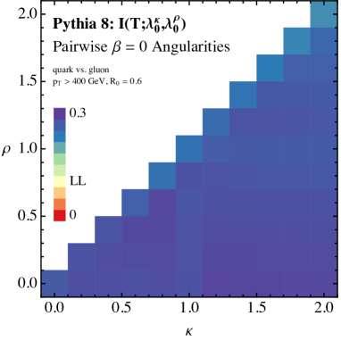
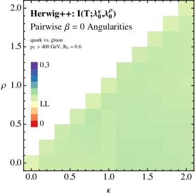
Figure 10: The quark/gluon truth overlap for pairs of β=0𝛽0\beta=0 angularities (λ0ρ,λ0κ)subscriptsuperscript𝜆𝜌0subscriptsuperscript𝜆𝜅0({\lambda^{\rho}_{0}},{\lambda^{\kappa}_{0}}), comparing the Pythia 8 and Herwig++ parton showers.

Since our analytic calculations are limited by our lack of knowledge of the nonperturbative function Fκisuperscriptsubscript𝐹𝜅𝑖F_{\kappa}^{i}, we close our discussion of β=0𝛽0\beta=0 by simply showing the quark/gluon truth overlap extracted from Pythia 8 and Herwig++. In Fig. 9, we show the truth overlap of a single λ0κsubscriptsuperscript𝜆𝜅0{\lambda^{\kappa}_{0}} and in Fig. 10 for a pair of the generalized angularities, λ0κsubscriptsuperscript𝜆𝜅0{\lambda^{\kappa}_{0}} and λ0ρsubscriptsuperscript𝜆𝜌0{\lambda^{\rho}_{0}}. Both figures are quite striking in illustrating the substantial difference in discrimination power predicted by Pythia 8 and Herwig++. Interestingly, the truth overlaps of Pythia 8 and Herwig++ seem to be related by a simple scaling of the value, with otherwise similar structures visible over the range of observables. This might point to the source of the discrepancy in the physics descriptions between Pythia 8 and Herwig++, but is beyond the scope of this paper.

6.2 The β>0𝛽0\beta>0 Regime

For β>0𝛽0\beta>0, the generalized angularities λβκsubscriptsuperscript𝜆𝜅𝛽{\lambda^{\kappa}_{\beta}} are collinear safe with respect to emissions at θ=0𝜃0\theta=0, but collinear unsafe with respect to wide-angle emissions. This is precisely the same situation as for the track thrust study in Ref. Chang:2013iba , so we can adapt those methods here. In particular, the jet can be described by a number of perturbative gluon emissions that can then be matched onto separate weighted-energy functions Fκi(x,μ)subscriptsuperscript𝐹𝑖𝜅𝑥𝜇F^{i}_{\kappa}(x,\mu). At (N)LL order, the emissions (including the weighted-energy functions) exponentiate, allowing us to predict the performance of λβκsubscriptsuperscript𝜆𝜅𝛽{\lambda^{\kappa}_{\beta}} for quark/gluon discrimination.

A jet with a single parton has λβκ=0subscriptsuperscript𝜆𝜅𝛽0{\lambda^{\kappa}_{\beta}}=0, since the reference axis will align with that parton. For two partons, the winner-take-all axis will align with the harder parton. Ignoring fixed-order corrections, we can assume that the harder parton is the initiating parton (i.e. quark for a quark jet) such that the λβκsubscriptsuperscript𝜆𝜅𝛽{\lambda^{\kappa}_{\beta}} distribution is determined by the emitted soft gluon. In the LO approximation for narrow jets, we can use splitting functions

1σidσidλβκ=01dθθ01dzαsπPiig(z)0dxFκg(x,μ)δ(λβκxzκθβ),1subscript𝜎𝑖dsubscript𝜎𝑖dsubscriptsuperscript𝜆𝜅𝛽superscriptsubscript01d𝜃𝜃superscriptsubscript01differential-d𝑧subscript𝛼𝑠𝜋subscript𝑃𝑖𝑖𝑔𝑧superscriptsubscript0differential-d𝑥subscriptsuperscript𝐹𝑔𝜅𝑥𝜇𝛿subscriptsuperscript𝜆𝜅𝛽𝑥superscript𝑧𝜅superscript𝜃𝛽\frac{1}{\sigma_{i}}\frac{\mathrm{d}\sigma_{i}}{\mathrm{d}{\lambda^{\kappa}_{\beta}}}=\int_{0}^{1}\frac{\mathrm{d}\theta}{\theta}\int_{0}^{1}\mathrm{d}z\,\frac{\alpha_{s}}{\pi}P_{i\to ig}(z)\int_{0}^{\infty}\mathrm{d}x\,F^{g}_{\kappa}(x,\mu)\,\delta({\lambda^{\kappa}_{\beta}}-xz^{\kappa}\theta^{\beta}), (45)

where Piig(z)subscript𝑃𝑖𝑖𝑔𝑧P_{i\to ig}(z) is the splitting function for parton flavor i𝑖i to emit a soft gluon with momentum fraction z𝑧z.

We can achieve (N)LL resummation by considering the strongly-ordered limit where the λβκsubscriptsuperscript𝜆𝜅𝛽{\lambda^{\kappa}_{\beta}} distribution is determined by the hardest emissions in the jet. For the strongly-ordered limit to make sense, we assume that Fκg(x,μ)subscriptsuperscript𝐹𝑔𝜅𝑥𝜇F^{g}_{\kappa}(x,\mu) is non-singular and does not have support over a hierarchically large range in x𝑥x, such that the emission with, say, the largest value of zκθβsuperscript𝑧𝜅superscript𝜃𝛽z^{\kappa}\theta^{\beta} also typically has the largest value of λβκsubscriptsuperscript𝜆𝜅𝛽{\lambda^{\kappa}_{\beta}}. This then allows us to use the logic of CAESAR Banfi:2004yd to determine the λβκsubscriptsuperscript𝜆𝜅𝛽{\lambda^{\kappa}_{\beta}} distribution up to NLL order (ignoring non-global effects Dasgupta:2001sh ).

In the CAESAR approach, the one-gluon distribution in Eq. (45) is interpreted as the radiator function:

Ri(λβκ)=01dθθ01dzαs(pTzθ)πPiig(z)0dxFκg(x,μ)Θ(xzκθβλβκ),subscript𝑅𝑖subscriptsuperscript𝜆𝜅𝛽superscriptsubscript01d𝜃𝜃superscriptsubscript01differential-d𝑧subscript𝛼𝑠subscript𝑝𝑇𝑧𝜃𝜋subscript𝑃𝑖𝑖𝑔𝑧superscriptsubscript0differential-d𝑥subscriptsuperscript𝐹𝑔𝜅𝑥𝜇Θ𝑥superscript𝑧𝜅superscript𝜃𝛽subscriptsuperscript𝜆𝜅𝛽R_{i}({\lambda^{\kappa}_{\beta}})=\int_{0}^{1}\frac{\mathrm{d}\theta}{\theta}\int_{0}^{1}\!\mathrm{d}z\,\frac{\alpha_{s}(p_{T}z\theta)}{\pi}P_{i\to ig}(z)\int_{0}^{\infty}\!\mathrm{d}x\,F^{g}_{\kappa}(x,\mu)\,\Theta(xz^{\kappa}\theta^{\beta}-{\lambda^{\kappa}_{\beta}}), (46)

where αssubscript𝛼𝑠\alpha_{s} is now a running coupling evaluated to two-loop order in the CMW scheme Catani:1990rr . This yields the cumulative distribution accurate to NLL

Σi(λβκ)=eγERi(λβκ)Γ(1+Ri(λβκ))eRi(λβκ),subscriptΣ𝑖subscriptsuperscript𝜆𝜅𝛽superscript𝑒subscript𝛾𝐸superscriptsubscript𝑅𝑖subscriptsuperscript𝜆𝜅𝛽Γ1superscriptsubscript𝑅𝑖subscriptsuperscript𝜆𝜅𝛽superscript𝑒subscript𝑅𝑖subscriptsuperscript𝜆𝜅𝛽\Sigma_{i}({\lambda^{\kappa}_{\beta}})=\frac{e^{-\gamma_{E}R_{i}^{\prime}({\lambda^{\kappa}_{\beta}})}}{\Gamma(1+R_{i}^{\prime}({\lambda^{\kappa}_{\beta}}))}e^{-R_{i}({\lambda^{\kappa}_{\beta}})}, (47)

where γEsubscript𝛾𝐸\gamma_{E} is the Euler-Mascheroni constant, ΓΓ\Gamma is the gamma function, and RidRi/dlnλβκsuperscriptsubscript𝑅𝑖dsubscript𝑅𝑖dsubscriptsuperscript𝜆𝜅𝛽R_{i}^{\prime}\equiv-\mathrm{d}R_{i}/\mathrm{d}\ln{\lambda^{\kappa}_{\beta}} is the logarithmic derivative. The cross section is obtained via

1σidσidλβκ=ddλβκΣi(λβκ).1subscript𝜎𝑖dsubscript𝜎𝑖dsubscriptsuperscript𝜆𝜅𝛽ddsubscriptsuperscript𝜆𝜅𝛽subscriptΣ𝑖subscriptsuperscript𝜆𝜅𝛽\frac{1}{\sigma_{i}}\frac{\mathrm{d}\sigma_{i}}{\mathrm{d}{\lambda^{\kappa}_{\beta}}}=\frac{\mathrm{d}}{\mathrm{d}{\lambda^{\kappa}_{\beta}}}\Sigma_{i}({\lambda^{\kappa}_{\beta}}). (48)

We can already learn a lot from Eq. (47) by considering just the LL limit. In that limit, we can drop the prefactor terms involving Rsuperscript𝑅R^{\prime}, fix the coupling αssubscript𝛼𝑠\alpha_{s}, and take Piig(z)=2Ci/zsubscript𝑃𝑖𝑖𝑔𝑧2subscript𝐶𝑖𝑧P_{i\to ig}(z)=2C_{i}/z. In that case we find

Ri(λβκ)LLαsπCiβκλβκdxFκg(x,μ)ln2λβκx.superscriptsimilar-to-or-equalsLLsubscript𝑅𝑖subscriptsuperscript𝜆𝜅𝛽subscript𝛼𝑠𝜋subscript𝐶𝑖𝛽𝜅superscriptsubscriptsubscriptsuperscript𝜆𝜅𝛽differential-d𝑥subscriptsuperscript𝐹𝑔𝜅𝑥𝜇superscript2subscriptsuperscript𝜆𝜅𝛽𝑥R_{i}({\lambda^{\kappa}_{\beta}})\stackrel{{\scriptstyle\text{LL}}}{{\simeq}}\frac{\alpha_{s}}{\pi}\frac{C_{i}}{\beta\kappa}\int_{{\lambda^{\kappa}_{\beta}}}^{\infty}\mathrm{d}x\,F^{g}_{\kappa}(x,\mu)\,\ln^{2}\frac{{\lambda^{\kappa}_{\beta}}}{x}. (49)

Because the bounds of integration for x𝑥x depends on the value of the observable λβκsubscriptsuperscript𝜆𝜅𝛽{\lambda^{\kappa}_{\beta}}, this integral cannot be simplified. However, because we assume that Fκg(x,μ)subscriptsuperscript𝐹𝑔𝜅𝑥𝜇F^{g}_{\kappa}(x,\mu) is non-singular, for small λβκsubscriptsuperscript𝜆𝜅𝛽{\lambda^{\kappa}_{\beta}} we can expand the integral in powers of λβκsubscriptsuperscript𝜆𝜅𝛽{\lambda^{\kappa}_{\beta}}. To leading logarithmic accuracy we then have

Ri(λβκ)subscript𝑅𝑖subscriptsuperscript𝜆𝜅𝛽\displaystyle R_{i}({\lambda^{\kappa}_{\beta}}) LLαsπCiβκ(ln2λβκ2fκg,1lnλβκ+fκg,2),superscriptsimilar-to-or-equalsLLabsentsubscript𝛼𝑠𝜋subscript𝐶𝑖𝛽𝜅superscript2subscriptsuperscript𝜆𝜅𝛽2superscriptsubscript𝑓𝜅𝑔1subscriptsuperscript𝜆𝜅𝛽superscriptsubscript𝑓𝜅𝑔2\displaystyle\stackrel{{\scriptstyle\text{LL}}}{{\simeq}}\frac{\alpha_{s}}{\pi}\frac{C_{i}}{\beta\kappa}\left(\ln^{2}{\lambda^{\kappa}_{\beta}}-2f_{\kappa}^{g,1}\ln{\lambda^{\kappa}_{\beta}}+f_{\kappa}^{g,2}\right), (50)

where other terms are suppressed by powers of λβκsubscriptsuperscript𝜆𝜅𝛽{\lambda^{\kappa}_{\beta}}. The logarithmic moments are defined as

fκg,n0dxFκg(x,μ)lnnx.superscriptsubscript𝑓𝜅𝑔𝑛superscriptsubscript0differential-d𝑥subscriptsuperscript𝐹𝑔𝜅𝑥𝜇superscript𝑛𝑥f_{\kappa}^{g,n}\equiv\int_{0}^{\infty}\mathrm{d}x\,F^{g}_{\kappa}(x,\mu)\ln^{n}x. (51)

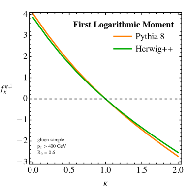
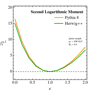
In Fig. 11, we show values of fκg,isuperscriptsubscript𝑓𝜅𝑔𝑖f_{\kappa}^{g,i} extracted from Pythia 8 and Herwig++ for a range of κ𝜅\kappa values. These moments are quite similar between the two parton showers, suggesting that their extraction is robust.
Refer to caption
(a)
Refer to caption
(b)


Figure 11: Extracting the logarithmic moments fκg,1superscriptsubscript𝑓𝜅𝑔1f_{\kappa}^{g,1} (left) and fκg,2superscriptsubscript𝑓𝜅𝑔2f_{\kappa}^{g,2} (right) defined in Eq. (51) from the Pythia 8 and Herwig++ gluon samples.

Like in Ref. Chang:2013iba , we find that logarithmic moments of the nonperturbative function appears in the exponent of the cumulative distribution. Note that the only difference between quark and gluon jets is the color factor Cisubscript𝐶𝑖C_{i}, since the same gluon-based fκg,nsuperscriptsubscript𝑓𝜅𝑔𝑛f_{\kappa}^{g,n} appears for both kinds of jets. Thus, this observable satisfies Casimir scaling in the LL limit, yielding the mutual information discussed in Sec. 3. Strictly speaking, these fκg,nsuperscriptsubscript𝑓𝜅𝑔𝑛f_{\kappa}^{g,n} terms are only relevant at NLL order, since they multiply at most single logarithms in the observable.131313One could imagine power counting fκg,nsuperscriptsubscript𝑓𝜅𝑔𝑛f_{\kappa}^{g,n} as being logarithmically enhanced instead of as 𝒪(1)𝒪1\mathcal{O}(1). In that case, however, one would need to keep track of every fκg,nsuperscriptsubscript𝑓𝜅𝑔𝑛f_{\kappa}^{g,n} starting at NLL order, so we effectively return to the β=0𝛽0\beta=0 case where the full Fκg(x,μ)subscriptsuperscript𝐹𝑔𝜅𝑥𝜇F^{g}_{\kappa}(x,\mu) function is needed. Therefore, we will drop the fκg,nsuperscriptsubscript𝑓𝜅𝑔𝑛f_{\kappa}^{g,n} terms at LL order:

RiLL(λβκ)=αsπCiβκln2λβκ.superscriptsubscript𝑅𝑖LLsubscriptsuperscript𝜆𝜅𝛽subscript𝛼𝑠𝜋subscript𝐶𝑖𝛽𝜅superscript2subscriptsuperscript𝜆𝜅𝛽R_{i}^{\text{LL}}({\lambda^{\kappa}_{\beta}})=\frac{\alpha_{s}}{\pi}\frac{C_{i}}{\beta\kappa}\ln^{2}{\lambda^{\kappa}_{\beta}}. (52)

Doing the full NLL calculation using Eq. (47) is straightforward with the help of two tricks. First, using the fact that

Θ(xzκθβλβκ)=Θ(zθβ/κ(λβκx)1/κ),Θ𝑥superscript𝑧𝜅superscript𝜃𝛽subscriptsuperscript𝜆𝜅𝛽Θ𝑧superscript𝜃𝛽𝜅superscriptsubscriptsuperscript𝜆𝜅𝛽𝑥1𝜅\Theta(xz^{\kappa}\theta^{\beta}-{\lambda^{\kappa}_{\beta}})=\Theta\left(z\theta^{\beta/\kappa}-\left(\frac{{\lambda^{\kappa}_{\beta}}}{x}\right)^{1/\kappa}\right), (53)

we can rewrite the radiator function in Eq. (46) as

Ri(λβκ)=0dxFκg(x,μ)R^i(eβ/κ=(λβκx)1/κ),subscript𝑅𝑖subscriptsuperscript𝜆𝜅𝛽superscriptsubscript0differential-d𝑥subscriptsuperscript𝐹𝑔𝜅𝑥𝜇subscript^𝑅𝑖subscript𝑒𝛽𝜅superscriptsubscriptsuperscript𝜆𝜅𝛽𝑥1𝜅R_{i}({\lambda^{\kappa}_{\beta}})=\int_{0}^{\infty}\!\mathrm{d}x\,F^{g}_{\kappa}(x,\mu)\,\hat{R}_{i}\left({e_{\beta/\kappa}}=\left(\frac{{\lambda^{\kappa}_{\beta}}}{x}\right)^{1/\kappa}\right), (54)

where R^isubscript^𝑅𝑖\hat{R}_{i} is the radiator for the IRC safe angularity with exponent β/κ𝛽𝜅\beta/\kappa. Second, we only need to keep the first logarithmic moment fκg,1superscriptsubscript𝑓𝜅𝑔1f_{\kappa}^{g,1} at NLL order, so when we do the x𝑥x integral weighted by Fκg(x,μ)subscriptsuperscript𝐹𝑔𝜅𝑥𝜇F^{g}_{\kappa}(x,\mu), we can effectively replace

xexp(fκg,1)𝑥superscriptsubscript𝑓𝜅𝑔1x\to\exp(f_{\kappa}^{g,1}) (55)

in the argument of R^isubscript^𝑅𝑖\hat{R}_{i}, up to log-suppressed terms.141414Note that this rescaling would replace fκg,2superscriptsubscript𝑓𝜅𝑔2f_{\kappa}^{g,2} with (fκg,1)2superscriptsuperscriptsubscript𝑓𝜅𝑔12(f_{\kappa}^{g,1})^{2} in Eq. (50). Because the fκg,2superscriptsubscript𝑓𝜅𝑔2f_{\kappa}^{g,2} term is formally beyond NLL accuracy, this is an allowed replacement. Thus, the IRC unsafe radiator is simply

RiNLL(λβκ)=R^iNLL(eβ/κ=(λβκexp(fκg,1))1/κ),superscriptsubscript𝑅𝑖NLLsubscriptsuperscript𝜆𝜅𝛽superscriptsubscript^𝑅𝑖NLLsubscript𝑒𝛽𝜅superscriptsubscriptsuperscript𝜆𝜅𝛽superscriptsubscript𝑓𝜅𝑔11𝜅R_{i}^{\text{NLL}}({\lambda^{\kappa}_{\beta}})=\hat{R}_{i}^{\text{NLL}}\left({e_{\beta/\kappa}}=\left(\frac{{\lambda^{\kappa}_{\beta}}}{\exp(f_{\kappa}^{g,1})}\right)^{1/\kappa}\right), (56)

where the IRC safe radiator R^isubscript^𝑅𝑖\hat{R}_{i} is given in App. B.1. We find it quite remarkable that we can relate an IRC unsafe distribution to an IRC safe one in this way, and we show that these same two tricks are valid in SCET in App. C.1.151515It is perhaps even more remarkable that we can take logarithmic derivatives of the resulting Risubscript𝑅𝑖R_{i} and get the right NLL expression for the multiple emissions piece. Ultimately, the only way we are able to justify this is via SCET, since the original CAESAR approach was only proven for IRC safe observables. Note that there is a Jacobian factor in Risubscriptsuperscript𝑅𝑖R^{\prime}_{i}, so you cannot directly relate the cumulative distributions for eβ/κsubscript𝑒𝛽𝜅{e_{\beta/\kappa}} and λβκ/exp(fκg,1)subscriptsuperscript𝜆𝜅𝛽superscriptsubscript𝑓𝜅𝑔1{\lambda^{\kappa}_{\beta}}/\exp(f_{\kappa}^{g,1}), only the radiators. Because of the Risubscriptsuperscript𝑅𝑖R^{\prime}_{i} term, the discrimination power is not just a function of β/κ𝛽𝜅\beta/\kappa, and has non-trivial κ𝜅\kappa and fκg,1superscriptsubscript𝑓𝜅𝑔1f_{\kappa}^{g,1} dependence at NLL.

Before showing analytic results, we need to comment on the range of validity of our calculation. Because the radiator scales like 1/(βκ)1𝛽𝜅1/(\beta\kappa), we can only trust this perturbative expression when βκ0.5greater-than-or-equivalent-to𝛽𝜅0.5\beta\kappa\gtrsim 0.5. In addition, the validity of our approach is limited to the region where, in absolute terms, the nonperturbative parameter fκg,1superscriptsubscript𝑓𝜅𝑔1f_{\kappa}^{g,1} is smaller than the typical values of lnλβκsubscriptsuperscript𝜆𝜅𝛽\ln{\lambda^{\kappa}_{\beta}}.161616Outside of this region, the nonperturbative effects become too large to be treated using just the logarithmic moments, and we would have to include the full Fκg(x,μ)subscriptsuperscript𝐹𝑔𝜅𝑥𝜇F^{g}_{\kappa}(x,\mu) function, as also mentioned in footnote 13. In principle, this would allow us to get beyond the “nonperturbative barrier” in Eq. (57), though we have not attempted such a calculation. From Fig. 11 we obtain the approximation fκg,13(1κ)superscriptsubscript𝑓𝜅𝑔131𝜅f_{\kappa}^{g,1}\approx 3(1-\kappa), and using Eq. (52), we expect the distribution to peak at ln2λβκ=βκ/(2αsCi)superscript2subscriptsuperscript𝜆𝜅𝛽𝛽𝜅2subscript𝛼𝑠subscript𝐶𝑖\ln^{2}{\lambda^{\kappa}_{\beta}}=\beta\kappa/(2\alpha_{s}C_{i}). This suggests that our calculation holds for

βκ(1κ)2>c,𝛽𝜅superscript1𝜅2𝑐\frac{\beta\kappa}{(1-\kappa)^{2}}>c, (57)

where c=18αsCi𝑐18subscript𝛼𝑠subscript𝐶𝑖c=18\alpha_{s}C_{i}, which is 2.7similar-to-or-equalsabsent2.7\simeq 2.7 for quarks and 6.0similar-to-or-equalsabsent6.0\simeq 6.0 for gluons. We take the more restrictive value c=6.0𝑐6.0c=6.0 when assessing the validity of the quark/gluon truth overlap, and this is the reason why the blue region in Fig. 7 is missing the upper left and lower right corners.
Refer to caption
(a)
Refer to caption
(b)
Refer to caption
(c)
Refer to caption
(d)
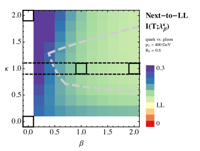
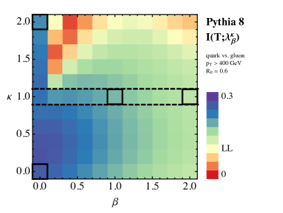
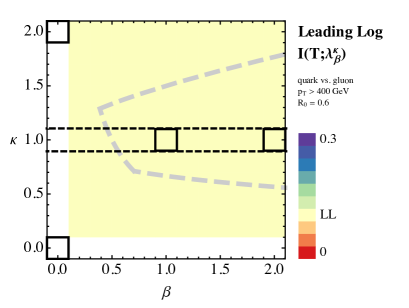
Figure 12: The quark/gluon truth overlap for an individual generalized angularity λβκsubscriptsuperscript𝜆𝜅𝛽{\lambda^{\kappa}_{\beta}}. Top: the LL and NLL analytic calculations. Note that these calculations are singular at κ=0𝜅0\kappa=0 or β=0𝛽0\beta=0. Bottom: the Pythia 8 and Herwig++ parton showers (identical to Figs. 4a and 4b). The solid boxes correspond to dots indicated in Fig. 1, the dashed box corresponds to the IRC safe angularities eβsubscript𝑒𝛽e_{\beta}, and the grey dashed curve in the LL/NLL plots marks the range of validity of our calculations (i.e. the edge of the blue region in Fig. 7).

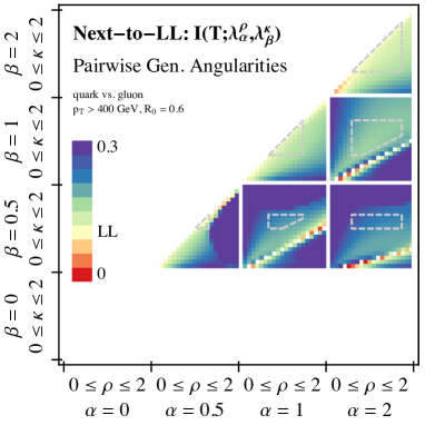
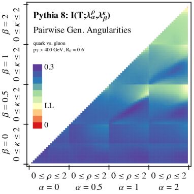
In Fig. 12, we show the truth overlap I(T;λβκ)𝐼𝑇subscriptsuperscript𝜆𝜅𝛽I(T;{\lambda^{\kappa}_{\beta}}), comparing LL, NLL, Pythia 8, and Herwig++. As expected, there is no difference between different choices of κ𝜅\kappa and β𝛽\beta at LL, with differences showing up first at NLL order. The NLL calculation breaks down in the upper left region (due to large values of fκg,1superscriptsubscript𝑓𝜅𝑔1f_{\kappa}^{g,1}) and in the lower left region (due to βκ𝛽𝜅\beta\kappa being too small). Unfortunately, these are exactly the same regions where there is interesting behavior in the Pythia 8 and Herwig++ predictions. If we naively trust the NLL results outside of their range of validity, then starting from broadening (λ11subscriptsuperscript𝜆11{\lambda^{1}_{1}}) and approaching multiplicity (λ00subscriptsuperscript𝜆00{\lambda^{0}_{0}}), the NLL results show an increase in discrimination power, in agreement with the parton showers. However approaching pTDsuperscriptsubscript𝑝𝑇𝐷p_{T}^{D} (λ02subscriptsuperscript𝜆20{\lambda^{2}_{0}}), the NLL results also show an increase in discrimination power, which is the opposite behavior from the parton showers (until one reaches the actual β=0𝛽0\beta=0 line). Of course, one should be wary of this extrapolation, since our calculations are lacking important nonperturbative corrections.171717Intuitively, the parton shower results make sense. Compared to gluons, quarks typically have smaller values of λ11subscriptsuperscript𝜆11{\lambda^{1}_{1}} but larger values of λ02subscriptsuperscript𝜆20{\lambda^{2}_{0}}. Thus, interpolating between λ11subscriptsuperscript𝜆11{\lambda^{1}_{1}} and λ02subscriptsuperscript𝜆20{\lambda^{2}_{0}} should yield a poor discriminant variable. In the NLL approach, small β𝛽\beta is always favored, and calculational control is lost before the fκg,1superscriptsubscript𝑓𝜅𝑔1f_{\kappa}^{g,1} parameter has a chance to reverse that trend.

6.3 Two β>0𝛽0\beta>0 Angularities

Because the resummed λβκsubscriptsuperscript𝜆𝜅𝛽{\lambda^{\kappa}_{\beta}} distributions for β>0𝛽0\beta>0 only depend on logarithmic moments of the weighted-energy function, we have an opportunity to analytically study the correlations between two generalized angularities λαρsubscriptsuperscript𝜆𝜌𝛼{\lambda^{\rho}_{\alpha}} and λβκsubscriptsuperscript𝜆𝜅𝛽{\lambda^{\kappa}_{\beta}}. We can already gain a lot of insight from a LL study, and we can use the same tricks as for Eq. (56) to obtain an NLL result.

With the help of the double weighted-energy function in Eq. (42), we can define a double radiator function

Ri(λαρ,λβκ)subscript𝑅𝑖subscriptsuperscript𝜆𝜌𝛼subscriptsuperscript𝜆𝜅𝛽\displaystyle R_{i}({\lambda^{\rho}_{\alpha}},{\lambda^{\kappa}_{\beta}}) =01dθθ01dzαs(pTzθ)πPiig(z)01dx101dx2Fρ,κg(x1,x2;μ)absentsuperscriptsubscript01d𝜃𝜃superscriptsubscript01differential-d𝑧subscript𝛼𝑠subscript𝑝𝑇𝑧𝜃𝜋subscript𝑃𝑖𝑖𝑔𝑧superscriptsubscript01differential-dsubscript𝑥1superscriptsubscript01differential-dsubscript𝑥2subscriptsuperscript𝐹𝑔𝜌𝜅subscript𝑥1subscript𝑥2𝜇\displaystyle=\int_{0}^{1}\frac{\mathrm{d}\theta}{\theta}\int_{0}^{1}\!\mathrm{d}z\,\frac{\alpha_{s}(p_{T}z\theta)}{\pi}P_{i\to ig}(z)\int_{0}^{1}\!\mathrm{d}x_{1}\int_{0}^{1}\!\mathrm{d}x_{2}\,F^{g}_{\rho,\kappa}(x_{1},x_{2};\mu)
×[1Θ(λαρx1zρθα)Θ(λβκx2zκθβ)].absentdelimited-[]1Θsubscriptsuperscript𝜆𝜌𝛼subscript𝑥1superscript𝑧𝜌superscript𝜃𝛼Θsubscriptsuperscript𝜆𝜅𝛽subscript𝑥2superscript𝑧𝜅superscript𝜃𝛽\displaystyle\qquad\times\left[1-\Theta({\lambda^{\rho}_{\alpha}}-x_{1}z^{\rho}\theta^{\alpha})\Theta({\lambda^{\kappa}_{\beta}}-x_{2}z^{\kappa}\theta^{\beta})\right]. (58)

Again assuming that Fρ,κgsubscriptsuperscript𝐹𝑔𝜌𝜅F^{g}_{\rho,\kappa} does not have any large hierarchies (such that the observables are dominated by the hardest emissions), then we can follow the logic of Ref. Larkoski:2013paa and say that at LL accuracy

1σid2σidλαρdλβκ=(2λαρλβκeRi(λαρ,λβκ))Θ0(λαρ,λβκ),1subscript𝜎𝑖superscriptd2subscript𝜎𝑖dsubscriptsuperscript𝜆𝜌𝛼dsubscriptsuperscript𝜆𝜅𝛽superscript2subscriptsuperscript𝜆𝜌𝛼subscriptsuperscript𝜆𝜅𝛽superscript𝑒subscript𝑅𝑖subscriptsuperscript𝜆𝜌𝛼subscriptsuperscript𝜆𝜅𝛽subscriptΘ0subscriptsuperscript𝜆𝜌𝛼subscriptsuperscript𝜆𝜅𝛽\frac{1}{\sigma_{i}}\frac{\mathrm{d}^{2}\sigma_{i}}{\mathrm{d}{\lambda^{\rho}_{\alpha}}\,\mathrm{d}{\lambda^{\kappa}_{\beta}}}=\left(\frac{\partial^{2}}{\partial{\lambda^{\rho}_{\alpha}}\,\partial{\lambda^{\kappa}_{\beta}}}e^{-R_{i}({\lambda^{\rho}_{\alpha}},{\lambda^{\kappa}_{\beta}})}\right)\Theta_{0}({\lambda^{\rho}_{\alpha}},{\lambda^{\kappa}_{\beta}}), (59)

where Θ0(λαρ,λβκ)subscriptΘ0subscriptsuperscript𝜆𝜌𝛼subscriptsuperscript𝜆𝜅𝛽\Theta_{0}({\lambda^{\rho}_{\alpha}},{\lambda^{\kappa}_{\beta}}) enforces the phase space restrictions181818These assume that nonperturbative physics do not affect the phase space, which is fine for LL accuracy. At NLL, we use Eq. (69) to adjust the phase space given the first logarithmic moments of the weighted-energy function.

((λαρ)κ(λβκ)ρ)sign(α/ρβ/κ)1,((λβκ)α(λαρ)β)sign(α/ρβ/κ)1.formulae-sequencesuperscriptsuperscriptsubscriptsuperscript𝜆𝜌𝛼𝜅superscriptsubscriptsuperscript𝜆𝜅𝛽𝜌sign𝛼𝜌𝛽𝜅1superscriptsuperscriptsubscriptsuperscript𝜆𝜅𝛽𝛼superscriptsubscriptsuperscript𝜆𝜌𝛼𝛽sign𝛼𝜌𝛽𝜅1\left(\frac{({\lambda^{\rho}_{\alpha}})^{\kappa}}{({\lambda^{\kappa}_{\beta}})^{\rho}}\right)^{\text{sign}(\alpha/\rho-\beta/\kappa)}\leq 1,\qquad\left(\frac{({\lambda^{\kappa}_{\beta}})^{\alpha}}{({\lambda^{\rho}_{\alpha}})^{\beta}}\right)^{\text{sign}(\alpha/\rho-\beta/\kappa)}\leq 1. (60)

This expression does not immediately generalize to NLL accuracy, since there is no (known) factorization theorem for double differential distributions over the full phase space. Instead we will exploit the interpolation technique of Ref. Larkoski:2014tva to help find the NLL expression, as we did in Sec. 5.2.

Calculating the double radiator in the LL limit, we find for α/ρ>β/κ𝛼𝜌𝛽𝜅\alpha/\rho>\beta/\kappa

R(λαρ,λβκ)𝑅subscriptsuperscript𝜆𝜌𝛼subscriptsuperscript𝜆𝜅𝛽\displaystyle R({\lambda^{\rho}_{\alpha}},{\lambda^{\kappa}_{\beta}}) LLαsπCiακβρdx1dx2Fρ,κg(x1,x2;μ)(αβln2λβκx2+κρln2λαρx12lnλβκx2lnλαρx1)superscriptsimilar-to-or-equalsLLabsentsubscript𝛼𝑠𝜋subscript𝐶𝑖𝛼𝜅𝛽𝜌differential-dsubscript𝑥1differential-dsubscript𝑥2subscriptsuperscript𝐹𝑔𝜌𝜅subscript𝑥1subscript𝑥2𝜇𝛼𝛽superscript2subscriptsuperscript𝜆𝜅𝛽subscript𝑥2𝜅𝜌superscript2subscriptsuperscript𝜆𝜌𝛼subscript𝑥12subscriptsuperscript𝜆𝜅𝛽subscript𝑥2subscriptsuperscript𝜆𝜌𝛼subscript𝑥1\displaystyle\stackrel{{\scriptstyle\text{LL}}}{{\simeq}}\frac{\alpha_{s}}{\pi}\frac{C_{i}}{\alpha\kappa-\beta\rho}\int\mathrm{d}x_{1}\,\mathrm{d}x_{2}\,F^{g}_{\rho,\kappa}(x_{1},x_{2};\mu)\,\left(\frac{\alpha}{\beta}\ln^{2}\frac{{\lambda^{\kappa}_{\beta}}}{x_{2}}+\frac{\kappa}{\rho}\ln^{2}\frac{{\lambda^{\rho}_{\alpha}}}{x_{1}}-2\ln\frac{{\lambda^{\kappa}_{\beta}}}{x_{2}}\ln\frac{{\lambda^{\rho}_{\alpha}}}{x_{1}}\right)
=αsπCiακβρ[αβ(ln2λβκ2fκg,1lnλβκ+fκg,2)+κρ(ln2λαρ2fρg,1lnλαρ+fρg,2)\displaystyle=\frac{\alpha_{s}}{\pi}\frac{C_{i}}{\alpha\kappa-\beta\rho}\Bigl{[}\frac{\alpha}{\beta}\left(\ln^{2}{\lambda^{\kappa}_{\beta}}-2f_{\kappa}^{g,1}\ln{\lambda^{\kappa}_{\beta}}+f_{\kappa}^{g,2}\right)+\frac{\kappa}{\rho}\left(\ln^{2}{\lambda^{\rho}_{\alpha}}-2f_{\rho}^{g,1}\ln{\lambda^{\rho}_{\alpha}}+f_{\rho}^{g,2}\right)
2(lnλβκlnλαρfκg,1lnλαρfρg,1lnλβκ+fρ,κg,1,1)],\displaystyle\qquad\qquad-2\left(\ln{\lambda^{\kappa}_{\beta}}\ln{\lambda^{\rho}_{\alpha}}-f_{\kappa}^{g,1}\ln{\lambda^{\rho}_{\alpha}}-f_{\rho}^{g,1}\ln{\lambda^{\kappa}_{\beta}}+f_{\rho,\kappa}^{g,1,1}\right)\Bigr{]}, (61)

where we have used Eq. (44) to simplify the last line (accurate to leading power in λαρsubscriptsuperscript𝜆𝜌𝛼{\lambda^{\rho}_{\alpha}} and λβκsubscriptsuperscript𝜆𝜅𝛽{\lambda^{\kappa}_{\beta}}) and we have defined

fρ,κg,1,1=dx1dx2Fρ,κg(x1,x2;μ)lnx1lnx2.superscriptsubscript𝑓𝜌𝜅𝑔11differential-dsubscript𝑥1differential-dsubscript𝑥2subscriptsuperscript𝐹𝑔𝜌𝜅subscript𝑥1subscript𝑥2𝜇subscript𝑥1subscript𝑥2f_{\rho,\kappa}^{g,1,1}=\int\mathrm{d}x_{1}\,\mathrm{d}x_{2}\,F^{g}_{\rho,\kappa}(x_{1},x_{2};\mu)\ln x_{1}\ln x_{2}. (62)

As in the case of a single λβκsubscriptsuperscript𝜆𝜅𝛽{\lambda^{\kappa}_{\beta}}, strictly speaking the nonperturbative parameters fρ,κg,nsuperscriptsubscript𝑓𝜌𝜅𝑔𝑛f_{\rho,\kappa}^{g,n} only show up at subleading logarithmic order, and can be ignored to LL accuracy,

RiLL(λαρ,λβκ)=αsπCiακβρ(αβln2λβκ+κρln2λαρ2lnλβκlnλαρ).superscriptsubscript𝑅𝑖LLsubscriptsuperscript𝜆𝜌𝛼subscriptsuperscript𝜆𝜅𝛽subscript𝛼𝑠𝜋subscript𝐶𝑖𝛼𝜅𝛽𝜌𝛼𝛽superscript2subscriptsuperscript𝜆𝜅𝛽𝜅𝜌superscript2subscriptsuperscript𝜆𝜌𝛼2subscriptsuperscript𝜆𝜅𝛽subscriptsuperscript𝜆𝜌𝛼R_{i}^{\rm LL}({\lambda^{\rho}_{\alpha}},{\lambda^{\kappa}_{\beta}})=\frac{\alpha_{s}}{\pi}\frac{C_{i}}{\alpha\kappa-\beta\rho}\left(\frac{\alpha}{\beta}\ln^{2}{\lambda^{\kappa}_{\beta}}+\frac{\kappa}{\rho}\ln^{2}{\lambda^{\rho}_{\alpha}}-2\ln{\lambda^{\kappa}_{\beta}}\ln{\lambda^{\rho}_{\alpha}}\right). (63)

Note that the exponents ρ𝜌\rho and κ𝜅\kappa still have an effect on the discrimination power even though we are not accounting for the nonperturbative parameters at this order. The overall prefactor implies that when α𝛼\alpha and β𝛽\beta are sufficiently different, we should only trust this distribution for

ακβρ0.5.greater-than-or-equivalent-to𝛼𝜅𝛽𝜌0.5\alpha\kappa-\beta\rho\gtrsim 0.5. (64)

To achieve NLL accuracy, we need to combine the interpolation technique of Ref. Larkoski:2014tva with the two tricks as we used to find the single generalized angularity distribution in Eq. (56). Following Ref. Larkoski:2014tva , we take the following ansatz for the NLL distribution:

Σi(λαρ,λβκ)=eγER~i(λαρ,λβκ)Γ(1+R~i(λαρ,λβκ))eRi(λαρ,λβκ),subscriptΣ𝑖subscriptsuperscript𝜆𝜌𝛼subscriptsuperscript𝜆𝜅𝛽superscript𝑒subscript𝛾𝐸subscript~𝑅𝑖subscriptsuperscript𝜆𝜌𝛼subscriptsuperscript𝜆𝜅𝛽Γ1subscript~𝑅𝑖subscriptsuperscript𝜆𝜌𝛼subscriptsuperscript𝜆𝜅𝛽superscript𝑒subscript𝑅𝑖subscriptsuperscript𝜆𝜌𝛼subscriptsuperscript𝜆𝜅𝛽\Sigma_{i}({\lambda^{\rho}_{\alpha}},{\lambda^{\kappa}_{\beta}})=\frac{e^{-\gamma_{E}\widetilde{R}_{i}({\lambda^{\rho}_{\alpha}},{\lambda^{\kappa}_{\beta}})}}{\Gamma(1+\widetilde{R}_{i}({\lambda^{\rho}_{\alpha}},{\lambda^{\kappa}_{\beta}}))}\,e^{-R_{i}({\lambda^{\rho}_{\alpha}},{\lambda^{\kappa}_{\beta}})}, (65)

where Risubscript𝑅𝑖R_{i} is the double radiator from Eq. (6.3) and R~isubscript~𝑅𝑖\widetilde{R}_{i} is a multiple emissions term that is not given by any simple logarithmic derivative of Risubscript𝑅𝑖R_{i}. We start by considering the double radiator Risubscript𝑅𝑖R_{i}. Looking at the theta functions in Eq. (6.3), we see that the integration range for the double radiator is the same as for two IRC safe angularities with

eα/ρ=(λαρx1)1/ρ,eβ/κ=(λβκx2)1/κ.formulae-sequencesubscript𝑒𝛼𝜌superscriptsubscriptsuperscript𝜆𝜌𝛼subscript𝑥11𝜌subscript𝑒𝛽𝜅superscriptsubscriptsuperscript𝜆𝜅𝛽subscript𝑥21𝜅e_{\alpha/\rho}=\left(\frac{{\lambda^{\rho}_{\alpha}}}{x_{1}}\right)^{1/\rho},\qquad e_{\beta/\kappa}=\left(\frac{{\lambda^{\kappa}_{\beta}}}{x_{2}}\right)^{1/\kappa}. (66)

At NLL accuracy, we only need the first logarithmic moments of the weighted-energy function, so we can make the replacement

x1exp(fρg,1),x2exp(fκg,1).formulae-sequencesubscript𝑥1superscriptsubscript𝑓𝜌𝑔1subscript𝑥2superscriptsubscript𝑓𝜅𝑔1x_{1}\to\exp(f_{\rho}^{g,1}),\qquad x_{2}\to\exp(f_{\kappa}^{g,1}). (67)

Thus, the double radiator is

RiNLL(λαρ,λβκ)=R^iNLL(eα/ρ=(λαρexp(fρg,1))1/ρ,eβ/κ=(λβκexp(fκg,1))1/κ),superscriptsubscript𝑅𝑖NLLsubscriptsuperscript𝜆𝜌𝛼subscriptsuperscript𝜆𝜅𝛽superscriptsubscript^𝑅𝑖NLLformulae-sequencesubscript𝑒𝛼𝜌superscriptsubscriptsuperscript𝜆𝜌𝛼superscriptsubscript𝑓𝜌𝑔11𝜌subscript𝑒𝛽𝜅superscriptsubscriptsuperscript𝜆𝜅𝛽superscriptsubscript𝑓𝜅𝑔11𝜅R_{i}^{\rm NLL}({\lambda^{\rho}_{\alpha}},{\lambda^{\kappa}_{\beta}})=\hat{R}_{i}^{\rm NLL}\left(e_{\alpha/\rho}=\left(\frac{{\lambda^{\rho}_{\alpha}}}{\exp(f_{\rho}^{g,1})}\right)^{1/\rho},\,e_{\beta/\kappa}=\left(\frac{{\lambda^{\kappa}_{\beta}}}{\exp(f_{\kappa}^{g,1})}\right)^{1/\kappa}\right), (68)

where R^iNLLsuperscriptsubscript^𝑅𝑖NLL\hat{R}_{i}^{\rm NLL} is the IRC safe double cumulative distribution for angularities with exponents α/ρ𝛼𝜌\alpha/\rho and β/κ𝛽𝜅\beta/\kappa, defined in App. B.2. Turning to the multiple emissions term R~isubscript~𝑅𝑖\widetilde{R}_{i}, we need to find a function that interpolates between the logarithmic derivative functions R(λαρ)superscript𝑅subscriptsuperscript𝜆𝜌𝛼R^{\prime}({\lambda^{\rho}_{\alpha}}) and R(λβκ)superscript𝑅subscriptsuperscript𝜆𝜅𝛽R^{\prime}({\lambda^{\kappa}_{\beta}}) on the boundaries of phase space. Since we already found the single radiator to NLL accuracy in Eq. (56), this interpolation is straightforward, and we give the explicit expressions in App. B.3. Finally, to have a properly normalized distribution, we have to apply the rescaling

λαρλαρexp(fρg,1),λβκλβκexp(fκg,1)formulae-sequencesubscriptsuperscript𝜆𝜌𝛼subscriptsuperscript𝜆𝜌𝛼superscriptsubscript𝑓𝜌𝑔1subscriptsuperscript𝜆𝜅𝛽subscriptsuperscript𝜆𝜅𝛽superscriptsubscript𝑓𝜅𝑔1{\lambda^{\rho}_{\alpha}}\to\frac{{\lambda^{\rho}_{\alpha}}}{\exp(f_{\rho}^{g,1})},\qquad{\lambda^{\kappa}_{\beta}}\to\frac{{\lambda^{\kappa}_{\beta}}}{\exp(f_{\kappa}^{g,1})} (69)

to the phase space constraints in Eq. (60) as well. Again, we find it remarkable that there is such a close relationship between IRC safe and IRC unsafe calculations at NLL order, and we validate this method in SCET in App. C.2.
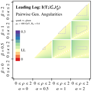
Refer to caption
(a)
Refer to caption
(b)


Refer to caption
(c)
Refer to caption
(d)


Figure 13: The quark/gluon truth overlap for pairs of generalized angularities (λαρ,λβκ)subscriptsuperscript𝜆𝜌𝛼subscriptsuperscript𝜆𝜅𝛽({\lambda^{\rho}_{\alpha}},{\lambda^{\kappa}_{\beta}}). Top: the LL and NLL analytic calculations. Bottom: the Pythia 8 and Herwig++ parton showers. Here, we show four values of β{0,0.5,1,2}𝛽00.512\beta\in\{0,0.5,1,2\} and for each value of β𝛽\beta, 0κ20𝜅20\leq\kappa\leq 2 in steps of size 0.10.10.1. In the NLL and NLL plots, the interior of the dashed grey boxes correspond to the range of validity of our calculations.

In Fig. 13, we show the truth overlap for the LL and NLL calculations, compared to results obtained from Pythia 8 and Herwig++. The LL and NLL calculations do not extend to the region where α𝛼\alpha or β𝛽\beta is zero, which are left white in the plot. We caution the reader that some of these LL and NLL results extrapolate outside the range of validity in Eqs. (57) and (64). Comparing the various predictions, we observe similarities between the regions of minimal and maximal discrimination power, though the overall discrimination power is (again) larger for Pythia 8 and NLL than for Herwig++ and LL. The Pythia 8 and NLL results most clearly indicate that it is advantageous to pick one of the angular exponents α𝛼\alpha or β𝛽\beta to be small. A notable difference between the predictions is that the LL and NLL calculations suggest that one should avoid the diagonal ρ=κ𝜌𝜅\rho=\kappa, whereas for Pythia 8, and to a lesser extent Herwig++, the maximum discrimination power is sometimes (surprisingly) close to it (see e.g. α=1𝛼1\alpha=1, β=0.5𝛽0.5\beta=0.5).

7 Conclusions

Robust quark/gluon discrimination is a key goal for the jet substructure community, so to the extent possible, it is important to use first principles calculations to assess the challenges and opportunities. In this paper, we showed that mutual information is a powerful way to understand how variables are correlated, and whether or not that (lack of) correlation pertains to discrimination power. We also made progress in gaining analytic control over the tagging performance of the generalized angularities λβκsubscriptsuperscript𝜆𝜅𝛽{\lambda^{\kappa}_{\beta}}. For the IRC safe angularities and the IRC unsafe angularities with β>0𝛽0\beta>0, we calculated the quark/gluon truth overlap for a single angularity I(T;λβκ)𝐼𝑇subscriptsuperscript𝜆𝜅𝛽I(T;{\lambda^{\kappa}_{\beta}}) and for pairs of angularities I(T;λαρ,λβκ)𝐼𝑇subscriptsuperscript𝜆𝜌𝛼subscriptsuperscript𝜆𝜅𝛽I(T;{\lambda^{\rho}_{\alpha}},{\lambda^{\kappa}_{\beta}}) to NLL order.

Ultimately, we want to extend our analysis to higher orders, but this would require a robust “truth” definition for a quark jet versus a gluon jet. While the strategy of Ref. Banfi:2006hf is one option to define the truth flavor of a jet, we would prefer a definition for which the jet constituents are the same as for traditional flavor-less jet algorithms. Of course, quark and gluon jets do not exist in isolation, and at some point, the color correlations between the jets will be relevant for characterizing the discrimination power. The techniques introduced recently in Ref. Stewart:2014nna should help in gaining analytic control over those color correlations. Since our NLL results are subject to large changes from scale variation, higher-order calculations will be crucial for robust uncertainty estimates.

Assuming we did have a suitable quark/gluon truth definition, then a key challenge for calculations beyond our present order is dealing with soft radiation, in particular the effect of non-global logarithms Dasgupta:2001sh . One option is to do quark/gluon tagging in concert with soft drop declustering Larkoski:2014wba (a generalization of modified mass drop tagging Butterworth:2008iy ; Dasgupta:2013ihk ). The soft drop procedure removes soft radiation, and therefore removes non-global contributions to the jet. The cumulative distributions for a single soft-dropped angularity were already calculated in Ref. Larkoski:2014wba , where the distributions exhibited Casimir scaling at LL order. Using soft-dropped jet shapes for quark/gluon discrimination seems promising from both a theoretical and experimental point of view, and we leave a more detailed study to future work.

Based on our studies, we have two recommendations to the ATLAS and CMS experiments. The first recommendation is to make (unfolded) measurements of the recoil-free angularities distributions for a range of β𝛽\beta values, ideally in purified quark/gluon samples.191919Initial results along these lines appear in Ref. Aad:2014gea for the energy correlation function ratio C1(β)superscriptsubscript𝐶1𝛽C_{1}^{(\beta)} Larkoski:2013eya , though only the final quark/gluon performance is shown, not the extracted quark and gluon distributions. The differences seen between Monte Carlo programs in Fig. 4 is worrisome, and while eventually calculations might be a guide to what these distributions should look like, in the short term eβsubscript𝑒𝛽{e_{\beta}} measurements can be a key reference for tuning Monte Carlo programs, especially because the differences arise from effects that are formally beyond LL accuracy. The second recommendation is to measure more double differential distributions.202020There are double differential results in Ref. TheATLAScollaboration:2013tia , but measured only in simulation and not in data. While we focused on mutual information with the truth in this paper, one would still like to understand the full correlation structure. Angularities are a good place to start, and double differential distributions of eαsubscript𝑒𝛼{e_{\alpha}} and eβsubscript𝑒𝛽{e_{\beta}} would be quite valuable, especially with new calculational tools available to predict these correlations Larkoski:2013paa ; Larkoski:2014tva ; Procura:2014cba (see App. D for example plots along these lines).

Finally, in the spirit of Refs. Krohn:2012fg ; Waalewijn:2012sv ; Chang:2013rca ; Chang:2013iba , we have provided another example of how collinear unsafe (but soft safe) observables can be made calculable with the help of new nonperturbative objects. We introduced the weighted-energy functions Fκi(x)superscriptsubscript𝐹𝜅𝑖𝑥F_{\kappa}^{i}(x), which allowed us to understand many aspects of the κ1𝜅1\kappa\not=1 regime. Because the β>0𝛽0\beta>0 angularities only depend on logarithmic moments of Fκi(x)superscriptsubscript𝐹𝜅𝑖𝑥F_{\kappa}^{i}(x), they are the simplest to understand. But even the β=0𝛽0\beta=0 angularities are within calculational control, since we can study the renormalization group behavior of, say, the pTDsuperscriptsubscript𝑝𝑇𝐷p_{T}^{D} (λ02subscriptsuperscript𝜆20{\lambda^{2}_{0}}) distribution. Of course, hadron multiplicity (λ00subscriptsuperscript𝜆00{\lambda^{0}_{0}}) is not captured within our framework due to the presence of the soft singularity, but perhaps hadron multiplicities could be made analytically tractable by using soft drop declustering to remove soft radiation. We expect future studies will continue to improve (and improve our understanding of) quark/gluon discrimination.

Acknowledgements.
We thank the participants of the Boost 2013 workshop for many inspiring discussions that led to this work. We also thank Jason Gallicchio, Aram Harrow, and Matthew Headrick for conversations about mutual information and T.J. Wilkason for coding help. A.L. and J.T. are supported by the U.S. Department of Energy (DOE) under cooperative research agreement DE-FG02-05ER-41360. J.T. is also supported by the DOE Early Career research program DE-FG02-11ER-41741 and by a Sloan Research Fellowship from the Alfred P. Sloan Foundation. W.W. is supported by a Marie Curie International Incoming Fellowship within the 7th European Community Framework Program (PIIF-GA-2012-328913).

Appendix A Properties of Mutual Information

A.1 Relationship to the ROC Curve

The mutual information of an observable A𝐴A with the truth T𝑇T can be derived from the ROC curve of A𝐴A. Although we phrase this discussion in terms of quark/gluon discrimination, it obviously carries over to other cases as well.

At the position (q,g)𝑞𝑔(q,g) on the ROC curve, the region dqd𝑞\mathrm{d}q has a fraction dqd𝑞\mathrm{d}q of the quark jets. The fraction of gluon jets is given by the slope of the ROC curve, dgd𝑔\mathrm{d}g = g(q)dqsuperscript𝑔𝑞d𝑞g^{\prime}(q)\,\mathrm{d}q. Looking at the definition of I(T;A)𝐼𝑇𝐴I(T;A) in Eq. (2.2), we can write the integrals as

dapq(a)dq,dapg(a)dg=dqg(q).formulae-sequencedifferential-d𝑎subscript𝑝𝑞𝑎differential-d𝑞differential-d𝑎subscript𝑝𝑔𝑎differential-d𝑔differential-d𝑞superscript𝑔𝑞\int\mathrm{d}a\,p_{q}(a)\Rightarrow\int\mathrm{d}q,\quad\int\mathrm{d}a\,p_{g}(a)\Rightarrow\int\mathrm{d}g=\int\mathrm{d}q\,g^{\prime}(q). (70)

For a sample with quark fraction f𝑓f, the ratios of the probability distributions are

pq(a)ptot(a)dqdqf+dg(1f),pg(a)ptot(a)dgdqf+dg(1f).formulae-sequencesubscript𝑝𝑞𝑎subscript𝑝tot𝑎d𝑞d𝑞𝑓d𝑔1𝑓subscript𝑝𝑔𝑎subscript𝑝tot𝑎d𝑔d𝑞𝑓d𝑔1𝑓\frac{p_{q}(a)}{p_{\rm tot}(a)}\Rightarrow\frac{\mathrm{d}q}{\mathrm{d}qf+\mathrm{d}g(1-f)},\qquad\frac{p_{g}(a)}{p_{\rm tot}(a)}\Rightarrow\frac{\mathrm{d}g}{\mathrm{d}qf+\mathrm{d}g(1-f)}. (71)

This leads to

I(T;A)=dq(flog21f+(1f)g(q)+(1f)g(q)log2g(q)f+(1f)g(q)).𝐼𝑇𝐴differential-d𝑞𝑓subscript21𝑓1𝑓superscript𝑔𝑞1𝑓superscript𝑔𝑞subscript2superscript𝑔𝑞𝑓1𝑓superscript𝑔𝑞I(T;A)=\int\!\mathrm{d}q\,\left(f\,\log_{2}\frac{1}{f+(1-f)g^{\prime}(q)}+(1-f)\,g^{\prime}(q)\log_{2}\frac{g^{\prime}(q)}{f+(1-f)g^{\prime}(q)}\right). (72)

As a simple test of this formula, note that the ROC curve for an observable that satisfies Casimir scaling is g(q)=q(CA/CF)𝑔𝑞superscript𝑞subscript𝐶𝐴subscript𝐶𝐹g(q)=q^{(C_{A}/C_{F})}. Plugging this into Eq. (72), we recover I(T;A)𝐼𝑇𝐴I(T;A) from Eq. (24).

Inverting this relationship to obtain the ROC curve from the mutual information is not so easy, suggesting that mutual information is an easier concept to work with. Nevertheless it seems in principle possible, though we do not claim that the following simple-minded approach is optimal. Consider discretizing g(q)superscript𝑔𝑞g^{\prime}(q) by treating it as a constant gisubscriptsuperscript𝑔𝑖g^{\prime}_{i} on the interval q[i/nbins,(i+1)/nbins]𝑞𝑖subscript𝑛bins𝑖1subscript𝑛binsq\in[i/n_{\text{bins}},(i+1)/n_{\text{bins}}] with i=0,1,,nbins1𝑖01subscript𝑛bins1i=0,1,\dots,n_{\text{bins}}-1. Because an ideal ROC curve is not only monotonically increasing (i.e. g(q)0superscript𝑔𝑞0g^{\prime}(q)\geq 0) but also convex (i.e. g′′(q)0superscript𝑔′′𝑞0g^{\prime\prime}(q)\geq 0), this means that gi+1gisubscriptsuperscript𝑔𝑖1subscriptsuperscript𝑔𝑖g^{\prime}_{i+1}\geq g^{\prime}_{i}, and we have a chance to find a set of equations that (uniquely) determine gisubscriptsuperscript𝑔𝑖g^{\prime}_{i}. Then, we can integrate g(q)superscript𝑔𝑞g^{\prime}(q) in the usual way to find g(q)𝑔𝑞g(q). One set of equations is given by the n𝑛n-th derivative of I(T;A)𝐼𝑇𝐴I(T;A) evaluated at f=1𝑓1f=1 (for n2𝑛2n\geq 2)

dnI(T;A)dfn|f=1=(n2)!ln201dq(g(q)1)n.evaluated-atsuperscriptd𝑛𝐼𝑇𝐴dsuperscript𝑓𝑛𝑓1𝑛22superscriptsubscript01differential-d𝑞superscriptsuperscript𝑔𝑞1𝑛\frac{\mathrm{d}^{n}I(T;A)}{\mathrm{d}f^{n}}\bigg{|}_{f=1}=-\frac{(n-2)!}{\ln 2}\,\int_{0}^{1}\!\mathrm{d}q\,(g^{\prime}(q)-1)^{n}. (73)

while for the special case of n=1𝑛1n=1 we can use

01dq(g(q)1)=0.superscriptsubscript01differential-d𝑞superscript𝑔𝑞10\int_{0}^{1}\!\mathrm{d}q\,(g^{\prime}(q)-1)=0. (74)

In discrete form, these become a system of polynomial equations

1nbinsi(gi1)1subscript𝑛binssubscript𝑖superscriptsubscript𝑔𝑖1\displaystyle\frac{1}{n_{\text{bins}}}\sum_{i}(g_{i}^{\prime}-1) =0,absent0\displaystyle=0,
1nbinsi(gi1)n1subscript𝑛binssubscript𝑖superscriptsuperscriptsubscript𝑔𝑖1𝑛\displaystyle\frac{1}{n_{\text{bins}}}\sum_{i}(g_{i}^{\prime}-1)^{n} =ln2(n2)!dnI(T;A)dfn|f=1.absentevaluated-at2𝑛2superscriptd𝑛𝐼𝑇𝐴dsuperscript𝑓𝑛𝑓1\displaystyle=-\frac{\ln 2}{(n-2)!}\frac{\mathrm{d}^{n}I(T;A)}{\mathrm{d}f^{n}}\bigg{|}_{f=1}\,. (75)

Because these equation are non-linear, this quickly becomes numerically unstable for nbins>4subscript𝑛bins4n_{\text{bins}}>4, but gives a proof of principle that a solution can be found. Note that the condition that the ROC curve is convex is crucial, since otherwise each permutation of gisubscriptsuperscript𝑔𝑖g^{\prime}_{i} would also constitute a solution. For special functional forms, there are simpler strategies to find the ROC curve. For example, if it is known that g(q)=qc𝑔𝑞superscript𝑞𝑐g(q)=q^{c}, then a practical way to estimate the exponent c𝑐c is via

dI(T;A)df|f=0=1ln201dqlng(q)=c1lncln2.evaluated-atd𝐼𝑇𝐴d𝑓𝑓012superscriptsubscript01differential-d𝑞superscript𝑔𝑞𝑐1𝑐2\displaystyle\frac{\mathrm{d}I(T;A)}{\mathrm{d}f}\bigg{|}_{f=0}=-\frac{1}{\ln 2}\int_{0}^{1}\!\mathrm{d}q\,\ln g^{\prime}(q)=\frac{c-1-\ln c}{\ln 2}. (76)

A.2 Better ROC Curve Implies Greater Truth Overlap

When one observable b𝑏b has a larger truth overlap than another observable w𝑤w, i.e.

I(T;B)>I(T;W),𝐼𝑇𝐵𝐼𝑇𝑊I(T;B)>I(T;W), (77)

we interpreted this to mean that b𝑏b is a better discriminant variable and w𝑤w is worse. While this is generically true, there can be cases where the “worse” observable can have better performance at a given operating point. This occurs when the ROC curves of b𝑏b and w𝑤w intersect, for example when b𝑏b has better background rejection at low signal efficiency but w𝑤w performs better at high signal efficiency. Thus, we cannot conclude from the truth overlap alone whether b𝑏b or w𝑤w is better, since even from a ROC curve perspective, “better” is ill-defined.

What we can prove is that if the ROC curve for b𝑏b is everywhere better than for w𝑤w, then the corresponding truth overlap is strictly larger. In information theory language, we would say that b𝑏b is Pareto optimal with respect to w𝑤w. Consider the ROC curves gb(q)subscript𝑔𝑏𝑞g_{b}(q) and gw(q)subscript𝑔𝑤𝑞g_{w}(q). A better observable’s ROC curve will take a smaller value (less background) at each value of signal efficiency. Thus we can define the better observable as

gb(q)gw(q)Δ(q),subscript𝑔𝑏𝑞subscript𝑔𝑤𝑞Δ𝑞g_{b}(q)\equiv g_{w}(q)-\Delta(q), (78)

where Δ(q)0Δ𝑞0\Delta(q)\geq 0 for all q[0,1]𝑞01q\in[0,1]. We will now use a variational method to show that I(T;B)>I(T;W)𝐼𝑇𝐵𝐼𝑇𝑊I(T;B)>I(T;W).

From these two ROC curves, we can calculate the difference between their truth overlaps. Using the relationship between mutual information and the ROC curve from Eq. (72) we have:

I(T;B)I(T;W)𝐼𝑇𝐵𝐼𝑇𝑊\displaystyle I(T;B)-I(T;W) =dq(flog21f+(1f)gb(q)+(1f)gb(q)log2gb(q)f+(1f)gb(q))absentdifferential-d𝑞𝑓subscript21𝑓1𝑓superscriptsubscript𝑔𝑏𝑞1𝑓superscriptsubscript𝑔𝑏𝑞subscript2superscriptsubscript𝑔𝑏𝑞𝑓1𝑓superscriptsubscript𝑔𝑏𝑞\displaystyle=\int\!\mathrm{d}q\,\left(f\,\log_{2}\frac{1}{f+(1-f)g_{b}^{\prime}(q)}+(1-f)\,g_{b}^{\prime}(q)\log_{2}\frac{g_{b}^{\prime}(q)}{f+(1-f)g_{b}^{\prime}(q)}\right)
dq(flog21f+(1f)gw(q)+(1f)gw(q)log2gw(q)f+(1f)gw(q))differential-d𝑞𝑓subscript21𝑓1𝑓superscriptsubscript𝑔𝑤𝑞1𝑓superscriptsubscript𝑔𝑤𝑞subscript2superscriptsubscript𝑔𝑤𝑞𝑓1𝑓superscriptsubscript𝑔𝑤𝑞\displaystyle-\int\!\mathrm{d}q\,\left(f\,\log_{2}\frac{1}{f+(1-f)g_{w}^{\prime}(q)}+(1-f)\,g_{w}^{\prime}(q)\log_{2}\frac{g_{w}^{\prime}(q)}{f+(1-f)g_{w}^{\prime}(q)}\right)
=𝑑qΔ(q)log2(1f)gw(q)f+(1f)gw(q)+𝒪(Δ2).absentdifferential-d𝑞superscriptΔ𝑞subscript21𝑓superscriptsubscript𝑔𝑤𝑞𝑓1𝑓superscriptsubscript𝑔𝑤𝑞𝒪superscriptΔ2\displaystyle=-\,\int\!dq\,\Delta^{\prime}(q)\log_{2}\frac{(1-f)g_{w}^{\prime}(q)}{f+(1-f)g_{w}^{\prime}(q)}+{\cal O}(\Delta^{2})\,. (79)

In the last step, we expanded the integrand assuming that Δ(q)Δ𝑞\Delta(q) is small. Because any ROC curve g𝑔g must satisfy g(0)=0𝑔00g(0)=0 and g(1)=1𝑔11g(1)=1, we can perform integration by parts on Δ(q)superscriptΔ𝑞\Delta^{\prime}(q) without introducing any boundary terms.

I(T;B)I(T;W)𝐼𝑇𝐵𝐼𝑇𝑊\displaystyle I(T;B)-I(T;W) =1ln2𝑑qΔ(q)gw′′(q)gw(q)f(1f)f+(1f)gw(q)+𝒪(Δ2).absent12differential-d𝑞Δ𝑞superscriptsubscript𝑔𝑤′′𝑞superscriptsubscript𝑔𝑤𝑞𝑓1𝑓𝑓1𝑓superscriptsubscript𝑔𝑤𝑞𝒪superscriptΔ2\displaystyle=\frac{1}{\ln 2}\int\!dq\,\Delta(q)\frac{g_{w}^{\prime\prime}(q)}{g_{w}^{\prime}(q)}\frac{f(1-f)}{f+(1-f)g_{w}^{\prime}(q)}+{\cal O}(\Delta^{2})\,. (80)

This term is manifestly positive because for any (ideal) ROC curve g(q)0superscript𝑔𝑞0g^{\prime}(q)\geq 0 and g′′(q)0superscript𝑔′′𝑞0g^{\prime\prime}(q)\geq 0 for all q[0,1]𝑞01q\in[0,1], and Δ(q)Δ𝑞\Delta(q) is positive by assumption. Therefore,

I(T;B)I(T;W)>0𝐼𝑇𝐵𝐼𝑇𝑊0\displaystyle I(T;B)-I(T;W)>0\, (81)

up to corrections of order Δ2superscriptΔ2\Delta^{2}. However, we can make these Δ2superscriptΔ2\Delta^{2} corrections arbitrarily small by applying this variational logic to a sequence of ROC curves that smoothly interpolate between gb(q)subscript𝑔𝑏𝑞g_{b}(q) and gw(q)subscript𝑔𝑤𝑞g_{w}(q).212121Concretely, one can always build an interpolating strategy based on randomly selecting b𝑏b or w𝑤w as the discriminant variable with predetermined probability. Thus, we have proven that an observable with an everywhere-better ROC curve also has a larger truth overlap.

A.3 Subtleties of Finite Statistics and Binning

When dealing with a sample with a finite number of events, the Shannon entropy H𝐻H is sensitive to the way in which the sample is binned. We will compute the leading effect this has on the entropy. Let Nbinssubscript𝑁binsN_{\text{bins}} be the number of bins and let λisubscript𝜆𝑖\lambda_{i} be the average number of events in bin i𝑖i. The total number of events in the sample is

i=1Nbinsλi=Nev.superscriptsubscript𝑖1subscript𝑁binssubscript𝜆𝑖subscript𝑁ev\sum_{i=1}^{N_{\text{bins}}}\lambda_{i}=N_{\text{ev}}. (82)

For sufficiently large Nevsubscript𝑁evN_{\text{ev}}, the fluctuations within the bins should be independent and the number of events in bin i𝑖i should be Poisson distributed about λisubscript𝜆𝑖\lambda_{i}. Thus, the expected entropy of the binned sample is

H=i=1Nbinsni=0λinieλini!(niNevlog2niNev),𝐻superscriptsubscript𝑖1subscript𝑁binssuperscriptsubscriptsubscript𝑛𝑖0superscriptsubscript𝜆𝑖subscript𝑛𝑖superscript𝑒subscript𝜆𝑖subscript𝑛𝑖subscript𝑛𝑖subscript𝑁evsubscript2subscript𝑛𝑖subscript𝑁evH=\sum_{i=1}^{N_{\text{bins}}}\sum_{n_{i}=0}^{\infty}\frac{\lambda_{i}^{n_{i}}e^{-\lambda_{i}}}{n_{i}!}\left(-\frac{n_{i}}{N_{\text{ev}}}\log_{2}\frac{n_{i}}{N_{\text{ev}}}\right), (83)

where nisubscript𝑛𝑖n_{i} ranges over the possible observed events in bin i𝑖i.

Assuming that λi1much-greater-thansubscript𝜆𝑖1\lambda_{i}\gg 1 for all bins, we can expand the entropy about the average value ni=λidelimited-⟨⟩subscript𝑛𝑖subscript𝜆𝑖\langle n_{i}\rangle=\lambda_{i} in each bin. The lowest order term is the expected value of the entropy in the limit of infinite statistics

H=i=1NbinsλiNevlog2λiNev.subscript𝐻superscriptsubscript𝑖1subscript𝑁binssubscript𝜆𝑖subscript𝑁evsubscript2subscript𝜆𝑖subscript𝑁evH_{\infty}=-\sum_{i=1}^{N_{\text{bins}}}\frac{\lambda_{i}}{N_{\text{ev}}}\log_{2}\frac{\lambda_{i}}{N_{\text{ev}}}. (84)

The first order term vanishes because λisubscript𝜆𝑖\lambda_{i} is the average value. The second order term is the first non-trivial effect from finite sample size. The second derivative of the entropy factor is

d2dni2(niNevlog2niNev)|ni=λi=1λiNevln2.evaluated-atsuperscriptd2dsuperscriptsubscript𝑛𝑖2subscript𝑛𝑖subscript𝑁evsubscript2subscript𝑛𝑖subscript𝑁evsubscript𝑛𝑖subscript𝜆𝑖1subscript𝜆𝑖subscript𝑁ev2\left.\frac{\mathrm{d}^{2}}{\mathrm{d}n_{i}^{2}}\left(-\frac{n_{i}}{N_{\text{ev}}}\log_{2}\frac{n_{i}}{N_{\text{ev}}}\right)\right|_{n_{i}=\lambda_{i}}=-\frac{1}{\lambda_{i}N_{\text{ev}}\ln 2}. (85)

Then, the entropy is

H𝐻\displaystyle H =H+1ln2i=1Nbinsni=0λinieλini!(niλi)22(1λiNev)+absentsubscript𝐻12superscriptsubscript𝑖1subscript𝑁binssuperscriptsubscriptsubscript𝑛𝑖0superscriptsubscript𝜆𝑖subscript𝑛𝑖superscript𝑒subscript𝜆𝑖subscript𝑛𝑖superscriptsubscript𝑛𝑖subscript𝜆𝑖221subscript𝜆𝑖subscript𝑁ev\displaystyle=H_{\infty}+\frac{1}{\ln 2}\sum_{i=1}^{N_{\text{bins}}}\sum_{n_{i}=0}^{\infty}\frac{\lambda_{i}^{n_{i}}e^{-\lambda_{i}}}{n_{i}!}\frac{(n_{i}-\lambda_{i})^{2}}{2}\left(-\frac{1}{\lambda_{i}N_{\text{ev}}}\right)+\ldots
=H12ln2NbinsNev+,absentsubscript𝐻122subscript𝑁binssubscript𝑁ev\displaystyle=H_{\infty}-\frac{1}{2\ln 2}\frac{{N_{\text{bins}}}}{N_{\text{ev}}}+\ldots\ , (86)

where we have used the fact that a Poisson distribution with average λisubscript𝜆𝑖\lambda_{i} has variance λisubscript𝜆𝑖\lambda_{i}. Higher terms in the expansion will depend on the distribution of λisubscript𝜆𝑖\lambda_{i}, but these contributions are suppressed by inverse powers of λisubscript𝜆𝑖\lambda_{i}.

In calculating the mutual information I(A;B)𝐼𝐴𝐵I(A;B) on a single sample, the leading effect from finite statistics is

I(A;B)𝐼𝐴𝐵\displaystyle I(A;B) =H(A)+H(B)H(A,B)absent𝐻𝐴𝐻𝐵𝐻𝐴𝐵\displaystyle=H(A)+H(B)-H(A,B)
=H(A)+H(B)H(A,B)12ln2(NbinsANevA+NbinsBNevBNbinsABNevAB)+,absentsubscript𝐻𝐴subscript𝐻𝐵subscript𝐻𝐴𝐵122superscriptsubscript𝑁bins𝐴superscriptsubscript𝑁ev𝐴superscriptsubscript𝑁bins𝐵superscriptsubscript𝑁ev𝐵superscriptsubscript𝑁bins𝐴𝐵superscriptsubscript𝑁ev𝐴𝐵\displaystyle=H_{\infty}(A)+H_{\infty}(B)-H_{\infty}(A,B)-\frac{1}{2\ln 2}\left(\frac{N_{\text{bins}}^{A}}{N_{\text{ev}}^{A}}+\frac{N_{\text{bins}}^{B}}{N_{\text{ev}}^{B}}-\frac{N_{\text{bins}}^{AB}}{N_{\text{ev}}^{AB}}\right)+\ldots, (87)

where NbinsXsuperscriptsubscript𝑁bins𝑋N_{\text{bins}}^{X} is the number of bins used to calculate H(X)𝐻𝑋H(X) and NevXsuperscriptsubscript𝑁ev𝑋N_{\text{ev}}^{X} is the number of events in the corresponding sample. To avoid the leading bias term from binning when the sample sizes are the same (i.e. NevA=NevB=NevABsuperscriptsubscript𝑁ev𝐴superscriptsubscript𝑁ev𝐵superscriptsubscript𝑁ev𝐴𝐵N_{\text{ev}}^{A}=N_{\text{ev}}^{B}=N_{\text{ev}}^{AB}), it is important to take NbinsABsuperscriptsubscript𝑁bins𝐴𝐵N_{\text{bins}}^{AB} (approximately) equal to NbinsAB=NbinsA+NbinsBsuperscriptsubscript𝑁bins𝐴𝐵superscriptsubscript𝑁bins𝐴superscriptsubscript𝑁bins𝐵N_{\text{bins}}^{AB}=N_{\text{bins}}^{A}+N_{\text{bins}}^{B}, rather than the naive choice NbinsAB=NbinsANbinsBsuperscriptsubscript𝑁bins𝐴𝐵superscriptsubscript𝑁bins𝐴superscriptsubscript𝑁bins𝐵N_{\text{bins}}^{AB}=N_{\text{bins}}^{A}N_{\text{bins}}^{B}. This is the strategy we used to make Figs. 14 and 15. Alternatively, if one wants to use the same binning in the A𝐴A and B𝐵B observables such that NbinsAB=NbinsANbinsBsuperscriptsubscript𝑁bins𝐴𝐵superscriptsubscript𝑁bins𝐴superscriptsubscript𝑁bins𝐵N_{\text{bins}}^{AB}=N_{\text{bins}}^{A}N_{\text{bins}}^{B}, then one has to adjust the number of events accordingly. This is the strategy we used to make Figs. 17 and 18, where we took NbinsA=NbinsBNbinssuperscriptsubscript𝑁bins𝐴superscriptsubscript𝑁bins𝐵subscript𝑁binsN_{\text{bins}}^{A}=N_{\text{bins}}^{B}\equiv N_{\text{bins}}, NevA=NevBNevsuperscriptsubscript𝑁ev𝐴superscriptsubscript𝑁ev𝐵subscript𝑁evN_{\text{ev}}^{A}=N_{\text{ev}}^{B}\equiv N_{\text{ev}}, but NevAB=NevNbins/2superscriptsubscript𝑁ev𝐴𝐵subscript𝑁evsubscript𝑁bins2N_{\text{ev}}^{AB}=N_{\text{ev}}N_{\text{bins}}/2.

For the calculation of the truth overlap H(T;A)𝐻𝑇𝐴H(T;A) of an observable A𝐴A, we have to deal with separate quark and gluon event samples. The truth overlap is defined in terms of the Shannon entropies as

I(T;A)=Hq+g(A)fHq(A)(1f)Hg(A),𝐼𝑇𝐴superscript𝐻𝑞𝑔𝐴𝑓superscript𝐻𝑞𝐴1𝑓superscript𝐻𝑔𝐴I(T;A)=H^{q+g}(A)-fH^{q}(A)-(1-f)H^{g}(A), (88)

where Hq+g(A)superscript𝐻𝑞𝑔𝐴H^{q+g}(A) is the entropy of the combined quark and gluon sample, Hq(A)superscript𝐻𝑞𝐴H^{q}(A) (Hg(A)superscript𝐻𝑔𝐴H^{g}(A)) is the entropy of the quark (gluon) sample, and f𝑓f is the fraction of quarks in the combined sample. For finite bins and sample size, the expected entropy of the combined sample is

Hq+g(A)=i=1Nbinsq+gniq=0nig=0(λiq)niqeniqniq!(λig)nigenignig!(niq+nigNq+Ng)log2(niq+nigNq+Ng).superscript𝐻𝑞𝑔𝐴superscriptsubscript𝑖1superscriptsubscript𝑁bins𝑞𝑔superscriptsubscriptsuperscriptsubscript𝑛𝑖𝑞0superscriptsubscriptsuperscriptsubscript𝑛𝑖𝑔0superscriptsuperscriptsubscript𝜆𝑖𝑞superscriptsubscript𝑛𝑖𝑞superscript𝑒superscriptsubscript𝑛𝑖𝑞superscriptsubscript𝑛𝑖𝑞superscriptsuperscriptsubscript𝜆𝑖𝑔superscriptsubscript𝑛𝑖𝑔superscript𝑒superscriptsubscript𝑛𝑖𝑔superscriptsubscript𝑛𝑖𝑔superscriptsubscript𝑛𝑖𝑞superscriptsubscript𝑛𝑖𝑔subscript𝑁𝑞subscript𝑁𝑔subscript2superscriptsubscript𝑛𝑖𝑞superscriptsubscript𝑛𝑖𝑔subscript𝑁𝑞subscript𝑁𝑔H^{q+g}(A)=-\sum_{i=1}^{N_{\text{bins}}^{q+g}}\sum_{n_{i}^{q}=0}^{\infty}\sum_{n_{i}^{g}=0}^{\infty}\frac{\left(\lambda_{i}^{q}\right)^{n_{i}^{q}}e^{-n_{i}^{q}}}{n_{i}^{q}!}\frac{\left(\lambda_{i}^{g}\right)^{n_{i}^{g}}e^{-n_{i}^{g}}}{n_{i}^{g}!}\left(\frac{n_{i}^{q}+n_{i}^{g}}{N_{q}+N_{g}}\right)\log_{2}\left(\frac{n_{i}^{q}+n_{i}^{g}}{N_{q}+N_{g}}\right). (89)

Here, λiqsuperscriptsubscript𝜆𝑖𝑞\lambda_{i}^{q} (λigsuperscriptsubscript𝜆𝑖𝑔\lambda_{i}^{g}) is the average number of quark (gluon) jets in bin i𝑖i, niqsuperscriptsubscript𝑛𝑖𝑞n_{i}^{q} (nigsuperscriptsubscript𝑛𝑖𝑔n_{i}^{g}) is the corresponding number of observed jets, Nbinsq+gsuperscriptsubscript𝑁bins𝑞𝑔N_{\text{bins}}^{q+g} is the total number of bins, and Nqsubscript𝑁𝑞N_{q} (Ngsubscript𝑁𝑔N_{g}) is the total number of quark (gluon) jets in the combined sample. Note that

f=NqNq+Ng.𝑓subscript𝑁𝑞subscript𝑁𝑞subscript𝑁𝑔f=\frac{N_{q}}{N_{q}+N_{g}}. (90)

Using the same technique as before, we can find the leading effect from finite statistics on the entropy by expanding niqsuperscriptsubscript𝑛𝑖𝑞n_{i}^{q} and nigsuperscriptsubscript𝑛𝑖𝑔n_{i}^{g} about λiqsuperscriptsubscript𝜆𝑖𝑞\lambda_{i}^{q} and λigsuperscriptsubscript𝜆𝑖𝑔\lambda_{i}^{g} to quadratic order. We find

Hq+g(A)=Hq+g(A)12ln2Nbinsq+gNq+Ng+.superscript𝐻𝑞𝑔𝐴subscriptsuperscript𝐻𝑞𝑔𝐴122superscriptsubscript𝑁bins𝑞𝑔subscript𝑁𝑞subscript𝑁𝑔H^{q+g}(A)=H^{q+g}_{\infty}(A)-\frac{1}{2\ln 2}\frac{N_{\text{bins}}^{q+g}}{N_{q}+N_{g}}+\ldots. (91)

The resulting truth overlap I(T;A)𝐼𝑇𝐴I(T;A) is

I(T;A)𝐼𝑇𝐴\displaystyle I(T;A) =Hq+g(A)fHq(A)(1f)Hg(A)absentsubscriptsuperscript𝐻𝑞𝑔𝐴𝑓subscriptsuperscript𝐻𝑞𝐴1𝑓subscriptsuperscript𝐻𝑔𝐴\displaystyle=H^{q+g}_{\infty}(A)-fH^{q}_{\infty}(A)-(1-f)H^{g}_{\infty}(A)
12ln2Nbinsq+gNq+Ng+f2ln2NbinsqNq+1f2ln2NbinsgNg+,122superscriptsubscript𝑁bins𝑞𝑔subscript𝑁𝑞subscript𝑁𝑔𝑓22superscriptsubscript𝑁bins𝑞superscriptsubscript𝑁𝑞1𝑓22superscriptsubscript𝑁bins𝑔superscriptsubscript𝑁𝑔\displaystyle\qquad-\frac{1}{2\ln 2}\frac{N_{\text{bins}}^{q+g}}{N_{q}+N_{g}}+\frac{f}{2\ln 2}\frac{N_{\text{bins}}^{q}}{N_{q}^{\prime}}+\frac{1-f}{2\ln 2}\frac{N_{\text{bins}}^{g}}{N_{g}^{\prime}}+\ldots, (92)

where Nbinsqsuperscriptsubscript𝑁bins𝑞N_{\text{bins}}^{q} (Nbinsgsuperscriptsubscript𝑁bins𝑔N_{\text{bins}}^{g}) is the number of bins in the pure quark (gluon) sample and Nqsuperscriptsubscript𝑁𝑞N_{q}^{\prime} (Ngsuperscriptsubscript𝑁𝑔N_{g}^{\prime}) is the number of jets in the pure quark (gluon) sample.

This finite statistics bias can be reduced by using samples and binning such that the second line of Eq. (A.3) is zero. There are two useful cases to consider. When the combined sample is created by simply merging the pure samples (i.e. Nq=Nqsuperscriptsubscript𝑁𝑞subscript𝑁𝑞N_{q}^{\prime}=N_{q} and Ng=Ngsuperscriptsubscript𝑁𝑔subscript𝑁𝑔N_{g}^{\prime}=N_{g}), the bias terms reduce to

δI(T;A)=12ln2Nbinsq+NbinsgNbinsq+gNq+Ng,𝛿𝐼𝑇𝐴122superscriptsubscript𝑁bins𝑞superscriptsubscript𝑁bins𝑔superscriptsubscript𝑁bins𝑞𝑔subscript𝑁𝑞subscript𝑁𝑔\delta I(T;A)=\frac{1}{2\ln 2}\frac{N_{\text{bins}}^{q}+N_{\text{bins}}^{g}-N_{\text{bins}}^{q+g}}{N_{q}+N_{g}}, (93)

and so the bias can be removed by binning such that Nbinsq+Nbinsg=Nbinsq+gsuperscriptsubscript𝑁bins𝑞superscriptsubscript𝑁bins𝑔superscriptsubscript𝑁bins𝑞𝑔N_{\text{bins}}^{q}+N_{\text{bins}}^{g}=N_{\text{bins}}^{q+g}. Alternatively, if we choose to use the same binning for each sample (i.e. Nbinsq=Nbinsg=Nbinsq+gNbinssuperscriptsubscript𝑁bins𝑞superscriptsubscript𝑁bins𝑔superscriptsubscript𝑁bins𝑞𝑔subscript𝑁binsN_{\text{bins}}^{q}=N_{\text{bins}}^{g}=N_{\text{bins}}^{q+g}\equiv N_{\text{bins}}), the bias terms are

δI(T;A)=12ln2NbinsNq+Ng(NqNq+NgNg1).𝛿𝐼𝑇𝐴122subscript𝑁binssubscript𝑁𝑞subscript𝑁𝑔subscript𝑁𝑞superscriptsubscript𝑁𝑞subscript𝑁𝑔superscriptsubscript𝑁𝑔1\delta I(T;A)=\frac{1}{2\ln 2}\frac{N_{\text{bins}}}{N_{q}+N_{g}}\left(\frac{N_{q}}{N_{q}^{\prime}}+\frac{N_{g}}{N_{g}^{\prime}}-1\right). (94)

This is zero, if, for example, we take the combined sample to have half the number of events of the pure samples (i.e. Nq/Nq=Ng/Ng=1/2subscript𝑁𝑞superscriptsubscript𝑁𝑞subscript𝑁𝑔superscriptsubscript𝑁𝑔12N_{q}/N_{q}^{\prime}=N_{g}/N_{g}^{\prime}=1/2). This later strategy is the one we used for all of the truth overlap plots in this paper.

Appendix B Calculational Details

B.1 One IRC Safe Angularity at NLL

The cross section for a single recoil-free angularity eβsubscript𝑒𝛽e_{\beta} was derived in Refs. Larkoski:2014uqa ; Banfi:2004yd (see also Ref. Ellis:2010rwa ), and we summarize the results here. To NLL order, the cumulative distribution for eβsubscript𝑒𝛽e_{\beta} can be expressed as

Σi(eβ)=eγERi(eβ)Γ(1+Ri(eβ))eRi(eβ)γiTi(eβ).subscriptΣ𝑖subscript𝑒𝛽superscript𝑒subscript𝛾𝐸superscriptsubscript𝑅𝑖subscript𝑒𝛽Γ1superscriptsubscript𝑅𝑖subscript𝑒𝛽superscript𝑒subscript𝑅𝑖subscript𝑒𝛽subscript𝛾𝑖subscript𝑇𝑖subscript𝑒𝛽\Sigma_{i}(e_{\beta})=\frac{e^{-\gamma_{E}R_{i}^{\prime}(e_{\beta})}}{\Gamma(1+R_{i}^{\prime}(e_{\beta}))}\,e^{-R_{i}(e_{\beta})-\gamma_{i}T_{i}(e_{\beta})}. (95)

Here, we are using a slightly different notation from Ref. Banfi:2004yd and the body of the text (see Eq. (47)), with

Ritext(eβ)=Ri(eβ)+γiTi(eβ).superscriptsubscript𝑅𝑖textsubscript𝑒𝛽subscript𝑅𝑖subscript𝑒𝛽subscript𝛾𝑖subscript𝑇𝑖subscript𝑒𝛽R_{i}^{\rm text}(e_{\beta})=R_{i}(e_{\beta})+\gamma_{i}T_{i}(e_{\beta}). (96)

The reason for separating out the T𝑇T function is that it contains terms that formally start at NLL order, such that we do not need to consider the logarithmic derivative T(eβ)superscript𝑇subscript𝑒𝛽T^{\prime}(e_{\beta}) in the prefactor.

In this notation, the radiator R(eβ)𝑅subscript𝑒𝛽R(e_{\beta}) consists of the cusp pieces of the jet and soft function anomalous dimensions, while the function T(eβ)𝑇subscript𝑒𝛽T(e_{\beta}) contains the non-cusp terms (for details on these anomalous dimensions see App. C.1). The logarithmic derivative R(eβ)superscript𝑅subscript𝑒𝛽R^{\prime}(e_{\beta}) is given by

R(eβ)ddlneβR(eβ).superscript𝑅subscript𝑒𝛽ddsubscript𝑒𝛽𝑅subscript𝑒𝛽R^{\prime}(e_{\beta})\equiv-\frac{\mathrm{d}}{\mathrm{d}\ln e_{\beta}}\,R(e_{\beta}). (97)

To NLL accuracy, the cusp anomalous dimensions are evaluated at two-loop order and the radiator is

R(eβ)𝑅subscript𝑒𝛽\displaystyle R(e_{\beta}) =Ci2παsβ021β1[(1+λ)ln(1+λ)(β+λ)ln(1+λβ)]absentsubscript𝐶𝑖2𝜋subscript𝛼𝑠superscriptsubscript𝛽021𝛽1delimited-[]1𝜆1𝜆𝛽𝜆1𝜆𝛽\displaystyle=\frac{C_{i}}{2\pi\alpha_{s}\beta_{0}^{2}}\frac{1}{\beta-1}\left[\left(1+\lambda\right)\ln(1+\lambda)-(\beta+\lambda)\ln\left(1+\frac{\lambda}{\beta}\right)\right]
+Ci4π2β021β1[(Γcusp1Γcusp02πβ1β0)(βln(1+λβ)ln(1+λ))\displaystyle\quad+\frac{C_{i}}{4\pi^{2}\beta_{0}^{2}}\frac{1}{\beta-1}\bigg{[}\bigg{(}\frac{\Gamma^{1}_{\text{cusp}}}{\Gamma^{0}_{\text{cusp}}}-2\pi\,\frac{\beta_{1}}{\beta_{0}}\bigg{)}\left(\beta\ln\left(1+\frac{\lambda}{\beta}\right)-\ln(1+\lambda)\right)
+πβ1β0(ln2(1+λ)βln2(1+λβ))].\displaystyle\qquad+\,\pi\,\frac{\beta_{1}}{\beta_{0}}\left(\ln^{2}(1+\lambda)-\beta\ln^{2}\left(1+\frac{\lambda}{\beta}\right)\right)\bigg{]}. (98)

Here, the strong coupling constant is evaluated at the hard scale

αsαs(pTR),subscript𝛼𝑠subscript𝛼𝑠subscript𝑝𝑇𝑅\alpha_{s}\equiv\alpha_{s}(p_{T}R), (99)

using two-loop running with nf=5subscript𝑛𝑓5n_{f}=5 from αs(mZ)=0.12subscript𝛼𝑠subscript𝑚𝑍0.12\alpha_{s}(m_{Z})=0.12. The observable is contained in λ=2αsβ0lneβ𝜆2subscript𝛼𝑠subscript𝛽0subscript𝑒𝛽\lambda=2\alpha_{s}\beta_{0}\ln e_{\beta}, the color factor of the jet is Cisubscript𝐶𝑖C_{i}, the one- and two-loop beta functions are

β0=1112πCA16πnf,β1=1724π2CA2524π2CAnf18π2CFnf,formulae-sequencesubscript𝛽01112𝜋subscript𝐶𝐴16𝜋subscript𝑛𝑓subscript𝛽11724superscript𝜋2superscriptsubscript𝐶𝐴2524superscript𝜋2subscript𝐶𝐴subscript𝑛𝑓18superscript𝜋2subscript𝐶𝐹subscript𝑛𝑓\beta_{0}=\frac{11}{12\pi}\,C_{A}-\frac{1}{6\pi}\,n_{f}\ ,\qquad\beta_{1}=\frac{17}{24\pi^{2}}\,C_{A}^{2}-\frac{5}{24\pi^{2}}\,C_{A}n_{f}-\frac{1}{8\pi^{2}}\,C_{F}n_{f}, (100)

and the ratio of the two-loop to the one-loop cusp anomalous dimensions is

Γcusp1Γcusp0=(6718π26)CA59nf.subscriptsuperscriptΓ1cuspsubscriptsuperscriptΓ0cusp6718superscript𝜋26subscript𝐶𝐴59subscript𝑛𝑓\frac{\Gamma^{1}_{\text{cusp}}}{\Gamma^{0}_{\text{cusp}}}=\left(\frac{67}{18}-\frac{\pi^{2}}{6}\right)C_{A}-\frac{5}{9}\,n_{f}. (101)

For the non-cusp terms, the function T(eβ)𝑇subscript𝑒𝛽T(e_{\beta}) is

T(eβ)=1πβ0ln(1+λβ),𝑇subscript𝑒𝛽1𝜋subscript𝛽01𝜆𝛽T(e_{\beta})=\frac{1}{\pi\beta_{0}}\ln\left(1+\frac{\lambda}{\beta}\right), (102)

and γisubscript𝛾𝑖\gamma_{i} is the non-cusp anomalous dimension to one-loop. For quarks and gluons, they are

γq=34CF,γg=1112CA16nf.formulae-sequencesubscript𝛾𝑞34subscript𝐶𝐹subscript𝛾𝑔1112subscript𝐶𝐴16subscript𝑛𝑓\gamma_{q}=\frac{3}{4}C_{F}\ ,\qquad\gamma_{g}=\frac{11}{12}C_{A}-\frac{1}{6}n_{f}. (103)

For NLL accuracy, the logarithmic derivative R(eβ)superscript𝑅subscript𝑒𝛽R^{\prime}(e_{\beta}) only needs to be evaluated at one-loop:

R(eβ)NLL=Ciπβ01β1(ln(1+λβ)ln(1+λ)).superscript𝑅subscriptsubscript𝑒𝛽NLLsubscript𝐶𝑖𝜋subscript𝛽01𝛽11𝜆𝛽1𝜆R^{\prime}(e_{\beta})_{\text{NLL}}=\frac{C_{i}}{\pi\beta_{0}}\frac{1}{\beta-1}\left(\ln\left(1+\frac{\lambda}{\beta}\right)-\ln\left(1+\lambda\right)\right). (104)

The cross section is obtained from the cumulative distribution in the standard way,

1σdσdeβ=ddeβΣ(eβ).1𝜎d𝜎dsubscript𝑒𝛽ddsubscript𝑒𝛽Σsubscript𝑒𝛽\frac{1}{\sigma}\frac{\mathrm{d}\sigma}{\mathrm{d}e_{\beta}}=\frac{\mathrm{d}}{\mathrm{d}e_{\beta}}\,\Sigma(e_{\beta}). (105)

We will verify this single differential calculation in the language of SCET in App. C.1.

B.2 Two IRC Safe Angularities at NLL

For two angularities eαsubscript𝑒𝛼e_{\alpha} and eβsubscript𝑒𝛽e_{\beta}, the form of the double cumulative cross section to NLL order was conjectured in Ref. Larkoski:2014tva . Assuming α>β𝛼𝛽\alpha>\beta, to NLL order it can be written as

Σ(eα,eβ)=eγER~(eα,eβ)Γ(1+R~(eα,eβ))eR(eα,eβ)γiT(eα,eβ),Σsubscript𝑒𝛼subscript𝑒𝛽superscript𝑒subscript𝛾𝐸~𝑅subscript𝑒𝛼subscript𝑒𝛽Γ1~𝑅subscript𝑒𝛼subscript𝑒𝛽superscript𝑒𝑅subscript𝑒𝛼subscript𝑒𝛽subscript𝛾𝑖𝑇subscript𝑒𝛼subscript𝑒𝛽\Sigma(e_{\alpha},e_{\beta})=\frac{e^{-\gamma_{E}\widetilde{R}(e_{\alpha},e_{\beta})}}{\Gamma(1+\widetilde{R}(e_{\alpha},e_{\beta}))}\,e^{-R(e_{\alpha},e_{\beta})-\gamma_{i}T(e_{\alpha},e_{\beta})}\ , (106)

where the functions R(eα,eβ)𝑅subscript𝑒𝛼subscript𝑒𝛽R(e_{\alpha},e_{\beta}), T(eα,eβ)𝑇subscript𝑒𝛼subscript𝑒𝛽T(e_{\alpha},e_{\beta}), and R~(eα,eβ)~𝑅subscript𝑒𝛼subscript𝑒𝛽\widetilde{R}(e_{\alpha},e_{\beta}) are given below. As in Eq. (96), we are changing the notation from the text (see Eq. (65)) to separate out the T𝑇T piece from the radiator. Note that this has a similar form to Eq. (95), albeit with functions that depend on two arguments. Unlike the single angularity case, R~~𝑅\widetilde{R} is not related to any logarithmic derivative of R𝑅R.

The radiator R(eα,eβ)𝑅subscript𝑒𝛼subscript𝑒𝛽R(e_{\alpha},e_{\beta}) is

R(eα,eβ)=𝑅subscript𝑒𝛼subscript𝑒𝛽absent\displaystyle R(e_{\alpha},e_{\beta})= Ci2παsβ02[1α1U(2αsβ0lneα)ββ1U(2αsβ0lneββ)\displaystyle\ \frac{C_{i}}{2\pi\alpha_{s}\beta_{0}^{2}}\bigg{[}\frac{1}{\alpha-1}\ U\!\left(2\alpha_{s}\beta_{0}\ln e_{\alpha}\right)-\frac{\beta}{\beta-1}\ U\!\left(2\alpha_{s}\beta_{0}\,\frac{\ln e_{\beta}}{\beta}\right)
+αβ(α1)(β1)U(2αsβ0lneα1βeβα1αβ)]\displaystyle\quad+\frac{\alpha-\beta}{(\alpha-1)(\beta-1)}\ U\bigg{(}2\alpha_{s}\beta_{0}\,\frac{\ln e_{\alpha}^{1-\beta}e_{\beta}^{\alpha-1}}{\alpha-\beta}\bigg{)}\bigg{]}
+Ci4π2β02[(Γcusp1Γcusp02πβ1β0)(ββ1ln(1+2αsβ0lneββ)\displaystyle+\frac{C_{i}}{4\pi^{2}\beta_{0}^{2}}\bigg{[}\bigg{(}\frac{\Gamma^{1}_{\text{cusp}}}{\Gamma^{0}_{\text{cusp}}}-2\pi\,\frac{\beta_{1}}{\beta_{0}}\bigg{)}\bigg{(}\frac{\beta}{\beta-1}\ln\left(1+2\alpha_{s}\beta_{0}\,\frac{\ln e_{\beta}}{\beta}\right)
1α1ln(1+2αsβ0lneα)αβ(α1)(β1)ln(1+2αsβ0lneα1βeβα1αβ))\displaystyle\quad-\frac{1}{\alpha-1}\ln(1+2\alpha_{s}\beta_{0}\ln e_{\alpha})-\frac{\alpha-\beta}{(\alpha-1)(\beta-1)}\ln\bigg{(}1+2\alpha_{s}\beta_{0}\,\frac{\ln e_{\alpha}^{1-\beta}e_{\beta}^{\alpha-1}}{\alpha-\beta}\bigg{)}\bigg{)}
+πβ1β0(1α1ln2(1+2αsβ0lneα)ββ1ln2(1+2αsβ0lneββ)\displaystyle\quad+\,\pi\frac{\beta_{1}}{\beta_{0}}\left(\frac{1}{\alpha-1}\ln^{2}(1+2\alpha_{s}\beta_{0}\ln e_{\alpha})-\frac{\beta}{\beta-1}\ln^{2}\left(1+2\alpha_{s}\beta_{0}\,\frac{\ln e_{\beta}}{\beta}\right)\right.
+αβ(α1)(β1)ln2(1+2αsβ0lneα1βeβα1αβ))],\displaystyle\quad+\,\frac{\alpha-\beta}{(\alpha-1)(\beta-1)}\ln^{2}\bigg{(}1+2\alpha_{s}\beta_{0}\,\frac{\ln e_{\alpha}^{1-\beta}e_{\beta}^{\alpha-1}}{\alpha-\beta}\bigg{)}\bigg{)}\bigg{]}, (107)

where U(z)=(1+z)ln(1+z)𝑈𝑧1𝑧1𝑧U(z)=(1+z)\ln(1+z). The non-cusp piece T(eα,eβ)𝑇subscript𝑒𝛼subscript𝑒𝛽T(e_{\alpha},e_{\beta}) is

T(eα,eβ)=1πβ0ln(1+2αsβ0lneββ)2αsπαβαeαβαβeβααββ+2αsβ0lneβ.𝑇subscript𝑒𝛼subscript𝑒𝛽1𝜋subscript𝛽012subscript𝛼𝑠subscript𝛽0subscript𝑒𝛽𝛽2subscript𝛼𝑠𝜋𝛼𝛽𝛼superscriptsubscript𝑒𝛼𝛽𝛼𝛽superscriptsubscript𝑒𝛽𝛼𝛼𝛽𝛽2subscript𝛼𝑠subscript𝛽0subscript𝑒𝛽T(e_{\alpha},e_{\beta})=\frac{1}{\pi\beta_{0}}\ln\left(1+2\alpha_{s}\beta_{0}\,\frac{\ln e_{\beta}}{\beta}\right)-2\frac{\alpha_{s}}{\pi}\,\frac{\alpha-\beta}{\alpha}\,\frac{e_{\alpha}^{-\frac{\beta}{\alpha-\beta}}e_{\beta}^{\frac{\alpha}{\alpha-\beta}}}{\beta+2\alpha_{s}\beta_{0}\ln e_{\beta}}\ . (108)

The multiple emissions piece R~(eα,eβ)~𝑅subscript𝑒𝛼subscript𝑒𝛽\widetilde{R}(e_{\alpha},e_{\beta}) is

R~(eα,eβ)~𝑅subscript𝑒𝛼subscript𝑒𝛽\displaystyle\widetilde{R}(e_{\alpha},e_{\beta}) =Ciπβ0[1β1ln(1+2αsβ0lneββ)1α1ln(1+2αsβ0lneα)\displaystyle=\frac{C_{i}}{\pi\beta_{0}}\Bigg{[}\frac{1}{\beta-1}\ln\left(1+2\alpha_{s}\beta_{0}\,\frac{\ln e_{\beta}}{\beta}\right)-\frac{1}{\alpha-1}\ln\left(1+2\alpha_{s}\beta_{0}\ln e_{\alpha}\right) (109)
αβ(α1)(β1)ln(1+2αsβ0lneα1βeβα1αβ)+2αsβ0αβαeαβαβeβααββ+2αsβ0lneβ].\displaystyle\quad-\frac{\alpha-\beta}{(\alpha-1)(\beta-1)}\ln\bigg{(}1+2\alpha_{s}\beta_{0}\,\frac{\ln e_{\alpha}^{1-\beta}e_{\beta}^{\alpha-1}}{\alpha-\beta}\bigg{)}+2\alpha_{s}\beta_{0}\,\frac{\alpha-\beta}{\alpha}\,\frac{e_{\alpha}^{-\frac{\beta}{\alpha-\beta}}e_{\beta}^{\frac{\alpha}{\alpha-\beta}}}{\beta+2\alpha_{s}\beta_{0}\ln e_{\beta}}\Bigg{]}\ .

The power suppressed terms have been chosen such that the sum of the exponents of eαsubscript𝑒𝛼e_{\alpha} and eβsubscript𝑒𝛽e_{\beta} is 1. The cross section is obtained from the cumulative distribution by differentiation and imposing the phase space constraint in Eq. (34),

1σid2σideαdeβ=(2eαeβΣ(eα,eβ))Θ(eβeα)Θ((eα)β(eβ)α).1subscript𝜎𝑖superscriptd2subscript𝜎𝑖dsubscript𝑒𝛼dsubscript𝑒𝛽superscript2subscript𝑒𝛼subscript𝑒𝛽Σsubscript𝑒𝛼subscript𝑒𝛽Θsubscript𝑒𝛽subscript𝑒𝛼Θsuperscriptsubscript𝑒𝛼𝛽superscriptsubscript𝑒𝛽𝛼\frac{1}{\sigma_{i}}\frac{\mathrm{d}^{2}\sigma_{i}}{\mathrm{d}{e_{\alpha}}\,\mathrm{d}{e_{\beta}}}=\left(\frac{\partial^{2}}{\partial{e_{\alpha}}\,\partial{e_{\beta}}}\Sigma(e_{\alpha},e_{\beta})\right)\Theta({e_{\beta}}-{e_{\alpha}})\,\Theta\big{(}({e_{\alpha}})^{\beta}-({e_{\beta}})^{\alpha}\big{)}. (110)

We will verify this double differential calculation in the language of SCET in App. C.2.

B.3 Two IRC Unsafe Angularities at NLL

For the IRC unsafe angularities, the double differential distribution takes the form

Σi(λαρ,λβκ)=eγER~i(λαρ,λβκ)Γ(1+R~i(λαρ,λβκ))eRi(λαρ,λβκ)γiTi(λαρ,λβκ),subscriptΣ𝑖subscriptsuperscript𝜆𝜌𝛼subscriptsuperscript𝜆𝜅𝛽superscript𝑒subscript𝛾𝐸subscript~𝑅𝑖subscriptsuperscript𝜆𝜌𝛼subscriptsuperscript𝜆𝜅𝛽Γ1subscript~𝑅𝑖subscriptsuperscript𝜆𝜌𝛼subscriptsuperscript𝜆𝜅𝛽superscript𝑒subscript𝑅𝑖subscriptsuperscript𝜆𝜌𝛼subscriptsuperscript𝜆𝜅𝛽subscript𝛾𝑖subscript𝑇𝑖subscriptsuperscript𝜆𝜌𝛼subscriptsuperscript𝜆𝜅𝛽\Sigma_{i}({\lambda^{\rho}_{\alpha}},{\lambda^{\kappa}_{\beta}})=\frac{e^{-\gamma_{E}\widetilde{R}_{i}({\lambda^{\rho}_{\alpha}},{\lambda^{\kappa}_{\beta}})}}{\Gamma(1+\widetilde{R}_{i}({\lambda^{\rho}_{\alpha}},{\lambda^{\kappa}_{\beta}}))}\,e^{-R_{i}({\lambda^{\rho}_{\alpha}},{\lambda^{\kappa}_{\beta}})-\gamma_{i}T_{i}({\lambda^{\rho}_{\alpha}},{\lambda^{\kappa}_{\beta}})}, (111)

where we are again using the notation change in Eq. (96). Using the rescaling trick in Eq. (68), we can determine the double radiator Ri+γiTisubscript𝑅𝑖subscript𝛾𝑖subscript𝑇𝑖R_{i}+\gamma_{i}T_{i}. For the multiple emissions term R~isubscript~𝑅𝑖\widetilde{R}_{i}, we interpolate between expressions derived at the phase space boundaries Larkoski:2014tva . This interpolation yields

R~i(λαρ,λβκ)subscript~𝑅𝑖subscriptsuperscript𝜆𝜌𝛼subscriptsuperscript𝜆𝜅𝛽\displaystyle\widetilde{R}_{i}({\lambda^{\rho}_{\alpha}},{\lambda^{\kappa}_{\beta}}) =Ciπβ0[1βκln(1+2αsβ0lnλβκβ)1αρln(1+2αsβ0lnλαρρ)\displaystyle=\frac{C_{i}}{\pi\beta_{0}}\Bigg{[}\frac{1}{\beta-\kappa}\ln\left(1+2\alpha_{s}\beta_{0}\,\frac{\ln{\lambda^{\kappa}_{\beta}}}{\beta}\right)-\frac{1}{\alpha-\rho}\ln\left(1+2\alpha_{s}\beta_{0}\,\frac{\ln{\lambda^{\rho}_{\alpha}}}{\rho}\right) (112)
αβ+κρ(αρ)(βκ)ln(1+2αsβ0ln(λαρ)κβ(λβκ)αρακβρ)\displaystyle\quad-\frac{\alpha-\beta+\kappa-\rho}{(\alpha-\rho)(\beta-\kappa)}\ln\bigg{(}1+2\alpha_{s}\beta_{0}\,\frac{\ln({\lambda^{\rho}_{\alpha}})^{\kappa-\beta}({\lambda^{\kappa}_{\beta}})^{\alpha-\rho}}{\alpha\kappa-\beta\rho}\bigg{)}
+2αsβ0(αβ)2α(ακβρ)(λαρ)βαβ(λβκ)ααββ+2αsβ0lnλβκ2αsβ0(ρκ)2κ(ακβρ)(λαρ)κκρ(λβκ)ρκρρ+2αsβ0lnλαρ].\displaystyle\quad+2\alpha_{s}\beta_{0}\,\frac{(\alpha-\beta)^{2}}{\alpha(\alpha\kappa-\beta\rho)}\,\frac{({\lambda^{\rho}_{\alpha}})^{-\frac{\beta}{\alpha-\beta}}({\lambda^{\kappa}_{\beta}})^{\frac{\alpha}{\alpha-\beta}}}{\beta+2\alpha_{s}\beta_{0}\ln{\lambda^{\kappa}_{\beta}}}-2\alpha_{s}\beta_{0}\frac{(\rho-\kappa)^{2}}{\kappa(\alpha\kappa\!-\!\beta\rho)}\,\frac{({\lambda^{\rho}_{\alpha}})^{\frac{\kappa}{\kappa-\rho}}({\lambda^{\kappa}_{\beta}})^{-\frac{\rho}{\kappa-\rho}}}{\rho+2\alpha_{s}\beta_{0}\ln{\lambda^{\rho}_{\alpha}}}\Bigg{]}.

The final two terms, proportional to powers of λαρsubscriptsuperscript𝜆𝜌𝛼{\lambda^{\rho}_{\alpha}} and λβκsubscriptsuperscript𝜆𝜅𝛽{\lambda^{\kappa}_{\beta}}, are formally power-suppressed over the entire phase space, but are necessary to satisfy the boundary conditions. When ρ=κ=1𝜌𝜅1\rho=\kappa=1, this reduces to the IRC safe case in Eq. (109).

B.4 Finding the ROC Curve at LL

In this paper, we focused on mutual information, but one can (in principle) use the same cross sections to determine the ROC curve for quark/gluon discrimination.

At LL accuracy, the quark/gluon probability distributions for the IRC safe angularities can be obtained from differentiating the cumulative distribution from Eq. (33) as

pi(eα,eβ)subscript𝑝𝑖subscript𝑒𝛼subscript𝑒𝛽\displaystyle p_{i}(e_{\alpha},e_{\beta}) =1σid2σideαdeβ=2eαeβΣi(eα,eβ)absent1subscript𝜎𝑖superscriptd2subscript𝜎𝑖dsubscript𝑒𝛼dsubscript𝑒𝛽superscript2subscript𝑒𝛼subscript𝑒𝛽subscriptΣ𝑖subscript𝑒𝛼subscript𝑒𝛽\displaystyle=\frac{1}{\sigma_{i}}\frac{\mathrm{d}^{2}\sigma_{i}}{\mathrm{d}{e_{\alpha}}\,\mathrm{d}{e_{\beta}}}=\frac{\partial^{2}}{\partial{e_{\alpha}}\,\partial{e_{\beta}}}\,\Sigma_{i}({e_{\alpha}},{e_{\beta}})
=(2αsπCiαβ1eαeβ+4αs2π2Ci2β(αβ)21eαeβlogeβeαlog(eα)β(eβ)α)Σi(eα,eβ).absent2subscript𝛼𝑠𝜋subscript𝐶𝑖𝛼𝛽1subscript𝑒𝛼subscript𝑒𝛽4superscriptsubscript𝛼𝑠2superscript𝜋2superscriptsubscript𝐶𝑖2𝛽superscript𝛼𝛽21subscript𝑒𝛼subscript𝑒𝛽subscript𝑒𝛽subscript𝑒𝛼superscriptsubscript𝑒𝛼𝛽superscriptsubscript𝑒𝛽𝛼subscriptΣ𝑖subscript𝑒𝛼subscript𝑒𝛽\displaystyle=\left(\frac{2\alpha_{s}}{\pi}\frac{C_{i}}{\alpha-\beta}\frac{1}{{e_{\alpha}}{e_{\beta}}}+\frac{4\alpha_{s}^{2}}{\pi^{2}}\frac{C_{i}^{2}}{\beta(\alpha-\beta)^{2}}\frac{1}{{e_{\alpha}}{e_{\beta}}}\log\frac{{e_{\beta}}}{{e_{\alpha}}}\,\log\frac{({e_{\alpha}})^{\beta}}{({e_{\beta}})^{\alpha}}\right)\Sigma_{i}({e_{\alpha}},{e_{\beta}}). (113)

To determine the ROC curve, one needs to find contours of constant discrimination power, which is the same as finding contours of constant quark over gluon probabilities. A displacement (deα,deβ)dsubscript𝑒𝛼dsubscript𝑒𝛽(\mathrm{d}e_{\alpha},\mathrm{d}e_{\beta}) along such a contour satisfies

pq(eα+deα,eβ+deβ)pg(eα+deα,eβ+deβ)=pq(eα,eβ)pg(eα,eβ),subscript𝑝𝑞subscript𝑒𝛼dsubscript𝑒𝛼subscript𝑒𝛽dsubscript𝑒𝛽subscript𝑝𝑔subscript𝑒𝛼dsubscript𝑒𝛼subscript𝑒𝛽dsubscript𝑒𝛽subscript𝑝𝑞subscript𝑒𝛼subscript𝑒𝛽subscript𝑝𝑔subscript𝑒𝛼subscript𝑒𝛽\displaystyle\frac{p_{q}(e_{\alpha}+\mathrm{d}e_{\alpha},e_{\beta}+\mathrm{d}e_{\beta})}{p_{g}(e_{\alpha}+\mathrm{d}e_{\alpha},e_{\beta}+\mathrm{d}e_{\beta})}=\frac{p_{q}(e_{\alpha},e_{\beta})}{p_{g}(e_{\alpha},e_{\beta})}\,, (114)

which can be rewritten in terms of a gradient =(/eα,/eβ)subscript𝑒𝛼subscript𝑒𝛽\vec{\nabla}=(\partial/\partial e_{\alpha},\partial/\partial e_{\beta}) as

00\displaystyle 0 =(deα,deβ)lnpq(eα,eβ)pg(eα,eβ)absentdsubscript𝑒𝛼dsubscript𝑒𝛽subscript𝑝𝑞subscript𝑒𝛼subscript𝑒𝛽subscript𝑝𝑔subscript𝑒𝛼subscript𝑒𝛽\displaystyle=(\mathrm{d}e_{\alpha},\mathrm{d}e_{\beta})\cdot\vec{\nabla}\ln\frac{p_{q}(e_{\alpha},e_{\beta})}{p_{g}(e_{\alpha},e_{\beta})} (115)
=(deα,deβ)[ln1+2αsπCqβ(αβ)lneβeαln(eα)β(eβ)α1+2αsπCgβ(αβ)lneβeαln(eα)β(eβ)ααsπ(CqCg)(1βln2eβ+1αβln2eαeβ)],absentdsubscript𝑒𝛼dsubscript𝑒𝛽delimited-[]12subscript𝛼𝑠𝜋subscript𝐶𝑞𝛽𝛼𝛽subscript𝑒𝛽𝑒𝛼superscriptsubscript𝑒𝛼𝛽superscriptsubscript𝑒𝛽𝛼12subscript𝛼𝑠𝜋subscript𝐶𝑔𝛽𝛼𝛽subscript𝑒𝛽𝑒𝛼superscriptsubscript𝑒𝛼𝛽superscriptsubscript𝑒𝛽𝛼subscript𝛼𝑠𝜋subscript𝐶𝑞subscript𝐶𝑔1𝛽superscript2subscript𝑒𝛽1𝛼𝛽superscript2subscript𝑒𝛼subscript𝑒𝛽\displaystyle=(\mathrm{d}e_{\alpha},\mathrm{d}e_{\beta})\cdot\vec{\nabla}\bigg{[}\ln\frac{1+\frac{2\alpha_{s}}{\pi}\frac{C_{q}}{\beta(\alpha-\beta)}\ln\frac{e_{\beta}}{e\alpha}\ln\frac{(e_{\alpha})^{\beta}}{(e_{\beta})^{\alpha}}}{1+\frac{2\alpha_{s}}{\pi}\frac{C_{g}}{\beta(\alpha-\beta)}\ln\frac{e_{\beta}}{e\alpha}\ln\frac{(e_{\alpha})^{\beta}}{(e_{\beta})^{\alpha}}}-\frac{\alpha_{s}}{\pi}(C_{q}-C_{g})\Big{(}\frac{1}{\beta}\ln^{2}e_{\beta}+\frac{1}{\alpha-\beta}\ln^{2}\frac{e_{\alpha}}{e_{\beta}}\Big{)}\bigg{]}\,,

resulting in the following differential equation for contours of constant discrimination power

deβdeαdsubscript𝑒𝛽dsubscript𝑒𝛼\displaystyle\frac{\mathrm{d}{e_{\beta}}}{\mathrm{d}{e_{\alpha}}} =βeβeα{3(αβ)2β2lneαβ(αβ)2(α+2β)lneβ+2αs(Cq+Cg)πβ[β(βα)ln3eα\displaystyle=\frac{\beta e_{\beta}}{e_{\alpha}}\bigg{\{}3(\alpha-\beta)^{2}\beta^{2}\ln e_{\alpha}-\beta(\alpha-\beta)^{2}(\alpha+2\beta)\ln e_{\beta}+\frac{2\alpha_{s}(C_{q}+C_{g})}{\pi}\,\beta\Big{[}\beta(\beta-\alpha)\ln^{3}e_{\alpha}
+(αβ)(α+2β)ln2eαlneβ+(2α2+αβ+β2)lneαln2eβα(βα)ln3eβ]\displaystyle\quad+(\alpha-\beta)(\alpha+2\beta)\ln^{2}e_{\alpha}\ln e_{\beta}+(-2\alpha^{2}+\alpha\beta+\beta^{2})\ln e_{\alpha}\ln^{2}e_{\beta}-\alpha(\beta-\alpha)\ln^{3}e_{\beta}\Big{]}
+4αs2CqCgπ2[β2ln5eαβ(2α+3β)ln4eαlneβ+(α2+6αβ+3β2)ln3eαln2eβ\displaystyle\quad+\frac{4\alpha_{s}^{2}C_{q}C_{g}}{\pi^{2}}\,\Big{[}\beta^{2}\ln^{5}e_{\alpha}-\beta(2\alpha+3\beta)\ln^{4}e_{\alpha}\ln e_{\beta}+(\alpha^{2}+6\alpha\beta+3\beta^{2})\ln^{3}e_{\alpha}\ln^{2}e_{\beta}
(3α2+6αβ+β2)ln2eαln3eβ+α(3α+2β)lneαln4eβα2ln5eβ]}/\displaystyle\quad-(3\alpha^{2}+6\alpha\beta+\beta^{2})\ln^{2}e_{\alpha}\ln^{3}e_{\beta}+\alpha(3\alpha+2\beta)\ln e_{\alpha}\ln^{4}e_{\beta}-\alpha^{2}\ln^{5}e_{\beta}\Big{]}\bigg{\}}\bigg{/}
{β2(αβ)2(α+2β)lneα3α(αβ)2β2lneβ+2αs(Cq+Cg)πβ(αβ)\displaystyle\quad\bigg{\{}\beta^{2}(\alpha-\beta)^{2}(\alpha+2\beta)\ln e_{\alpha}-3\alpha(\alpha-\beta)^{2}\beta^{2}\ln e_{\beta}+\frac{2\alpha_{s}(C_{q}+C_{g})}{\pi}\,\beta(\alpha-\beta)
×[β2ln3eα+β(2α+β)ln2eαlneβα(α+2β)lneαln2eβ+α2ln3eβ]absentdelimited-[]superscript𝛽2superscript3subscript𝑒𝛼𝛽2𝛼𝛽superscript2subscript𝑒𝛼subscript𝑒𝛽𝛼𝛼2𝛽subscript𝑒𝛼superscript2subscript𝑒𝛽superscript𝛼2superscript3subscript𝑒𝛽\displaystyle\quad\times\Big{[}-\beta^{2}\ln^{3}e_{\alpha}+\beta(2\alpha+\beta)\ln^{2}e_{\alpha}\ln e_{\beta}-\alpha(\alpha+2\beta)\ln e_{\alpha}\ln^{2}e_{\beta}+\alpha^{2}\ln^{3}e_{\beta}\Big{]}
+4αs2CqCgπ2[β3ln5eαβ2(3α+2β)ln4eαlneβ+β(3α2+6αβ+β2)ln3eαln2eβ\displaystyle\quad+\frac{4\alpha_{s}^{2}C_{q}C_{g}}{\pi^{2}}\,\Big{[}\beta^{3}\ln^{5}e_{\alpha}-\beta^{2}(3\alpha+2\beta)\ln^{4}e_{\alpha}\ln e_{\beta}+\beta(3\alpha^{2}+6\alpha\beta+\beta^{2})\ln^{3}e_{\alpha}\ln^{2}e_{\beta}
α(α2+6αβ+3β2)ln2eαln3eβ+α2(2α+3β)lneαln4eβα3ln5(eβ)]}.\displaystyle\quad-\alpha(\alpha^{2}+6\alpha\beta+3\beta^{2})\ln^{2}e_{\alpha}\ln^{3}e_{\beta}+\alpha^{2}(2\alpha+3\beta)\ln e_{\alpha}\ln^{4}e_{\beta}-\alpha^{3}\ln^{5}(e_{\beta})\Big{]}\bigg{\}}\,. (116)

This equation is not easy to solve, which is one of the reasons we focused on mutual information in this paper.

Appendix C Equivalent NLL Results from SCET

For the IRC safe angularities, Ref. Larkoski:2014uqa demonstrated that the SCET approach and CAESAR approach to resummation give the same single differential cross sections to NLL accuracy. In this appendix, we repeat the same exercise for the generalized angularities. We also show how to perform the double differential interpolation of Ref. Larkoski:2014tva in the language of SCET.

C.1 One Generalized Angularity in SCET

The SCET calculation for the generalized angularities λβκsubscriptsuperscript𝜆𝜅𝛽{\lambda^{\kappa}_{\beta}} mirrors that of track thrust Chang:2013iba . We factorize the cross section into a hard function, jet functions, and a soft function which describe physics at the corresponding scales

μH=pT,μJ=(λβκ)1/βpTR0,μS=(λβκ)1/κpTR0.formulae-sequencesubscript𝜇𝐻subscript𝑝𝑇formulae-sequencesubscript𝜇𝐽superscriptsubscriptsuperscript𝜆𝜅𝛽1𝛽subscript𝑝𝑇subscript𝑅0subscript𝜇𝑆superscriptsubscriptsuperscript𝜆𝜅𝛽1𝜅subscript𝑝𝑇subscript𝑅0\displaystyle\mu_{H}=p_{T}\,,\quad\mu_{J}=({\lambda^{\kappa}_{\beta}})^{1/\beta}\,p_{T}R_{0}\,,\quad\mu_{S}=({\lambda^{\kappa}_{\beta}})^{1/\kappa}\,p_{T}R_{0}\,. (117)

At NLL order, the cross section is completely generated by renormalization group evolution. For simplicity we evolve the hard and jet function to the soft scale, which results in a cumulative distribution of Becher:2008cf ; Hornig:2009vb ; Chang:2013iba ; Almeida:2014uva

Σi(λβκ)=eKHi+KJiγEηJiΓ(1+ηJi)((λβκ)1/βpTR0μJ)βηJi(pT2μH2)ηHi.subscriptΣ𝑖subscriptsuperscript𝜆𝜅𝛽superscript𝑒superscriptsubscript𝐾𝐻𝑖superscriptsubscript𝐾𝐽𝑖subscript𝛾𝐸superscriptsubscript𝜂𝐽𝑖Γ1superscriptsubscript𝜂𝐽𝑖superscriptsuperscriptsubscriptsuperscript𝜆𝜅𝛽1𝛽subscript𝑝𝑇subscript𝑅0subscript𝜇𝐽𝛽superscriptsubscript𝜂𝐽𝑖superscriptsuperscriptsubscript𝑝𝑇2superscriptsubscript𝜇𝐻2superscriptsubscript𝜂𝐻𝑖\displaystyle\Sigma_{i}({\lambda^{\kappa}_{\beta}})=\frac{e^{K_{H}^{i}+K_{J}^{i}-\gamma_{E}\,\eta_{J}^{i}}}{\Gamma(1+\eta_{J}^{i})}\,\Bigl{(}\frac{({\lambda^{\kappa}_{\beta}})^{1/\beta}\,p_{T}R_{0}}{\mu_{J}}\Bigr{)}^{\beta\,\eta_{J}^{i}}\Bigl{(}\frac{p_{T}^{2}}{\mu_{H}^{2}}\Bigr{)}^{\eta_{H}^{i}}\,. (118)

The evolution kernels that enter here are

KHi(μH,μS)superscriptsubscript𝐾𝐻𝑖subscript𝜇𝐻subscript𝜇𝑆\displaystyle K_{H}^{i}(\mu_{H},\mu_{S}) =2CiKΓ(μH,μS)+KγHi(μH,μS),absent2subscript𝐶𝑖subscript𝐾Γsubscript𝜇𝐻subscript𝜇𝑆subscript𝐾superscriptsubscript𝛾𝐻𝑖subscript𝜇𝐻subscript𝜇𝑆\displaystyle=-2C_{i}\,K_{\Gamma}(\mu_{H},\mu_{S})+K_{\gamma_{H}^{i}}(\mu_{H},\mu_{S})\,,\quad ηHi(μJ,μS)superscriptsubscript𝜂𝐻𝑖subscript𝜇𝐽subscript𝜇𝑆\displaystyle\eta_{H}^{i}(\mu_{J},\mu_{S}) =CiηΓ(μJ,μS),absentsubscript𝐶𝑖subscript𝜂Γsubscript𝜇𝐽subscript𝜇𝑆\displaystyle=C_{i}\,\eta_{\Gamma}(\mu_{J},\mu_{S})\,, (119)
KJi(μJ,μS)superscriptsubscript𝐾𝐽𝑖subscript𝜇𝐽subscript𝜇𝑆\displaystyle K_{J}^{i}(\mu_{J},\mu_{S}) =2CiββκKΓ(μJ,μS)+KγJi(μJ,μS),absent2subscript𝐶𝑖𝛽𝛽𝜅subscript𝐾Γsubscript𝜇𝐽subscript𝜇𝑆subscript𝐾superscriptsubscript𝛾𝐽𝑖subscript𝜇𝐽subscript𝜇𝑆\displaystyle=\frac{2C_{i}\beta}{\beta-\kappa}\,K_{\Gamma}(\mu_{J},\mu_{S})+K_{\gamma_{J}^{i}}(\mu_{J},\mu_{S})\,,\quad ηJi(μJ,μS)superscriptsubscript𝜂𝐽𝑖subscript𝜇𝐽subscript𝜇𝑆\displaystyle\eta_{J}^{i}(\mu_{J},\mu_{S}) =2CiβκηΓ(μJ,μS),absent2subscript𝐶𝑖𝛽𝜅subscript𝜂Γsubscript𝜇𝐽subscript𝜇𝑆\displaystyle=-\frac{2C_{i}}{\beta-\kappa}\,\eta_{\Gamma}(\mu_{J},\mu_{S})\,,

which are given in terms of

KΓ(μ0,μ)subscript𝐾Γsubscript𝜇0𝜇\displaystyle K_{\Gamma}(\mu_{0},\mu) =Γ04β02[4παs(μ0)(11rlnr)+(Γ1Γ0β1β0)(1r+lnr)+β12β0ln2r],absentsubscriptΓ04superscriptsubscript𝛽02delimited-[]4𝜋subscript𝛼𝑠subscript𝜇011𝑟𝑟subscriptΓ1subscriptΓ0subscript𝛽1subscript𝛽01𝑟𝑟subscript𝛽12subscript𝛽0superscript2𝑟\displaystyle=-\frac{\Gamma_{0}}{4\beta_{0}^{2}}\,\bigg{[}\frac{4\pi}{\alpha_{s}(\mu_{0})}\,\Bigl{(}1-\frac{1}{r}-\ln r\Bigr{)}+\biggl{(}\frac{\Gamma_{1}}{\Gamma_{0}}-\frac{\beta_{1}}{\beta_{0}}\biggr{)}(1-r+\ln r)+\frac{\beta_{1}}{2\beta_{0}}\ln^{2}r\bigg{]}\,,
ηΓ(μ0,μ)subscript𝜂Γsubscript𝜇0𝜇\displaystyle\eta_{\Gamma}(\mu_{0},\mu) =Γ02β0lnr,absentsubscriptΓ02subscript𝛽0𝑟\displaystyle=-\frac{\Gamma_{0}}{2\beta_{0}}\,\ln r\,,
Kγ(μ0,μ)subscript𝐾𝛾subscript𝜇0𝜇\displaystyle K_{\gamma}(\mu_{0},\mu) =γ2β0lnr,absent𝛾2subscript𝛽0𝑟\displaystyle=-\frac{\gamma}{2\beta_{0}}\,\ln r\,, (120)

where r=αs(μ)/αs(μ0)𝑟subscript𝛼𝑠𝜇subscript𝛼𝑠subscript𝜇0r=\alpha_{s}(\mu)/\alpha_{s}(\mu_{0}). The coefficients of the beta function, the cusp, and the non-cusp anomalous dimensions are

β0subscript𝛽0\displaystyle\beta_{0} =113CA43TFnf,absent113subscript𝐶𝐴43subscript𝑇𝐹subscript𝑛𝑓\displaystyle=\frac{11}{3}\,C_{A}-\frac{4}{3}\,T_{F}\,n_{f}\,, β1subscript𝛽1\displaystyle\beta_{1} =343CA2(203CA+4CF)TFnf,absent343superscriptsubscript𝐶𝐴2203subscript𝐶𝐴4subscript𝐶𝐹subscript𝑇𝐹subscript𝑛𝑓\displaystyle=\frac{34}{3}\,C_{A}^{2}-\Bigl{(}\frac{20}{3}\,C_{A}\,+4C_{F}\Bigr{)}\,T_{F}\,n_{f}\,, (121)
Γ0subscriptΓ0\displaystyle\Gamma_{0} =4,absent4\displaystyle=4\,, Γ1subscriptΓ1\displaystyle\Gamma_{1} =4[(679π23)CA209TFnf],absent4delimited-[]679superscript𝜋23subscript𝐶𝐴209subscript𝑇𝐹subscript𝑛𝑓\displaystyle=4\Bigl{[}\Bigl{(}\frac{67}{9}-\frac{\pi^{2}}{3}\Bigr{)}\,C_{A}-\frac{20}{9}\,T_{F}\,n_{f}\Bigr{]}\,,
γHqsuperscriptsubscript𝛾𝐻𝑞\displaystyle\gamma_{H}^{q} =6CF,γHg=2β0,formulae-sequenceabsent6subscript𝐶𝐹superscriptsubscript𝛾𝐻𝑔2subscript𝛽0\displaystyle=-6C_{F}\,,\qquad\gamma_{H}^{g}=-2\beta_{0}\,,\qquad γJqsuperscriptsubscript𝛾𝐽𝑞\displaystyle\gamma_{J}^{q} =6CF+8CFβκfκg,1,γJg=2β0+8CAβκfκg,1.formulae-sequenceabsent6subscript𝐶𝐹8subscript𝐶𝐹𝛽𝜅superscriptsubscript𝑓𝜅𝑔1superscriptsubscript𝛾𝐽𝑔2subscript𝛽08subscript𝐶𝐴𝛽𝜅superscriptsubscript𝑓𝜅𝑔1\displaystyle=6C_{F}+\frac{8C_{F}}{\beta-\kappa}\,f_{\kappa}^{g,1}\,,\qquad\gamma_{J}^{g}=2\beta_{0}+\frac{8C_{A}}{\beta-\kappa}\,f_{\kappa}^{g,1}\,.

Note that the conventions for these coefficients differ from those in Sec. B.1, and that the nonperturbative effect described by fκg,1superscriptsubscript𝑓𝜅𝑔1f_{\kappa}^{g,1} is included in the non-cusp anomalous dimension.

To test the agreement with the IRC safe result in Sec. B.1, we use the central scale choice in Eq. (117), such that the SCET result for eβsubscript𝑒𝛽{e_{\beta}} can be written as

Σi(eβ)=eγEηJiΓ(1+ηJi)eKHi+KJi.subscriptΣ𝑖subscript𝑒𝛽superscript𝑒subscript𝛾𝐸superscriptsubscript𝜂𝐽𝑖Γ1superscriptsubscript𝜂𝐽𝑖superscript𝑒superscriptsubscript𝐾𝐻𝑖superscriptsubscript𝐾𝐽𝑖\Sigma_{i}({e_{\beta}})=\frac{e^{-\gamma_{E}\,\eta_{J}^{i}}}{\Gamma(1+\eta_{J}^{i})}e^{K_{H}^{i}+K_{J}^{i}}. (122)

Up to terms that are beyond NLL order and ignoring logarithms of the jet radius R0subscript𝑅0R_{0}, we find

2CiKΓ(μH,μS)+2Ciββ1KΓ(μJ,μS)2subscript𝐶𝑖subscript𝐾Γsubscript𝜇𝐻subscript𝜇𝑆2subscript𝐶𝑖𝛽𝛽1subscript𝐾Γsubscript𝜇𝐽subscript𝜇𝑆\displaystyle-2C_{i}\,K_{\Gamma}(\mu_{H},\mu_{S})+\frac{2C_{i}\beta}{\beta-1}\,K_{\Gamma}(\mu_{J},\mu_{S}) NLLR(eβ),superscriptsimilar-to-or-equalsNLLabsent𝑅subscript𝑒𝛽\displaystyle\stackrel{{\scriptstyle\text{NLL}}}{{\simeq}}-R(e_{\beta}),
KγHi(μH,μS)+KγJi(μJ,μS)=KγHi(μH,μJ)subscript𝐾superscriptsubscript𝛾𝐻𝑖subscript𝜇𝐻subscript𝜇𝑆subscript𝐾superscriptsubscript𝛾𝐽𝑖subscript𝜇𝐽subscript𝜇𝑆subscript𝐾superscriptsubscript𝛾𝐻𝑖subscript𝜇𝐻subscript𝜇𝐽\displaystyle K_{\gamma_{H}^{i}}(\mu_{H},\mu_{S})+K_{\gamma_{J}^{i}}(\mu_{J},\mu_{S})=K_{\gamma_{H}^{i}}(\mu_{H},\mu_{J}) NLL18γHiT(eβ)=γiT(eβ),superscriptsimilar-to-or-equalsNLLabsent18superscriptsubscript𝛾𝐻𝑖𝑇subscript𝑒𝛽subscript𝛾𝑖𝑇subscript𝑒𝛽\displaystyle\stackrel{{\scriptstyle\text{NLL}}}{{\simeq}}\frac{1}{8}\,\gamma_{H}^{i}T(e_{\beta})=-\gamma_{i}T(e_{\beta}),
KHi(μH,μS)+KJi(μJ,μS)superscriptsubscript𝐾𝐻𝑖subscript𝜇𝐻subscript𝜇𝑆superscriptsubscript𝐾𝐽𝑖subscript𝜇𝐽subscript𝜇𝑆\displaystyle K_{H}^{i}(\mu_{H},\mu_{S})+K_{J}^{i}(\mu_{J},\mu_{S}) NLLR(eβ)γiT(eβ),superscriptsimilar-to-or-equalsNLLabsent𝑅subscript𝑒𝛽subscript𝛾𝑖𝑇subscript𝑒𝛽\displaystyle\stackrel{{\scriptstyle\text{NLL}}}{{\simeq}}-R(e_{\beta})-\gamma_{i}T(e_{\beta}),
ηJi(μJ,μS)superscriptsubscript𝜂𝐽𝑖subscript𝜇𝐽subscript𝜇𝑆\displaystyle\eta_{J}^{i}(\mu_{J},\mu_{S}) NLLR(eβ),superscriptsimilar-to-or-equalsNLLabsentsuperscript𝑅subscript𝑒𝛽\displaystyle\stackrel{{\scriptstyle\text{NLL}}}{{\simeq}}R^{\prime}(e_{\beta}), (123)

so the CAESAR and SCET results indeed agree at this order. One advantage of the SCET approach is that it separates the physics at different scales, allowing one to estimate the perturbative uncertainty of Eq. (118) by (independently) varying μHsubscript𝜇𝐻\mu_{H}, μJsubscript𝜇𝐽\mu_{J}, and μSsubscript𝜇𝑆\mu_{S}.

For the IRC unsafe case in Sec. 6.2, we need to verify the rescaling hypothesis in Eq. (56), which is equivalent to

Ri(λβκ)subscript𝑅𝑖subscriptsuperscript𝜆𝜅𝛽\displaystyle R_{i}({\lambda^{\kappa}_{\beta}}) NLLR^i(eβ/κ=(λβκexp(fκg,1))1/κ),superscriptsimilar-to-or-equalsNLLabsentsubscript^𝑅𝑖subscript𝑒𝛽𝜅superscriptsubscriptsuperscript𝜆𝜅𝛽superscriptsubscript𝑓𝜅𝑔11𝜅\displaystyle\stackrel{{\scriptstyle\text{NLL}}}{{\simeq}}\hat{R}_{i}\left({e_{\beta/\kappa}}=\left(\frac{{\lambda^{\kappa}_{\beta}}}{\exp(f_{\kappa}^{g,1})}\right)^{1/\kappa}\right),
Ti(λβκ)subscript𝑇𝑖subscriptsuperscript𝜆𝜅𝛽\displaystyle T_{i}({\lambda^{\kappa}_{\beta}}) NLLT^i(eβ/κ=(λβκ)1/κ),superscriptsimilar-to-or-equalsNLLabsentsubscript^𝑇𝑖subscript𝑒𝛽𝜅superscriptsubscriptsuperscript𝜆𝜅𝛽1𝜅\displaystyle\stackrel{{\scriptstyle\text{NLL}}}{{\simeq}}\hat{T}_{i}\left({e_{\beta/\kappa}}=\left({\lambda^{\kappa}_{\beta}}\right)^{1/\kappa}\right),
Ri(λβκ)subscriptsuperscript𝑅𝑖subscriptsuperscript𝜆𝜅𝛽\displaystyle R^{\prime}_{i}({\lambda^{\kappa}_{\beta}}) NLL1κR^i(eβ/κ=(λβκ)1/κ),superscriptsimilar-to-or-equalsNLLabsent1𝜅superscriptsubscript^𝑅𝑖subscript𝑒𝛽𝜅superscriptsubscriptsuperscript𝜆𝜅𝛽1𝜅\displaystyle\stackrel{{\scriptstyle\text{NLL}}}{{\simeq}}\frac{1}{\kappa}\hat{R}_{i}^{\prime}\left({e_{\beta/\kappa}}=\left({\lambda^{\kappa}_{\beta}}\right)^{1/\kappa}\right), (124)

where X𝑋X is the function in the IRC unsafe case and X^^𝑋\hat{X} is the function in the IRC safe case (with angular exponent β/κ𝛽𝜅\beta/\kappa). Note that we can drop the fκg,1superscriptsubscript𝑓𝜅𝑔1f_{\kappa}^{g,1} terms from Tisubscript𝑇𝑖T_{i} and Risubscriptsuperscript𝑅𝑖R^{\prime}_{i} to NLL accuracy, and that there is a 1/κ1𝜅1/\kappa Jacobian factor from the logarithmic derivative in Rsuperscript𝑅R^{\prime}. Under this rescaling, the central scales are related as

lnμHμS=lnμ^Hμ^S1κfκg,1,lnμJμS=lnμ^Jμ^Sβκκβfκg,1.formulae-sequencesubscript𝜇𝐻subscript𝜇𝑆subscript^𝜇𝐻subscript^𝜇𝑆1𝜅superscriptsubscript𝑓𝜅𝑔1subscript𝜇𝐽subscript𝜇𝑆subscript^𝜇𝐽subscript^𝜇𝑆𝛽𝜅𝜅𝛽superscriptsubscript𝑓𝜅𝑔1\ln\frac{\mu_{H}}{\mu_{S}}=\ln\frac{\hat{\mu}_{H}}{\hat{\mu}_{S}}-\frac{1}{\kappa}f_{\kappa}^{g,1},\qquad\ln\frac{\mu_{J}}{\mu_{S}}=\ln\frac{\hat{\mu}_{J}}{\hat{\mu}_{S}}-\frac{\beta-\kappa}{\kappa\beta}f_{\kappa}^{g,1}. (125)

To NLL order, this has the effect of introducing additional terms in the evolution kernels

2CiKΓ(μH,μS)+2CiββκKΓ(μJ,μS)2subscript𝐶𝑖subscript𝐾Γsubscript𝜇𝐻subscript𝜇𝑆2subscript𝐶𝑖𝛽𝛽𝜅subscript𝐾Γsubscript𝜇𝐽subscript𝜇𝑆\displaystyle-2C_{i}\,K_{\Gamma}(\mu_{H},\mu_{S})+\frac{2C_{i}\beta}{\beta-\kappa}\,K_{\Gamma}(\mu_{J},\mu_{S}) NLL2CiKΓ(μ^H,μ^S)+2Ci(β/κ)(β/κ)1KΓ(μ^J,μ^S)superscriptsimilar-to-or-equalsNLLabsent2subscript𝐶𝑖subscript𝐾Γsubscript^𝜇𝐻subscript^𝜇𝑆2subscript𝐶𝑖𝛽𝜅𝛽𝜅1subscript𝐾Γsubscript^𝜇𝐽subscript^𝜇𝑆\displaystyle\stackrel{{\scriptstyle\text{NLL}}}{{\simeq}}-2C_{i}\,K_{\Gamma}(\hat{\mu}_{H},\hat{\mu}_{S})+\frac{2C_{i}(\beta/\kappa)}{(\beta/\kappa)-1}\,K_{\Gamma}(\hat{\mu}_{J},\hat{\mu}_{S})
Kγ^Ji(μ^J,μ^S)8Ciβκfκg,1γ^Ji,subscript𝐾superscriptsubscript^𝛾𝐽𝑖subscript^𝜇𝐽subscript^𝜇𝑆8subscript𝐶𝑖𝛽𝜅superscriptsubscript𝑓𝜅𝑔1superscriptsubscript^𝛾𝐽𝑖\displaystyle\qquad-K_{\hat{\gamma}_{J}^{i}}(\hat{\mu}_{J},\hat{\mu}_{S})\,\frac{8C_{i}}{\beta-\kappa}\,\frac{f_{\kappa}^{g,1}}{\hat{\gamma}_{J}^{i}},
KγHi(μH,μS)+KγJi(μJ,μS)subscript𝐾superscriptsubscript𝛾𝐻𝑖subscript𝜇𝐻subscript𝜇𝑆subscript𝐾superscriptsubscript𝛾𝐽𝑖subscript𝜇𝐽subscript𝜇𝑆\displaystyle K_{\gamma_{H}^{i}}(\mu_{H},\mu_{S})+K_{\gamma_{J}^{i}}(\mu_{J},\mu_{S}) NLLKγHi(μ^H,μ^S)+Kγ^Ji(μ^J,μ^S)(1+8Ciβκfκg,1γ^Ji),superscriptsimilar-to-or-equalsNLLabsentsubscript𝐾superscriptsubscript𝛾𝐻𝑖subscript^𝜇𝐻subscript^𝜇𝑆subscript𝐾superscriptsubscript^𝛾𝐽𝑖subscript^𝜇𝐽subscript^𝜇𝑆18subscript𝐶𝑖𝛽𝜅superscriptsubscript𝑓𝜅𝑔1superscriptsubscript^𝛾𝐽𝑖\displaystyle\stackrel{{\scriptstyle\text{NLL}}}{{\simeq}}K_{\gamma_{H}^{i}}(\hat{\mu}_{H},\hat{\mu}_{S})+K_{\hat{\gamma}_{J}^{i}}(\hat{\mu}_{J},\hat{\mu}_{S})\Big{(}1+\frac{8C_{i}}{\beta-\kappa}\,\frac{f_{\kappa}^{g,1}}{\hat{\gamma}_{J}^{i}}\Big{)},
ηJi(μJ,μS)superscriptsubscript𝜂𝐽𝑖subscript𝜇𝐽subscript𝜇𝑆\displaystyle\eta_{J}^{i}(\mu_{J},\mu_{S}) NLL1κη^Ji(μ^J,μ^S).superscriptsimilar-to-or-equalsNLLabsent1𝜅superscriptsubscript^𝜂𝐽𝑖subscript^𝜇𝐽subscript^𝜇𝑆\displaystyle\stackrel{{\scriptstyle\text{NLL}}}{{\simeq}}\frac{1}{\kappa}\hat{\eta}_{J}^{i}(\hat{\mu}_{J},\hat{\mu}_{S}). (126)

Because of the 1/κ1𝜅1/\kappa factor in the last equation, the Rsuperscript𝑅R^{\prime} condition in Eq. (C.1) is immediately satisfied. The cusp and non-cusp contributions in the first and second equations of Eq. (126) do not individually satisfy the rescaling, but their sum does. In the first equation this arises from rescaling the hard and jet cusp contributions, and in the second equation it comes from the non-cusp anomalous dimension

γJi=γ^Ji+8Ciβκfκg,1.superscriptsubscript𝛾𝐽𝑖superscriptsubscript^𝛾𝐽𝑖8subscript𝐶𝑖𝛽𝜅superscriptsubscript𝑓𝜅𝑔1\gamma_{J}^{i}=\hat{\gamma}_{J}^{i}+\frac{8C_{i}}{\beta-\kappa}f_{\kappa}^{g,1}. (127)

In the CEASAR approach, this non-cusp contribution is part of the radiator R𝑅R, such that R𝑅R and T𝑇T each satisfy the rescaling in Eq. (C.1). Because of this shuffling of contributions, we do not expect the rescaling relation to persist beyond NLL accuracy.

C.2 Double Differential Interpolation in SCET

We now determine the double differential cross sections with SCET, starting with two IRC safe angularities and then generalizing to the IRC unsafe case. Following Ref. Larkoski:2014tva , the known results on the boundaries eα=eβsubscript𝑒𝛼subscript𝑒𝛽e_{\alpha}=e_{\beta}, (eα)β=(eβ)αsuperscriptsubscript𝑒𝛼𝛽superscriptsubscript𝑒𝛽𝛼(e_{\alpha})^{\beta}=(e_{\beta})^{\alpha} are used to build an interpolation on the full phase space. As discussed in App. C.1, the cross section up to NLL order is determined by the scales μHsubscript𝜇𝐻\mu_{H}, μJsubscript𝜇𝐽\mu_{J}, and μSsubscript𝜇𝑆\mu_{S}, so we can implement the interpolation in terms of these scales.

The interpolation for the cumulative distribution Σ(eα,eβ)Σsubscript𝑒𝛼subscript𝑒𝛽\Sigma(e_{\alpha},e_{\beta}) in the angularities eαsubscript𝑒𝛼e_{\alpha} and eβsubscript𝑒𝛽e_{\beta} must satisfy the following boundary conditions:

Σ(eα,eβ)|(eα)β=(eβ)αevaluated-atΣsubscript𝑒𝛼subscript𝑒𝛽superscriptsubscript𝑒𝛼𝛽superscriptsubscript𝑒𝛽𝛼\displaystyle\Sigma(e_{\alpha},e_{\beta})|_{(e_{\alpha})^{\beta}=(e_{\beta})^{\alpha}} =Σ(eα),absentΣsubscript𝑒𝛼\displaystyle=\Sigma(e_{\alpha})\,, Σ(eα,eβ)|eα=eβevaluated-atΣsubscript𝑒𝛼subscript𝑒𝛽subscript𝑒𝛼subscript𝑒𝛽\displaystyle\Sigma(e_{\alpha},e_{\beta})|_{e_{\alpha}=e_{\beta}} =Σ(eβ),absentΣsubscript𝑒𝛽\displaystyle=\Sigma(e_{\beta})\,,
eαΣ(eα,eβ)|(eα)β=(eβ)αevaluated-atsubscript𝑒𝛼Σsubscript𝑒𝛼subscript𝑒𝛽superscriptsubscript𝑒𝛼𝛽superscriptsubscript𝑒𝛽𝛼\displaystyle\frac{\partial}{\partial e_{\alpha}}\Sigma(e_{\alpha},e_{\beta})|_{(e_{\alpha})^{\beta}=(e_{\beta})^{\alpha}} =ddeαΣ(eα),absentddsubscript𝑒𝛼Σsubscript𝑒𝛼\displaystyle=\frac{\mathrm{d}}{\mathrm{d}e_{\alpha}}\Sigma(e_{\alpha})\,, eβΣ(eα,eβ)|eα=eβevaluated-atsubscript𝑒𝛽Σsubscript𝑒𝛼subscript𝑒𝛽subscript𝑒𝛼subscript𝑒𝛽\displaystyle\frac{\partial}{\partial e_{\beta}}\Sigma(e_{\alpha},e_{\beta})|_{e_{\alpha}=e_{\beta}} =ddeβΣ(eβ),absentddsubscript𝑒𝛽Σsubscript𝑒𝛽\displaystyle=\frac{\mathrm{d}}{\mathrm{d}e_{\beta}}\Sigma(e_{\beta})\,,
eβΣ(eα,eβ)|(eα)β=(eβ)αevaluated-atsubscript𝑒𝛽Σsubscript𝑒𝛼subscript𝑒𝛽superscriptsubscript𝑒𝛼𝛽superscriptsubscript𝑒𝛽𝛼\displaystyle\frac{\partial}{\partial e_{\beta}}\Sigma(e_{\alpha},e_{\beta})|_{(e_{\alpha})^{\beta}=(e_{\beta})^{\alpha}} =0,absent0\displaystyle=0\,, eαΣ(eα,eβ)|eα=eβevaluated-atsubscript𝑒𝛼Σsubscript𝑒𝛼subscript𝑒𝛽subscript𝑒𝛼subscript𝑒𝛽\displaystyle\frac{\partial}{\partial e_{\alpha}}\Sigma(e_{\alpha},e_{\beta})|_{e_{\alpha}=e_{\beta}} =0.absent0\displaystyle=0\,. (128)

We start at the boundary (eα)β=(eβ)αsuperscriptsubscript𝑒𝛼𝛽superscriptsubscript𝑒𝛽𝛼(e_{\alpha})^{\beta}=(e_{\beta})^{\alpha} where we may multiply the scales by arbitrary powers of (eβ)α/(eα)βsuperscriptsubscript𝑒𝛽𝛼superscriptsubscript𝑒𝛼𝛽(e_{\beta})^{\alpha}/(e_{\alpha})^{\beta}. If the jet and soft scales on the one boundary maps onto the jet and soft scales on the other boundary, we find

μJJ=(eβ)1/βpTR0,μSS=eαpTR0.formulae-sequencesubscript𝜇𝐽𝐽superscriptsubscript𝑒𝛽1𝛽subscript𝑝𝑇subscript𝑅0subscript𝜇𝑆𝑆subscript𝑒𝛼subscript𝑝𝑇subscript𝑅0\displaystyle\mu_{J\to J}=(e_{\beta})^{1/\beta}\,p_{T}R_{0}\,,\qquad\mu_{S\to S}=e_{\alpha}\,p_{T}R_{0}\,. (129)

If the jet and soft scales swap from one boundary to the other boundary, we get

μJS=((eα)1β(eβ)α1)1/(αβ)pTR0,μSJ=((eα)α1(eβ)α(1β)/β)1/(αβ)pTR0.formulae-sequencesubscript𝜇𝐽𝑆superscriptsuperscriptsubscript𝑒𝛼1𝛽superscriptsubscript𝑒𝛽𝛼11𝛼𝛽subscript𝑝𝑇subscript𝑅0subscript𝜇𝑆𝐽superscriptsuperscriptsubscript𝑒𝛼𝛼1superscriptsubscript𝑒𝛽𝛼1𝛽𝛽1𝛼𝛽subscript𝑝𝑇subscript𝑅0\displaystyle\mu_{J\to S}=\Big{(}(e_{\alpha})^{1-\beta}(e_{\beta})^{\alpha-1}\Big{)}^{1/(\alpha-\beta)}p_{T}R_{0}\,,\qquad\mu_{S\to J}=\Big{(}(e_{\alpha})^{\alpha-1}(e_{\beta})^{\alpha(1-\beta)/\beta}\Big{)}^{1/(\alpha-\beta)}p_{T}R_{0}\,. (130)

This is of course strange from the point of view of factorization, but one should remember that the factorization theorem on the boundary does not hold in the interior. Using these interpolating scales, we can write down a candidate form for the double radiator,

R(eα,eβ)𝑅subscript𝑒𝛼subscript𝑒𝛽\displaystyle R(e_{\alpha},e_{\beta}) =pKΓ(μH,μSS)+qKΓ(μH,μJS)+rKΓ(μH,μSS)+sKΓ(μH,μSJ)absent𝑝subscript𝐾Γsubscript𝜇𝐻subscript𝜇𝑆𝑆𝑞subscript𝐾Γsubscript𝜇𝐻subscript𝜇𝐽𝑆𝑟subscript𝐾Γsubscript𝜇𝐻subscript𝜇𝑆𝑆𝑠subscript𝐾Γsubscript𝜇𝐻subscript𝜇𝑆𝐽\displaystyle=pK_{\Gamma}(\mu_{H},\mu_{S\to S})+qK_{\Gamma}(\mu_{H},\mu_{J\to S})+rK_{\Gamma}(\mu_{H},\mu_{S\to S})+sK_{\Gamma}(\mu_{H},\mu_{S\to J})
+tKΓ(μJJ,μSS)+uKΓ(μJS,μSJ)+vKΓ(μJJ,μJS)𝑡subscript𝐾Γsubscript𝜇𝐽𝐽subscript𝜇𝑆𝑆𝑢subscript𝐾Γsubscript𝜇𝐽𝑆subscript𝜇𝑆𝐽𝑣subscript𝐾Γsubscript𝜇𝐽𝐽subscript𝜇𝐽𝑆\displaystyle\quad+tK_{\Gamma}(\mu_{J\to J},\mu_{S\to S})+uK_{\Gamma}(\mu_{J\to S},\mu_{S\to J})+vK_{\Gamma}(\mu_{J\to J},\mu_{J\to S})
+wKΓ(μJJ,μSJ)+xKΓ(μSS,μJS)+yKΓ(μSS,μSJ).𝑤subscript𝐾Γsubscript𝜇𝐽𝐽subscript𝜇𝑆𝐽𝑥subscript𝐾Γsubscript𝜇𝑆𝑆subscript𝜇𝐽𝑆𝑦subscript𝐾Γsubscript𝜇𝑆𝑆subscript𝜇𝑆𝐽\displaystyle\quad+wK_{\Gamma}(\mu_{J\to J},\mu_{S\to J})+xK_{\Gamma}(\mu_{S\to S},\mu_{J\to S})+yK_{\Gamma}(\mu_{S\to S},\mu_{S\to J}). (131)

Imposing the boundary conditions in Eq. (C.2) to NLL order leads to a one parameter family of solutions. The simplest one is:

R(eα,eβ)=2Ci(KΓ(μH,μJS)+β1βKΓ(μJJ,μJS)+1α1KΓ(μSS,μJS)).𝑅subscript𝑒𝛼subscript𝑒𝛽2subscript𝐶𝑖subscript𝐾Γsubscript𝜇𝐻subscript𝜇𝐽𝑆𝛽1𝛽subscript𝐾Γsubscript𝜇𝐽𝐽subscript𝜇𝐽𝑆1𝛼1subscript𝐾Γsubscript𝜇𝑆𝑆subscript𝜇𝐽𝑆\displaystyle R(e_{\alpha},e_{\beta})=2C_{i}\Big{(}K_{\Gamma}(\mu_{H},\mu_{J\to S})+\frac{\beta}{1-\beta}\,K_{\Gamma}(\mu_{J\to J},\mu_{J\to S})+\frac{1}{\alpha-1}\,K_{\Gamma}(\mu_{S\to S},\mu_{J\to S})\Big{)}\,. (132)

This agrees with Eq. (B.2) up to terms that are beyond NLL order.

For the non-cusp piece, we have

γiT(eα,eβ)superscript𝛾𝑖𝑇subscript𝑒𝛼subscript𝑒𝛽\displaystyle-\gamma^{i}\,T(e_{\alpha},e_{\beta}) =KγHi(μH,μJJ)αsαβαeαβ/(αβ)eβα/(αβ)4πβ+2αsβ0lneβ.absentsubscript𝐾superscriptsubscript𝛾𝐻𝑖subscript𝜇𝐻subscript𝜇𝐽𝐽subscript𝛼𝑠𝛼𝛽𝛼superscriptsubscript𝑒𝛼𝛽𝛼𝛽superscriptsubscript𝑒𝛽𝛼𝛼𝛽4𝜋𝛽2subscript𝛼𝑠subscript𝛽0subscript𝑒𝛽\displaystyle=K_{\gamma_{H}^{i}}(\mu_{H},\mu_{J\to J})-\alpha_{s}\,\frac{\alpha-\beta}{\alpha}\,\frac{e_{\alpha}^{-\beta/(\alpha-\beta)}e_{\beta}^{\alpha/(\alpha-\beta)}}{4\pi\beta+2\alpha_{s}\beta_{0}\ln e_{\beta}}\,. (133)

(Remember that a different convention for β0subscript𝛽0\beta_{0} is used here than in App. B.) The first term satisfies the boundary conditions on the cumulative distribution and the derivative boundary conditions at eα=eβsubscript𝑒𝛼subscript𝑒𝛽e_{\alpha}=e_{\beta}. The second term is power suppressed, except at the boundary eα=(eβ)α/βsubscript𝑒𝛼superscriptsubscript𝑒𝛽𝛼𝛽e_{\alpha}=(e_{\beta})^{\alpha/\beta}, and is introduced to satisfy the derivative boundary conditions there. It is formally beyond the order we are working so other choices are possible.

The single angularity result R(eα)=ηJi(μJ,μS)=2Ci/(β1)ηΓ(μJ,μS)superscript𝑅subscript𝑒𝛼superscriptsubscript𝜂𝐽𝑖subscript𝜇𝐽subscript𝜇𝑆2subscript𝐶𝑖𝛽1subscript𝜂Γsubscript𝜇𝐽subscript𝜇𝑆R^{\prime}(e_{\alpha})=\eta_{J}^{i}(\mu_{J},\mu_{S})=-2C_{i}/(\beta-1)\eta_{\Gamma}(\mu_{J},\mu_{S}) suggests an ansatz similar to Eq. (C.2) for R~~𝑅\tilde{R}. This leads to

R~(eα,eβ)~𝑅subscript𝑒𝛼subscript𝑒𝛽\displaystyle\tilde{R}(e_{\alpha},e_{\beta}) =2Ci[1α1ηΓ(μJS,μSS)+1β1ηΓ(μJJ,μJS)\displaystyle=-2C_{i}\bigg{[}\frac{1}{\alpha-1}\eta_{\Gamma}(\mu_{J\to S},\mu_{S\to S})+\frac{1}{\beta-1}\eta_{\Gamma}(\mu_{J\to J},\mu_{J\to S})
4αsαβαeαβ/(αβ)eβα/(αβ)4πβ+2αsβ0lneβ].\displaystyle\qquad-4\alpha_{s}\,\frac{\alpha-\beta}{\alpha}\,\frac{e_{\alpha}^{-\beta/(\alpha-\beta)}e_{\beta}^{\alpha/(\alpha-\beta)}}{4\pi\beta+2\alpha_{s}\beta_{0}\ln e_{\beta}}\bigg{]}\,. (134)

The first two terms satisfies the boundary condition on the cumulative distribution and the derivative boundary condition at eα=eβsubscript𝑒𝛼subscript𝑒𝛽e_{\alpha}=e_{\beta}. As in Eq. (133), the additional power suppressed terms take care of the derivative boundary conditions at eα=(eβ)α/βsubscript𝑒𝛼superscriptsubscript𝑒𝛽𝛼𝛽e_{\alpha}=(e_{\beta})^{\alpha/\beta}.

The interpolation for IRC unsafe angularities is a direct generalization of Eq. (132)

R(λαρ,λβκ)=2Ci(KΓ(μH,μJS)+βκβKΓ(μJJ,μJS)+ραρKΓ(μSS,μJS)),𝑅superscriptsubscript𝜆𝛼𝜌superscriptsubscript𝜆𝛽𝜅2subscript𝐶𝑖subscript𝐾Γsubscript𝜇𝐻subscript𝜇𝐽𝑆𝛽𝜅𝛽subscript𝐾Γsubscript𝜇𝐽𝐽subscript𝜇𝐽𝑆𝜌𝛼𝜌subscript𝐾Γsubscript𝜇𝑆𝑆subscript𝜇𝐽𝑆\displaystyle R(\lambda_{\alpha}^{\rho},\lambda_{\beta}^{\kappa})=2C_{i}\Big{(}K_{\Gamma}(\mu_{H},\mu_{J\to S})+\frac{\beta}{\kappa-\beta}\,K_{\Gamma}(\mu_{J\to J},\mu_{J\to S})+\frac{\rho}{\alpha-\rho}\,K_{\Gamma}(\mu_{S\to S},\mu_{J\to S})\Big{)}\,, (135)

where we assume α/ρ>β/κ𝛼𝜌𝛽𝜅\alpha/\rho>\beta/\kappa and the scales are modified to

μJJsubscript𝜇𝐽𝐽\displaystyle\mu_{J\to J} =(λβκ)1/βpTR0,absentsuperscriptsuperscriptsubscript𝜆𝛽𝜅1𝛽subscript𝑝𝑇subscript𝑅0\displaystyle=(\lambda_{\beta}^{\kappa})^{1/\beta}\,p_{T}R_{0}\,,
μSSsubscript𝜇𝑆𝑆\displaystyle\mu_{S\to S} =(λαρ)1/ρpTR0,absentsuperscriptsuperscriptsubscript𝜆𝛼𝜌1𝜌subscript𝑝𝑇subscript𝑅0\displaystyle=(\lambda_{\alpha}^{\rho})^{1/\rho}\,p_{T}R_{0}\,,
μJSsubscript𝜇𝐽𝑆\displaystyle\mu_{J\to S} =((λαρ)κβ(λβκ)αρ)1/(ακβρ)pTR0,absentsuperscriptsuperscriptsuperscriptsubscript𝜆𝛼𝜌𝜅𝛽superscriptsuperscriptsubscript𝜆𝛽𝜅𝛼𝜌1𝛼𝜅𝛽𝜌subscript𝑝𝑇subscript𝑅0\displaystyle=\Big{(}(\lambda_{\alpha}^{\rho})^{\kappa-\beta}(\lambda_{\beta}^{\kappa})^{\alpha-\rho}\Big{)}^{1/(\alpha\kappa-\beta\rho)}p_{T}R_{0}\,,
μSJsubscript𝜇𝑆𝐽\displaystyle\mu_{S\to J} =((λαρ)κ(αρ)/ρ(λβκ)α(κβ)/β)1/(ακβρ)pTR0.absentsuperscriptsuperscriptsuperscriptsubscript𝜆𝛼𝜌𝜅𝛼𝜌𝜌superscriptsuperscriptsubscript𝜆𝛽𝜅𝛼𝜅𝛽𝛽1𝛼𝜅𝛽𝜌subscript𝑝𝑇subscript𝑅0\displaystyle=\Big{(}(\lambda_{\alpha}^{\rho})^{\kappa(\alpha-\rho)/\rho}(\lambda_{\beta}^{\kappa})^{\alpha(\kappa-\beta)/\beta}\Big{)}^{1/(\alpha\kappa-\beta\rho)}p_{T}R_{0}\,. (136)

The interpolation of the non-cusp piece in Eq. (133) mostly carries over. The contribution from γHi=γ^Jisuperscriptsubscript𝛾𝐻𝑖superscriptsubscript^𝛾𝐽𝑖\gamma_{H}^{i}=-\hat{\gamma}_{J}^{i} only involves the hard and jet scales, which are the same as before. However, the nonperturbative coefficients enter through KγJ(μJ,μS)subscript𝐾subscript𝛾𝐽subscript𝜇𝐽subscript𝜇𝑆K_{\gamma_{J}}(\mu_{J},\mu_{S}). Although one can build an interpolation similar to Eq. (133), we also need an interpolation between fρg,1/(αρ)superscriptsubscript𝑓𝜌𝑔1𝛼𝜌f_{\rho}^{g,1}/(\alpha-\rho) at (λαρ)β=(λβκ)αsuperscriptsuperscriptsubscript𝜆𝛼𝜌𝛽superscriptsuperscriptsubscript𝜆𝛽𝜅𝛼(\lambda_{\alpha}^{\rho})^{\beta}=(\lambda_{\beta}^{\kappa})^{\alpha} and fκg,1/(βκ)superscriptsubscript𝑓𝜅𝑔1𝛽𝜅f_{\kappa}^{g,1}/(\beta-\kappa) at (λαρ)κ=(λβκ)ρsuperscriptsuperscriptsubscript𝜆𝛼𝜌𝜅superscriptsuperscriptsubscript𝜆𝛽𝜅𝜌(\lambda_{\alpha}^{\rho})^{\kappa}=(\lambda_{\beta}^{\kappa})^{\rho}. It is therefore much more convenient to use the rescaling trick in Eq. (68). Finally, the multiple emissions contribution in Eq. (C.2) generalizes to

R~(λαρ,λβκ)~𝑅superscriptsubscript𝜆𝛼𝜌superscriptsubscript𝜆𝛽𝜅\displaystyle\tilde{R}(\lambda_{\alpha}^{\rho},\lambda_{\beta}^{\kappa}) =2Ci[1αρηΓ(μJS,μSS)+1βκηΓ(μJJ,μJS)\displaystyle=-2C_{i}\bigg{[}\frac{1}{\alpha-\rho}\eta_{\Gamma}(\mu_{J\to S},\mu_{S\to S})+\frac{1}{\beta-\kappa}\eta_{\Gamma}(\mu_{J\to J},\mu_{J\to S}) (137)
4αs(αβ)2α(ακβρ)(λαρ)β/(αβ)(λβκ)α/(αβ)4πβ+2αsβ0lnλβκ4subscript𝛼𝑠superscript𝛼𝛽2𝛼𝛼𝜅𝛽𝜌superscriptsubscriptsuperscript𝜆𝜌𝛼𝛽𝛼𝛽superscriptsubscriptsuperscript𝜆𝜅𝛽𝛼𝛼𝛽4𝜋𝛽2subscript𝛼𝑠subscript𝛽0subscriptsuperscript𝜆𝜅𝛽\displaystyle\qquad-4\alpha_{s}\frac{(\alpha-\beta)^{2}}{\alpha(\alpha\kappa\!-\!\beta\rho)}\,\frac{({\lambda^{\rho}_{\alpha}})^{-\beta/(\alpha-\beta)}({\lambda^{\kappa}_{\beta}})^{\alpha/(\alpha-\beta)}}{4\pi\beta+2\alpha_{s}\beta_{0}\ln{\lambda^{\kappa}_{\beta}}}
4αs(ρκ)2κ(ακβρ)(λαρ)κ/(κρ)(λβκ)ρ/(κρ)4πρ+2αsβ0lnλαρ].\displaystyle\qquad-4\alpha_{s}\frac{(\rho-\kappa)^{2}}{\kappa(\alpha\kappa\!-\!\beta\rho)}\,\frac{({\lambda^{\rho}_{\alpha}})^{\kappa/(\kappa-\rho)}({\lambda^{\kappa}_{\beta}})^{-\rho/(\kappa-\rho)}}{4\pi\rho+2\alpha_{s}\beta_{0}\ln{\lambda^{\rho}_{\alpha}}}\bigg{]}.

The terms on the first line satisfy the boundary condition for the cumulative distribution. The terms on the second and third line are power suppressed except at the boundaries (λαρ)β=(λβκ)αsuperscriptsuperscriptsubscript𝜆𝛼𝜌𝛽superscriptsuperscriptsubscript𝜆𝛽𝜅𝛼(\lambda_{\alpha}^{\rho})^{\beta}=(\lambda_{\beta}^{\kappa})^{\alpha} and (λαρ)κ=(λβκ)ρsuperscriptsuperscriptsubscript𝜆𝛼𝜌𝜅superscriptsuperscriptsubscript𝜆𝛽𝜅𝜌(\lambda_{\alpha}^{\rho})^{\kappa}=(\lambda_{\beta}^{\kappa})^{\rho}, respectively, where their inclusion enforces the derivative boundary conditions. For ρ=κ𝜌𝜅\rho=\kappa the third line is absent, and for ρ=κ=1𝜌𝜅1\rho=\kappa=1 this reduces to the IRC safe case.

Appendix D Additional Plots

In this appendix, we present additional plots involving mutual information to complement the truth overlap plots in the main text. We also show some raw angularity distributions.
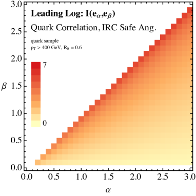
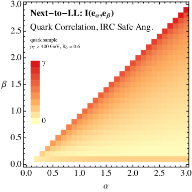
Refer to caption
(a)
Refer to caption
(b)


Refer to caption
(c)
Refer to caption
(d)


Figure 14: Correlation between two IRC safe angularities (eα,eβ)subscript𝑒𝛼subscript𝑒𝛽({e_{\alpha}},{e_{\beta}}) on a pure quark jet sample. Top: the LL and NLL analytic calculations. Bottom: the Pythia 8 and Herwig++ parton showers.
Refer to caption
(a)
Refer to caption
(b)


Refer to caption
(c)
Refer to caption
(d)


Figure 15: Same as Fig. 14, but on a pure gluon sample.

We first study the correlation between IRC safe angularities with different angular exponents, as measured by I(eα;eβ)𝐼subscript𝑒𝛼subscript𝑒𝛽I({e_{\alpha}};{e_{\beta}}). This is shown for a pure sample of quark jets in Fig. 14 and for a pure sample of gluon jets in Fig. 15. Two angularities are highly correlated when their angular exponents are close to one another, and become increasingly uncorrelated as the angular exponents move farther apart. This behavior can be understood from the definition of the angularities. For large values of angular exponent, the angularity is dominated by soft, wide-angle emissions because collinear emissions are suppressed by small angles raised to a high power. By contrast, at small values of the angular exponent, the angularity is dominated by hard collinear emissions. Thus, when two angularities have very different angular exponents, their values are dominated by different physics and so are largely uncorrelated. Unlike the case of the truth overlap in Fig. 5, there is broad agreement between LL, NLL, Pythia 8, and Herwig++ as far as the raw correlations are concerned.
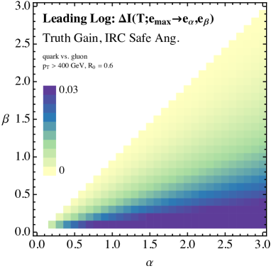
Refer to caption
(a)
Refer to caption
(b)


Refer to caption
(c)
Refer to caption
(d)


Figure 16: Improvement in the truth overlap by using two IRC safe angularities (eα,eβ)subscript𝑒𝛼subscript𝑒𝛽({e_{\alpha}},{e_{\beta}}) as compared to only one, I(T;eα,eβ)max[I(T;eα),I(T;eβ)]𝐼𝑇subscript𝑒𝛼subscript𝑒𝛽𝐼𝑇subscript𝑒𝛼𝐼𝑇subscript𝑒𝛽I(T;e_{\alpha},e_{\beta})-\max[I(T;e_{\alpha}),I(T;e_{\beta})]. Top: the LL and NLL analytic calculations. Bottom: the Pythia 8 and Herwig++ parton showers.

Next, we want to understand better the degree to which two angularities have more truth overlap than one angularity. In Fig. 16, we plot ΔI(T,emaxeα,eβ)\Delta I(T,e_{\rm max}\to{e_{\alpha}},{e_{\beta}}) from Eq. (36), namely the pairwise truth overlap I(T;eα,eβ)𝐼𝑇subscript𝑒𝛼subscript𝑒𝛽I(T;{e_{\alpha}},{e_{\beta}}) minus the truth overlap of the stronger angularity max{I(T;eα),I(T;eβ)}𝐼𝑇subscript𝑒𝛼𝐼𝑇subscript𝑒𝛽\max\{I(T;{e_{\alpha}}),I(T;{e_{\beta}})\}. The information gain is on the order of 10% (𝒪(0.01)𝒪0.01\mathcal{O}(0.01) compared to a baseline truth overlap of 𝒪(0.1)𝒪0.1\mathcal{O}(0.1)). As in Fig. 5, there are quite substantial differences between the various methods. It is interesting that in Pythia 8 one can already achieve considerable gains in performance just off the diagonal, i.e. for observables that are not very different. This may be because when α𝛼\alpha and β𝛽\beta are close (compare to Eq. (29)),

eαeβ(αβ)iziθiαlogθi+,similar-to-or-equalssubscript𝑒𝛼subscript𝑒𝛽𝛼𝛽subscript𝑖subscript𝑧𝑖superscriptsubscript𝜃𝑖𝛼subscript𝜃𝑖{e_{\alpha}}-{e_{\beta}}\simeq(\alpha-\beta)\sum_{i}z_{i}\theta_{i}^{\alpha}\log\theta_{i}+\ldots, (138)

and θiαlogθisuperscriptsubscript𝜃𝑖𝛼subscript𝜃𝑖\theta_{i}^{\alpha}\log\theta_{i} is similar to the optimal kernel found in Refs. Gallicchio:2011xq ; Gallicchio:2012ez .
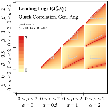
Refer to caption
(a)
Refer to caption
(b)


Refer to caption
(c)
Refer to caption
(d)


Figure 17: Correlation between two generalized angularities (λαρ,λβκ)subscriptsuperscript𝜆𝜌𝛼subscriptsuperscript𝜆𝜅𝛽({\lambda^{\rho}_{\alpha}},{\lambda^{\kappa}_{\beta}}) on a pure quark sample. Top: the LL and NLL analytic calculations. Bottom: the Pythia 8 and Herwig++ parton showers. As in Fig. 13, β{0,0.5,1,2}𝛽00.512\beta\in\{0,0.5,1,2\} and we sweep 0κ20𝜅20\leq\kappa\leq 2.
Refer to caption
(a)
Refer to caption
(b)


Refer to caption
(c)
Refer to caption
(d)


Figure 18: Same as Fig. 17, but for a pure gluon sample.
Refer to caption
(a)
Refer to caption
(b)


Figure 19: Improvement in the truth overlap by using two generalized angularities (λαρ,λβκ)subscriptsuperscript𝜆𝜌𝛼subscriptsuperscript𝜆𝜅𝛽({\lambda^{\rho}_{\alpha}},{\lambda^{\kappa}_{\beta}}) as compared to only one, I(T;λαρ,λβκ)max[I(T;λαρ),I(T;λβκ)]𝐼𝑇subscriptsuperscript𝜆𝜌𝛼subscriptsuperscript𝜆𝜅𝛽𝐼𝑇subscriptsuperscript𝜆𝜌𝛼𝐼𝑇subscriptsuperscript𝜆𝜅𝛽I(T;{\lambda^{\rho}_{\alpha}},{\lambda^{\kappa}_{\beta}})-\max[I(T;{\lambda^{\rho}_{\alpha}}),I(T;{\lambda^{\kappa}_{\beta}})]. We only show the Pythia 8 and Herwig++ parton showers since the LL and NLL analytic calculations are not sufficiently accurate to extract subtle differences in truth overlap.

Turning to the generalized angularities, in Figs. 17 and 18 we show the correlations on pure quark and gluon samples as measured by I(λαρ,λβκ)𝐼subscriptsuperscript𝜆𝜌𝛼subscriptsuperscript𝜆𝜅𝛽I({\lambda^{\rho}_{\alpha}},{\lambda^{\kappa}_{\beta}}). As in the IRC unsafe case, there is broad agreement in the overall degree of correlation, though one has to be mindful of the restricted range of validity of the (N)LL calculations. In Fig. 19, we show the improvement of using two generalized angularities compared to one. The LL and NLL calculations are not shown, since those calculations are not accurate enough to assess small differences. The comparison between Pythia 8 and Herwig++ is similar to the IRC safe case, with Pythia 8 being more optimistic about the gains possible by combining observables.
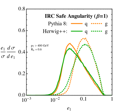
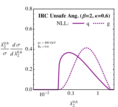
Refer to caption
(a)
Refer to caption
(b)


Refer to caption
(c)
Refer to caption
(d)


Figure 20: Raw distributions of e1subscript𝑒1{e_{1}} (top) and λ20.6subscriptsuperscript𝜆0.62{\lambda^{0.6}_{2}} (bottom) for the NLL calculation (left) and parton showers (right). Note that the NLL distributions lack hadronization corrections that are present in the parton showers, which affects small values of the angularities.
Refer to caption
(a)
Refer to caption
(b)


Figure 21: Double differential distributions in the e1subscript𝑒1{e_{1}}λ20.6subscriptsuperscript𝜆0.62{\lambda^{0.6}_{2}} plane for the NLL calculation (left) and parton showers (right). The contours correspond to the half maximum of d2σ/(dlne1dlnλ20.6)superscriptd2𝜎dsubscript𝑒1dsubscriptsuperscript𝜆0.62\mathrm{d}^{2}\sigma/(\mathrm{d}\ln{e_{1}}\,\mathrm{d}\ln{\lambda^{0.6}_{2}}).

Finally, we show a few raw angularity distributions from the NLL calculation and both parton showers. In Fig. 20, we show single differential distributions for e1subscript𝑒1{e_{1}} as an IRC safe example and λ20.6subscriptsuperscript𝜆0.62{\lambda^{0.6}_{2}} as an IRC unsafe example. Note that the NLL calculations lack important hadronization corrections that are modelled by the parton showers and are particularly important to correctly describe the small angularity region. The NLL result for λ20.6subscriptsuperscript𝜆0.62{\lambda^{0.6}_{2}} cuts off rather sharply at the low end due to our treatment of the QCD Landau pole. The Pythia 8 distributions are more peaked than the Herwig++ distributions, which is part of the reason why Pythia 8 predicts improved discrimination power compared to Herwig++. We then show the double differential distribution for e1subscript𝑒1{e_{1}} and λ20.6subscriptsuperscript𝜆0.62{\lambda^{0.6}_{2}} in Fig. 21, showing only the half-maximum contour for readability. There is an irreducible degree of correlation between these observables due to phase space constraints (see Eq. (60)), but one can see that, while the gluon contours are similar for Pythia 8 and Herwig++, the Pythia 8 contour for quarks is significantly smaller than Herwig++. This explains the enhanced discrimination power predicted by Pythia 8. The NLL contours are much larger in size than either Pythia 8 or Herwig++ because the NLL distributions do not vanish at the phase space boundaries Larkoski:2014tva . The analytic distribution will only vanish at the boundaries starting at NLL order, beyond the accuracy to which double differential cross sections have as-of-yet been computed.

References

  • (1) A. Abdesselam, E. B. Kuutmann, U. Bitenc, G. Brooijmans, J. Butterworth, et al., Boosted objects: A Probe of beyond the Standard Model physics, Eur. Phys. J. C71 (2011) 1661, [arXiv:1012.5412].
  • (2) A. Altheimer, S. Arora, L. Asquith, G. Brooijmans, J. Butterworth, et al., Jet Substructure at the Tevatron and LHC: New results, new tools, new benchmarks, J. Phys. G39 (2012) 063001, [arXiv:1201.0008].
  • (3) A. Altheimer, A. Arce, L. Asquith, J. Backus Mayes, E. Bergeaas Kuutmann, et al., Boosted objects and jet substructure at the LHC, arXiv:1311.2708.
  • (4) J. Gallicchio and M. D. Schwartz, Quark and Gluon Tagging at the LHC, Phys. Rev. Lett. 107 (2011) 172001, [arXiv:1106.3076].
  • (5) J. Gallicchio and M. D. Schwartz, Quark and Gluon Jet Substructure, JHEP 1304 (2013) 090, [arXiv:1211.7038].
  • (6) D. Krohn, M. D. Schwartz, T. Lin, and W. J. Waalewijn, Jet Charge at the LHC, Phys. Rev. Lett. 110 (2013) 212001, [arXiv:1209.2421].
  • (7) CMS Collaboration, S. Chatrchyan et al., Search for a Higgs boson in the decay channel HZZ()qq¯+𝐻𝑍superscript𝑍𝑞¯𝑞superscriptsuperscriptH\to ZZ^{(*)}\to q\bar{q}\ell^{-}\ell^{+} in pp𝑝𝑝pp collisions at s=7𝑠7\sqrt{s}=7 TeV, JHEP 1204 (2012) 036, [arXiv:1202.1416].
  • (8) F. Pandolfi and D. Del Re, Search for the Standard Model Higgs Boson in the HZZllqq𝐻𝑍𝑍𝑙𝑙𝑞𝑞H\to ZZ\to llqq Decay Channel at CMS. PhD thesis, Zurich, ETH, 2012.
  • (9) A. J. Larkoski, G. P. Salam, and J. Thaler, Energy Correlation Functions for Jet Substructure, JHEP 1306 (2013) 108, [arXiv:1305.0007].
  • (10) CMS Collaboration, Performance of quark/gluon discrimination in 8 TeV pp data, Tech. Rep. CMS-PAS-JME-13-002, CERN, Geneva, 2013.
  • (11) CMS Collaboration, Pileup Jet Identification, Tech. Rep. CMS-PAS-JME-13-005, CERN, Geneva, 2013.
  • (12) ATLAS Collaboration, G. Aad et al., Light-quark and gluon jet discrimination in pp collisions at s𝑠\sqrt{s} = 7 TeV with the ATLAS detector, arXiv:1405.6583.
  • (13) ATLAS Collaboration, Performance and Validation of Q-Jets at the ATLAS Detector in pp Collisions at s𝑠\sqrt{s}=8 TeV in 2012, Tech. Rep. ATLAS-CONF-2013-087, 2013.
  • (14) CMS Collaboration, Identifying Hadronically Decaying Vector Bosons Merged into a Single Jet, Tech. Rep. CMS-PAS-JME-13-006, CERN, Geneva, 2013.
  • (15) P. Carruthers and C. Shih, Mutual Information and Forward Backward Correlations in Multi - Hadron Production, Phys. Rev. Lett. 62 (1989) 2073.
  • (16) I. Narsky and F. C. Porter, Statistical analysis techniques in particle physics. Wiley-VCH, Berlin, 2014.
  • (17) H. Casini and M. Huerta, A Finite entanglement entropy and the c-theorem, Phys. Lett. B600 (2004) 142–150, [hep-th/0405111].
  • (18) M. M. Wolf, F. Verstraete, M. B. Hastings, and J. I. Cirac, Area Laws in Quantum Systems: Mutual Information and Correlations, Phys. Rev. Lett. 100 (2008) 070502, [arXiv:0704.3906].
  • (19) P. Calabrese and J. Cardy, Entanglement entropy and conformal field theory, Journal of Physics A Mathematical General 42 (2009) 4005, [arXiv:0905.4013].
  • (20) M. Headrick, Entanglement Renyi entropies in holographic theories, Phys. Rev. D82 (2010) 126010, [arXiv:1006.0047].
  • (21) D. Bertolini, T. Chan, and J. Thaler, Jet Observables Without Jet Algorithms, JHEP 1404 (2014) 013, [arXiv:1310.7584].
  • (22) A. J. Larkoski, D. Neill, and J. Thaler, Jet Shapes with the Broadening Axis, JHEP 1404 (2014) 017, [arXiv:1401.2158].
  • (23) G. Salam Unpublished.
  • (24) S. Catani, G. Turnock, and B. Webber, Jet broadening measures in e+esuperscript𝑒superscript𝑒e^{+}e^{-} annihilation, Phys. Lett. B295 (1992) 269–276.
  • (25) Y. L. Dokshitzer, A. Lucenti, G. Marchesini, and G. Salam, On the QCD analysis of jet broadening, JHEP 9801 (1998) 011, [hep-ph/9801324].
  • (26) A. Banfi, G. P. Salam, and G. Zanderighi, Principles of general final-state resummation and automated implementation, JHEP 0503 (2005) 073, [hep-ph/0407286].
  • (27) A. J. Larkoski and J. Thaler, Aspects of Jets at 100 TeV, arXiv:1406.7011.
  • (28) C. F. Berger, T. Kucs, and G. F. Sterman, Event shape / energy flow correlations, Phys. Rev. D68 (2003) 014012, [hep-ph/0303051].
  • (29) L. G. Almeida, S. J. Lee, G. Perez, G. F. Sterman, I. Sung, et al., Substructure of high-pTsubscript𝑝𝑇p_{T} Jets at the LHC, Phys. Rev. D79 (2009) 074017, [arXiv:0807.0234].
  • (30) S. D. Ellis, C. K. Vermilion, J. R. Walsh, A. Hornig, and C. Lee, Jet Shapes and Jet Algorithms in SCET, JHEP 1011 (2010) 101, [arXiv:1001.0014].
  • (31) P. E. Rakow and B. Webber, Transverse Momentum Moments of Hadron Distributions in QCD Jets, Nucl. Phys. B191 (1981) 63.
  • (32) R. K. Ellis and B. Webber, QCD Jet Broadening in Hadron Hadron Collisions, Conf. Proc. C860623 (1986) 74.
  • (33) E. Farhi, Quantum chromodynamics test for jets, Phys. Rev. Lett. 39 (Dec, 1977) 1587–1588.
  • (34) M. Dasgupta, A. Fregoso, S. Marzani, and G. P. Salam, Towards an understanding of jet substructure, JHEP 1309 (2013) 029, [arXiv:1307.0007].
  • (35) M. Dasgupta, A. Fregoso, S. Marzani, and A. Powling, Jet substructure with analytical methods, Eur. Phys. J. C73 (2013), no. 11 2623, [arXiv:1307.0013].
  • (36) A. J. Larkoski, S. Marzani, G. Soyez, and J. Thaler, Soft Drop, JHEP 1405 (2014) 146, [arXiv:1402.2657].
  • (37) A. Hornig, C. Lee, and G. Ovanesyan, Effective Predictions of Event Shapes: Factorized, Resummed, and Gapped Angularity Distributions, JHEP 0905 (2009) 122, [arXiv:0901.3780].
  • (38) W. J. Waalewijn, Calculating the Charge of a Jet, Phys. Rev. D86 (2012) 094030, [arXiv:1209.3019].
  • (39) H.-M. Chang, M. Procura, J. Thaler, and W. J. Waalewijn, Calculating Track-Based Observables for the LHC, Phys. Rev. Lett. 111 (2013) 102002, [arXiv:1303.6637].
  • (40) H.-M. Chang, M. Procura, J. Thaler, and W. J. Waalewijn, Calculating Track Thrust with Track Functions, Phys. Rev. D88 (2013) 034030, [arXiv:1306.6630].
  • (41) A. Banfi, G. P. Salam, and G. Zanderighi, Infrared safe definition of jet flavor, Eur. Phys. J. C47 (2006) 113–124, [hep-ph/0601139].
  • (42) I. W. Stewart, F. J. Tackmann, and W. J. Waalewijn, Dissecting Soft Radiation with Factorization, arXiv:1405.6722.
  • (43) J. Gallicchio and M. D. Schwartz, Pure Samples of Quark and Gluon Jets at the LHC, JHEP 1110 (2011) 103, [arXiv:1104.1175].
  • (44) M. A. Nielsen and I. L. Chuang, Quantum Computation and Quantum Information. Cambridge University Press, 2000.
  • (45) T. Sjostrand, S. Mrenna, and P. Z. Skands, PYTHIA 6.4 Physics and Manual, JHEP 0605 (2006) 026, [hep-ph/0603175].
  • (46) T. Sjostrand, S. Mrenna, and P. Z. Skands, A Brief Introduction to PYTHIA 8.1, Comput. Phys. Commun. 178 (2008) 852–867, [arXiv:0710.3820].
  • (47) M. Bahr, S. Gieseke, M. Gigg, D. Grellscheid, K. Hamilton, et al., Herwig++ Physics and Manual, Eur. Phys. J. C58 (2008) 639–707, [arXiv:0803.0883].
  • (48) S. Gieseke, D. Grellscheid, K. Hamilton, A. Papaefstathiou, S. Platzer, et al., Herwig++ 2.5 Release Note, arXiv:1102.1672.
  • (49) I. W. Stewart, F. J. Tackmann, and W. J. Waalewijn, N-Jettiness: An Inclusive Event Shape to Veto Jets, Phys. Rev. Lett. 105 (2010) 092002, [arXiv:1004.2489].
  • (50) J. Thaler and K. Van Tilburg, Identifying Boosted Objects with N-subjettiness, JHEP 1103 (2011) 015, [arXiv:1011.2268].
  • (51) J. Thaler and K. Van Tilburg, Maximizing Boosted Top Identification by Minimizing N-subjettiness, JHEP 1202 (2012) 093, [arXiv:1108.2701].
  • (52) M. Cacciari, G. P. Salam, and G. Soyez, FastJet User Manual, Eur. Phys. J. C 72 (2012) 1896, [arXiv:1111.6097].
  • (53) A. J. Larkoski and J. Thaler, Unsafe but Calculable: Ratios of Angularities in Perturbative QCD, JHEP 1309 (2013) 137, [arXiv:1307.1699].
  • (54) A. J. Larkoski, I. Moult, and D. Neill, Toward Multi-Differential Cross Sections: Measuring Two Angularities on a Single Jet, arXiv:1401.4458.
  • (55) C. W. Bauer, S. Fleming, and M. E. Luke, Summing Sudakov logarithms in BXsγ𝐵subscript𝑋𝑠𝛾B\to X_{s}\gamma in effective field theory, Phys. Rev. D63 (2000) 014006, [hep-ph/0005275].
  • (56) C. W. Bauer, S. Fleming, D. Pirjol, and I. W. Stewart, An effective field theory for collinear and soft gluons: heavy to light decays, Phys. Rev. D63 (2001) 114020, [hep-ph/0011336].
  • (57) C. W. Bauer and I. W. Stewart, Invariant operators in collinear effective theory, Phys. Lett. B516 (2001) 134–142, [hep-ph/0107001].
  • (58) C. W. Bauer, D. Pirjol, and I. W. Stewart, Soft collinear factorization in effective field theory, Phys. Rev. D65 (2002) 054022, [hep-ph/0109045].
  • (59) D. E. Soper and M. Spannowsky, Finding physics signals with shower deconstruction, Phys. Rev. D84 (2011) 074002, [arXiv:1102.3480].
  • (60) A. Capella, I. Dremin, J. Gary, V. Nechitailo, and J. Tran Thanh Van, Evolution of average multiplicities of quark and gluon jets, Phys. Rev. D61 (2000) 074009, [hep-ph/9910226].
  • (61) P. Bolzoni, B. Kniehl, and A. Kotikov, Gluon and quark jet multiplicities at N3LO+NNLL, Phys. Rev. Lett. 109 (2012) 242002, [arXiv:1209.5914].
  • (62) M. Procura and I. W. Stewart, Quark Fragmentation within an Identified Jet, Phys. Rev. D81 (2010) 074009, [arXiv:0911.4980].
  • (63) A. Jain, M. Procura, and W. J. Waalewijn, Parton Fragmentation within an Identified Jet at NNLL, JHEP 1105 (2011) 035, [arXiv:1101.4953].
  • (64) V. Gribov and L. Lipatov, Deep inelastic e p scattering in perturbation theory, Sov. J. Nucl. Phys. 15 (1972) 438–450.
  • (65) H. Georgi and H. D. Politzer, Electroproduction scaling in an asymptotically free theory of strong interactions, Phys. Rev. D9 (1974) 416–420.
  • (66) D. Gross and F. Wilczek, Asymptotically Free Gauge Theories. II, Phys. Rev. D9 (1974) 980–993.
  • (67) G. Altarelli and G. Parisi, Asymptotic Freedom in Parton Language, Nucl. Phys. B126 (1977) 298.
  • (68) Y. L. Dokshitzer, Calculation of the Structure Functions for Deep Inelastic Scattering and e+esuperscript𝑒superscript𝑒e^{+}e^{-} Annihilation by Perturbation Theory in Quantum Chromodynamics., Sov. Phys. JETP 46 (1977) 641–653.
  • (69) M. Dasgupta and G. Salam, Resummation of nonglobal QCD observables, Phys. Lett. B512 (2001) 323–330, [hep-ph/0104277].
  • (70) S. Catani, B. Webber, and G. Marchesini, QCD coherent branching and semiinclusive processes at large x, Nucl. Phys. B349 (1991) 635–654.
  • (71) J. M. Butterworth, A. R. Davison, M. Rubin, and G. P. Salam, Jet substructure as a new Higgs search channel at the LHC, Phys. Rev. Lett. 100 (2008) 242001, [arXiv:0802.2470].
  • (72) M. Procura, W. J. Waalewijn, and L. Zeune, Resummation of Double-Differential Cross Sections and Fully-Unintegrated Parton Distribution Functions, arXiv:1410.6483.
  • (73) T. Becher and M. D. Schwartz, A precise determination of αssubscript𝛼𝑠\alpha_{s} from LEP thrust data using effective field theory, JHEP 0807 (2008) 034, [arXiv:0803.0342].
  • (74) L. G. Almeida, S. D. Ellis, C. Lee, G. Sterman, I. Sung, et al., Comparing and counting logs in direct and effective methods of QCD resummation, JHEP 1404 (2014) 174, [arXiv:1401.4460].