PRECISE ATMOSPHERIC PARAMETERS FOR THE SHORTEST PERIOD BINARY WHITE DWARFS: GRAVITATIONAL WAVES, METALS, AND PULSATIONS*

Abstract

We present a detailed spectroscopic analysis of 61 low mass white dwarfs and provide precise atmospheric parameters, masses, and updated binary system parameters based on our new model atmosphere grids and the most recent evolutionary model calculations. For the first time, we measure systematic abundances of He, Ca and Mg for metal-rich extremely low mass white dwarfs and examine the distribution of these abundances as a function of effective temperature and mass. Based on our preliminary results, we discuss the possibility that shell flashes may be responsible for the presence of the observed He and metals. We compare stellar radii derived from our spectroscopic analysis to model-independent measurements and find good agreement except for those white dwarfs with $T_{\rm eff}$ $\lesssim$ 10,000 K. We also calculate the expected gravitational wave strain for each system and discuss their significance to the $eLISA$ space-borne gravitational wave observatory. Finally, we provide an update on the instability strip of extremely low mass white dwarf pulsators.

1. INTRODUCTION

Extremely low mass (ELM) white dwarfs (WDs) with surface gravities of $\log g$ $\lesssim$ 7.0 (or masses $M$ $\lesssim$ 0.30 $M_{\odot}$) are presumed to have He cores and are necessarily the product of the evolution of compact binary systems. The Universe is not yet old enough to have produced such ELM WDs through normal single-star evolution (Marsh et al. 1995). These extreme products of binary evolution represent the possible progenitors of type Ia supernovae (Iben & Tutukov 1984), underluminous .Ia supernovae (Bildsten et al. 2007), AM CVn systems (Breedt et al. 2012; Kilic et al. 2014b) and possibly even R CrB stars (Webbink 1984; Clayton 2013).

One of the first spectroscopically confirmed ELM WDs was found as the companion to the millisecond pulsar PSR J1012+5307 (van Kerkwijk et al. 1996; Callanan et al. 1998). Several more ELM WDs have been spectroscopically identified as pulsar companions (e.g. Antoniadis et al. 2013; Kaplan et al. 2013, 2014a; Ransom et al. 2014; Smedley et al. 2014, and references therein) and in other short period binary systems (Heber et al. 2003; Liebert et al. 2004; Kawka et al. 2006; Mullally et al. 2009; Kulkarni & van Kerkwijk 2010; Marsh et al. 2011; Vennes et al. 2011; Silvotti et al. 2012).

Based on a comparison of the mass distribution of post-common envelope binaries and wide WD+main sequence binaries from the Sloan Digital Sky Survey (SDSS), Rebassa-Mansergas et al. (2011) confirmed that the majority of low-mass WDs reside in close binary systems (Marsh et al. 1995). Furthermore, the EL CVn-type binaries, with orbital periods $P_{\rm orb}$ $\approx$ 0.7–2.2 d, published in Maxted et al. (2013) and Maxted et al. (2014) also represent potential progenitors to ELM WDs.

Existing in such tight binary systems, we expect ELM WDs to be sources of gravitational waves (Hermes et al. 2012c; Kilic et al. 2013a) as their orbits decay due to the loss of orbital angular momentum. Hence, they represent potential testbeds for general relativity and the shortest period systems serve as verification sources for future gravitational wave detectors such as $eLISA$ (Amaro-Seoane et al. 2013). The close nature of these systems also gives rise to phenomena such as ellipsoidal variations due to tidal distortions and Doppler beaming. Both of these phenomena manifest themselves in the light curves of ELM WDs. The analysis of ellipsoidal variations (Hermes et al. 2012a; Gianninas et al. 2014), as well as parallax measurements (Kilic et al. 2013b) and eclipse modeling (Hermes et al. 2012c; Kaplan et al. 2014b; Bours et al. 2014), provide model-independent methods for measuring the stellar radius. Recent studies (Kilic et al. 2013b; Kaplan et al. 2014b; Gianninas et al. 2014) have brought to light a discrepancy between the radii inferred from spectroscopic analyses to those measured by model-independent methods for the coolest ELM WDs. Precise measurements of the atmospheric parameters of ELM WDs are needed in order to shed light on this issue.

The ELM Survey (Brown et al. 2010, 2012, 2013; Kilic et al. 2010, 2011, 2012) has been searching for short-period ($P_{\rm orb}\leqslant$ 1 day) ELM WD binaries for several years now with considerable success. Candidates are selected mostly using available SDSS photometry and then followed-up with optical time-series spectroscopy through which radial velocity (RV) variations are detected. In some cases, SDSS spectroscopy has also been useful in identifying potential ELM WD candidates. So far, over 60 ELM WD binaries have been discovered by the ELM Survey and over 30 of them will merge within a Hubble time (Brown et al. 2013).

All of the previously published ELM Survey analyses have noted the presence of the Ca ii $\lambda$3934 K resonance line in the spectra of all ELM WDs with $\log g$ $\leqslant$ 6.0. The fact that all of the lowest mass ELM WDs share this spectroscopic signature suggests that a physical phenomenon related to their evolution might be responsible. However, a systematic study of the metal abundances in ELM WDs has never been performed; abundances have only been measured for a handful of systems. These include the hot ELM WD GALEX J1717+6757 (Vennes et al. 2011; Hermes et al. 2014a), the WD companion to PSR J1816+4510 (Kaplan et al. 2013), and, most recently, Gianninas et al. (2014) analyzed the unusually metal-rich and tidally distorted ELM WD binary J0745+1949 (hereafter, J0745).

For canonical mass WDs, Zuckerman et al. (2003, 2010) showed that $\approx$ 25% of hydrogen atmosphere DA WDs and $\approx$ 30% of helium atmosphere DB WDs are polluted with metals based on a detailed analysis of high resolution spectroscopy. The more recent analysis of Koester et al. (2014) suggests that the number of metal-rich WDs is closer to 60%. For WDs with $T_{\rm eff}$ $\leq$ 20,000 K, this phenomenon is understood to be the consequence of ongoing accretion from a circumstellar disk resulting from the tidal disruption of a rocky body venturing too close to the host WD. This has been confirmed through the detection of infrared (IR) excesses due to the emission of a dusty (e.g. Jura 2003; Kilic et al. 2006; Farihi et al. 2009; Barber et al. 2012) or gaseous (e.g. Melis et al. 2012; Gänsicke et al. 2006; Gänsicke 2011, and references therein) debris disk surrounding the WD. To date, there is no evidence that analogous disks are present around polluted ELM WD binaries.

Kaplan et al. (2013) suggested that the observed metals could be the result of a recent shell flash that would serve to mix the outer layers of the WD and bring metals to the surface. The evolutionary models of Althaus et al. (2013) certainly suggest that ELM WDs with masses between 0.18 $M_{\odot}$ and 0.36 $M_{\odot}$ undergo a series of H-shell flashes as they evolve. However, this would not explain the presence of Ca for ELM WDs with masses $<$ 0.18 $M_{\odot}$, where shell flashes are not predicted.

In this paper, we present a comprehensive and homogeneous spectroscopic analysis of the entire ELM Survey sample including updated measurements of the atmospheric parameters, $T_{\rm eff}$ and $\log g$, as well as abundances of all the observed metals. We also provide improved mass estimates for both components of the system and use these to calculate the expected gravitational wave strain of the system. Furthermore, this is the first time we have a large enough sample of ELM WDs with independent radius measurements to explore the discrepancies with spectroscopically derived radii. We summarize, in Section 2, the current sample of WDs from the ELM Survey and briefly describe our observations. Section 3 lists and explains the various grids of model atmospheres used in our study. In Section 4, we present the results of our analysis including our updated physical and binary parameters. Section 5 discusses the ensemble properties of our sample. Finally, Section 6 outlines our conclusions and we comment on future avenues of research.

2. ELM SURVEY SAMPLE

The sample that we analyze includes a total of 61 ELM WD binaries from the ELM Survey. The bulk of this sample is comprised of the 58 ELM WDs listed in Table 3 of Brown et al. (2013) but also includes three additional ELM WDs which have been published in separate papers since then. These three ELM WDs are the metal-rich and tidally distorted ELM WD J0745 (Gianninas et al. 2014) and the two pulsating ELM WDs J1614+1912 and J2228+3623 (Hermes et al. 2013b). Of these 61 ELM WDs, 55 are confirmed as being in short-period binary systems through the detection of RV variability and their orbital periods ($P$) and velocity semi-amplitudes ($K$) are well constrained. The six remaining ELM WDs (J0900+0234, J1448+1342, J1614+1912, J2228+3623, J2252$-$0056, J2345$-$0102) do not display significant radial velocity variability and only upper limits for $K$ have been measured.

The spectra of these 61 ELM WDs were obtained using five distinct setups on two different telescopes. A total of 57 targets were observed at the 6.5m MMT telescope with the Blue Channel spectrograph (Schmidt et al. 1989). With only one exception, the observations were obtained using the 832 line mm^-1 grating but with two different slit widths. First, 35 targets were observed using a 1$\farcs$0 slit providing a spectral resolution of 1.0 Å and an additional 21 targets were observed using a 1$\farcs$25 slit achieving a spectral resolution of 1.2 Å. Finally, the spectra of J0651+2844 (hereafter, J0651) were obtained using the 800 line mm^-1 grating coupled with a 1$\farcs$0 slit producing a resolution of 2.3 Å. All the spectra obtained at the MMT provide spectral coverage from 3600 Å to 4500 Å spanning the Balmer series from H$\gamma$ to the Balmer jump.

The four remaining targets were observed using the Fred Lawrence Whipple Observatory’s (FLWO) 1.5m Tilinghast telescope equipped with the FAST spectrograph (Fabricant et al. 1998) and the 600 line mm^-1 grating. Three targets were observed with a 2$\farcs$0 slit providing a resolution of 2.3 Å with the remaining target having been observed through a 1$\farcs$5 slit for a resolution of 1.7 Å. The observations obtained at FLWO provide a slightly better spectral coverage than the MMT observations, covering from 3500 Å to 5500 Å and thus include H$\beta$ as well.

We note that the nature of the ELM Survey and the necessity of obtaining multiple observations for each ELM WD system to confirm its RV variability and, subsequently, to sample the full binary orbit, provides high signal-to-noise ratio (S/N) observations for the majority of the ELM WDs in our sample with the exception of the very faintest targets. High S/N observations are crucial if we hope to accurately and precisely determine the atmospheric parameters of ELM WDs (see Section 3 and Fig. 12 of Gianninas et al. 2005, for a demonstration of the importance of S/N in the determination of $T_{\rm eff}$ and $\log g$).

Finally, the excellent data quality has also allowed us to easily discern the presence of Ca, as well as Mg, in the atmosphere of many of these ELM WDs. There have been cases where observed Ca lines have been identified as being interstellar in origin. Notably, Silvotti et al. (2012), who analyzed the sdB+WD system KIC 6614501, and Kaplan et al. (2014a), in their study of one of the WD companions to PSR J0337+1715, concluded that the Ca lines they observed in the WD spectrum were interstellar in origin. This conclusion was reached by observing that the Ca lines were not Doppler-shifted along with the Balmer lines. In the ELM Survey sample, the individual spectra used for the RV measurements tend to show both a stationary interstellar component and a photospheric component whose RV correlates with that of the Balmer lines. In all cases, the photospheric component dominates but only a few WDs have enough spectra obtained at quadrature, and at a high enough S/N, to even attempt to separate the two components. We therefore caution that our Ca abundances should be considered as upper limits.

3. MODEL ATMOSPHERES

3.1. Pure Hydrogen Model Atmospheres

For the analysis of the hydrogen Balmer lines, we use hydrogen-rich model atmospheres and synthetic spectra that are derived from the model atmosphere code originally described in Bergeron et al. (1995) and references therein, with recent improvements discussed in Tremblay & Bergeron (2009). Briefly, our models assume a plane-parallel geometry, hydrostatic equilibrium and local thermodynamic equilibrium (LTE). The assumption of LTE is justified as our model grid is restricted to $T_{\rm eff}$ $\leqslant$ 35,000 K where NLTE effects are not yet significant, even for $\log g$ $<$ 7.0 (Napiwotzki 1997). Furthermore, our models adopt the ML2/$\alpha$ = 0.8 parametrization of the mixing length theory as prescribed by Tremblay et al. (2010). Finally, we utilize the new Stark broadening profiles from Tremblay & Bergeron (2009) that include the occupation probability formalism of Hummer & Mihalas (1988) directly in the line profile calculation. For the purposes of fitting the spectra of our ELM WD sample, we have computed a new model grid which we have extended to much lower surface gravities. Our full model grid covers $T_{\rm eff}$ from 4000 K to 35,000 K in steps ranging from 250 to 5000 K, and $\log g$ from 4.5 to 9.5 in steps of 0.25 dex.

3.2. Mixed Hydrogen/Helium Model Atmospheres

For the five ELM WDs which contain helium lines in their optical spectra, we have computed a separate grid of models. This distinct model grid covers $T_{\rm eff}$ from 4500 K to 30,000 K in steps ranging from 250 to 5000 K, $\log g$ from 4.75 to 8.0 in steps of 0.25 dex and $\log$ (He/H) from $-$4.0 to 0.0 in steps of 1.0 dex. These models are identical to the pure hydrogen models but also include helium which is treated according to the formalism presented in Bergeron et al. (2011), including the improved Stark broadening profiles from Beauchamp et al. (1997) for over 20 lines of neutral helium. These line profiles are similar to those presented in Beauchamp et al. (1996) with the exception that at low temperatures ($T_{\rm eff}$ $<$ 10,800 K) the free-free absorption coefficient of the negative helium ion of John (1994) is now used.

3.3. Model Atmospheres with Metals

To measure the abundances of Mg & Ca based on their observed absorption lines, we computed separate grids of model atmospheres and synthetic spectra. We performed these calculations using the same code that was used to model the heavily metal polluted DBZ star J0738+1835 (Dufour et al. 2012) and the metal-rich ELM WD J0745 (Gianninas et al. 2014). Keeping $T_{\rm eff}$ ad $\log g$ fixed at the values determined from the Balmer line fits of each metal-rich ELM WD, we proceed to calculate several grids of synthetic spectra, one for each element of interest (i.e. Mg & Ca). The individual grids cover a range of abundances from $\log[n({\rm Z})/n({\rm H})]$ = $-$3.0 to $-$10.0, in steps of 0.5 dex.

Model fits (red) to the individual Balmer line profiles (black) for 55 WDs from the ELM Survey. The lines range from H$\gamma$ (bottom) to H12 (top), each offset by a factor of 0.2 for clarity. The best-fit values of $T_{\rm eff}$ and $\log g$ are indicated at the bottom of each panel.

(Continued)

(Continued)

(Continued)

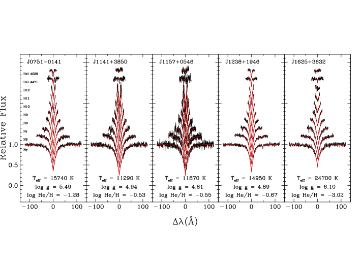
Figure -2.— Model fits (red) to the hydrogen Balmer line, and the He i $\lambda$4471 and He i $\lambda$4026 lines in the observed optical spectra (black) of five ELM WDs. The lines range from H$\gamma$ (bottom) to H12 in addition to He i $\lambda$4471 and He i $\lambda$4026 (top), each offset by a factor of 0.2 for clarity. The best-fit values of $T_{\rm eff}$, $\log g$, and $\log$ (He/H) are indicated at the bottom of each panel.

4. SPECTROSCOPIC ANALYSIS

4.1. Spectroscopic Fits

Our Balmer line fits use the so-called spectroscopic technique developed by Bergeron et al. (1992) and described at length in Gianninas et al. (2011) and references therein. Briefly, we first normalize each individual Balmer line to a continuum set to unity, in both the observed and model spectra. The comparison with the synthetic spectra, which are convolved with an appropriate Gaussian instrumental profile (1.0, 1.7, 2.0, 2.3 Å), is then carried out in terms of these normalized line shapes only. Next, we use our grid of model spectra to determine $T_{\rm eff}$ and $\log g$ using a minimization technique which relies on the nonlinear least-squares method of Levenberg-Marquardt (Press et al. 1986), which is based on a steepest descent method. One important difference between our procedure and that of Gianninas et al. (2011) is that we fit higher-order Balmer lines up to and including H12. These higher-order Balmer lines are still present in low surface gravity ELM WDs and provide additional constraints on our measurement of $\log g$. Furthermore, to ensure the homogeneity of our analysis, we do not fit H$\beta$ for the four objects whose spectra were obtained at FLWO. We have compared the $T_{\rm eff}$ and $\log g$ values from fits with and without H$\beta$ and the results agree within the uncertainties. Consequently, we fit only the lines from H$\gamma$ to H12 for our entire sample. For the ELM WDs whose optical spectra also contain lines due to Ca or Mg, we exclude the affected wavelength ranges from both the normalization and fitting routines.

Table 1ELM WD Physical Parameters

SDSS	$T_{\rm eff}$		$\log g$		Mass	Radius		$g_{0}$		$M_{g}$		$d$		$\tau_{\rm cool}$
	(K)		(cm s-2)		($M_{\odot}$)	($R_{\odot}$)		(mag)		(mag)		(kpc)		(Gyr)
J0022+0031	20460 $\pm$	310	7.58 $\pm$	0.04	0.457	0.0182 $\pm$	0.0013	19.284 $\pm$	0.033	9.84 $\pm$	0.19	0.775 $\pm$	0.068	0.215 $\pm$	0.129
J0022$-$1014	20730 $\pm$	340	7.28 $\pm$	0.05	0.375	0.0233 $\pm$	0.0019	19.581 $\pm$	0.031	9.28 $\pm$	0.21	1.151 $\pm$	0.113	0.042 $\pm$	0.021
J0056$-$0611	12230 $\pm$	180	6.17 $\pm$	0.04	0.174	0.0565 $\pm$	0.0061	17.208 $\pm$	0.023	8.37 $\pm$	0.27	0.586 $\pm$	0.073	0.959 $\pm$	0.081
J0106$-$1000	16970 $\pm$	260	6.10 $\pm$	0.05	0.191	0.0642 $\pm$	0.0068	19.595 $\pm$	0.023	7.45 $\pm$	0.26	2.690 $\pm$	0.323	0.497 $\pm$	0.168
J0112+1835	10020 $\pm$	140	5.76 $\pm$	0.05	0.161	0.0874 $\pm$	0.0108	17.110 $\pm$	0.016	7.89 $\pm$	0.31	0.697 $\pm$	0.100	1.661 $\pm$	0.169
J0152+0749	10840 $\pm$	180	5.92 $\pm$	0.05	0.168	0.0748 $\pm$	0.0084	18.033 $\pm$	0.009	8.03 $\pm$	0.29	1.001 $\pm$	0.134	1.384 $\pm$	0.130
J0345+1748	8680 $\pm$	120	6.83 $\pm$	0.04	0.220	0.0297 $\pm$	0.0028	16.500 $\pm$	0.300	10.84 $\pm$	0.27	0.134 $\pm$	0.025	1.020 $\pm$	0.094
J0651+2844	16340 $\pm$	260	6.81 $\pm$	0.05	0.252	0.0325 $\pm$	0.0031	19.111 $\pm$	0.012	9.00 $\pm$	0.24	1.053 $\pm$	0.116	0.183 $\pm$	0.110
J0730+1703	12030 $\pm$	220	6.30 $\pm$	0.05	0.183	0.0503 $\pm$	0.0058	20.076 $\pm$	0.028	8.66 $\pm$	0.29	1.921 $\pm$	0.261	1.003 $\pm$	0.159
J0745+1949	8380 $\pm$	130	6.21 $\pm$	0.07	0.164	0.0526 $\pm$	0.0076	16.491 $\pm$	0.008	9.75 $\pm$	0.39	0.223 $\pm$	0.040	4.232 $\pm$	0.593
J0751$-$0141	15740 $\pm$	250	5.49 $\pm$	0.05	0.194	0.1315 $\pm$	0.0104	17.490 $\pm$	0.015	6.03 $\pm$	0.19	1.958 $\pm$	0.168	0.258 $\pm$	0.141
J0755+4800	19520 $\pm$	300	7.42 $\pm$	0.05	0.409	0.0207 $\pm$	0.0016	16.039 $\pm$	0.017	9.64 $\pm$	0.20	0.190 $\pm$	0.017	0.096 $\pm$	0.008
J0755+4906	13590 $\pm$	280	6.13 $\pm$	0.06	0.176	0.0597 $\pm$	0.0077	20.242 $\pm$	0.023	8.03 $\pm$	0.33	2.768 $\pm$	0.417	0.803 $\pm$	0.115
J0802$-$0955	16980 $\pm$	270	6.44 $\pm$	0.05	0.208	0.0452 $\pm$	0.0047	18.885 $\pm$	0.012	8.21 $\pm$	0.26	1.366 $\pm$	0.161	0.356 $\pm$	0.160
J0811+0225	13540 $\pm$	200	5.67 $\pm$	0.04	0.181	0.1035 $\pm$	0.0111	18.669 $\pm$	0.024	6.84 $\pm$	0.26	2.321 $\pm$	0.284	0.485 $\pm$	0.071
J0815+2309	21430 $\pm$	330	5.84 $\pm$	0.05	0.207	0.0903 $\pm$	0.0092	17.805 $\pm$	0.015	6.27 $\pm$	0.25	2.025 $\pm$	0.234	0.380 $\pm$	0.197
J0818+3536	10360 $\pm$	190	5.86 $\pm$	0.09	0.165	0.0790 $\pm$	0.0128	20.756 $\pm$	0.026	8.03 $\pm$	0.40	3.512 $\pm$	0.659	1.613 $\pm$	0.183
J0822+2753	8980 $\pm$	130	6.65 $\pm$	0.05	0.188	0.0340 $\pm$	0.0037	18.314 $\pm$	0.013	10.42 $\pm$	0.30	0.380 $\pm$	0.053	1.129 $\pm$	0.169
J0825+1152	27180 $\pm$	400	6.60 $\pm$	0.04	0.287	0.0443 $\pm$	0.0038	18.774 $\pm$	0.018	7.34 $\pm$	0.22	1.938 $\pm$	0.198	0.083 $\pm$	0.089
J0840+1527	13670 $\pm$	230	5.04 $\pm$	0.05	0.192	0.2198 $\pm$	0.0241	19.319 $\pm$	0.027	5.19 $\pm$	0.27	6.711 $\pm$	0.846	0.181 $\pm$	0.030
J0845+1624	19620 $\pm$	310	7.51 $\pm$	0.05	0.434	0.0191 $\pm$	0.0015	19.817 $\pm$	0.020	9.81 $\pm$	0.20	1.003 $\pm$	0.093	0.130 $\pm$	0.056
J0849+0445	10290 $\pm$	150	6.29 $\pm$	0.05	0.178	0.0499 $\pm$	0.0060	19.292 $\pm$	0.020	9.05 $\pm$	0.30	1.119 $\pm$	0.156	1.617 $\pm$	0.150
J0900+0234	8490 $\pm$	130	6.26 $\pm$	0.07	0.167	0.0502 $\pm$	0.0071	18.142 $\pm$	0.016	9.79 $\pm$	0.38	0.467 $\pm$	0.082	4.188 $\pm$	0.660
J0917+4638	12240 $\pm$	180	5.75 $\pm$	0.04	0.174	0.0918 $\pm$	0.0099	18.764 $\pm$	0.019	7.31 $\pm$	0.27	1.956 $\pm$	0.242	0.792 $\pm$	0.095
J0923+3028	18500 $\pm$	290	6.88 $\pm$	0.05	0.279	0.0316 $\pm$	0.0028	15.709 $\pm$	0.019	8.83 $\pm$	0.23	0.238 $\pm$	0.025	0.079 $\pm$	0.075
J1005+0542	16590 $\pm$	260	7.38 $\pm$	0.05	0.388	0.0210 $\pm$	0.0017	19.763 $\pm$	0.023	9.93 $\pm$	0.20	0.927 $\pm$	0.087	0.166 $\pm$	0.025
J1005+3550	10060 $\pm$	140	6.02 $\pm$	0.05	0.168	0.0665 $\pm$	0.0078	19.004 $\pm$	0.610	8.48 $\pm$	0.30	1.273 $\pm$	0.402	1.861 $\pm$	0.115
J1046$-$0153	14860 $\pm$	230	7.37 $\pm$	0.05	0.375	0.0210 $\pm$	0.0017	18.098 $\pm$	0.018	10.13 $\pm$	0.20	0.392 $\pm$	0.037	0.223 $\pm$	0.038
J1053+5200	16370 $\pm$	240	6.54 $\pm$	0.04	0.213	0.0409 $\pm$	0.0040	18.953 $\pm$	0.020	8.50 $\pm$	0.24	1.234 $\pm$	0.138	0.353 $\pm$	0.152
J1056+6536	21010 $\pm$	360	7.10 $\pm$	0.05	0.338	0.0272 $\pm$	0.0024	19.784 $\pm$	0.023	8.92 $\pm$	0.22	1.489 $\pm$	0.153	0.009 $\pm$	0.036
J1104+0918	16700 $\pm$	260	7.61 $\pm$	0.05	0.454	0.0174 $\pm$	0.0013	16.659 $\pm$	0.016	10.32 $\pm$	0.19	0.186 $\pm$	0.017	0.267 $\pm$	0.178
J1112+1117	9560 $\pm$	140	6.30 $\pm$	0.06	0.177	0.0490 $\pm$	0.0061	16.307 $\pm$	0.016	9.33 $\pm$	0.33	0.248 $\pm$	0.038	2.428 $\pm$	0.347
J1141+3850	11290 $\pm$	210	4.94 $\pm$	0.10	0.177	0.2358 $\pm$	0.0392	19.058 $\pm$	0.017	5.42 $\pm$	0.39	5.330 $\pm$	0.967	0.233 $\pm$	0.074
J1151+5858	15430 $\pm$	300	6.10 $\pm$	0.06	0.183	0.0632 $\pm$	0.0077	20.150 $\pm$	0.025	7.66 $\pm$	0.30	3.150 $\pm$	0.441	0.649 $\pm$	0.149
J1157+0546	11870 $\pm$	260	4.81 $\pm$	0.14	0.186	0.2798 $\pm$	0.0575	19.818 $\pm$	0.024	4.94 $\pm$	0.49	9.432 $\pm$	2.140	0.152 $\pm$	0.056
J1233+1602	11700 $\pm$	240	5.59 $\pm$	0.07	0.169	0.1092 $\pm$	0.0148	19.911 $\pm$	0.017	7.03 $\pm$	0.34	3.777 $\pm$	0.599	0.781 $\pm$	0.108
J1234$-$0228	17800 $\pm$	260	6.61 $\pm$	0.04	0.229	0.0391 $\pm$	0.0037	17.855 $\pm$	0.016	8.43 $\pm$	0.23	0.766 $\pm$	0.082	0.285 $\pm$	0.142
J1238+1946	14950 $\pm$	240	4.89 $\pm$	0.05	0.210	0.2716 $\pm$	0.0226	17.291 $\pm$	0.023	4.55 $\pm$	0.19	3.529 $\pm$	0.319	0.104 $\pm$	0.029
J1422+4352	12770 $\pm$	250	6.11 $\pm$	0.06	0.174	0.0606 $\pm$	0.0077	19.822 $\pm$	0.023	8.12 $\pm$	0.32	2.187 $\pm$	0.323	0.875 $\pm$	0.102
J1436+5010	17370 $\pm$	250	6.66 $\pm$	0.04	0.233	0.0375 $\pm$	0.0035	18.236 $\pm$	0.015	8.58 $\pm$	0.23	0.855 $\pm$	0.091	0.247 $\pm$	0.146
J1439+1002	14520 $\pm$	220	6.36 $\pm$	0.05	0.185	0.0471 $\pm$	0.0050	17.938 $\pm$	0.012	8.42 $\pm$	0.26	0.803 $\pm$	0.098	0.544 $\pm$	0.161
J1443+1509	9170 $\pm$	130	6.71 $\pm$	0.06	0.200	0.0328 $\pm$	0.0038	18.650 $\pm$	0.016	10.41 $\pm$	0.32	0.445 $\pm$	0.065	0.977 $\pm$	0.125
J1448+1342	12300 $\pm$	360	6.99 $\pm$	0.06	0.269	0.0274 $\pm$	0.0028	19.286 $\pm$	0.023	9.94 $\pm$	0.29	0.738 $\pm$	0.098	0.336 $\pm$	0.089
J1512+2615	11380 $\pm$	180	6.93 $\pm$	0.06	0.251	0.0284 $\pm$	0.0031	19.474 $\pm$	0.019	10.03 $\pm$	0.27	0.774 $\pm$	0.097	0.389 $\pm$	0.074
J1518+0658	9940 $\pm$	140	6.82 $\pm$	0.04	0.224	0.0306 $\pm$	0.0030	17.581 $\pm$	0.017	10.24 $\pm$	0.27	0.293 $\pm$	0.036	0.714 $\pm$	0.053
J1538+0252	10260 $\pm$	150	5.98 $\pm$	0.06	0.168	0.0694 $\pm$	0.0093	18.721 $\pm$	0.014	8.33 $\pm$	0.33	1.195 $\pm$	0.183	1.726 $\pm$	0.106
J1557+2823	12560 $\pm$	190	7.76 $\pm$	0.05	0.461	0.0147 $\pm$	0.0011	17.712 $\pm$	0.029	11.26 $\pm$	0.20	0.195 $\pm$	0.018	0.747 $\pm$	0.480
J1614+1912	8870 $\pm$	160	6.62 $\pm$	0.13	0.186	0.0348 $\pm$	0.0072	16.395 $\pm$	0.019	10.42 $\pm$	0.55	0.157 $\pm$	0.040	1.435 $\pm$	1.177
J1625+3632	24700 $\pm$	400	6.10 $\pm$	0.05	0.210	0.0678 $\pm$	0.0053	19.370 $\pm$	0.016	6.62 $\pm$	0.18	3.547 $\pm$	0.303	0.455 $\pm$	0.226
J1630+2712	10390 $\pm$	170	6.03 $\pm$	0.08	0.171	0.0663 $\pm$	0.0099	20.146 $\pm$	0.017	8.40 $\pm$	0.37	2.230 $\pm$	0.382	1.669 $\pm$	0.105
J1630+4233	16070 $\pm$	250	7.07 $\pm$	0.05	0.307	0.0266 $\pm$	0.0023	19.071 $\pm$	0.017	9.47 $\pm$	0.22	0.832 $\pm$	0.085	0.128 $\pm$	0.020
J1741+6526	10540 $\pm$	170	6.00 $\pm$	0.06	0.170	0.0678 $\pm$	0.0088	18.370 $\pm$	0.021	8.32 $\pm$	0.32	1.025 $\pm$	0.154	1.578 $\pm$	0.114
J1840+6423	9380 $\pm$	130	6.55 $\pm$	0.05	0.183	0.0377 $\pm$	0.0042	18.963 $\pm$	0.014	10.00 $\pm$	0.31	0.621 $\pm$	0.089	1.561 $\pm$	0.361
J2103$-$0027	10130 $\pm$	150	5.78 $\pm$	0.05	0.162	0.0861 $\pm$	0.0103	18.488 $\pm$	0.014	7.90 $\pm$	0.30	1.313 $\pm$	0.182	1.633 $\pm$	0.156
J2119$-$0018	9980 $\pm$	150	5.71 $\pm$	0.08	0.160	0.0923 $\pm$	0.0140	20.171 $\pm$	0.022	7.79 $\pm$	0.38	2.997 $\pm$	0.522	1.588 $\pm$	0.187
J2132+0754	13780 $\pm$	200	6.02 $\pm$	0.04	0.177	0.0681 $\pm$	0.0073	18.105 $\pm$	0.019	7.72 $\pm$	0.26	1.196 $\pm$	0.146	0.718 $\pm$	0.140
J2228+3623	7990 $\pm$	120	6.07 $\pm$	0.08	0.153	0.0599 $\pm$	0.0094	16.964 $\pm$	0.011	9.68 $\pm$	0.42	0.286 $\pm$	0.056	5.513 $\pm$	2.911
J2236+2232	11360 $\pm$	170	6.53 $\pm$	0.04	0.182	0.0384 $\pm$	0.0040	17.163 $\pm$	0.019	9.38 $\pm$	0.26	0.359 $\pm$	0.044	1.106 $\pm$	0.174
J2252$-$0056	21690 $\pm$	310	7.15 $\pm$	0.04	0.352	0.0262 $\pm$	0.0020	18.591 $\pm$	0.026	8.94 $\pm$	0.20	0.853 $\pm$	0.078	0.013 $\pm$	0.029
J2338$-$2052	16620 $\pm$	280	6.85 $\pm$	0.05	0.263	0.0318 $\pm$	0.0030	19.674 $\pm$	0.035	9.02 $\pm$	0.24	1.354 $\pm$	0.152	0.146 $\pm$	0.065
J2345$-$0102	34270 $\pm$	500	7.42 $\pm$	0.05	0.466	0.0219 $\pm$	0.0010	19.539 $\pm$	0.020	8.36 $\pm$	0.13	1.719 $\pm$	0.103	0.024 $\pm$	0.001
aWe adopt an uncertainty of 0.020 $M_{\odot}$ for all estimates of the primary mass.
bNLTT 11748; since this WD is outside the SDSS footprint, we adopt the $V$ magnitude from Kawka & Vennes (2009) instead of $g_{0}$
cLP 400-22

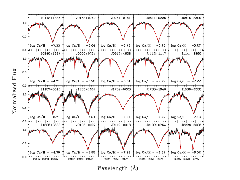
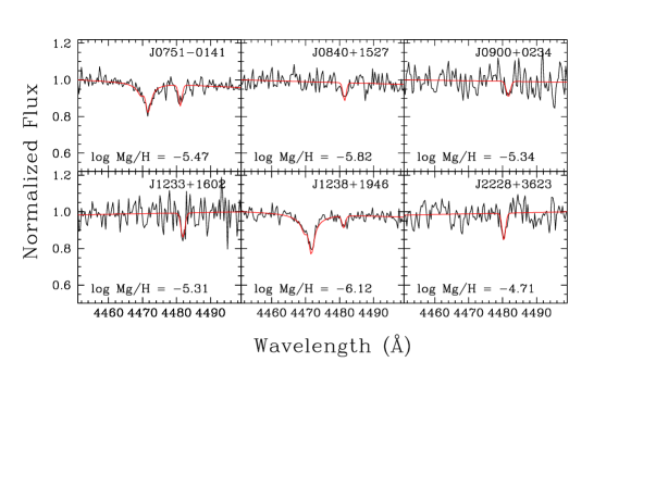
Figure -1.— Fits of the Ca II H and K lines. Note that the H line (Ca ii $\lambda$3968) is blended with H$\epsilon$. The measured Ca abundance for each ELM WD is indicated in the individual panels.

Figure 0.— Same as Figure ‣ 4.1 but for the Mg ii $\lambda$4481 doublet. In the panels for J0751, and J1238 the He ii $\lambda$4471 line can also be observed.

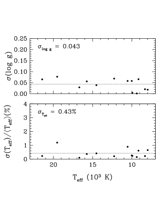
Figure 1.— Distribution of standard deviations in $T_{\rm eff}$ and $\log g$ for individual ELM WDs with multiple measurements as a function of $T_{\rm eff}$. Standard deviations in $T_{\rm eff}$ are expressed in percentage with respect to the average temperature of the star. The dotted lines represent the average standard deviations as indicated in the top left of each panel.

Figure 2.— Derivative of the equivalent width of H$\gamma$, H$\delta$, and H$\epsilon$ with respect to $T_{\rm eff}$ as a function of the effective temperature for models of ELM WDs. The surface gravity is held fixed here at a value of $\log g$ = 6.0.

Table 2ELM WD Binary Parameters

SDSS	$P$		$K$		Mass Function		$M_{2}$		$M_{2,i=60^{\circ}}$		$\tau_{\rm merge}$	$a$		$\log h$
	(days)		(km s-1)		($M_{\odot}$)		($M_{\odot}$)		($M_{\odot}$)		(Gyr)	($R_{\odot}$)
J0022+0031	0.49135 $\pm$	0.02540	80.8 $\pm$	1.3	0.027 $\pm$	0.003	$\geqslant$0.23 $\pm$	0.02	0.28 $\pm$	0.02	…	2.32 $\pm$	0.12	$-$22.79
J0022$-$1014	0.07989 $\pm$	0.00300	145.6 $\pm$	5.6	0.026 $\pm$	0.004	$\geqslant$0.20 $\pm$	0.02	0.25 $\pm$	0.02	$\leqslant$ 0.616	0.65 $\pm$	0.03	$-$22.55
J0056$-$0611	0.04338 $\pm$	0.00002	376.9 $\pm$	2.4	0.241 $\pm$	0.005	$\geqslant$0.46 $\pm$	0.02	0.61 $\pm$	0.03	$\leqslant$ 0.120	0.45 $\pm$	0.01	$-$22.06
J0106$-$1000	0.02715 $\pm$	0.00002	395.2 $\pm$	3.6	0.174 $\pm$	0.005	$\geqslant$0.39 $\pm$	0.02	0.51 $\pm$	0.03	$\leqslant$ 0.036	0.32 $\pm$	0.01	$-$22.61
J0112+1835	0.14698 $\pm$	0.00003	295.3 $\pm$	2.0	0.392 $\pm$	0.008	$\geqslant$0.62 $\pm$	0.03	0.85 $\pm$	0.04	$\leqslant$ 2.650	1.08 $\pm$	0.02	$-$22.41
J0152+0749	0.32288 $\pm$	0.00014	217.0 $\pm$	2.0	0.342 $\pm$	0.010	$\geqslant$0.57 $\pm$	0.03	0.78 $\pm$	0.04	…	1.79 $\pm$	0.04	$-$22.81
J0345+1748	0.23503 $\pm$	0.00013	273.4 $\pm$	0.5	0.498 $\pm$	0.003	$\geqslant$0.81 $\pm$	0.03	0.72 $\pm$	0.01a	$\leqslant$ 5.742	1.62 $\pm$	0.02	$-$21.97
J0651+2844	0.00886 $\pm$	0.00001	616.9 $\pm$	5.0	0.215 $\pm$	0.005	$\geqslant$0.49 $\pm$	0.02	0.50 $\pm$	0.04a	$\leqslant$ 0.001	0.16 $\pm$	0.01	$-$21.97
J0730+1703	0.69770 $\pm$	0.05427	122.8 $\pm$	4.3	0.134 $\pm$	0.025	$\geqslant$0.33 $\pm$	0.05	0.42 $\pm$	0.07	…	2.64 $\pm$	0.26	$-$23.48
J0745+1949	0.11240 $\pm$	0.00833	108.7 $\pm$	2.9	0.015 $\pm$	0.002	$\geqslant$0.10 $\pm$	0.01	0.12 $\pm$	0.02	$\leqslant$ 5.448	0.63 $\pm$	0.06	$-$22.49
J0751$-$0141	0.08001 $\pm$	0.00279	432.6 $\pm$	2.3	0.671 $\pm$	0.034	$\geqslant$0.97 $\pm$	0.06	0.97 $\pm$	0.04a	$\leqslant$ 0.320	0.82 $\pm$	0.04	$-$22.77
J0755+4800	0.54627 $\pm$	0.00522	194.5 $\pm$	5.5	0.416 $\pm$	0.039	$\geqslant$0.89 $\pm$	0.07	1.17 $\pm$	0.09	…	3.07 $\pm$	0.09	$-$21.75
J0755+4906	0.06302 $\pm$	0.00213	438.0 $\pm$	5.0	0.549 $\pm$	0.037	$\geqslant$0.81 $\pm$	0.06	1.13 $\pm$	0.09	$\leqslant$ 0.210	0.66 $\pm$	0.03	$-$22.64
J0802$-$0955	0.54687 $\pm$	0.00455	176.5 $\pm$	4.5	0.312 $\pm$	0.026	$\geqslant$0.58 $\pm$	0.05	0.77 $\pm$	0.07	…	2.60 $\pm$	0.09	$-$23.01
J0811+0225	0.82194 $\pm$	0.00049	220.7 $\pm$	2.5	0.915 $\pm$	0.032	$\geqslant$1.21 $\pm$	0.06	1.72 $\pm$	0.08	…	4.12 $\pm$	0.08	$-$23.17
J0815+2309	1.07357 $\pm$	0.00018	131.7 $\pm$	2.6	0.254 $\pm$	0.015	$\geqslant$0.50 $\pm$	0.04	0.67 $\pm$	0.05	…	3.94 $\pm$	0.11	$-$23.43
J0818+3536	0.18315 $\pm$	0.02110	170.0 $\pm$	5.0	0.093 $\pm$	0.019	$\geqslant$0.25 $\pm$	0.04	0.33 $\pm$	0.06	$\leqslant$ 9.269	1.02 $\pm$	0.13	$-$23.48
J0822+2753	0.24400 $\pm$	0.00020	271.1 $\pm$	9.0	0.504 $\pm$	0.051	$\geqslant$0.78 $\pm$	0.08	1.07 $\pm$	0.11	$\leqslant$ 7.529	1.62 $\pm$	0.06	$-$22.16
J0825+1152	0.05819 $\pm$	0.00001	319.4 $\pm$	2.7	0.196 $\pm$	0.005	$\geqslant$0.49 $\pm$	0.02	0.64 $\pm$	0.03	$\leqslant$ 0.158	0.58 $\pm$	0.01	$-$22.45
J0840+1527	0.52155 $\pm$	0.00474	84.8 $\pm$	3.1	0.033 $\pm$	0.004	$\geqslant$0.16 $\pm$	0.02	0.20 $\pm$	0.02	…	1.92 $\pm$	0.08	$-$24.19
J0845+1624	0.75599 $\pm$	0.02164	62.2 $\pm$	5.4	0.019 $\pm$	0.005	$\geqslant$0.19 $\pm$	0.03	0.23 $\pm$	0.04	…	2.99 $\pm$	0.13	$-$23.12
J0849+0445	0.07870 $\pm$	0.00010	366.9 $\pm$	4.7	0.403 $\pm$	0.016	$\geqslant$0.65 $\pm$	0.04	0.89 $\pm$	0.05	$\leqslant$ 0.441	0.73 $\pm$	0.02	$-$22.38
J0900+0234	…		$\leqslant$24.0		…		…		…		…	…		…
J0917+4638	0.31642 $\pm$	0.00002	148.8 $\pm$	2.0	0.108 $\pm$	0.004	$\geqslant$0.28 $\pm$	0.02	0.36 $\pm$	0.02	…	1.50 $\pm$	0.04	$-$23.33
J0923+3028	0.04495 $\pm$	0.00049	296.0 $\pm$	3.0	0.121 $\pm$	0.005	$\geqslant$0.37 $\pm$	0.02	0.47 $\pm$	0.03	$\leqslant$ 0.102	0.46 $\pm$	0.01	$-$21.58
J1005+0542	0.30560 $\pm$	0.00007	208.9 $\pm$	6.8	0.289 $\pm$	0.028	$\geqslant$0.70 $\pm$	0.05	0.91 $\pm$	0.07	$\leqslant$ 7.696	1.96 $\pm$	0.04	$-$22.38
J1005+3550	0.17652 $\pm$	0.00011	143.0 $\pm$	2.3	0.053 $\pm$	0.003	$\geqslant$0.19 $\pm$	0.02	0.24 $\pm$	0.02	$\leqslant$10.448	0.94 $\pm$	0.03	$-$23.13
J1046$-$0153	0.39539 $\pm$	0.10836	80.8 $\pm$	6.6	0.022 $\pm$	0.011	$\geqslant$0.19 $\pm$	0.05	0.23 $\pm$	0.06	…	1.87 $\pm$	0.42	$-$22.58
J1053+5200	0.04256 $\pm$	0.00002	264.0 $\pm$	2.0	0.081 $\pm$	0.002	$\geqslant$0.26 $\pm$	0.01	0.33 $\pm$	0.02	$\leqslant$ 0.147	0.40 $\pm$	0.01	$-$22.50
J1056+6536	0.04351 $\pm$	0.00103	267.5 $\pm$	7.4	0.086 $\pm$	0.009	$\geqslant$0.34 $\pm$	0.03	0.43 $\pm$	0.04	$\leqslant$ 0.085	0.46 $\pm$	0.02	$-$22.33
J1104+0918	0.55319 $\pm$	0.00502	142.1 $\pm$	6.0	0.164 $\pm$	0.022	$\geqslant$0.55 $\pm$	0.05	0.69 $\pm$	0.07	…	2.84 $\pm$	0.08	$-$21.88
J1112+1117	0.17248 $\pm$	0.00001	116.2 $\pm$	2.8	0.028 $\pm$	0.002	$\geqslant$0.14 $\pm$	0.01	0.17 $\pm$	0.02	$\leqslant$12.019	0.89 $\pm$	0.03	$-$22.51
J1141+3850	0.25958 $\pm$	0.00005	265.8 $\pm$	3.5	0.505 $\pm$	0.020	$\geqslant$0.76 $\pm$	0.05	1.06 $\pm$	0.06	$\leqslant$ 9.518	1.68 $\pm$	0.04	$-$23.36
J1151+5858	0.66902 $\pm$	0.00070	175.7 $\pm$	5.9	0.376 $\pm$	0.038	$\geqslant$0.63 $\pm$	0.06	0.85 $\pm$	0.09	…	3.00 $\pm$	0.11	$-$23.45
J1157+0546	0.56500 $\pm$	0.01925	158.3 $\pm$	4.9	0.232 $\pm$	0.030	$\geqslant$0.46 $\pm$	0.05	0.61 $\pm$	0.07	…	2.49 $\pm$	0.15	$-$23.98
J1233+1602	0.15090 $\pm$	0.00009	336.0 $\pm$	4.0	0.593 $\pm$	0.022	$\geqslant$0.85 $\pm$	0.05	1.19 $\pm$	0.06	$\leqslant$ 2.161	1.20 $\pm$	0.03	$-$23.03
J1234$-$0228	0.09143 $\pm$	0.00400	94.0 $\pm$	2.3	0.008 $\pm$	0.001	$\geqslant$0.09 $\pm$	0.01	0.11 $\pm$	0.01	$\leqslant$ 2.606	0.59 $\pm$	0.03	$-$22.89
J1238+1946	0.22275 $\pm$	0.00009	258.6 $\pm$	2.5	0.399 $\pm$	0.012	$\geqslant$0.68 $\pm$	0.03	0.92 $\pm$	0.04	$\leqslant$ 5.871	1.49 $\pm$	0.03	$-$23.11
J1422+4352	0.37930 $\pm$	0.01123	176.0 $\pm$	6.0	0.214 $\pm$	0.028	$\geqslant$0.42 $\pm$	0.05	0.56 $\pm$	0.07	…	1.86 $\pm$	0.11	$-$23.29
J1436+5010	0.04580 $\pm$	0.00010	347.4 $\pm$	8.9	0.199 $\pm$	0.016	$\geqslant$0.45 $\pm$	0.04	0.59 $\pm$	0.05	$\leqslant$ 0.107	0.47 $\pm$	0.01	$-$22.13
J1439+1002	0.43741 $\pm$	0.00169	174.0 $\pm$	2.0	0.239 $\pm$	0.009	$\geqslant$0.47 $\pm$	0.03	0.62 $\pm$	0.04	…	2.10 $\pm$	0.06	$-$22.84
J1443+1509	0.19053 $\pm$	0.02402	306.7 $\pm$	3.0	0.569 $\pm$	0.089	$\geqslant$0.86 $\pm$	0.12	1.19 $\pm$	0.17	$\leqslant$ 3.403	1.42 $\pm$	0.18	$-$22.10
J1448+1342	…		$\leqslant$35.0		…		…		…		…	…		…
J1512+2615	0.59999 $\pm$	0.02348	115.0 $\pm$	4.0	0.095 $\pm$	0.014	$\geqslant$0.31 $\pm$	0.03	0.39 $\pm$	0.04	…	2.47 $\pm$	0.14	$-$22.95
J1518+0658	0.60935 $\pm$	0.00004	172.0 $\pm$	2.0	0.321 $\pm$	0.011	$\geqslant$0.60 $\pm$	0.03	0.81 $\pm$	0.04	…	2.84 $\pm$	0.06	$-$22.33
J1538+0252	0.41915 $\pm$	0.00295	227.6 $\pm$	4.9	0.512 $\pm$	0.037	$\geqslant$0.76 $\pm$	0.06	1.06 $\pm$	0.09	…	2.30 $\pm$	0.08	$-$22.87
J1557+2823	0.40741 $\pm$	0.00294	131.2 $\pm$	4.2	0.095 $\pm$	0.010	$\geqslant$0.42 $\pm$	0.03	0.52 $\pm$	0.04	…	2.22 $\pm$	0.05	$-$21.91
J1614+1912	…		$\leqslant$56.0		…		…		…		…	…		…
J1625+3632	0.23238 $\pm$	0.03960	58.4 $\pm$	2.7	0.005 $\pm$	0.001	$\geqslant$0.07 $\pm$	0.01	0.09 $\pm$	0.02	…	1.04 $\pm$	0.16	$-$23.95
J1630+2712	0.27646 $\pm$	0.00002	218.0 $\pm$	5.0	0.297 $\pm$	0.020	$\geqslant$0.52 $\pm$	0.04	0.70 $\pm$	0.06	…	1.58 $\pm$	0.05	$-$23.14
J1630+4233	0.02766 $\pm$	0.00004	295.9 $\pm$	4.9	0.074 $\pm$	0.004	$\geqslant$0.30 $\pm$	0.02	0.38 $\pm$	0.02	$\leqslant$ 0.031	0.33 $\pm$	0.01	$-$22.03
J1741+6526	0.06111 $\pm$	0.00001	508.0 $\pm$	4.0	0.830 $\pm$	0.020	$\geqslant$1.10 $\pm$	0.05	1.57 $\pm$	0.06	$\leqslant$ 0.160	0.71 $\pm$	0.01	$-$22.12
J1840+6423	0.19130 $\pm$	0.00005	272.0 $\pm$	2.0	0.399 $\pm$	0.009	$\geqslant$0.65 $\pm$	0.03	0.89 $\pm$	0.04	$\leqslant$ 4.579	1.32 $\pm$	0.03	$-$22.37
J2103$-$0027	0.20308 $\pm$	0.00023	281.0 $\pm$	3.2	0.467 $\pm$	0.016	$\geqslant$0.71 $\pm$	0.04	0.98 $\pm$	0.05	$\leqslant$ 5.683	1.39 $\pm$	0.03	$-$22.74
J2119$-$0018	0.08677 $\pm$	0.00004	383.0 $\pm$	4.0	0.505 $\pm$	0.016	$\geqslant$0.74 $\pm$	0.04	1.04 $\pm$	0.05	$\leqslant$ 0.574	0.80 $\pm$	0.02	$-$22.84
J2132+0754	0.25056 $\pm$	0.00002	297.3 $\pm$	3.0	0.682 $\pm$	0.021	$\geqslant$0.96 $\pm$	0.05	1.34 $\pm$	0.06	$\leqslant$ 7.337	1.74 $\pm$	0.03	$-$22.62
J2228+3623	…		$\leqslant$28.0		…		…		…		…	…		…
J2236+2232	1.01016 $\pm$	0.00005	119.9 $\pm$	2.0	0.180 $\pm$	0.009	$\geqslant$0.39 $\pm$	0.03	0.51 $\pm$	0.04	…	3.52 $\pm$	0.10	$-$22.80
J2252$-$0056	…		$\leqslant$25.0		…		…		…		…	…		…
J2338$-$2052	0.07644 $\pm$	0.00712	133.4 $\pm$	7.5	0.019 $\pm$	0.005	$\geqslant$0.15 $\pm$	0.02	0.18 $\pm$	0.03	$\leqslant$ 0.972	0.56 $\pm$	0.05	$-$22.86
J2345$-$0102	…		$\leqslant$43.0		…		…		…		…	…		…
aEclipsing systems where we adopt $M_{2}$ and $i$ as determined from the eclipse modeling (see Section 4.2) instead of assuming $i=60^{\circ}$.

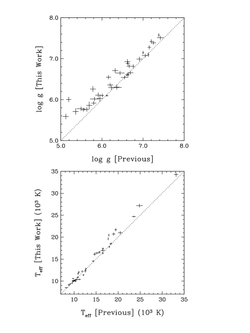
Figure 3.— Comparison of the atmospheric parameters $T_{\rm eff}$ (bottom) and $\log g$ (top) presented in this work to those published in previous analyses (see Table 5 of Brown et al. 2013, and references therein). In both panels, the dashed line represents the 1:1 correlation.

Table 3Measured Atmospheric Abundances

SDSS	$\log$ (He/H)	$\log$ (Mg/H)	$\log$ (Ca/H)
J0112+1835	…	…	$-$7.33
J0152+0749	…	…	$-$8.64
J0745+1949	…	$-$3.90	$-$5.80
J0751$-$0141	$-$1.28	$-$5.47	$-$6.73
J0811+0225	…	…	$-$5.28
J0815+2309	…	…	$-$5.27
J0840+1527	…	$-$5.82	$-$4.71
J0900+0234	…	$-$5.34	$-$6.92
J0917+4638	…	…	$-$5.54
J1112+1117	…	…	$-$7.22
J1141+3850	$-$0.53	…	$-$7.22
J1157+0546	$-$0.55	…	$-$5.71
J1233+1602	…	$-$5.31	$-$5.24
J1234$-$0228	…	…	$-$6.81
J1238+1946	$-$0.67	$-$6.12	$-$6.02
J1538+0252	…	…	$-$7.18
J1625+3632	$-$3.02	…	$-$4.39
J2103$-$0027	…	…	$-$6.95
J2119$-$0018	…	…	$-$7.28
J2132+0754	…	…	$-$6.12
J2228+3623	…	$-$4.71	$-$6.52

The results of our Balmer line fits using our pure hydrogen grid are displayed in Figure 3.3. For the five ELM WDs which also have helium lines in their optical spectra, we proceed using the exact same approach detailed above but in addition to the Balmer lines, we also fit two neutral helium lines, namely He i $\lambda$4471 and He i $\lambda$4026 in order to measure the helium abundance. Our fits to the these five objects are displayed in Figure -2.

For the fits to the Ca ii $\lambda$3968 H & Ca ii $\lambda$3934 K lines and the Mg ii $\lambda$4481 doublet, $T_{\rm eff}$ and $\log g$ are kept fixed at the values measured from the Balmer line fits and only the Ca and Mg abundances are allowed to vary. The results of the Ca and Mg line fits are shown in Figures ‣ 4.1 and ‣ 4.1, respectively.

Finally, the only ELM WD whose fit is not shown in Figures 3.3 through ‣ 4.1 is that of the metal-rich and tidally distorted ELM WD binary J0745. We refer the reader to Gianninas et al. (2014) for a detailed description of the analysis of J0745.

4.2. Adopted Physical and Binary Parameters

We present in Table 1 our adopted atmospheric parameters for the 61 ELM WDs in our sample based on the spectroscopic analysis presented in the previous section. In the first column we list the abbreviated SDSS name for each object, ordered by right ascension, followed by our spectroscopically determined values of $T_{\rm eff}$ and $\log g$ with their associated uncertainties. Our error estimates combine the statistical error of the model fits, obtained from the covariance matrix of the fitting algorithm, and the systematic error.

The systematic uncertainties for WDs with $\log g$ $\sim$ 8.0 have been estimated by Liebert et al. (2005) using multiple observations of the same object and are typically 1.2% in $T_{\rm eff}$ and 0.038 dex in $\log g$. However, it is not immediately obvious that these estimates apply to ELM WDs with $\log g$ $\sim$ 5–6. We have therefore performed an analogous analysis to that shown in Figure 8 of Liebert et al. (2005) using instead the 13 ELM WDs for which we have multiple observations – obtained independently at the MMT and FLWO using the distinct instrument setups described in Section 2 – to calculate the average parameters and standard deviation for each star. The results of this exercise are displayed in 1 as a function of $T_{\rm eff}$. The average standard deviation in $\log g$ is 0.043 dex. This is quite comparable to the value of 0.038 dex determined by Liebert et al. (2005). On the other hand, we obtain a standard deviation of 0.43% in $T_{\rm eff}$.

We display in Figure 2 the sensitivity of the equivalent width ($W$) of H$\gamma$, H$\delta$, and H$\epsilon$ to variations of $T_{\rm eff}$ (i.e. $dW/d$$T_{\rm eff}$) as a function of $T_{\rm eff}$ for models with $\log g$ = 6.0. We did not consider H$\beta$ since it is not included in our fits. If we compare this result with that obtained for $\log g$ = 8.0 (see Figure 1 in Fontaine et al. 2003) we first remark that the temperature where the sensitivity vanishes (i.e. where the Balmer lines reach their maximum equivalent width and $dW/d$$T_{\rm eff}$ = 0) has shifted from $\approx$13,500 K down to $\approx$10,500 K. However, to either side of this value, the Balmer lines are just as sensitive at $\log g$ = 6.0 as they are at $\log g$ = 8.0. Therefore, it is not surprising that we achieve a similar precision.

We must also point out that there is an additional source of uncertainty in the atmospheric parameters, and all the quantities derived from them, due to the unknown contribution to the optical spectrum from the companion. Given that these are all single-lined systems (unlike SDSS 1257+5428, see Kulkarni & van Kerkwijk 2010) whose companions are likely more massive, cooler, and hence less luminous WDs, we expect their contribution to the observed spectrum to be on the order of a few percent at most. For example, Hermes et al. (2012c) estimated that the companion of J0651 contributes $\approx$ 4% of the flux in the SDSS $g$-band (centered at $\lambda\approx$ 4686 Å). The contamination is mitigated by the fact that we restrict our fits to the region blueward of H$\beta$ ($\lambda<$ 4500 Å) where a cooler WD would only contribute a small fraction of the observed flux. However, since it is impossible to constrain the parameters ($T_{\rm eff}$, $\log g$) of the unseen companions with our current data, this remains an additional source of uncertainty. As a result, we choose to adopt the slightly more conservative uncertainties from Liebert et al. (2005).

Table 1 also lists the stellar mass and stellar radius of the primary as determined by coupling our $T_{\rm eff}$ and $\log g$ determinations with the evolutionary models of Althaus et al. (2013) appropriate for low mass He-core WDs. The only exception is J2345$-$0102 whose $T_{\rm eff}$ and $\log g$ formally place it outside the Althaus grid. For this object, we use the evolutionary models of Panei et al. (2007) instead. The formal uncertainty in the stellar mass is obtained by considering the uncertainties on $T_{\rm eff}$ and $\log g$ as well as the uncertainties from the evolutionary models (see Althaus et al. 2013, for a detailed discussion). However, there remains sufficient uncertainty in the masses derived from the Althaus et al. (2013) models due in large part to the many H shell flashes predicted for the models with masses in the range 0.18–0.36 $M_{\odot}$. For this reason, we adopt a more conservative uncertainty of 0.020 $M_{\odot}$ for all of our mass estimates.

The next column lists $g_{0}$, the extinction corrected SDSS $g$-band magnitude from Data Release 10 (Ahn et al. 2014) followed by $M_{g}$ the absolute magnitude determined using the photometric calibrations of Holberg & Bergeron (2006). The second-to-last column combines the apparent and absolute magnitudes to provide an estimate of the distance in kpc. Finally, in the last column, we list the cooling age, $\tau_{\rm cool}$, which we again infer from the models of Althaus et al. (2013). We note again that the parameters for J0745 are taken from Gianninas et al. (2014).

In Table 2 we provide the binary parameters based on our updated atmospheric parameters. First, we list the orbital period, $P$, and velocity semi-amplitude, $K$, for each system. Based on these values we compute the mass function of the system. Next, we use the mass function to compute the minimum companion mass, $M_{2}$, assuming an orbital inclination angle of $i=90^{\circ}$, and the most likely companion mass by taking $i=60^{\circ}$, except for the three eclipsing systems discussed below. We also provide the merger times for those systems that will merge within a Hubble time. The last two columns provide the orbital separation and the expected gravitational wave strain. Note that no significant radial velocity variability has been observed for six ELM WDs in our sample and only upper limits on their velocity semi-amplitudes are provided. Consequently, we cannot provide binary parameters for those six systems.

There are three eclipsing systems in our sample: NLTT 11748, J0651, J0751 (Kaplan et al. 2014b; Brown et al. 2011; Kilic et al. 2014b, respectively) for which eclipse modeling provides model independent measurements of the parameters of the system. In particular, the orbital inclination angle and the mass of the secondary can be constrained and we adopt these values as the most likely secondary mass for these three objects. Both J0651 and J0751 have $i\approx 85^{\circ}$ and it is not surprising that the secondary masses derived from modeling their eclipses, $M_{2,{\rm eclipse}}$ = 0.50 $M_{\odot}$ and 0.97 $M_{\odot}$, respectively, are in excellent agreement with the minimum secondary masses of $M_{2}$ = 0.49 $\pm$ 0.02 $M_{\odot}$ and 0.97 $\pm$ 0.06 $M_{\odot}$, respectively, computed assuming $i$ = 90^∘. On the other hand, Kaplan et al. (2014b) measured $i$ = 89.67^∘ $\pm$ 0.12^∘ for NLTT 11748 and obtain $M_{2,{\rm eclipse}}$ = 0.72 $\pm$ 0.01 $M_{\odot}$ which is significantly different from our determination of $M_{2}$ = 0.81 $\pm$ 0.02 $M_{\odot}$. Since our determination of the companion mass depends on the mass of the primary, via the mass function, the disagreement between our determination and that of Kaplan et al. (2014b) is another symptom of high $\log g$ problem discussed in detail below (see Section 5.3).

Finally, Table 3 summarizes the measured atmospheric abundances of He, Mg, and Ca. As in Gianninas et al. (2014), we adopt uncertainties of 0.30 dex for all the abundances listed in Table 3. This large uncertainty stems from the fact that we are only fitting a single Ca, or Mg, line at fixed values of $T_{\rm eff}$ and $\log g$.

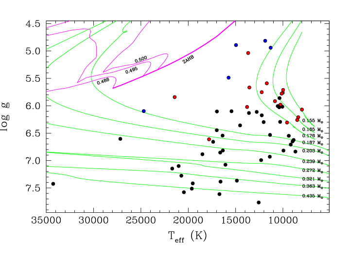
Figure 4.— The location of the 61 ELM WDs in our sample in the $T_{\rm eff}$-$\log g$ plane. The red circles correspond to ELM WDs with Ca lines whereas the blue dots denote ELM WDs which have both Ca and He lines. The solid green lines correspond to theoretical evolutionary tracks for 0.155–0.435 $M_{\odot}$ He-core WDs from Althaus et al. (2013). Also shown as the solid magenta lines are horizontal branch tracks for 0.488, 0.495 and 0.500 $M_{\odot}$ stars from Dorman et al. (1993) as well as the zero-age horizontal branch (ZAHB) represented by the thick magenta line.

In Figure 3, we show a comparison of the atmospheric parameters from this work compared to those published in the previous ELM survey papers. In the bottom panel, we see that $T_{\rm eff}$ matches particularly well for lower values, while previous analyses yield somewhat lower $T_{\rm eff}$ at higher values. A somewhat more pronounced difference is noticeable in the comparison of surface gravities. The new $\log g$ values we obtained are almost systematically higher than those from previous work. Both of these trends are almost certainly due to the fact that the models used in previous analyses did not included the new Stark broadening tables from Tremblay & Bergeron (2009). The inclusion of these new calculations has already been shown to produce exactly the same systematic shift of the atmospheric parameters when compared to the previous generation of models (see Figure 9 of Gianninas et al. 2011).

5. Discussion

5.1. Metals in ELM WDs

We plot in Figure 4 our entire sample of ELM WDs in the $T_{\rm eff}$-$\log g$ plane. As a guide, we also plot the evolutionary tracks for He-core WDs from Althaus et al. (2013). Note that, in the interest of clarity, only the final cooling portion of the Althaus tracks are shown; we omit the H-shell flashes for models between 0.187 and 0.363 $M_{\odot}$. We also plot horizontal branch tracks with [Fe/H] = $-$1.48 from Dorman et al. (1993) for 0.488, 0.495, and 0.500 $M_{\odot}$ stars as well as the zero-age horizontal branch. We can see that the WDs from the ELM Survey lie in a region where we only expect He-core WDs to be found. Figure 4 also reveals that nearly all the ELM WDs with $\log g$ $<$ 6.0 are polluted with Ca. The only exception to this rule is J0818+3536. However, the spectrum of J0818+3536 has a S/N = 17 (see the second panel of Figure 3.3). The noise level in the continuum between H$\epsilon$ and H8 could easily conceal a weak Ca line. It seems therefore that the presence of metals in the lowest mass ELM WDs is a rather ubiquitous phenomenon and possibly linked to the evolution of these objects.

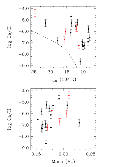
Figure 5.— Measured Ca abundances plotted as a function of $T_{\rm eff}$ (top) and stellar mass (bottom). Red triangles represent ELM WDs which also contain He. The dashed line corresponds to the detection threshold for Ca lines in our spectra.

Figure 6.— Measured Mg abundances plotted as a function of $T_{\rm eff}$.

In Figure 5, we plot the measured Ca abundances as a function of both $T_{\rm eff}$ (top) and the stellar mass (bottom). ELM WDs which also contain helium are shown in red. Kaplan et al. (2013) suggested that H-shell flashes may mix the interior of the WD subsequently bringing metals back to the surface. We would then expect that as the WD cools and shell flashes cease, the metals would simply diffuse out of the atmosphere leading to increasingly lower abundances as a function of $T_{\rm eff}$. However, the overall distribution of Ca abundances in the upper panel of Figure 5 does not display any obvious trend. A simple linear fit to the data yields a $p$-value of 0.011. A similar analysis of the data in the lower panel of Figure 5 gives $p$ = 0.069. These results indicate that the Ca abundance distributions are not strongly correlated to either $T_{\rm eff}$ or the mass of the WD. Finally, we also show in Figure 5 an estimate of the detection limit for Ca. Taking into account the typical S/N and resolution of our spectra, we estimate a minimum equivalent width of 40 mÅ for Ca lines to be detectable. Our measured Ca abundances are consistent with this detection limit.

The distribution of Mg abundances as a function of $T_{\rm eff}$ is plotted in Figure 6. A linear fit in this case produces $p$ = 0.046, once again indicating that there is no strong correlation. In any case, with only seven Mg detections, as well as the large uncertainties, it would be difficult to draw any meaningful conclusions.

The shell flash scenario is also at odds with the fact that metals are observed in ELM WDs where the evolutionary models do not predict shell flashes (i.e. for $M<$ 0.18 $M_{\odot}$). This inconsistency suggests that the evolutionary models are possibly in error. On the other hand, since we have adopted an uncertainty of 0.02 $M_{\odot}$ for our mass estimates, it’s entirely possible that the true mass of these objects places them in the regime where shell flashes do indeed occur.

Another difficulty with the shell flash scenario is that the diffusion timescales for metals in the atmospheres of WDs is typically much shorter than the evolutionary timescale (Paquette et al. 1986; Koester & Wilken 2006), even in ELM WDs (Hermes et al. 2014b). Even if shell flashes are the mechanism bringing metals to the surface, some other physical process must be working to keep them in the atmosphere. It is possible that radiative levitation could act against gravitational settling (Chayer & Dupuis 2010; Dupuis et al. 2010; Chayer 2014). It is not yet clear if the considerably lower surface gravity in ELM WDs would allow radiative levitation to support metals in the atmosphere. Detailed calculations of radiative levitation in ELM WDs will need to be performed to explore this possibility (Hermes et al. 2014b).

In canonical mass WDs, the presence of metals has been successfully shown to be the result of ongoing accretion from circumstellar debris disks formed by the tidal disruption of planetary bodies (Debes & Sigurdsson 2002; Farihi et al. 2010a, b; Jura 2003, 2006, 2008; Jura et al. 2007; Melis et al. 2010). These are detected through excess flux in the IR (Jura 2003; Kilic et al. 2006; Farihi et al. 2009; Barber et al. 2012). In the case of ELM WDs, due to the close nature of these binary systems, we would expect that any disks would in fact be circumbinary. However, the formation of such circumbinary disks is problematic. The Roche radius of a WD is typically $\sim$ 1.0–1.5 $R_{\odot}$ (Jura 2003; von Hippel et al. 2007; Rafikov 2011). The critical radius for stable orbits around a circularized binary is $\sim$2 times the orbital separation (Holman & Wiegert 1999). As it turns out, of the 20 metal-rich ELM WDs, only J0745 has and orbital separation (0.63 $\pm$ 0.06 $R_{\odot}$) small enough to allow for an orbiting body to pass within its Roche radius. There is currently no evidence for debris disks around ELM WDs and the orbital separations for virtually all the metal-rich WDs rules out the debris disk scenario to explain the presence of metals in ELM WDs.

The ongoing efforts of the ELM Survey will be crucial in increasing the sample size of these metal-rich ELM WDs. In addition, detailed analyses based on high-resolution spectroscopy of metal-rich ELM WDs would allow for more accurate abundance measurements. If multiple metal lines are detected, and three parameter fits are performed (i.e. $T_{\rm eff}$, $\log g$, and abundances), this would greatly increase the precision and accuracy of the measured abundances. Until such observations and studies are performed, it will remain difficult to draw any firm conclusions regarding the origin of metals in the atmospheres of ELM WDs.

5.2. Helium in ELM WDs

In addition to Ca and Mg, five ELM WDs have optical spectra where we observe He lines. It is interesting to note that with the exception of J1625+3632 at $T_{\rm eff}$ $\approx$ 25,000 K, the remaining four ELM WDs are clustered together at low $\log g$ in Figure 4. These are also the four WDs with the highest measured He abundances in our sample. Indeed, the measured He abundances (see Table 3) for J1141+3850, J1157+0546, and J1239+1946 are unusually high with $\log$ (He/H) $\approx$ $-0.5$. The ELM WD companion to PSR J1816+4510 (Kaplan et al. 2013) with $T_{\rm eff}$ = 16,000 $\pm$ 500 K, $\log g$ = 4.9 $\pm$ 0.3, and $\log$ (He/H) = 0.0 $\pm$ 0.5 is another example of an ELM WD with very similar atmospheric parameters. Althaus et al. (2013) report that the predicted shell flashes “markedly reduce the hydrogen content of the star” through a rapid and intense episode of CNO burning, producing He in the process. We postulate that the presence of important quantities of He, not metals, could very well be the signature of a recent shell flash.

Figure 7.— Differences in stellar radii as determined from our spectroscopic analysis ($R_{spec}$) and from light curve analyses ($R_{phot}$), in units of $R_{\odot}$, plotted as a function of $T_{\rm eff}$. The error bars represent the errors of the two independent radius measurements combined in quadrature. As a guide, we plot as a dotted line the locus where both the independent radius measurements are equal.

5.3. Radius Comparison

Model independent measurements of stellar parameters are crucial for testing the validity of theoretical models. The nature of several ELM WD binaries afford us just such a possibility. Ellipsoidal variations due to tidal distortions and eclipse modeling provide model-independent measurements of the stellar radius. There are three eclipsing ELM WDs in the sample analyzed here, J0651, J0751, and NLTT 11748 (Hermes et al. 2012c; Kilic et al. 2014b; Kaplan et al. 2014b, respectively). Several other eclipsing ELM WDs have been discovered as well including GALEX J1717+6757 (Vennes et al. 2011) and CSS 41177 (Bours et al. 2014). Furthermore, there are eight ELM WDs which show photometric variability attributed to ellipsoidal variations. These include J0745 (Gianninas et al. 2014) and seven more systems analyzed in Hermes et al. (2014b). Note that J0651 and J0751 both display ellipsoidal variations and eclipses in their observed light curves. Finally, the ELM WD LP 400-22, a unique system that is leaving the galaxy, has a measured parallax which also constrains the radius of the star (Kilic et al. 2013b).

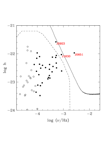
Figure 8.— Gravitational wave strain versus frequency for our ELM WD binaries. Filled circles represent merger systems whereas open circles correspond to non-merger systems. The solid line represents the new sensitivity curve for of $eLISA$ after two years of observation (Amaro-Seoane et al. 2013). The dashed line shows the predicted average Galactic foreground after one year of integration (Nelemans et al. 2001). The three labeled objects are the ELM WD binaries which could be verification sources for $eLISA$.

In Figure 7 we plot the difference in the determinations of the stellar radii for ELM WDs derived from our spectroscopic analysis and from the model-independent determinations enumerated above, as a function of $T_{\rm eff}$. We see that the agreement between the spectroscopically inferred radii and the model-independent values is quite good for $T_{\rm eff}$ $>$ 10,000 K, given the uncertainties. However, there are three objects where the radius estimates do not agree: NLTT 11748, LP 400-22, and J0745. In all three cases, the spectroscopic determination underestimates the radius. The result for NLTT 11748 in particular is 4$\sigma$ significance. In the case of J0745, it is possible that the spectroscopic mass and radius determinations suffer from the assumption that the WD is on its terminal cooling track (see Hermes et al. 2014b, for a detailed discussion). As for LP 400-22, its measured parallax implies a lower limit of $R$ = 0.099 $R_{\odot}$ (see Kilic et al. 2013b, for a detailed discussion).

Underestimating the radius is analogous to overestimating the mass or the surface gravity since WDs have an inverse mass-radius relationship. This is most likely a manifestation of the “high $\log g$ problem” (Kepler et al. 2007; Tremblay et al. 2010; Gianninas et al. 2011) but in the regime of ELM WDs, as first noted in Gianninas et al. (2014). This well documented phenomenon is a consequence of the 1D treatment of convection via the mixing-length theory (Tremblay et al. 2011), the same treatment currently implemented in the model grids used for our analysis. Tremblay et al. (2013a) presented a new series of models which employ a 3D hydrodynamical treatment of convection. Tremblay et al. (2013b) then showed how these models effectively solve the high $\log g$ problem and derive corrections which can be applied to atmospheric parameters determined from 1D models. Figure 4 in Tremblay et al. (2013b) shows these corrections which systematically imply lower $\log g$ values than those determined from 1D models. Unfortunately the model grid in Tremblay et al. (2013b) only extends to $\log g$ = 7.0 and therefore does not cover parameters appropriate for ELM WDs. However, we remark that the corrections for the models at $\log g$ = 7.0 are greatest for 10,000 K $>$ $T_{\rm eff}$ $>$ 8000 K. This roughly matches the range in $T_{\rm eff}$ where we see the largest discrepancy in our radius determinations. With only seven of our targets with $T_{\rm eff}$ $<$ 9500 K, only 11% of our sample is actually affected. We (in collaboration with P.-E. Tremblay) are currently computing 3D models appropriate for ELM WDs to resolve this issue.

5.4. Gravitational Waves

Using our determinations of the orbital period, distance and the masses of both components in our ELM WD binaries (assuming an inclination of $i=60^{\circ}$), we can calculate the gravitational wave strain, $h$, expected from these systems (see Roelofs et al. 2007, and references therein). The results of these calculations are listed in the last column of Table 2. We plot in Figure 8 $\log h$ as a function of $\log\nu$, where $\nu=2/P_{\rm orb}$ in Hz, for each system. The majority of our ELM WD binaries are contained within the region in Figure 8 characterizing the average galactic foreground emission predicted from population synthesis models (Nelemans et al. 2001). Our results suggest that an important fraction of the the galactic foreground at mHz frequencies is due to short-period ELM WD binaries. J0651 is the only ELM WD system that would be a verification source based on past $LISA$ sensitivity curves (Larson et al. 2000). Figure 8 shows that the new sensitivity curve for the revised $eLISA$ mission (Amaro-Seoane et al. 2013) leaves only three potentially viable sources. Note that the sensitivity curve shown here is expressed in terms of the dimensionless strain $h$ for monochromatic (periodic) sources for an integration time, $T$, of two years, i.e. the dimensionless value $\sqrt{S(f)/T}$, where $S(f)$ is the $eLISA$ equivalent-strain noise and $f$ is the frequency. However, the only real verification source remains J0651 as it lies well within the projected sensitivity region for $eLISA$. Given enough observation time and a high enough S/N, J0923 and J1630 could potentially be detected as well. As the ELM Survey is ongoing, there also remains a strong possibility that more verification binaries could be uncovered (e.g. Kilic et al. 2014a).

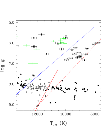
Figure 9.— Region of the $T_{\rm eff}$-$\log g$ plane containing the ZZ Ceti instability strip (lower left) and the five currently known ELM pulsators, which are labeled in the figure. Pulsators are identified as white diamonds whereas WDs which have been confirmed as photometrically constant are represented as black dots. The blue and red lines represent the empirical boundaries of the ZZ Ceti instability as determined by Gianninas et al. (2011). The dotted lines denote tentative boundaries which match the location of both instability strips. The green errorbars denote the remaining ELM WDs from our sample which have not yet been investigated for photometric variability.

5.5. Instability Strip

In this section, we use our new atmospheric parameter determinations to update the current view of the ELM WD instability strip for He-core pulsators and compare it with the most recent determination of the ZZ Ceti instability strip populated by CO-core WDs. In order to be able to make this comparison in a self-consistent manner, we plot in Figure 9 only WDs which have been analyzed using the exact same fitting technique used in the present analysis and using model atmospheres which employ the same parametrization of the mixing length theory to model convection (i.e. ML2/$\alpha$ = 0.8 Tremblay et al. 2010). For this reason, some of the WDs shown in Figure 5 of Hermes et al. (2013c) are not included here. For analogous reasons, we choose not to plot in Figure 9 the theoretically predicted boundaries of the extended ZZ Ceti instability computed by Van Grootel et al. (2013) since their pulsation models assume a parametrization of the mixing length theory equivalent to ML2/$\alpha$ = 0.6 in the atmosphere.

The lower portion of Figure 9 includes the 56 pulsating ZZ Ceti WDs as well as the 145 photometrically constant DA WDs from Gianninas et al. (2011). We also include GD 518, recently discovered to be the most massive known pulsating ZZ Ceti WD (Hermes et al. 2013a). The ELM WDs analyzed in this paper are represented in Figure 9 by analogous symbols with error bars. We plot the current sample of five ELM WD pulsators as well as non-variables listed in Hermes et al. (2012b, 2013b, 2013c). For the purposes of empirically defining the instability strip of ELM WDs, we consider the 20 ELM WDs analyzed by Hermes et al. (2014b) as non-variables from the point of view of pulsations. Their photometric variability is perfectly consistent with ellipsoidal variations and the observed periods correlate almost perfectly with the orbital periods. We also plot a number of additional non-variables ELM WDs from Steinfadt et al. (2010, 2012). Finally, ELM WDs which have not been observed for photometric variability are plotted as green error bars. Figure 9 clearly shows that the situation for ELM WD pulsators is not nearly as clear cut as it is for their more massive counterparts in the ZZ Ceti instability whose blue and red edges are fairly well constrained. However, if one extrapolates the empirical blue edge of the ZZ Ceti instability strip to lower $\log g$, the ELM WD pulsators do conform to that same boundary. The same does not apply to the empirical red edge. Indeed, the red edge would need to be essentially parallel to the blue edge in order to match the location of both instability strips. It is interesting to note that the theoretical boundaries predicted by Van Grootel et al. (2013) are qualitatively similar in this regard. It is obvious that any attempt to map out the instability strip of the coolest, and least massive, class of pulsating WDs will require identifying many more pulsators than the five that are currently known. Identifying new ELM WD pulsators is important since asteroseismological studies of these stars will reveal the details of their internal structure leading to a better understanding of the evolution of ELM WDs.

6. Conclusions

We have performed a homogeneous spectroscopic analysis of the entire sample of ELM WDs from the ELM Survey using the latest model atmosphere grids appropriate for these stars. We provide updated atmospheric and binary parameters for 61 ELM WDs binaries. In particular, we note that nine ELM WDs have minimum secondary masses of $M_{2}$ $>$ 0.80 $M_{\odot}$ and six systems have 0.70 $M_{\odot}$ $<M_{2}<$ 0.80 $M_{\odot}$. Among these 15 binaries, seven will merge within a Hubble time and thus represent likely progenitors of underluminous .Ia supernovae, as postulated by Bildsten et al. (2007) and Shen et al. (2009). For the first time, we also provide systematic measurements of the atmospheric abundances of He, Mg and Ca. Unfortunately, the distributions of Ca and Mg as a function of $T_{\rm eff}$ and mass do not yield any clues as to the origin of the metals. Furthermore, shell flashes cannot explain the presence of metals in the least massive ELM WDs. Conversely, the detection of He in ELM WDs may be the signpost that a shell flash has recently occurred. It is also unlikely that metal-rich ELM WDs harbor debris disks formed from the tidal disruption of planetary bodies like their more massive counterparts. The orbital separations are simply too large to allow a rocky body to venture within the tidal radius of the WD.

We have also shown that stellar radii derived from our spectroscopic fits do not agree with radii from model-independent measurements for $T_{\rm eff}$ $<$ 10,000 K, the likely consequence of the 1D treatment of convection in our model atmospheres. Our results also indicate that ELM WD binaries possibly comprise an important fraction of the galactic gravitational wave foreground emission while the shortest-period system, J0651, represents a strong verification source for eventual gravitational wave detectors like $eLISA$. Finally, we showed that the current state of the instability strip of ELM WD pulsators is not nearly as obvious as that of the ZZ Ceti instability strip. Many more ELM WD pulsators will need to be identified if we are to map out the instability strip of pulsating He-core WDs in an analogous manner. The one overarching theme is that we must continue the search for ELM WDs if we are to understand the origin, evolution, and ultimate fate of these most intriguing,and extreme, products of binary evolution.

We would like to thank both referees for a careful reading our manuscript and for their numerous suggestions that helped to improve this paper. We gratefully acknowledge the support from the NSF and NASA under grants AST-1312678 and NNX14AF65G, respectively. This research makes use of the SAO/NASA Astrophysics Data System Bibliographic Service. This project makes use of data products from the Sloan Digital Sky Survey, which has been funded by the Alfred P. Sloan Foundation, the Participating Institutions, the National Science Foundation, and the U.S. Department of Energy Office of Science. This work was supported in part by the Smithsonian Institution. This work is funded in part by the NSERC Canada and by the Fund FRQ-NT (Québec).

Facilities: MMT (Blue Channel Spectrograph), FLWO:1.5m (FAST)

References

- Ahn et al. (2014) Ahn, C. P., Alexandroff, R., Allende Prieto, C., et al. 2014, ApJS, 211, 17
- Althaus et al. (2013) Althaus, L. G., Miller Bertolami, M. M., & Córsico, A. H. 2013, A&A, 557, A19
- Amaro-Seoane et al. (2013) Amaro-Seoane, P., Aoudia, S., Babak, S., et al. 2013, GW Notes, Vol. 6, p. 4-110, 6, 4
- Antoniadis et al. (2013) Antoniadis, J., Freire, P. C. C., Wex, N., et al. 2013, Science, 340, 448
- Barber et al. (2012) Barber, S. D., Patterson, A. J., Kilic, M., et al. 2012, ApJ, 760, 26
- Beauchamp et al. (1997) Beauchamp, A., Wesemael, F., & Bergeron, P. 1997, ApJS, 108, 559
- Beauchamp et al. (1996) Beauchamp, A., Wesemael, F., Bergeron, P., Liebert, J., & Saffer, R. A. 1996, in Astronomical Society of the Pacific Conference Series, Vol. 96, Hydrogen Deficient Stars, ed. C. S. Jeffery & U. Heber, 295
- Bergeron et al. (1992) Bergeron, P., Saffer, R. A., & Liebert, J. 1992, ApJ, 394, 228
- Bergeron et al. (1995) Bergeron, P., Wesemael, F., Lamontagne, R., et al. 1995, ApJ, 449, 258
- Bergeron et al. (2011) Bergeron, P., Wesemael, F., Dufour, P., et al. 2011, ApJ, 737, 28
- Bildsten et al. (2007) Bildsten, L., Shen, K. J., Weinberg, N. N., & Nelemans, G. 2007, ApJ, 662, L95
- Bours et al. (2014) Bours, M. C. P., Marsh, T. R., Parsons, S. G., et al. 2014, MNRAS, 438, 3399
- Breedt et al. (2012) Breedt, E., Gänsicke, B. T., Marsh, T. R., et al. 2012, MNRAS, 425, 2548
- Brown et al. (2013) Brown, W. R., Kilic, M., Allende Prieto, C., Gianninas, A., & Kenyon, S. J. 2013, ApJ, 769, 66
- Brown et al. (2010) Brown, W. R., Kilic, M., Allende Prieto, C., & Kenyon, S. J. 2010, ApJ, 723, 1072
- Brown et al. (2012) —. 2012, ApJ, 744, 142
- Brown et al. (2011) Brown, W. R., Kilic, M., Hermes, J. J., et al. 2011, ApJ, 737, L23
- Callanan et al. (1998) Callanan, P. J., Garnavich, P. M., & Koester, D. 1998, MNRAS, 298, 207
- Chayer (2014) Chayer, P. 2014, MNRAS, 437, L95
- Chayer & Dupuis (2010) Chayer, P., & Dupuis, J. 2010, in American Institute of Physics Conference Series, Vol. 1273, American Institute of Physics Conference Series, ed. K. Werner & T. Rauch, 394–399
- Clayton (2013) Clayton, G. C. 2013, in Astronomical Society of the Pacific Conference Series, Vol. 469, 18th European White Dwarf Workshop., ed. Krzesiń, J. ski, G. Stachowski, P. Moskalik, & K. Bajan, 133
- Debes & Sigurdsson (2002) Debes, J. H., & Sigurdsson, S. 2002, ApJ, 572, 556
- Dorman et al. (1993) Dorman, B., Rood, R. T., & O’Connell, R. W. 1993, ApJ, 419, 596
- Dufour et al. (2012) Dufour, P., Kilic, M., Fontaine, G., et al. 2012, ApJ, 749, 6
- Dupuis et al. (2010) Dupuis, J., Chayer, P., & Hénault-Brunet, V. 2010, in American Institute of Physics Conference Series, Vol. 1273, American Institute of Physics Conference Series, ed. K. Werner & T. Rauch, 412–417
- Fabricant et al. (1998) Fabricant, D., Cheimets, P., Caldwell, N., & Geary, J. 1998, PASP, 110, 79
- Farihi et al. (2010a) Farihi, J., Barstow, M. A., Redfield, S., Dufour, P., & Hambly, N. C. 2010a, MNRAS, 404, 2123
- Farihi et al. (2010b) Farihi, J., Jura, M., Lee, J.-E., & Zuckerman, B. 2010b, ApJ, 714, 1386
- Farihi et al. (2009) Farihi, J., Jura, M., & Zuckerman, B. 2009, ApJ, 694, 805
- Fontaine et al. (2003) Fontaine, G., Bergeron, P., Billères, M., & Charpinet, S. 2003, ApJ, 591, 1184
- Gänsicke (2011) Gänsicke, B. T. 2011, in American Institute of Physics Conference Series, Vol. 1331, American Institute of Physics Conference Series, ed. S. Schuh, H. Drechsel, & U. Heber, 211–214
- Gänsicke et al. (2006) Gänsicke, B. T., Marsh, T. R., Southworth, J., & Rebassa-Mansergas, A. 2006, Science, 314, 1908
- Gianninas et al. (2005) Gianninas, A., Bergeron, P., & Fontaine, G. 2005, ApJ, 631, 1100
- Gianninas et al. (2011) Gianninas, A., Bergeron, P., & Ruiz, M. T. 2011, ApJ, 743, 138
- Gianninas et al. (2014) Gianninas, A., Hermes, J. J., Brown, W. R., et al. 2014, ApJ, 781, 104
- Heber et al. (2003) Heber, U., Edelmann, H., Lisker, T., & Napiwotzki, R. 2003, A&A, 411, L477
- Hermes et al. (2013a) Hermes, J. J., Kepler, S. O., Castanheira, B. G., et al. 2013a, ApJ, 771, L2
- Hermes et al. (2012a) Hermes, J. J., Kilic, M., Brown, W. R., Montgomery, M. H., & Winget, D. E. 2012a, ApJ, 749, 42
- Hermes et al. (2012b) Hermes, J. J., Montgomery, M. H., Winget, D. E., et al. 2012b, ApJ, 750, L28
- Hermes et al. (2012c) Hermes, J. J., Kilic, M., Brown, W. R., et al. 2012c, ApJ, 757, L21
- Hermes et al. (2013b) Hermes, J. J., Montgomery, M. H., Gianninas, A., et al. 2013b, MNRAS, 436, 3573
- Hermes et al. (2013c) Hermes, J. J., Montgomery, M. H., Winget, D. E., et al. 2013c, ApJ, 765, 102
- Hermes et al. (2014a) Hermes, J. J., Gänsicke, B. T., Koester, D., et al. 2014a, ArXiv e-prints, arXiv:1407.7833
- Hermes et al. (2014b) Hermes, J. J., Brown, W. R., Kilic, M., et al. 2014b, ArXiv e-prints, arXiv:1407.3798
- Holberg & Bergeron (2006) Holberg, J. B., & Bergeron, P. 2006, AJ, 132, 1221
- Holman & Wiegert (1999) Holman, M. J., & Wiegert, P. A. 1999, AJ, 117, 621
- Hummer & Mihalas (1988) Hummer, D. G., & Mihalas, D. 1988, ApJ, 331, 794
- Iben & Tutukov (1984) Iben, Jr., I., & Tutukov, A. V. 1984, ApJS, 54, 335
- John (1994) John, T. L. 1994, MNRAS, 269, 871
- Jura (2003) Jura, M. 2003, ApJ, 584, L91
- Jura (2006) —. 2006, ApJ, 653, 613
- Jura (2008) —. 2008, AJ, 135, 1785
- Jura et al. (2007) Jura, M., Farihi, J., & Zuckerman, B. 2007, ApJ, 663, 1285
- Kaplan et al. (2013) Kaplan, D. L., Bhalerao, V. B., van Kerkwijk, M. H., et al. 2013, ApJ, 765, 158
- Kaplan et al. (2014a) Kaplan, D. L., van Kerkwijk, M. H., Koester, D., et al. 2014a, ApJ, 783, L23
- Kaplan et al. (2014b) Kaplan, D. L., Marsh, T. R., Walker, A. N., et al. 2014b, ApJ, 780, 167
- Kawka & Vennes (2009) Kawka, A., & Vennes, S. 2009, A&A, 506, L25
- Kawka et al. (2006) Kawka, A., Vennes, S., Oswalt, T. D., Smith, J. A., & Silvestri, N. M. 2006, ApJ, 643, L123
- Kepler et al. (2007) Kepler, S. O., Kleinman, S. J., Nitta, A., et al. 2007, MNRAS, 375, 1315
- Kilic et al. (2011) Kilic, M., Brown, W. R., Allende Prieto, C., et al. 2011, ApJ, 727, 3
- Kilic et al. (2012) —. 2012, ApJ, 751, 141
- Kilic et al. (2010) Kilic, M., Brown, W. R., Allende Prieto, C., Kenyon, S. J., & Panei, J. A. 2010, ApJ, 716, 122
- Kilic et al. (2014a) Kilic, M., Brown, W. R., Gianninas, A., et al. 2014a, ArXiv e-prints, arXiv:1406.3346
- Kilic et al. (2013a) Kilic, M., Brown, W. R., & Hermes, J. J. 2013a, in Astronomical Society of the Pacific Conference Series, Vol. 467, 9th LISA Symposium, ed. G. Auger, P. Binétruy, & E. Plagnol, 47
- Kilic et al. (2006) Kilic, M., von Hippel, T., Leggett, S. K., & Winget, D. E. 2006, ApJ, 646, 474
- Kilic et al. (2013b) Kilic, M., Gianninas, A., Brown, W. R., et al. 2013b, MNRAS, 434, 3582
- Kilic et al. (2014b) Kilic, M., Hermes, J. J., Gianninas, A., et al. 2014b, MNRAS, 438, L26
- Koester et al. (2014) Koester, D., Gänsicke, B. T., & Farihi, J. 2014, A&A, 566, A34
- Koester & Wilken (2006) Koester, D., & Wilken, D. 2006, A&A, 453, 1051
- Kulkarni & van Kerkwijk (2010) Kulkarni, S. R., & van Kerkwijk, M. H. 2010, ApJ, 719, 1123
- Larson et al. (2000) Larson, S. L., Hiscock, W. A., & Hellings, R. W. 2000, Phys. Rev. D, 62, 062001
- Liebert et al. (2004) Liebert, J., Bergeron, P., Eisenstein, D., et al. 2004, ApJ, 606, L147
- Liebert et al. (2005) Liebert, J., Bergeron, P., & Holberg, J. B. 2005, ApJS, 156, 47
- Marsh et al. (1995) Marsh, T. R., Dhillon, V. S., & Duck, S. R. 1995, MNRAS, 275, 828
- Marsh et al. (2011) Marsh, T. R., Gänsicke, B. T., Steeghs, D., et al. 2011, ApJ, 736, 95
- Maxted et al. (2013) Maxted, P. F. L., Serenelli, A. M., Miglio, A., et al. 2013, Nature, 498, 463
- Maxted et al. (2014) Maxted, P. F. L., Bloemen, S., Heber, U., et al. 2014, MNRAS, 437, 1681
- Melis et al. (2010) Melis, C., Jura, M., Albert, L., Klein, B., & Zuckerman, B. 2010, ApJ, 722, 1078
- Melis et al. (2012) Melis, C., Dufour, P., Farihi, J., et al. 2012, ApJ, 751, L4
- Mullally et al. (2009) Mullally, F., Badenes, C., Thompson, S. E., & Lupton, R. 2009, ApJ, 707, L51
- Napiwotzki (1997) Napiwotzki, R. 1997, A&A, 322, 256
- Nelemans et al. (2001) Nelemans, G., Yungelson, L. R., & Portegies Zwart, S. F. 2001, A&A, 375, 890
- Panei et al. (2007) Panei, J. A., Althaus, L. G., Chen, X., & Han, Z. 2007, MNRAS, 382, 779
- Paquette et al. (1986) Paquette, C., Pelletier, C., Fontaine, G., & Michaud, G. 1986, ApJS, 61, 197
- Press et al. (1986) Press, W. H., Flannery, B. P., & Teukolsky, S. A. 1986, Numerical recipes. The art of scientific computing
- Rafikov (2011) Rafikov, R. R. 2011, MNRAS, 416, L55
- Ransom et al. (2014) Ransom, S. M., Stairs, I. H., Archibald, A. M., et al. 2014, Nature, 505, 520
- Rebassa-Mansergas et al. (2011) Rebassa-Mansergas, A., Nebot Gómez-Morán, A., Schreiber, M. R., Girven, J., & Gänsicke, B. T. 2011, MNRAS, 413, 1121
- Roelofs et al. (2007) Roelofs, G. H. A., Groot, P. J., Benedict, G. F., et al. 2007, ApJ, 666, 1174
- Schmidt et al. (1989) Schmidt, G. D., Weymann, R. J., & Foltz, C. B. 1989, PASP, 101, 713
- Shen et al. (2009) Shen, K. J., Idan, I., & Bildsten, L. 2009, ApJ, 705, 693
- Silvotti et al. (2012) Silvotti, R., Østensen, R. H., Bloemen, S., et al. 2012, MNRAS, 424, 1752
- Smedley et al. (2014) Smedley, S. L., Tout, C. A., Ferrario, L., & Wickramasinghe, D. T. 2014, MNRAS, 437, 2217
- Steinfadt et al. (2012) Steinfadt, J. D. R., Bildsten, L., Kaplan, D. L., et al. 2012, PASP, 124, 1
- Steinfadt et al. (2010) Steinfadt, J. D. R., Kaplan, D. L., Shporer, A., Bildsten, L., & Howell, S. B. 2010, ApJ, 716, L146
- Tremblay & Bergeron (2009) Tremblay, P.-E., & Bergeron, P. 2009, ApJ, 696, 1755
- Tremblay et al. (2010) Tremblay, P.-E., Bergeron, P., Kalirai, J. S., & Gianninas, A. 2010, ApJ, 712, 1345
- Tremblay et al. (2011) Tremblay, P.-E., Ludwig, H.-G., Steffen, M., Bergeron, P., & Freytag, B. 2011, A&A, 531, L19
- Tremblay et al. (2013a) Tremblay, P.-E., Ludwig, H.-G., Steffen, M., & Freytag, B. 2013a, A&A, 552, A13
- Tremblay et al. (2013b) —. 2013b, A&A, 559, A104
- Van Grootel et al. (2013) Van Grootel, V., Fontaine, G., Brassard, P., & Dupret, M.-A. 2013, ApJ, 762, 57
- van Kerkwijk et al. (1996) van Kerkwijk, M. H., Bergeron, P., & Kulkarni, S. R. 1996, ApJ, 467, L89
- Vennes et al. (2011) Vennes, S., Thorstensen, J. R., Kawka, A., et al. 2011, ApJ, 737, L16
- von Hippel et al. (2007) von Hippel, T., Kuchner, M. J., Kilic, M., Mullally, F., & Reach, W. T. 2007, ApJ, 662, 544
- Webbink (1984) Webbink, R. F. 1984, ApJ, 277, 355
- Zuckerman et al. (2003) Zuckerman, B., Koester, D., Reid, I. N., & Hünsch, M. 2003, ApJ, 596, 477
- Zuckerman et al. (2010) Zuckerman, B., Melis, C., Klein, B., Koester, D., & Jura, M. 2010, ApJ, 722, 725