How Much Can ⁵⁶Ni Be Synthesized by Magnetar Model for Long Gamma-ray Bursts and Hypernovae?

Abstract

A rapidly rotating neutron star with strong magnetic fields, called magnetar, is a possible candidate for the central engine of long gamma-ray bursts and hypernovae (HNe). We solve the evolution of a shock wave driven by the wind from magnetar and evaluate the temperature evolution, by which we estimate the amount of ⁵⁶Ni that produces a bright emission of HNe. We obtain a constraint on the magnetar parameters, namely the poloidal magnetic field strength ($B_{p}$) and initial angular velocity ($\Omega_{i}$), for synthesizing enough ⁵⁶Ni mass to explain HNe ($M_{{}^{56}\mathrm{Ni}}\mathrel{\hbox{\hbox to0.0pt{\hbox{\lower 5.0pt\hbox{$\sim$}}\hss}\hbox{$>$}}}0.2M_{\odot}$), i.e. $(B_{p}/10^{16}~{}\mathrm{G})^{1/2}(\Omega_{i}/10^{4}~{}\mathrm{rad~{}s}^{-1})\mathrel{\hbox{\hbox to0.0pt{\hbox{\lower 5.0pt\hbox{$\sim$}}\hss}\hbox{$>$}}}0.7$.

1 Introduction

The central engine of gamma-ray bursts (GRBs) is still unknown nevertheless a wealth of observational data. The most popular scenario for a subclass with long duration (long GRB) is the collapsar scenario (Woosley, 1993), which contains a black hole and a hyper accretion flow, and one of the alternatives is a rapidly rotating neutron star (NS) with strong magnetic fields (“magnetar”) scenario (Usov, 1992). Their energy budgets are determined by the gravitational binding energy of the accretion flow for the former scenario and the rotational energy of a NS for the latter scenario.

On the other hand, the association between long GRBs and energetic supernovae, called hypernovae (HNe), is observationally established since GRB 980425/SN 1998bw and GRB 030329/SN 2003dh (see Woosley & Bloom, 2006; Hjorth & Bloom, 2012, and references therein). The explosion must involve at least two components; a relativistic jet, which generates a gamma-ray burst, and a more spherical-like non-relativistic ejecta, which is observed as a HN. One of observational characteristics of HNe is high peak luminosity; HNe are typically brighter by $\sim 1-2$ mag than canonical supernovae. The brightness of HNe stems from an ejection of a much larger amount of ⁵⁶Ni (0.2 – 0.5 $M_{\odot}$; Nomoto et al. 2006) than canonical supernovae ($\mathrel{\hbox{\hbox to0.0pt{\hbox{\lower 5.0pt\hbox{$\sim$}}\hss}\hbox{$<$}}}0.1M_{\odot}$, e.g., Blinnikov et al. 2000 for SN 1987A).

Mechanisms that generate such a huge amount of ⁵⁶Ni by a HN have been investigated (e.g. MacFadyen & Woosley, 1999; Nakamura et al., 2001b, a; Maeda et al., 2002; Nagataki et al., 2006; Tominaga et al., 2007; Maeda & Tominaga, 2009). They demonstrated that the large amount of ⁵⁶Ni can be synthesized by explosive nucleosynthesis due to the high explosion energy of a HN and/or be ejected from the accretion disk via disk wind. On the other hand, no study on the ⁵⁶Ni mass for the magnetar scenario has been done so far. The dynamics of outflow from magnetar is investigated in detail and it is suggested that the energy release from the magnetar could explain the high explosion energy of HNe (e.g. Thompson et al., 2004; Komissarov & Barkov, 2007; Dessart et al., 2008; Bucciantini et al., 2009; Metzger et al., 2011). Not only the explosion dynamics, but also self-consistent evolutions of magnetized iron cores have been investigated for more than four decades (e.g., LeBlanc & Wilson, 1970; Meier et al., 1976; Symbalisty, 1984; Burrows et al., 2007; Winteler et al., 2012; Sawai et al., 2013; Mösta et al., 2014; Nishimura et al., 2015), in which magneto-hydrodynamic (MHD) equations were solved. In these simulations, rapidly rotating ($P\sim O(1)$ s) and strongly magnetized ($B\sim 10^{9-12}$ G) cores are employed as initial conditions. The final outcomes after the contraction of cores to NSs are very rapidly rotating ($P\sim O(1)$ ms) and very strongly magnetized ($B\sim 10^{14-16}$ G) NSs, which can generate magnetic-driven outflows. These studies, however, basically focused on the shock dynamics affected by strong magnetic fields and/or yield of r-process elements, but have scarcely paid attention to ⁵⁶Ni amount so far. Additionally, these simulations have not been able to produce strong enough explosion explaining HNe, but trying to explain canonical supernovae (the explosion energy $\sim 10^{51}$ erg; for HNe $\sim 10^{52}$ erg is necessary). Therefore, there is a need to study the amount of ⁵⁶Ni generated by the magnetar central engine in order to check the consistency of this scenario.

In this paper, we evaluate the amount of ⁵⁶Ni by the rapidly spinning magnetar. To do this, we adopt a thin shell approximation and derive an evolution equation of a shock wave driven by the magnetar dipole radiation. The solution of this equation gives temperature evolution of post-shock layer. Using the critical temperature ($5\times 10^{9}$ K) for nuclear statistical equilibrium at which ⁵⁶Ni is synthesized, we give a constraint on the magnetar spin rate and dipole magnetic field strength for explaining the observational amount of ⁵⁶Ni in HNe. In Section 2, we give expressions for the dipole radiation from a rotating magnetized NS for the central engine model and the derivation of the evolution equation of a shock wave. Based on the solution, we evaluate the temperature evolution and ⁵⁶Ni mass ($M_{{}^{56}\mathrm{Ni}}$) as a function of magnetar parameters in Section 3. We summarize our results and discuss their implications in Section 4.

2 Computational Method

According to Shapiro & Teukolsky (1983), the luminosity of dipole radiation is given as

$$L_{w}=\frac{B_{p}^{2}R^{6}\Omega^{4}\sin^{2}\alpha}{6c^{3}},$$ (1)

where $B_{p}$ is the dipole magnetic filed strength, $R$ is the NS radius, $\Omega$ is the angular velocity, $\alpha$ is the angle between magnetic and angular moments, and $c$ is the speed of light. Hereafter we assume $\sin\alpha=1$ for simplicity. Then, the luminosity is expressed as

$$L_{w} = 6.18\times 10^{51}\mathrm{erg~{}s^{-1}}$$ (2)

$$\times\left(\frac{B_{p}}{10^{16}~{}\mathrm{G}}\right)^{2}\left(\frac{R}{10~{}\mathrm{km}}\right)^{6}\left(\frac{\Omega}{10^{4}~{}\mathrm{rad~{}s^{-1}}}\right)^{4}.$$

The time evolution of the angular velocity is given as

$$\Omega(t) = \Omega_{i}\left(1+\frac{t}{T_{d}}\right)^{-1/2},$$ (3)

where $\Omega_{i}$ is the initial angular velocity and $T_{d}$ is spin down timescale given by

$$T_{d} = \frac{3Ic^{3}}{B_{p}^{2}R^{6}\Omega_{i}^{2}}$$ (4)

$$= 8.08~{}\mathrm{s}\left(\frac{B_{p}}{10^{16}~{}\mathrm{G}}\right)^{-2}\left(\frac{R}{10~{}\mathrm{km}}\right)^{-6}$$

$$\times\left(\frac{\Omega_{i}}{10^{4}~{}\mathrm{rad~{}s^{-1}}}\right)^{-2}\left(\frac{I}{10^{45}~{}\mathrm{g~{}cm^{2}}}\right),$$

where $I$ is the moment of inertia of a NS. Therefore, $L_{w}(t)\propto(1+t/T_{d})^{-2}$. The available energy is the rotation energy of a NS,

$$E_{\mathrm{NS}}=\frac{1}{2}I\Omega_{i}^{2}=5\times 10^{52}~{}\mathrm{erg}\left(\frac{I}{10^{45}~{}\mathrm{g~{}cm^{2}}}\right)\left(\frac{\Omega_{i}}{10^{4}~{}\mathrm{rad~{}s}^{-1}}\right)^{2},$$ (5)

which corresponds to the total radiation energy $E_{w}=\int_{0}^{\infty}L_{w}(t)dt=L_{w}(0)T_{d}$.

Next, we calculate the time evolution of the shock. For simplicity, we employ thin shell approximation for the ejecta (e.g., Laumbach & Probstein, 1969; Koo & McKee, 1990; Whitworth & Francis, 2002). In this picture, we consider an isotropic wind, which forms a hot bubble. This bubble sweeps up the surrounding matter into a thin dense shell. This approximation is applicable when the thickness between forward and reverse shocks is small compared to their radii. The comparisons of our solutions with hydrodynamic simulations are shown in Appendix.

The equation of motion of the shell is given as

$$\frac{d}{dt}\left(M_{s}\dot{R}_{s}\right)=4\pi R_{s}^{2}p-F_{g},$$ (6)

where $R_{s}$ is the shock radius, $M_{s}$ is mass of the shell, and $p$ is the pressure below the shell, which drives the shell. $F_{g}$ is the gravitational force, which consists of contributions from a point source ($GM_{c}M_{s}/R_{s}^{2}$; $G$ is the gravitational constant and $M_{c}$ is the mass below the shell) and the self gravity ($GM_{s}^{2}/2R_{s}^{2}$). $\dot{R}_{s}$ denotes the derivative of $R_{s}$ with respect to time. The left hand side (LHS) represents the increase rate of the outward momentum, while the first term of the right hand side (RHS) is the driving force of the shell propagation due to the pressure $p$. We neglect the ram pressure in this model because the ram pressure of the falling matter does not affect on the evolution of the shock after the onset (e.g., Tominaga et al., 2007). However, since the ram pressure is highest at the onset of the propagation and influences on the onset, we take into account the effect with a condition that the shock propagation time should be shorter than the free-fall time. The ambiguity originated from this approximation is checked by comparing evolutions of shock and temperature with hydrodynamic simulations (see Appendix).

The energy conservation of the bubble is given as

$$\frac{d}{dt}\left(\frac{4\pi}{3}R_{s}^{3}\frac{p}{\gamma-1}\right)=L_{w}-p\frac{d}{dt}\left(\frac{4\pi}{3}R_{s}^{3}\right),$$ (7)

where $\gamma$ is the adiabatic index and $L_{w}$ is the wind driven by the magnetar, which is assumed to be the dipole radiation given by Eq. (2). The term on the LHS is the increase rate of the internal energy of the bubble, while terms on the RHS are the energy injection rate by the wind and the power done by the bubble pushing on the shell. Note that it is assumed that the other mechanisms, such as neutrino heating, give no energy to the shock.

Nuclear statistical equilibrium holds and ⁵⁶Ni is synthesized in a mass shell with the maximum temperature of $>5\times 10^{9}$ K. Thus, the temperature evolution is crucial for the amount of ⁵⁶Ni. In the following, we consider the postshock temperature, which is evaluated with the following equation of state,

$$p=p_{i}+p_{e}+p_{r},$$ (8)

where $p_{i}=n_{i}k_{B}T$, $p_{e}=(7/12)a_{\mathrm{rad}}T^{4}[T_{9}^{2}/(T_{9}^{2}+5.3)]$, and $p_{r}=a_{\mathrm{rad}}T^{4}/3$ are contributions from ions, non-degenerate electron and positron pairs (Freiburghaus et al., 1999; Tominaga, 2009), and radiation, respectively. Here, $n_{i}=\rho/m_{p}$ is the ion number density with $m_{p}$ being the proton mass and $\rho$ being the density in the shell, $T$ is the temperature in the shell, $T_{9}=(T/10^{9}~{}\mathrm{K})$, $k_{B}$ is Boltzmann’s constant, and $a_{\mathrm{rad}}=7.56\times 10^{-15}$ erg cm^-3 K^-4 is the radiation constant. Combined with Eq. (6), we obtain $T$ in the shell and its evolution being consistent with the shock dynamics.

By substituting Eq. (6) into (7) and eliminating $p$, we get

$$(3\gamma-4)GM_{s}(2M_{c}+M_{s})\dot{R}_{s}+24\pi\gamma\rho_{0}R_{s}^{4}\dot{R}_{s}^{3}$$

$$+8\pi R_{s}^{5}\dot{R}_{s}(\rho_{0}^{\prime}\dot{R}_{s}^{2}+3\rho_{0}\ddot{R}_{s})$$

$$-2R_{s}^{2}\left[3(\gamma-1)L_{w}-(3\gamma-2)M_{s}\dot{R}_{s}\ddot{R}_{s}\right]$$

$$+2R_{s}^{3}\left[4\pi G(M_{c}+M_{s})\rho_{0}\dot{R}_{s}+M_{s}\dddot{R}_{s}\right]=0,$$ (9)

where $\rho_{0}(r)$ is the density of the progenitor star (i.e. pre-shocked material) and $\rho_{0}^{\prime}=d\rho_{0}/dr$. In this calculation, we used $\dot{M}_{s}=dM_{s}/dt=(dR_{s}/dt)(dM_{s}/dR_{s})=4\pi R_{s}^{2}\rho_{0}(R_{s})\dot{R}_{s}$. Note that all mass expelled by the shell is assumed to be accumulated in the shell. For the density structure, $\rho_{0}$, we employ s40.0 model of Woosley et al. (2002), which is a Wolf-Rayet star with a mass of 8.7$M_{\odot}$ and a radius of 0.33$R_{\odot}$. In addition, we use $\gamma=4/3$. Eq. (9) can be written to as a set of first order differential equations,

$$R_{0}(t) = R_{s}(t),$$ (10)

$$\dot{R}_{0}(t) = R_{1}(t),$$ (11)

$$\dot{R}_{1}(t) = R_{2}(t),$$ (12)

$$\dot{R}_{2}(t) = f(R_{0},R_{1},R_{2}),$$ (13)

where

$$f(R_{0},R_{1},R_{2})=$$

$$~{}~{}-\frac{GR_{1}}{2M_{s}R_{0}^{3}}[(3\gamma-4)(2M_{c}+M_{s})M_{s}+8\pi R_{0}^{3}\rho_{0}(M_{c}+M_{s})]$$

$$~{}~{}-\frac{12\pi\gamma}{M_{s}}\rho_{0}R_{0}R_{1}^{3}-\frac{4\pi}{M_{s}}R_{0}^{2}R_{1}(\rho_{0}^{\prime}R_{1}^{2}+3\rho_{0}R_{2})$$

$$~{}~{}+\frac{1}{M_{s}R_{0}}[3(\gamma-1)L_{w}-(3\gamma-2)M_{s}R_{1}R_{2}].$$ (14)

This system of differential equations is integrated using the fourth order Runge-Kutta time stepping method. These equations allow us to investigate the shock propagation in the realistic stellar model, which depends on the density structure and the evolution of the energy injection.

3 Results

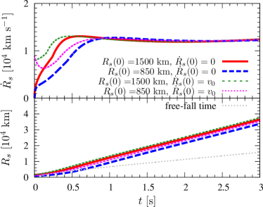
Figure 1: Time evolutions of shock velocity (top panel) and shock radius (bottom panel). Four different lines represent different initial conditions for the shock radius ($R_{s}(0)=850$ km or 1500 km) and shock velocity ($\dot{R}_{s}(0)=0$ or $v_{0}=\sqrt{GM_{c}/2R_{s}(0)}$). The grey dotted line in the bottom panel represents the free-fall time at each radius.

Figure 1 presents the time evolutions of shock radius and shock velocity for a constant luminosity of $L_{w}=10^{52}$ erg s^-1. Three boundary conditions are needed to solve Eq. (9) because it is a third order differential equation. We set $R_{s}$, $\dot{R}_{s}$, and $\ddot{R}_{s}$ at $t=0$. Figure 1 shows models with different initial conditions; models with different injection points $R_{s}(t=0)=1500$ km ($M_{c}=1.5M_{\odot}$; red thick-solid and green thin-dashed lines), and $R_{s}(0)=850$ km ($M_{c}=M_{\odot}$; blue thick-dashed and magenta thin-dotted lines), and models with different initial velocity $\dot{R}_{s}(0)=0$ (two thick lines) and $\dot{R}_{s}(0)=v_{0}\equiv\sqrt{GM_{c}/2R_{s}(0)}$ (two thin lines) that is velocity necessary to overwhelm ram pressure (see Maeda & Tominaga, 2009). We find that the dependence on the initial $\ddot{R}_{s}$, which is $0$ for all models shown in this figure, is very minor so that we do not show its dependence here. In these calculations, $M_{s}(t=0)=0$, i.e. the mass below $R_{s}(0)$ is assumed to be a compact object and does not contribute to the mass of the shell. The almost constant velocity is a consequence of the density structure, $\rho_{0}(r)\propto r^{-\beta}$, with $\beta\approx 2$. The grey dotted line in the bottom panel represents the free-fall time scale, $t_{\mathrm{ff}}=\sqrt{R_{s}^{3}/G(M_{c}+M_{s})}$, for the corresponding radius.

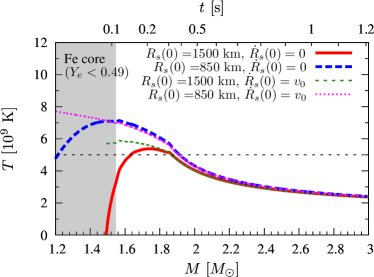
Figure 2: The postshock temperature as a function of mass coordinate. The model parameters are the same as in Figure 1. The horizontal dotted line represents $5\times 10^{9}$ K, above which ⁵⁶Ni is synthesized. The gray shaded region, $M(r)<1.55M_{\odot}$, is the iron core, where ⁵⁶Ni cannot be synthesized due to the low electron fraction of $Y_{e}<0.49$. The corresponding time of the model with $R_{s}(0)=850$ km and $\dot{R}_{s}(0)=v_{0}$ (magenta thin-dotted line) is given on the upper axis.

Figure 2 gives the temperature in the expanding shell as a function of mass coordinate for the same model as in Figure 1. The electron fraction in the iron core ($M\mathrel{\hbox{\hbox to0.0pt{\hbox{\lower 5.0pt\hbox{$\sim$}}\hss}\hbox{$<$}}}1.55M_{\odot}$) is less than 0.49 so that no ⁵⁶Ni production is expected. The maximum temperature of each mass element is determined by the energy injected until the shock front reaches the mass element. Thus, in order to achieve $T>5\times 10^{9}$ K just above the iron core, an initially fast shock wave or a shock injected deep inside is necessary. This is because smaller initial velocity leads to a smaller initial kinetic energy, and larger injection radius leads to shorter and smaller energy injection before the shock reaches a certain radius. We employ $R_{s}(0)=850$ km and $\dot{R}_{s}(0)=v_{0}$ to evaluate the maximum amount of ⁵⁶Ni in the following calculation. Although the model with $R_{s}(0)=850$ km and $\dot{R}_{s}(0)=0$ represents similar temperature, its expansion time of the shell is comparable to the free-fall time even for $L_{w}=10^{52}$ erg s^-1 (see Fig. 1), so that the explosion might fail.

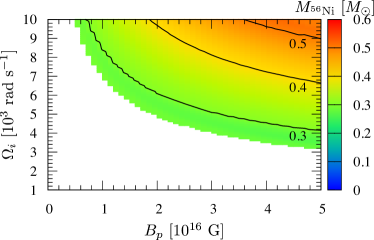
Figure 3: The amount of ⁵⁶Ni in units of $M_{\odot}$ for magnetar model as a function of the strength of the dipole magnetic field, $B_{p}$ and the initial angular velocity, $\Omega_{i}$. The region with $M<1.55M_{\odot}$ is not included because $Y_{e}<0.49$ and no ⁵⁶Ni production is expected there. Black solid lines represent $M_{{}^{56}\mathrm{Ni}}$ from 0.3 to 0.5 $M_{\odot}$.

Next, we consider the shock driven by the magnetar’s dipole radiation. Figure 3 shows the ⁵⁶Ni mass produced in the expanding shell as a function of $B_{p}$ and $\Omega_{i}$. In this figure, we employ $R_{\mathrm{NS}}=10$ km and $I=10^{45}$ g cm². Here, we assume that the matter that experienced $T>5\times 10^{9}$ K is completely converted to ⁵⁶Ni, i.e., $X(^{56}{\rm Ni})=1$, except for $M(r)<1.55M_{\odot}$ where $Y_{e}<0.49$. From this figure, we can easily see a rapid increase from 0 to $\sim$0.2$M_{\odot}$ of $M_{{}^{56}\mathrm{Ni}}$. In this progenitor, the silicon core has a mass of $\sim 1.84M_{\odot}$, and the density slope $\beta$ is different in the surrounding oxygen layer. This change in $\beta$ causes the change of velocity evolution shown in Figure 1: for instance, the blue thick-dashed line represents a rapid acceleration at $t\mathrel{\hbox{\hbox to0.0pt{\hbox{\lower 5.0pt\hbox{$\sim$}}\hss}\hbox{$<$}}}0.5$ s and a slow acceleration or an almost constant velocity afterwards.

Since the observed brightness of HNe requires $\sim 0.2$ – $0.5M_{\odot}$ of ⁵⁶Ni (Nomoto et al., 2006), a reasonable central engine model must achieve this quantity. We find that for $M_{{}^{56}\mathrm{Ni}}\mathrel{\hbox{\hbox to0.0pt{\hbox{\lower 5.0pt\hbox{$\sim$}}\hss}\hbox{$>$}}}0.2M_{\odot}$, the following relation should be satisfied;

$$\left(\frac{B_{p}}{10^{16~{}\mathrm{G}}}\right)^{1/2}\left(\frac{\Omega_{i}}{10^{4}~{}\mathrm{rad~{}s^{-1}}}\right)\mathrel{\hbox{\hbox to0.0pt{\hbox{\lower 5.0pt\hbox{$\sim$}}\hss}\hbox{$>$}}}0.68.$$ (15)

This condition can be derived by $E_{\mathrm{NS}}/T_{d}\mathrel{\hbox{\hbox to0.0pt{\hbox{\lower 5.0pt\hbox{$\sim$}}\hss}\hbox{$>$}}}5.3\times 10^{50}$ erg s^-1 (see Eqs. 4 and 5). Note that Eq. (15) is a conservative constraint because in this calculation we made several approximations, which always result in larger $M_{{}^{56}\mathrm{Ni}}$. Thus, for a more realistic case, $M_{{}^{56}\mathrm{Ni}}$ becomes smaller than this estimate. To make a reasonable amount of ⁵⁶Ni to explain the observation, a more energetic central engine is needed.

In order to investigate the progenitor dependence, we perform the same calculation with different progenitor models and find that the RHS of Eq. (15) is $\sim$0.64 – 0.90; 0.68 for 20 $M_{\odot}$, 0.90 for 40 $M_{\odot}$, 0.64 for 80 $M_{\odot}$ models of Woosley & Heger (2007), and 0.71 for 20 $M_{\odot}$ model of Umeda & Nomoto (2005). Therefore, this criterion does not strongly depend on the detail of the progenitor structure. These calculations are performed with $M_{c}=M_{\odot}$ and $\dot{R}_{s}(0)=v_{0}$.

4 Summary and discussion

In this study, we employed the thin shell approximation for shock structure and calculated evolution of a shock wave driven by wind from a rapidly rotating neutron star with strong magnetic fields (“magnetar”). By evaluating temperature evolution that is consistent with the shock evolution, we obtained a constraint on the magnetar parameters, namely magnetic field strength and rotation velocity (see Eq. 15), for synthesizing enough amount of ⁵⁶Ni to explain brightness of HNe.

In this calculation, we employed several assumptions.

• The dipole radiation is dissipated between the NS and the shock and thermal pressure drives the shock evolution. This assumption leads to larger amount of ⁵⁶Ni than more realistic situations because if the conversion from Poynting flux to thermal energy is insufficient, the internal energy is smaller and the temperature in the shell is lower than the current evaluation. Therefore, the mass that experienced $T>5\times 10^{9}$ becomes smaller.

• The shock and energy deposition from the magnetar are spherical, which leads to larger ⁵⁶Ni mass. This is because fallback of matter onto a NS takes place and reduces $M_{{}^{56}\mathrm{Ni}}$, if the explosion energy is concentrated in a small region (Bucciantini et al., 2009; Maeda & Tominaga, 2009; Yoshida et al., 2014).

• All energy radiated by the NS is used for HN component, which is overestimated because a part of the energy should be used to make the relativistic jet component of a GRB.

• The density inside the shell is assumed to be the same as the progenitor model. This assumption results in the higher temperature and the larger $M_{{}^{56}\mathrm{Ni}}$ than realistic hydrodynamical calculations because the shock enhances not only the pressure but also the density in the shell.

• Matter which experiences $T>5\times 10^{9}$K consists only of ⁵⁶Ni, i.e. $X(^{56}\mathrm{Ni})=1$. This overestimates $M_{{}^{56}\mathrm{Ni}}$ because $X(^{56}\mathrm{Ni})<1$ even in the layer which experiences $T>5\times 10^{9}$ K according to hydrodynamical and nucleosynthesis simulations (Tominaga et al., 2007).

• The mass cut corresponds to the iron core mass, $1.55M_{\odot}$. If the NS mass is larger than the iron core mass, the ⁵⁶Ni mass becomes even smaller.

• The ram pressure is neglected in the evolutionary equation of the shell. According to the estimate of the shock propagation time and the free-fall time, in the low luminosity case the shell could not propagate outward for more realistic calculations.

Combining these facts, our estimation of the ⁵⁶Ni mass is probably highly overestimated so that our constraint on the magnetar parameters (Eq. 15) is rather conservative. Interestingly, it is still a stringent constraint; a very high magnetic field strength and a very rapid rotation are required to explain the brightness of HNe.

Next, we discuss about more detailed MHD simulations for mechanisms driving ejecta by transferring rotational energy of magnetars using magnetic fields, although the mechanism is different from dipole radiation assumed in this study. Bucciantini et al. (2009) performed MHD simulations around new-born magnetars from 1 s after supernova shock emergence and found that the energy extracted from magnetars through magnetic fields is confined in the jet (directed flow) and the temperature cannot be high enough to produce ⁵⁶Ni even for the most energetic model in their study ($B=3\times 10^{15}$ G and $\Omega\approx 6000$ rad s^-1). More recently, MHD simulations with detailed microphysics, which run from onset of iron-core collapse to the explosion driven by magnetic fields, showed that the resultant ⁵⁶Ni amount was $\mathrel{\hbox{\hbox to0.0pt{\hbox{\lower 5.0pt\hbox{$\sim$}}\hss}\hbox{$<$}}}0.04M_{\odot}$ (Nishimura et al., 2015) for model with $B\sim 10^{15}$ G and $\Omega\approx 3000$ rad s^-1 (found in Takiwaki et al., 2009, for hydrodynamic explanations of their models). Therefore, ⁵⁶Ni amount cannot be amplified even when we take into account such MHD driven outflow.

There have been some studies that tried to explain the plateau phase of the early afterglow by the magnetar scenario because the long lasting activity can be explained by long-living magnetars. This discriminates magnetar scenario from the collapsar scenario, whose lifetime is determined by the accretion timescale of the hyperaccretion flow. The typical values for $B_{p}$ and $\Omega_{i}$ for long GRBs are $\mathrel{\hbox{\hbox to0.0pt{\hbox{\lower 5.0pt\hbox{$\sim$}}\hss}\hbox{$>$}}}3\times 10^{14}$ G and $\mathrel{\hbox{\hbox to0.0pt{\hbox{\lower 5.0pt\hbox{$\sim$}}\hss}\hbox{$>$}}}6\times 10^{3}$ rad s^-1 (Troja et al., 2007) and 3.2 – 12$\times 10^{14}$ G and 1.7-6.3$\times 10^{3}$ rad s^-1 (Dall’Osso et al., 2011). These values are far less than those given by Eq. (15). Therefore, if these GRBs are actually driven by a magnetar, we cannot expect the bright emission of HNe generated by the decay of ⁵⁶Ni. When we observe a GRB accompanying a HN, whose early afterglow can be explained by a magnetar with not fulfilling the constraint given by Eq. (15), we need an additional energy source to synthesize ⁵⁶Ni other than the dipole radiation from magnetars.

Since the magnetar scenario was recently suggested for the central engine of superluminous supernovae (SLSNe) (e.g. Kasen & Bildsten, 2010; Woosley, 2010; Gal-Yam, 2012) as well as GRBs, our discussion is applicable to this class of explosion. For instance, Kasen & Bildsten (2010) proposed that $B_{p}\sim 5\times 10^{14}$ G and $\Omega_{i}\sim 10^{2}$ – $10^{3}$ rad s^-1 are required to power the light curve of SLSNe. Thus, if the magnetar powers SLSNe, the synthesis of ⁵⁶Ni, i.e., ⁵⁶Fe, is not expected. This is contrast to a pair-instability supernova that is an alternative model for SLSNe.

Appendix A Test calculations

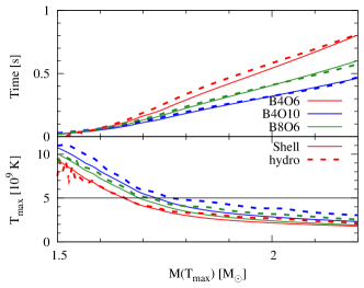
Figure 4: The passing time (top panel) and maximum temperature (bottom panel) for the shock as a function of mass coordinate. Solid and dotted curves represent the results of shell approximation (this work) and a hydrodynamic simulation, respectively. Colors represent magnetar parameters, $B=4\times 10^{16}$ G and $\Omega_{i}=6000$ rad s^-1 (red), $B=4\times 10^{16}$ G and $\Omega_{i}=10^{4}$ rad s^-1 (blue), and $B=8\times 10^{16}$ G and $\Omega_{i}=6000$ rad s^-1 (green). The horizontal dashed line in the bottom panel represents the critical temperature for ⁵⁶Ni synthesis, $5\times 10^{9}$ K.

Here, we show the validity of our calculation by comparing our calculation with a hydrodynamic simulation. In this comparison, we employ magnetars with three different sets of $B$ and $\Omega_{i}$, injected at $M(r)=1.45M_{\odot}$ of the 20$M_{\odot}$ progenitor of Umeda & Nomoto (2005). In Figure 4, we show the comparison of the passing time (top panel) and the maximum temperature (bottom panel) as a function of mass coordinate for the shell calculation and the hydrodynamic simulation (Tominaga et al., 2007). The shock and temperature evolutions computed with these different methods agree quite well and the systematic error of our thin shell approximation for ⁵⁶Ni mass is $\sim O(0.01)M_{\odot}$, which is smaller than the characteristic amount of ⁵⁶Ni of HNe, $O(0.1)M_{\odot}$.

References

- Blinnikov et al. (2000) Blinnikov S., Lundqvist P., Bartunov O., Nomoto K., Iwamoto K., 2000, ApJ, 532, 1132
- Bucciantini et al. (2009) Bucciantini N., Quataert E., Metzger B. D., Thompson T. A., Arons J., Del Zanna L., 2009, MNRAS, 396, 2038
- Burrows et al. (2007) Burrows A., Dessart L., Livne E., Ott C. D., Murphy J., 2007, ApJ, 664, 416
- Dall’Osso et al. (2011) Dall’Osso S., Stratta G., Guetta D., Covino S., De Cesare G., Stella L., 2011, A&A, 526, A121
- Dessart et al. (2008) Dessart L., Burrows A., Livne E., Ott C. D., 2008, ApJ, 673, L43
- Freiburghaus et al. (1999) Freiburghaus C., Rembges J.-F., Rauscher T., et al., 1999, ApJ, 516, 381
- Gal-Yam (2012) Gal-Yam A., 2012, Science, 337, 927
- Hjorth & Bloom (2012) Hjorth J., Bloom J. S., 2012, The Gamma-Ray Burst - Supernova Connection, 169–190
- Kasen & Bildsten (2010) Kasen D., Bildsten L., 2010, ApJ, 717, 245
- Komissarov & Barkov (2007) Komissarov S. S., Barkov M. V., 2007, MNRAS, 382, 1029
- Koo & McKee (1990) Koo B.-C., McKee C. F., 1990, ApJ, 354, 513
- Laumbach & Probstein (1969) Laumbach D. D., Probstein R. F., 1969, Journal of Fluid Mechanics, 35, 53
- LeBlanc & Wilson (1970) LeBlanc J. M., Wilson J. R., 1970, ApJ, 161, 541
- MacFadyen & Woosley (1999) MacFadyen A. I., Woosley S. E., 1999, ApJ, 524, 262
- Maeda et al. (2002) Maeda K., Nakamura T., Nomoto K., Mazzali P. A., Patat F., Hachisu I., 2002, ApJ, 565, 405
- Maeda & Tominaga (2009) Maeda K., Tominaga N., 2009, MNRAS, 394, 1317
- Meier et al. (1976) Meier D. L., Epstein R. I., Arnett W. D., Schramm D. N., 1976, ApJ, 204, 869
- Metzger et al. (2011) Metzger B. D., Giannios D., Thompson T. A., Bucciantini N., Quataert E., 2011, MNRAS, 413, 2031
- Mösta et al. (2014) Mösta P., Richers S., Ott C. D., et al., 2014, ApJ, 785, L29
- Nagataki et al. (2006) Nagataki S., Mizuta A., Sato K., 2006, ApJ, 647, 1255
- Nakamura et al. (2001a) Nakamura T., Mazzali P. A., Nomoto K., Iwamoto K., 2001a, ApJ, 550, 991
- Nakamura et al. (2001b) Nakamura T., Umeda H., Iwamoto K., et al., 2001b, ApJ, 555, 880
- Nishimura et al. (2015) Nishimura, N., Takiwaki, T., & Thielemann, F.-K. 2015, arXiv:1501.06567
- Nomoto et al. (2006) Nomoto K., Tominaga N., Tanaka M., et al., 2006, Nuovo Cimento B Serie, 121, 1207
- Sawai et al. (2013) Sawai H., Yamada S., Suzuki H., 2013, ApJ, 770, L19
- Shapiro & Teukolsky (1983) Shapiro S. L., Teukolsky S. A., 1983, Black holes, white dwarfs, and neutron stars: The physics of compact objects, New York, Wiley-Interscience, 1983, 663 p.
- Symbalisty (1984) Symbalisty E. M. D., 1984, ApJ, 285, 729
- Takiwaki et al. (2009) Takiwaki T., Kotake K., Sato K., 2009, ApJ, 691, 1360
- Thompson et al. (2004) Thompson T. A., Chang P., Quataert E., 2004, ApJ, 611, 380
- Tominaga (2009) Tominaga N., 2009, ApJ, 690, 526
- Tominaga et al. (2007) Tominaga N., Maeda K., Umeda H., et al., 2007, ApJ, 657, L77
- Troja et al. (2007) Troja E., Cusumano G., O’Brien P. T., et al., 2007, ApJ, 665, 599
- Umeda & Nomoto (2005) Umeda H., Nomoto K., 2005, ApJ, 619, 427
- Usov (1992) Usov V. V., 1992, Nature, 357, 472
- Whitworth & Francis (2002) Whitworth A. P., Francis N., 2002, MNRAS, 329, 641
- Winteler et al. (2012) Winteler C., Käppeli R., Perego A., et al., 2012, ApJ, 750, L22
- Woosley (1993) Woosley S. E., 1993, ApJ, 405, 273
- Woosley (2010) Woosley S. E., 2010, ApJ, 719, L204
- Woosley & Bloom (2006) Woosley S. E., Bloom J. S., 2006, ARA&A, 44, 507
- Woosley & Heger (2007) Woosley S. E., Heger A., 2007, Phys. Rep., 442, 269
- Woosley et al. (2002) Woosley S. E., Heger A., Weaver T. A., 2002, Reviews of Modern Physics, 74, 1015
- Yoshida et al. (2014) Yoshida T., Okita S., Umeda H., 2014, MNRAS, 438, 3119