Stochastic Modeling and Simulation of Ion Transport through Channels

Abstract

Ion channels are of major interest and form an area of intensive research in the fields of biophysics and medicine since they control many vital physiological functions. The aim of this work is on one hand to propose a fully stochastic and discrete model describing the main characteristics of a multiple channel system. The movement of the ions is coupled, as usual, with a Poisson equation for the electrical field; we have considered, in addition, the influence of exclusion forces. On the other hand, we have discussed about the nondimensionalization of the stochastic system by using real physical parameters, all supported by numerical simulations. The specific features of both cases of micro- and nanochannels have been taken in due consideration with particular attention to the latter case in order to show that it is necessary to consider a discrete and stochastic model for ions movement inside the channels.

1 Introduction

Ion channels are of major interest and form an area of intensive research in the fields of biophysics and medicine, since they control many vital physiological functions. Since certain aspects of ion channel structure and function are hard or impossible to address in real experiments, mathematical models form a useful addition, support and possible guidelines for future investigations.

Ion channels are membrane proteins that catalyze the transfer of ions down their electrochemical gradients across the plasma membrane [33]. They cannot perform thermodynamic work; that is, they are not able to move an ion against its electrochemical gradient. As a consequence, the direction of ions traveling through an open channel is solely dependent on the electrochemical gradient. Another characteristic of ion channels is that the rate at which ions move through these proteins is very high; the throughput of an ion channel can be fast up to 100 million ions per second [33]. On a fundamental level, the activity of ion channels can change the membrane potential of the cell or alter the concentrations of ions inside the cell. These processes are basic to the cell physiology; therefore, it is easily imagined that ion channels may be involved, directly or indirectly, in virtually all cellular activities. While the role of some ion channels is known, as for example for calcium or sodium channels, in other cases the physiological role of an ion channel is unknown, and sometimes it is discovered when a disease arises.

We are aware of the need of analyzing many more features of a system of ion channels, so that the model presented here is not meant to be an exhaustive description of all relevant phenomena which enter the dynamical behavior of ion channels. Though, it can be seen as a first step anticipating more complex, hence more realistic, models.

A summary of the main features of ion channel mechanism is the following [33, 44]:

a. The electrochemical gradient: This determines the direction along which ions will flow through an open ion channel and is a combination of two types of gradients: a concentration gradient and an electrical field gradient. The electrical field gradient takes into account the charge on the ion. The relationship between the electrical potential and the magnitude of the concentration gradient that is created is intuitive: the stronger the electrical potential, the greater the concentration gradient.

b. The current-voltage relationship: The current is given by the movement of charges, and in cells the flow of ions through ion channels can be measured.

c. The anatomy of a typical ion channel: The ion channels are proteins with a hole in their middle Their walls contain ionizable side chains producing high charge densities [11, 14, 15].

d. The ion selectivity: The capacity of the membrane to be permeable to a class of ions. The mechanism by which ion channels pick and choose certain ions is still not fully understood. Selectivity is produced by physical forces that depend on the ion charge and size and chemical interactions with parts of the channel protein that form what is called the selectivity filter [14, 15].

e. The ion gating: The opening and closing mechanism of ion channels.

f. The solvent: Ions move in water; hence a realistic model should eventually include the fluid dynamics of the system.

In the present work we shall essentially consider only the movement of ions subject to ion-ion interactions, interaction with the geometry of the channels, and the coupling with the electrical field which fluctuates, due to the strong interaction with ions themselves. By taking all this into account, we have already achieved a high level of complexity of the system. It is clear that further steps will be in the direction of including the selectivity and gating processes, which are essentials in the channel dynamics. Selectivity and gating are also influenced by the enormous densities of fixed charges since channels are small and walls contain ionizable side chains and carbonyl oxygens which produce an effective charge density [14, 15]. As mentioned later on, we do not enter into such a level of description, that may be included in the modeling later on; here we consider a mathematical schematization of the walls of the channels with which ions interact via specific potentials. Furthermore, here solvent effects enter through the dielectric and the diffusion coefficients only, but a more complete model should also include a mathematical description of the solvent water. A proposed model may be found in [13], where the authors couple a continuum model for the ion density with a Navier–Stokes system for the water treated as an incompressible fluid. It is also clear that salt water contains many families of particles, as sodium, potassium, calcium, and chloride ions with different physical characteristics, as, for example, different diameters. For the sake of simplicity, here we study the dynamics of a single family of ions, i.e. the diameter of ions is the same for all.

There is widespread literature on molecular dynamics simulation methodology for studying ionic permeation in ion channels, where authors use fully atomistic simulations of the entire systems. The reader may refer, for example, to [1, 7, 8, 11, 18, 22, 23, 27, 29, 32, 37]. However, Brownian dynamics may represent an attractive computational approach for simulating the permeation process through ion channels over long time-scales without having to treat a system in all atomic details explicitly. The approach consists of the generation of random trajectories of ions as a function of time, by numerically integrating stochastic equations for the motion using some effective potential function to calculate the microscopic forces operating among them [18, 23]. This reduces the dimensionality of the problem, although already very high, making BD less computationally intensive than the corresponding molecular dynamics simulations. While various approaches for microscopic modeling, either based on equations for the motion with forces accounting for finite sizes [9, 10, 27, 28] or on exclusion processes, have been investigated in detail, there are still open problems in the transition to macroscopic models based on partial differential equations. Some recent literature involves some heuristic derivations of macroscopic dynamics [2, 30, 41]. Often away from equilibrium standard equations with linear terms are used, whose appropriateness remains unclear. In order to model some exclusion principle, in [2] the following modified Poisson–Nernst–Planck equations have been obtained via a heuristic derivation from an exclusion discrete process;

$$-\epsilon\Delta V = e\left(\sum_{j}z_{j}c_{j}+f\right)$$

$$\frac{\partial}{\partial t}c_{i} = \nabla\cdot\left(D_{i}(1-\rho)\nabla c_{i}+c_{i}\nabla\rho+ez_{i}\mu_{i}c_{i}(1-\rho)\nabla V\right))$$

where $c_{i}$ is the concentration , $z_{i}$ the charge, $D_{i}$ the diffusion coefficient, and $\mu_{i}$ the mobility of the ions of type $i$; $\rho=\sum_{i}c_{i}$ is the total concentration, $V$ the electrical potential, $\epsilon$ the permittivity, and $e$ the elementary charge. Hence, the authors introduce a size exclusion effect. The derivation of the continuum model is not completely rigorous, so there still is a lot of work that needs to be done in such a direction. A different approach used to deal with the finite size of particle is via a Fermi like distribution, as in [20].

As mentioned in [29, 30, 31] while macroscopic conservation laws clearly govern the macroscopic behavior of ensembles of channels, their application to a single protein channel able to contain at most one or two ions is questionable. The same authors in [41] consider a stochastic treatment of the ions. Their aim is a reduction of the complexity of solving the multidimensional Fokker–Planck system associated with the stochastic Langevin system of all ions, coupled with the Poisson equation for the electrical potential associated with all ions. They perform their analysis upon the assumption of stationary joint probability density of all ions, and under the additional simplification that positive ions of the same species are indistinguishable and interchangeable. Finally, they decoupled position and velocity by considering the Smoluchowski limit of large friction. Among the problems that are left open, they mention the size exclusion effect of ions and the multiple channel case. Here we propose a first attempt in this direction.

The aim of the present work is, first of all, to consider a fully stochastic model able to describe the main characteristics of a multiple channel system, in which ion movement in the bath and throughout channels is described via a system of stochastic differential equations, coupled with a Poisson equation, which becomes itself stochastic due to the dependence upon the ion random positions. The treatment of multichannel systems becomes important in the description when the number of channels increases. In such living devices, ions are not points and cannot overlap; as a consequence, atomic scale distances must be included explicitly in this multiscale approach [14, 17]. Hence, exclusion forces are considered and modeled via Pauling and Lennard–Jones potentials. Pauling forces take into account the interaction among ions, while Lennard–Jones potential takes into account the interaction of moving ions with the boundary of the channels, in particular their reflection at the channels’ boundary. One of the main problems so widespread in literature [2, 7, 12, 25, 29, 30, 31] has been to link such a completely stochastic model with an averaged continuum model described by partial differential equations. Actually it is well known that it becomes reasonable to consider a continuous model when laws of large numbers may be applied [3, 4, 5], i.e. when the number of ions increases to infinity or the population is large enough that an approximation may be applied. It is clear that, while this is always the case in the bath, this is not always true in the channels; indeed, as already mentioned, in the specific case of nanochannels the dimension of the ions is of the same order as the one of a channel, so that in a channel the description of the system has to remain discrete and stochastic. As a consequence, in the limit of infinite (sufficiently large) number of ions, a problem of coupling their dynamics outside (averaged continuum) and inside (discrete stochastic) channels arises. We may refer to such a model as a hybrid model, as in [26]. The present work means to be a first step in this direction; via a simulation analysis we build up a discrete stochastic model and understand the role of each parameter. As also mentioned in [17], some systems have macroscopic effects that depend on atomic details. Indeed, at a later stage our plan is to analyze the asymptotic behavior of the system as the number of ions increases to infinity or typical parameters characterizing the system, as e.g. the size pore, vanish to zero. In literature we may see a widespread interest on the latter topic, but most of the results refer to averaging problems of continuum deterministic Poisson–Nernst–Planck equations [39, 40]. The treatment of a fully stochastic case is still open.

Here the issue of nondimensionalization of the stochastic system and the choice of the right space-time rescaling to catch the main features of the dynamics has been addressed. Since we have many parameters, we discuss also how we may standardize some of them, and the role played by the others. Even though the issue of nondimensionalization is very well known in literature [2], the best of our knowledge there is no such explicit calculation, analysis, or similar discussion. The proposed space rescaling is strictly related to the size of the channels and of the ions, while the time rescaling depends on the possibility to treat the stochastic part of the Langevin equation, described by the Wiener process. We discuss the role of different rescalings by comparing the outcome of the dynamics obtained by numerical simulations. In particular, we compare two different rescalings by referring to specific length measures of the channels. Both cases of micro- and nanochannels are considered.

2 The Model

We consider a domain $\Omega=\Omega_{+}\cup\Omega_{-}\cup\Omega_{M}\in\mathbb{R}^{d},$ which consists of two regions of intra- and extra-cellular medium, $\Omega_{+}$ and $\Omega_{-}$, divided by the membrane domain $\Omega_{M}$, composed of many similar channels; let us denote by $\Gamma_{D_{+}}$ and $\Gamma_{D^{-}}$ the superior and inferior boundary of the bath, respectively. Typically, for a proper match with the biological case, we consider $d=3$, while in order to reduce the complexity of the study, the simulation domain is such that $d=2$.

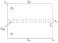
Figure 1: Computational domain in $\mathbb{R}^{2}$, di dimension $L_{1}\times L_{2}$ with dimension of the membrane $\epsilon_{2}\times L_{1}$.

We suppose that the membrane has dimension $L_{1}\times L_{1}\times\epsilon_{2}\in\mathbb{R}^{3}$; the dimension of each pore is $\epsilon_{1}\times\epsilon_{1}\times\epsilon_{2}\in\mathbb{R}^{3}$; hence, in the membrane we have $\lfloor L_{1}/2\epsilon_{1}\rfloor\in\mathbb{N}$ pores. So we have sketched each channel as a three-dimensional parallelepiped with typical dimensions $\epsilon_{1}$ and $\epsilon_{2}$ ( $\epsilon_{1}<\epsilon_{2}$). See Figure 1 for the two-dimensional case.

Ions move freely in the water, which is treated as a continuum, and their motion through channels is driven by an electrical field, described as a gradient of an electrical potential.

We need to describe the ions, their dynamics, the electrical field, and the reciprocal interactions.

2.1 The Variables

The Ions. In general, we might suppose that $K\in\mathbb{N}$ is the total number of types of ions; out of them, the first $K-1$ are free species and the $K$th is a species confined in the membrane region, which creates the permanent charge of the channels. As a consequence, in the domain we have a number $N+J=\sum_{k=1}^{K-1}N^{k}+J$ of ions, where $N^{k}$ is the number of ions of the $k$th species and $J$ the number of fixed confined ions. The first $N$ ions are moving in $\Omega$ and each of them is characterized by its Langevin coordinates, i.e. $\left(X^{k,j}(t),V^{k,j}(t)\right)\in\Omega\times\mathbb{R}^{3}$, being, respectively, the location and the velocity of the $j$th ion, of the $k$th species, with $j=1,\ldots,N^{k}(t)$. The latter $J$ fixed charges are characterized by their position $Y^{j}\in\Omega_{M},j=1,\ldots,J.$

Here we consider a simplified model with $K=2$, that is the case where only one population of ions is free of moving in $\Omega$ and the other one is composed by fixed charges, few in number, located in the upper region of the channels [21].

Hence, let $N$ be the total number of moving ions in the domain $\Omega\subset\mathbb{R}^{3}$. Each ion is characterized by its Langevin coordinates, i.e.

$$Z^{j}=\left(X^{j},V^{j}\right)\in\Omega\times\mathbb{R}^{3},\quad j=1,\ldots,N,$$

being, respectively the location and the velocity of the $j$th ion out of $N$. Furthermore, let $Y^{j},j=1,\ldots,J$ be the position of the $j$th fixed charge out of $J$.

Each ion is also characterized by its occupied volume of order ${\tilde{\epsilon}}\,^{3}$, being $\tilde{\epsilon}$ its diameter. If $\tilde{\epsilon}\sim\epsilon_{1}$, we are in the case of nanochannels, i.e. a finite small number of ions may enter each channel, while if $\tilde{\epsilon}\ll\epsilon_{1}$, we are in the case of microchannels.

We consider the following counting measure defined on the location-velocity space $\Omega\times\mathbb{R}^{3}$

$$\mu_{Z}(t) = \sum_{j=1}^{N}\epsilon_{Z^{j}(t)}=\sum_{j=1}^{N}\epsilon_{(X^{j}(t),V^{j}(t))}\in\mathcal{M}{(\Omega\times\mathbb{R}^{3})},$$ (1)

$$\nu_{Y} = \sum_{h=1}^{J}\epsilon_{Y^{h}}\in\mathcal{M}{(\Omega)}.$$ (2)

As a consequence, from (1), the moving ion spatial counting process is given by

$$\nu_{X}(t) = \mu_{Z}(t)(\cdot\times\mathbb{R}^{3})=\sum_{j=1}^{N}\epsilon_{X^{j}(t)}\in\mathcal{M}{(\Omega)}.$$ (3)

Finally, we may also consider the following empirical measures

$$X(t) = \frac{1}{N}\nu_{X}(t)\in\mathcal{M}_{P}{(\Omega)};$$ (4)

$$Y = \frac{1}{J}\nu_{Y}\in\mathcal{M}_{P}{(\Omega)}.$$ (5)

In (3)-(5) $\mathcal{M}{(\Omega)}$ and $\mathcal{M}_{P}{(\Omega)}$ denote the spaces of (discrete) measures and probability measures on $\Omega$, respectively.

The Electrical Field. The electrical field $E(t,x)$ (in $V/m$) is described by means of an electrical potential $\Phi(t,x)$ (in $V=kg\,m^{2}/s^{2}\,C$), which is a continuous variable on $\Omega_{T}=[0,T]\times\Omega$.

2.2 The Dynamics

A strong coupling between the variation of the distribution charges and the variation of the electrical potential is shown.

The Electrical Field. The electrical potential $\Phi$ is the solution of the Poisson equation

$$\begin{split}\textbf{}-\nabla\cdot\left(\alpha_{w}\nabla\Phi(t,x)\right)&=z\leavevmode\nobreak\ q\leavevmode\nobreak\ (K_{\kappa_{1}}*X(t))(x)+z_{F}\leavevmode\nobreak\ q\leavevmode\nobreak\ (K_{\kappa_{2}}*Y)(x),\end{split}$$ (6)

where $\alpha_{w}$ is the dielectric constant for the water (in $F/m=C/Vm$), $z$ is the valency of the free ions, $z_{F}$ is the valency of the fixed ions, and $q$ is the charge of ions (in $C$). The smoothing functions $K_{\kappa_{i}}\in C_{b}^{2}(\mathbb{R}^{3}),i=1,2$, are such that

$$K_{\kappa_{i}}(x)=\frac{1}{\kappa_{i}}U_{i}(x),\quad x\in\Omega,$$ (7)

where, for any $i=1,2$, the function $U_{i}\in C_{b}^{2}(\mathbb{R}^{3})$ has compact support equal to $\kappa_{i}$, i.e. $|\textrm{supp}(U_{i})|=\kappa_{i}$. In such a way, the quantities at the right-hand side of (6) has the right dimension of a concentration, i.e. quantity of charge per unit volume. Furthermore, the convolution terms in (6) may be seen as an empirical concentration, justifying the dependence on $N$, via the empirical measure $X(t)$, given by (4).

For any $t\in[0,T]$, the boundary conditions are given by

$$\begin{split}\Phi(t,x)&=\Phi_{1},\quad x\in\Gamma_{D^{+}};\\ \Phi(t,x)&=\Phi_{2},\quad x\in\Gamma_{D^{-}};\\ \frac{\partial\Phi(t,x)}{\partial\nu}&=0,\qquad x\in\partial\Omega\setminus(\Gamma_{D^{+}}\cup\Gamma_{D^{-}}).\end{split}$$ (8)

The Moving Ions. The $N\in\mathbb{N}$ free ions move in the surrounding water along a direction determined by the electrochemical gradient; they interact with each other and with the walls of the membrane. An external source of randomness is introduced in the acceleration field, so that the evolution of the ions state $Z^{j}(t)=(X^{j}(t),V^{j}(t))$, for $j=1,\ldots,N$ is described by the following Langevin model:

$$dX^{j}(t) = V^{j}(t)dt,$$ (9)

$$mdV^{j}(t) = -\left[m\leavevmode\nobreak\ \gamma V^{j}(t)+z\leavevmode\nobreak\ q\leavevmode\nobreak\ \nabla\Phi(t,X^{j}(t))\right.$$

$$\hskip 11.38092pt+F_{I}\nabla\left(H_{P}^{*}[\nu_{X}(t)+\nu_{Y}]\right)(X^{j}(t))$$

$$\hskip 11.38092pt\left.+F_{I}\nabla H_{LJ}(d_{\partial\Omega_{M}}(X^{j}(t))\right]\,dt+\sigma dW_{t}^{j}.$$

In System (9)-(2.2), $m$ is the effective mass of the ions (in $kg$), $\gamma$ is the friction coefficient per unit of mass (in $s^{-1}$), describing the effect of the surrounding water molecules; they are related to the diffusion coefficient $D$ (in $m^{2}/s$) deriving from random collisions with water as shown by the Stokes–Einstein relation [36]

$$m\gamma=\frac{K_{B}T}{D},$$ (11)

where $K_{B}$ is the Boltzmann constant ($1.30\cdot 10^{-23}J/K=1.30\cdot 10^{-23}kg\,m^{2}/s^{2}\,K$) and $T$ is the absolute temperature (in $K$).

The stochastic effect is described by a multivariate Wiener process $({W}^{1}_{t},\ldots,W_{t}^{N})_{t\geq 0}$ with independent components. The parameter $\sigma$ (in $kg\,m/s\sqrt{s}$) is the diffusion coefficient, acting upon $mV^{j}(t)$, for any $j=1,\ldots,N;$ it must satisfy the following relation with $\gamma$:

$$m\gamma=\frac{1}{2K_{B}T}\sigma^{2}=C_{KT}\sigma^{2}.$$ (12)

Finally, the constant $F_{I}$ (in $N$) represents the magnitude of short range forces at contact. One estimate is given in [27] and is of the order $10^{-10}N$.

In System (9)-(2.2) we also introduced an ion-ion interaction through the Pauling potential $H_{P}$. Following [27], we might consider

$$H_{P}(r)=\frac{(r_{1}+r_{2})^{10}}{9r^{9}}.$$ (13)

It represents a repulsive potential which arises from the overlap of the electron clouds of the ions, $r$ is the ion-ion distance, and $r_{i},i=1,2,$ are the van der Waals radii of ions. Here, since we consider only one single family of ions, $r_{1}=r_{2}$, we define the operator $H_{P}^{*}[\nu_{Z}(t)+\nu_{Y}](x)$ as the following:

$$H_{P}^{*}[\nu_{X}(t)+\nu_{Y}](x):=\sum_{k=1}^{N}H_{P}(|X^{k}(t)-x|)+\sum_{j=1}^{J}H_{P}(|Y^{j}-x|),$$ (14)

where $|x|$ is the norm of $x$ and $|x-y|$ denotes the distance between $x,y\in\mathbb{R}^{3}$, that is

$$|x-y|=\sqrt{\sum_{i=1}^{3}(x_{i}-y_{i})^{2}}.$$

The walls of the membrane are made of fixed particles of a repulsive nature with respect to the moving ions. A mathematical schematization to include the boundary conditions has been made via a hard-wall potential, like a truncated shifted Lennard–Jones potential activated when the ions are at fixed distance from the boundary [32, 19, 20, 34]. In (2.2) the quantity $d_{\partial\Omega_{M}}(x)$ denotes the distance of a point $x\in\Omega$ from the boundary of the membrane $\partial\Omega_{M}$, that is

$$d_{\partial\Omega_{M}}(x)=\min_{y\in\partial\Omega_{M}}\left|x-y\right|.$$ (15)

The truncated shifted Lennard–Jones potentials, as suggested in [32], has the following form:

$$H_{LJ}(r)=\left\{\begin{array}[]{ll}\widetilde{H}_{LJ}(r)-\widetilde{H}_{LJ}(r_{c}),&\hbox{ }r\leq r_{c};\\ 0,&\hbox{ }r>r_{c},\\ \end{array}\right.$$ (16)

where $r$ is the distance between two particles and $\widetilde{H}$ is the Lennard–Jones potential which includes attraction-repulsion effects

$$\widetilde{H}_{LJ}(r)=\varepsilon_{LJ}\left[\left(\frac{\tilde{\epsilon}}{r}\right)^{12}-2\left(\frac{\tilde{\epsilon}}{r}\right)^{6}\right].$$ (17)

In (17), $\varepsilon_{LJ}$ is the well depth (in $m$) and a measure of how strongly the two particles attract each other; $\tilde{\epsilon}$ is the distance at which the intermolecular potential between the two particles is zero; it gives a measurement of how close two nonbonding particles can get and is thus referred to as the van der Waals radius. Here we treat $\tilde{\epsilon}$ as the diameter of the ions, i.e. it is of same order of the van der Waals radius. Table 1 shows the size of some families of ions.

Ions	vdW radius
$Ca^{2+}$	$114\,\,pm$
$Na^{+}$	$116\,\,pm$
$K^{+}$	$152\,\,pm$
$Cl^{-}$	$167\,\,pm$

Table 1: Van der Waals radii $\widetilde{\epsilon}$ for some families of ions in picometers ($10^{-12}m$).

If we consider the truncated Lennard–Jones potential (16) with a cutoff $x_{c}=\tilde{\epsilon}$, only the repelling part of the potential $\widetilde{H}_{IJ}$ is taken into account; indeed,

$$\widetilde{H}_{LJ}\left(\tilde{\epsilon}\right)=-\varepsilon_{LJ},$$

and (16) becomes

$${H}_{LJ}(r) = \left(\widetilde{H}_{LJ}(r)+\varepsilon_{LJ}\right)1_{(0,\tilde{\epsilon}]}(r)$$

$$= -\varepsilon_{LJ}\left\{1-\left[\left(\frac{\tilde{\epsilon}}{r}\right)^{12}-2\left(\frac{\tilde{\epsilon}}{r}\right)^{6}\right]\right\}1_{(0,\tilde{\epsilon}]}(r).$$

The choice of $\varepsilon_{LJ}$ influences how much the potential $H_{LJ}$ tends to hard-sphere potential $H_{hs}$. For the truncated Lennard–Jones potential the choice $\varepsilon_{LJ}=1$ describes relatively “soft” molecules; that is, molecules can partially overlap during collisions, whereas if they are closer than $\tilde{\epsilon}$ they start to repel each other. By increasing $\varepsilon_{LJ}$, a hard-sphere behavior is mimicked.

Parameter	Value	Measure units
$q$	$1.6\times 10^{-19}$	$C$
$m$	$6.5\times 10^{-26}$	$Kg$
$D$	$1.33\times 10^{-9}$	$m^{2}\;s^{-1}$
$\epsilon_{1},\epsilon_{2}$	$10^{-9}-10^{-7}$	$m$
$F_{I}$	$2\times 10^{-10}$	$N$
$K_{B}$	$1.38\times 10^{-23}$	$J\;K^{-1}$
$T$	$300$	$K$
$\alpha_{w}$	$7.08\times 10^{-10}$	$C\;V^{-1}\;m^{-1}$
$\alpha_{0}$	$8.85\times 10^{-12}$	$C\;V^{-1}\;m^{-1}$

Table 2: List of the parameters used in the model. For the one related to ions, refer to the case of $K^{+}$.

In Table 2 the value of the model parameters is listed, in the case of $K^{+}$. We observe that their order of magnitude may be very different; in particular, mass $m\sim O(10^{-26}),$ while the friction term $m\gamma\sim O(10^{-12}),$ the charge $q\sim O(10^{-19})$, and the interaction $\sim O(10^{-10})$.

It is clear that in order to better manage System (6) and (9)-(2.2), a nondimensionalization procedure is needed.

3 Nondimensionalization of the system

We consider the nondimensionalization starting with a time-space rescaling, via some typical scale parameters $(t_{0},\epsilon)$.

3.1 Time, Space, positions, and Velocities

Let $(x_{s},t_{s})$ be the scaled space-temporal coordinates, such that

$$t=t_{0}\leavevmode\nobreak\ t_{s}\qquad x=\epsilon\leavevmode\nobreak\ x_{s},$$ (19)

where $\epsilon\in\mathbb{R}$ and $t_{0}\in\mathbb{R}_{+}$ are scaling parameters that will be chosen later on. As a consequence of (19) the time dependent position and velocity are scaled as follows:

$$\begin{split}x_{s}(t_{s})&=\epsilon^{-1}x(t_{0}^{-1}t)\\ v_{s}(t_{s})&=\frac{t_{0}}{\epsilon}v(t_{0}^{-1}t).\end{split}$$ (20)

We denote by $\Omega^{s}=\Omega^{s}_{+}\cup\Omega^{s}_{-}\cup\Omega^{s}_{M}$ the rescaled domain with the three different regions, and by $\Gamma^{s}_{D^{+}},\Gamma^{s}_{D^{-}}$ the superior and inferior boundary of the rescaled bath, respectively.

Given the Langevin coordinate of the moving ions at time $t_{s}$, for $j=1,\ldots,N,$

$$Z_{s}^{j}(t_{s})=\left(X_{s}^{j}(t_{s}),V_{s}^{j}(t_{s})\right)\in\Omega^{s}\times\mathbb{R}^{3},$$

and the position of the fixed ones $Y_{s}^{i}$, $i=1,\dots,J$, let us denote by $\nu_{X}^{s}(t_{s}),\nu_{Y}^{s},$ the corresponding counting processes at time $t_{s}$, that is

$$\nu_{X}^{s}(t_{s})={\displaystyle\sum_{j=1}^{N}\varepsilon_{X_{s}^{j}(t_{s})}},\qquad\nu_{Y}^{s}={\displaystyle\sum_{i=1}^{J}\varepsilon_{Y_{s}^{i}}},$$

and by $X^{s}(t_{s}),Y^{s}$ the corresponding empirical measures

$$X^{s}(t_{s})=\frac{1}{N}\nu_{X}^{s}(t_{s}),\qquad Y^{s}=\frac{1}{J}\nu_{Y}^{s}.$$

3.2 The Electrical Field

One might obtain a dimensionless equation for the potential $\Phi$ in several ways. Scaling the electrical potential means finding a scaling parameter $\widetilde{\Phi}$ such that the potential field $\Phi_{s}(t_{s},x_{s})$ in the new coordinates is

$$\Phi_{s}(t_{s},x_{s})=\frac{1}{\widetilde{\Phi}}\Phi(t_{0}t_{s},\epsilon x_{s}).$$ (21)

Proper techniques of semiconductor literature can be used for ion channels [16, 25]. Indeed, being ion channels provided of few fixed charges inside the channels, the applied difference of potential is approximately close to the thermal voltage. This fact represents a bridge between ion channels literature and the studies of semiconductors [38]. A way to rescale $\Phi$ is the following:

$$\widetilde{\Phi}=\frac{K_{B}T}{q}\approx 0.39\;J/C.$$

If the variation of $\Phi$ is smaller than ${K_{B}T}/{q}$, the diffusion prevails, otherwise the advection dominates. The chosen scaling corresponds to a limit in which both advection and diffusion are in balance.

3.3 Rescaling the Equations

We will consider a nondimensionalization of (6) and (9)-(2.2), based on the transformation proposed in (20)-(21). Details of the nondimensionalization may be found in the appendix.

The Poisson Equation

The scaled Poisson equation is

$$\begin{split}-\textrm{div}_{x_{s}}{\left(\alpha_{s}\nabla_{x_{s}}\Phi_{s}\left(t_{s},x_{s}\right)\right)}&=\lambda^{\epsilon}z\left(K_{\kappa_{1}^{s}}^{s}*X^{s}(t_{s})\right)(x_{s})+\lambda^{\epsilon}z_{F}\left(K_{\kappa_{2}^{s}}^{s}*Y^{s}\right)(x_{s}).\end{split}$$ (22)

In (22), the kernels $K_{\kappa_{i}^{s}},i=1,2$ have been scaled as follows:

$$K_{\kappa_{i}^{s}}(x_{s})=\frac{1}{\kappa_{i}^{s}}U_{i}^{s}(x_{s})=\frac{1}{\kappa_{i}^{s}}U_{i}\left(\epsilon x_{s}\right),$$ (23)

and the relative electrical permittivity $\alpha_{s}$ is such that

$$\alpha_{w}=\alpha_{s}\alpha_{0},$$ (24)

where $\alpha_{w}$ is the typical electrical permittivity of the water, and $\alpha_{0}$ is the electrical permittivity of the free space. For any $i=1,2$, the parameter $\kappa_{i}^{s}$ is obtained by the rescaling of the support $\kappa_{i}$ of $U_{i}$, that is $\kappa_{i}=\epsilon^{3}\kappa_{i}^{s}.$ See, again, Table 2 for their physical dimensions.

Finally, the parameter $\lambda^{\epsilon}$ is given by

$$\lambda^{\epsilon}=\dfrac{q}{\alpha_{0}\tilde{\Phi}\epsilon}=\dfrac{q^{2}}{\alpha_{0}K_{B}T}\frac{1}{\epsilon}.$$ (25)

Hence, it depends on the scaling length $\epsilon$. Note that, coherently with our purpose, the coefficient $\lambda^{\epsilon}$ is dimensionless, in fact we have

$$\dfrac{C^{2}}{\dfrac{C^{2}}{m\cdot J}\;JK^{-1}\;K\;m}=1.$$ (26)

Consistently with (21), in the new reference scale the boundary conditions (8) become

$$\begin{split}\Phi_{s}(t_{s},x_{s})&=\dfrac{\Phi_{1}}{\tilde{\Phi}}=\dfrac{q}{K_{B}T}\Phi_{1}=\Phi_{1,s},\qquad x_{s}\in\Gamma^{s}_{D^{+}};\\ \Phi_{s}(t_{s},x_{s})&=\dfrac{\Phi_{2}}{\tilde{\Phi}}=\dfrac{q}{K_{B}T}\Phi_{2}=\Phi_{2,s},\qquad x_{s}\in\Gamma_{D^{-}}^{s};\\ \dfrac{\partial\Phi_{s}}{\partial\nu}(t_{s},x_{s})&=0,\qquad x_{s}\in\partial\Omega_{M,s}\setminus(\Gamma_{D^{+}}^{s}\cup\Gamma_{D^{-}}^{s}).\end{split}$$ (27)

The Langevin system

The nondimensionalized Langevin system is, for any $j=1,\ldots,N$,

$$dX_{s}^{j}\left(t_{s}\right) = V_{s}^{j}\left(t_{s}\right)dt_{s},$$ (28)

$$m_{s}dV_{s}^{j}\left(t_{t_{s}}\right) = -\left[\lambda_{1}m_{s}\gamma_{s}V_{s}^{j}\left(t_{s}\right)\right.+\lambda_{2}\nabla_{x_{s}}\Phi_{s}\left(t_{s},X_{s}^{j}(t_{s})\right)$$

$$\hskip 8.5359pt\left.+\lambda_{3}\nabla_{x_{s}}{H_{P}^{s,*}}\left[\nu_{X}^{s}(t_{s})+\nu_{Y}^{s}\right](X_{s}^{j}(t_{s}))\right.$$

$$\hskip 8.5359pt\left.+\lambda_{3}\nabla_{x_{s}}H_{LJ}^{s}\left(d_{\partial{\Omega_{M}^{s}}}(X_{s}^{j}(t_{s}))\right)\right]dt_{s}$$

$$+\lambda_{4}\sigma_{s}dW_{t_{s}}.$$

In the previous system $m_{s},\sigma_{s}$, and $\gamma_{s}$ are such that $\gamma=\bar{\gamma}\gamma_{s},\sigma=\sigma_{s}\bar{\sigma},m=Mm_{s},$ and

$$\sigma_{s}=\sqrt{2m_{s}\gamma_{s}},\quad\bar{\sigma}=\sqrt{K_{B}TM\bar{\gamma}}.$$ (30)

The functions $H_{P}^{s},H_{LJ}^{s}$ are the scaled Pauling and Lennard–Jones potential

$$\widetilde{H}_{LJ}^{s}\left(x_{s}\right) = \varepsilon_{LJ}^{s}\left[\left(\dfrac{2R^{s}_{vdW}}{x_{s}}\right)^{12}-2\left(\dfrac{2R^{s}_{vdW}}{x_{s}}\right)^{6}\right],$$ (31)

$$H^{s}_{P}\left(r_{s}\right) = \dfrac{\left(r_{1,s}+r_{2,s}\right)^{10}}{r_{s}^{9}}.$$ (32)

Finally, the dimensionless coefficients $\lambda_{i},i=1,\dots,4$ in the Langevin system are

$$\lambda_{1}=t_{0}\bar{\gamma},\qquad\lambda_{2}=\dfrac{t_{0}^{2}K_{B}T}{M\epsilon^{2}},\qquad\lambda_{3}=\dfrac{F_{I}}{M}\dfrac{t_{0}^{2}}{\epsilon},\qquad\lambda_{4}=\dfrac{t_{0}\sqrt{t_{0}}}{M\epsilon}\sqrt{K_{B}TM\bar{\gamma}}.$$ (33)

So the nondimensionalized system has five parameters (25) and (33), depending on the time and space characteristic lengths $t_{0}$ and $\epsilon$.

3.4 Reduction of the Parameters

In order to reduce the parameters, first of all we impose $\bar{\gamma}=t_{0}^{-1}$, so that also $\lambda_{1}=1$. Furthermore, we choose the scaling parameter $t_{0}$ such that the random term is a Wiener process with diffusion coefficient $\sigma_{s}$; this is equivalent imposing that is $\lambda_{4}=1$. It follows that

$$t_{0}=\epsilon\sqrt{\dfrac{M}{K_{B}T}};$$ (34)

as a consequence, $\lambda_{2}=1.$ Hence, by (34), we have standardized three of the five parameters.

In conclusion, the nondimenzionalized system is given by the Poisson equation (22)-(25) and the following Langevin system:

$$dX_{s}^{j}\left(t_{s}\right) = V_{s}^{j}\left(t_{s}\right)dt_{s},$$ (35)

$$m_{s}d_{t_{s}}V_{s}^{j}\left(t_{t_{s}}\right) = -\left[m_{s}\gamma_{s}V_{s}^{j}\left(t_{s}\right)\right.+\nabla_{x_{s}}\Phi_{s}\left(t_{s},X_{s}^{j}(t)\right)$$

$$\hskip 8.5359pt\left.+\lambda_{3}^{\epsilon}\,\nabla_{x_{s}}{H_{P}^{s,*}}\left[\nu_{X}^{s}(t_{s})+\nu_{Y}^{s}\right](X_{s}^{j}(t))\right.$$

$$\hskip 8.5359pt\left.+\lambda_{3}^{\epsilon}\,\nabla_{x_{s}}H_{LJ}^{s}\left(d_{\partial{\Omega_{M}^{s}}}(X_{s}^{j}(t))\right)\right]dt_{s}$$

$$+\sigma_{s}dW_{t_{s}},$$

with

$$\lambda_{3}^{\epsilon}=F_{I}\dfrac{M\epsilon^{2}}{K_{B}TM\epsilon}=\dfrac{F_{I}}{K_{B}T}\epsilon.$$ (37)

3.5 The Choice of the Spatial Scale

Experimental methods for determining the physical dimensions of ion channels have been widely investigated during the last few decades [21]. One of the most studied classes of channels is the one relative to potassium ions $K^{+}$, which exhibit common permeability characteristics. A precise description of their structure is presented in [11]. They are mostly composed by a highly selective porous protein located into a lipid bilayer, the total length of the pore is $\epsilon_{2}\sim 45\AA$ and its diameter $\epsilon_{1}$ varies along the channel, assuming its maximum size into a cavity of $\sim 10\AA$ placed in the middle of the membrane. Then the ions $K^{+}$ move through the pore and remain hydrated. Besides the class of biological channels there exist artificial nanochannels; see [6] and [42], radii and lengths of which range from $100\cdot 10^{-9}$m to $10^{-9}$m. As a consequence we may consider two different scaling regimes taking into account the possible real dimension of the pore, i.e. either $\epsilon_{1}\sim 10^{-9}$ or $\epsilon_{1}\sim 10^{-7}$.

Let us consider now the magnitude of $\lambda^{\epsilon}$ and $\lambda_{3}^{\epsilon}$ in the stochastic system, using the data for a typical ion channel in Table 2; from (25) and (37), we obtain

$$\lambda^{\epsilon}\simeq\frac{7\cdot 10^{-7}}{\epsilon},\qquad\qquad\lambda_{3}^{\epsilon}\simeq 4.8\cdot 10^{10}\epsilon.$$

Thus, if we nondimensionalize with the typical size of the neck of the channel $\epsilon_{1}=O(10^{-9}m)$, i.e. $\epsilon=\epsilon_{1}$, we obtain

$$\lambda^{\epsilon}=\lambda^{\epsilon_{1}}=7\cdot 10^{2},\qquad\lambda_{3}^{\epsilon}=\lambda_{3}^{\epsilon_{1}}=4.8\cdot 10,$$ (38)

whereas if we nondimensionalize with $\epsilon_{1}=O(10^{-7}m)$, the involved parameters become

$$\lambda^{\epsilon}=\lambda^{\epsilon_{1}}=7,\qquad\lambda_{3}^{\epsilon}=\lambda_{3}^{\epsilon_{1}}=4.8\cdot 10^{3}.$$ (39)

Next step is to compare the two nondimensionalized systems in order to catch the different features of the dynamics.

4 Numerical Experiments

Simulations of systems (22) and (35)-(3.4) are performed in the MATLAB environment, in which we have simulated explicitly the Langevin system (35)-(3.4), while we used the package PDETool for the discretization of the Poisson equation (22).

The Computational Domain

As already mentioned, we consider numerical results for $d=2$. Denoted by $\epsilon_{1}$ and $\epsilon_{2}=k\,\epsilon_{1}$, $k\in\mathbb{N}$ the neck and depth of the channel, respectively, the not rescaled domain, shown in Figure 1, has dimensions given by $L_{1}=2n_{c}\epsilon_{1},$ and $L_{2}=(2m+1)\epsilon_{2},m\in\mathbb{N}$. $n_{c}\in\mathbb{N}$ is the number of channels in the membrane.

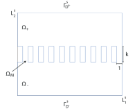
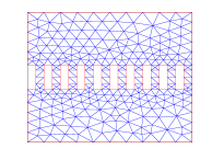
(a)                               (b)

Figure 2: (a) The rescaled computational domain. (b) Adaptive mesh for the computational domain.

The rescaled domain after nondimensionalization is shown in Figure 2-(b). The domain has dimension $L^{s}_{1}\times L^{s}_{2}=2n_{c}\times(2m+1)k$, while the channel has unit base dimension. In the simulation we consider $k=4$. Furthermore, we consider an adaptive triangular mesh as in Figure 2-(b).

The Boundary Conditions

For the electrical potential, we consider the boundary conditions (8), with $\Phi_{1,s}=10^{h}$, $h\in\mathbb{N}$, and $\Phi_{2,s}=0$, that is, for

$$\begin{split}\Phi_{s}(t_{s},x_{s})&=10^{h},\qquad x_{s}\in\Gamma_{D+}^{s};\\ \Phi_{s}(t_{s},x_{s})&=0,\quad\qquad x_{s}\in\Gamma_{D-}^{s};\\ \dfrac{\partial\Phi_{s}}{\partial\nu}(t_{s},x_{s})&=0,\qquad\quad x_{s}\in\partial\Omega^{s}\setminus\Gamma_{D-}^{s}\cup\Gamma_{D-}^{s}.\end{split}$$ (40)

The consequent initial electrical field is shown in Figure 3, in the case $h=4$.

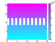
Figure 3: Electrical field with boundary conditions (40).

For the moving ions, in order to simulate ion flow through the system, periodic boundary conditions upon $\partial\Omega$ are applied. In such a way, we may mimic an infinite reservoir and ions are allowed to enter and exit the simulation box.

The Fixed Ions

Two fixed charges have been located in the upper layer of each channel, in order to simulate the behavior of the receptors present in protein channels. As a consequence, the total number of fixed charges is $J=2n_{c}$.

The Ions Dimensions

We consider two different possible dimensions.
The first one refers to a radius of the same scale of the pore, for example $\tilde{\epsilon}\sim 1.52\cdot 10^{-10}$, as in the case of $K+$. In general we consider $\tilde{\epsilon}\sim\epsilon_{1}/4$.
In order to simulate possible cases in which the ion dimension is much smaller than the channel one, we consider also the case $\tilde{\epsilon}\sim\epsilon_{1}/100\sim 10^{-8}$, too.

The Initial Conditions

At the initial time $t=0$ a number of $N$ ions are uniformly distributed in the upper bath $\Omega_{+}$ with normally distributed velocities (see [24]).

Spatial Distribution of Moving Ions

From the definition of the spatial distribution of the moving ions (3), we consider a regularized version via a convolution of the empirical measure (4) by a bivariate normal density $f$ of zero mean and diagonal covariance matrix, and variances $\sigma_{1}^{2},\sigma_{2}^{2},$ that is

$$f*X(x)=\dfrac{1}{N}\displaystyle\sum_{i=1}^{N}f(x_{i}-x),\quad x\in\Omega.$$ (41)

In the following, we consider $\sigma_{1}^{2}=\sigma_{2}^{2}=10^{-1}$.

4.1 Case 1: dimension of the channel $\mathbf{\epsilon_{1}\sim O(10^{-9}m)}$

We simulate the coupled system (22), (35), and (3.4) by taking into account the first scaling factor introduced in Section 3, that is $\epsilon=\epsilon_{1}=10^{-9}$. We consider $N=10^{3}$ free moving ions and boundary conditions (40) with $h=4$. Furthermore, in the membrane we take $n_{c}=10$ channels. The time increment is $dt=10^{-3}$.

Case 1.a. Ion radius $\tilde{\epsilon}\sim\epsilon_{1}/4$

This case is the typical situation of the nanopore. Figure 4 shows the initial distribution of the ions and the state of the system at time $t=3$. It is evident few ions may enter into a channel at the same time.

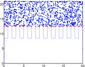
(a) t=0

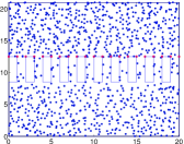
(b) t=3

Figure 4: Initial and final ion locations - Case 1.a.

Figure 5 shows the time evolution of the ion spatial distribution. Since the dynamics are rather fast, after a small time interval at the very beginning of the simulation, the number of ions present in each region is varying but not too much.

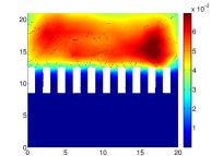
(a) t=0

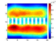
(b) t=1

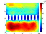
(c) t=2

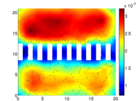
(d) t=3

Figure 5: Time evolution of the ion density - Case 1.a.

This is also visualized in Figure 6, left, showing the time evolution of the number of ions in each region ($\Omega_{+},\Omega_{-}$, and $\Omega_{M}$). Ions are rather dispersed outside the membrane, while inside the ion number is small and not varying too much. On the right-hand side of Figure 6 the distribution of the time spent by a particle into a channel is shown.

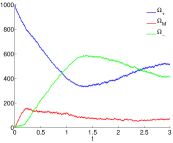
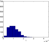
Figure 6: Left: evolution of ion number in $\Omega_{+},\Omega_{-},\Omega_{M}$. Right: histogram of the average time spent by ions in $\Omega_{M}$. Case 1.a.

Case 1.b. Ion radius $\tilde{\epsilon}\sim\epsilon_{1}\cdot 10^{-2}$

Here we consider the simulation results in the same conditions with respect to Case 1.a., but the radius of ions, which is here much smaller. This case corresponds more to the case of micropore.

Figure 7 shows how ions are slower than the previous case. Furthermore, in Figure 8 one may observe that in this case the spatial density of ions in a channel may be significantly greater than zero, a case not observed previously. This is due to fact that here we are reproducing the case in which in each channel one may enter a large number of ions at the same time.

This may be seen in Figure 9, left, where the number of ions in the membrane is clearly higher. As regards to the time needed for crossing a channel, we see how the distribution is less dispersed and is significantly higher in the mean. See also Table 4.

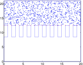
(a) t=0

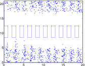
(b) t=3

Figure 7: Initial and final ion locations - Case 1.b.

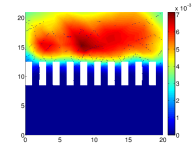
(a) t=0

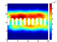
(b) t=1

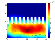
(c) t=2

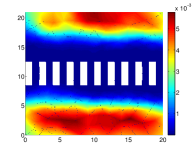
(d) t=3

Figure 8: Time evolution of the ion density - Case 1.b.

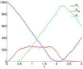
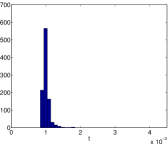
Figure 9: Left: evolution of ion number in $\Omega_{+},\Omega_{-},$ and $\Omega_{M}$. Right: histogram of the average time spent by ions in $\Omega_{M}$. Case 1.b.

4.2 Case 2: dimension of the channel $\mathbf{\epsilon_{1}\sim O(10^{-7}m)}$

Now we simulate the coupled system for the scaling parameter $\epsilon=\epsilon_{1}=10^{-7}$, i.e. with parameters (39).

Case 2.a. Ion radius $\tilde{\epsilon}\sim\epsilon_{1}/4$

Again first we consider the case in which few ions may enter in a channel at the same time, due to the fact that the diameter $\tilde{\epsilon}$ is taken as $\epsilon_{1}/4$

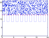
(a) t=0

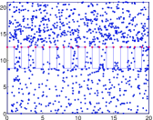
(b) t=3

Figure 10: Initial and final ion locations - Case 2.a.

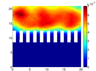
(a) t=0

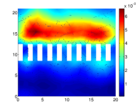
(b) t=1

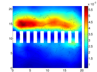
(c) t=2

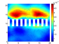
(d) t=3

Figure 11: Time evolution of the ion density - Case 2.a.

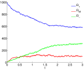
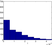
Figure 12: Left: evolution of ion number in $\Omega_{+},\Omega_{-},\Omega_{M}$. Right: histogram of the average time spent by ions in $\Omega_{M}$. Case 2.a.

Due to the fact that the time rescaling (34) is proportional to $\epsilon_{1}$, we expect slower dynamics. This is seen in Figure 12: again the number of ions in the channel region are few, and the velocity of crossing the membrane is smaller. Such dynamics are confirmed by Figure 10–11.

Case 2.b. Ion radius $\tilde{\epsilon}\sim\epsilon_{1}\cdot 10^{-2}$

Now again we consider ions much smaller than the channel. Figure 13 shows the initial distribution of the ions and the state of the system at time $t=3$.

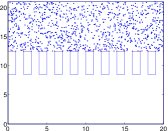
(a) t=0

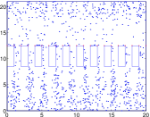
(b) t=3

Figure 13: Initial and final ion locations - Case 2.b.

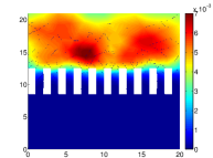
(a) t=0

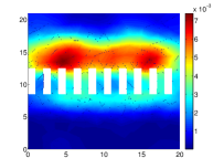
(b) t=1

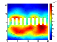
(c) t=2

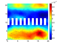
(d) t=3

Figure 14: Time evolution of the ion density - Case 2.b.

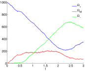
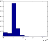
Figure 15: Left: evolution of ion number in $\Omega_{+},\Omega_{-},\Omega_{M}$. Right: histogram of average time spent by ions in $\Omega_{M}$. Case 2.a.

By comparing Figure 7 with Figure 13 and Figure 14 with Figure 8 it is evident that again the density in the channel is higher with respect to the case with bigger ions, but, as already mentioned, speed is higher.

The qualitative behavior of the time evolution of the number of ions in each region in the bath and in the membrane as shown in Figure 15, is similar to the one of case 1.b. in Figure 12.

Quantitative estimates for the four case studies are shown in Tables 3 and 4. The mean time needed by ions for crossing the channel is higher in the case 1.a. and always the mean number of ions in the membrane region are smaller.

Case	Mean	Standard deviation
1.a.	0.0885	0.0400
1.b.	0.1450	0.0142
2.a.	0.1122	0.1065
2.b.	0.1434	0.0503

Table 3: Crossing channel time: mean and standard deviation in the four cases.

Case		$\Omega_{+}$	$\Omega_{-}$	$\Omega_{M}$
1.a.	Mean	498.03	414.59	87.38
	Std	156.97	170.99	30.13
1.b.	Mean	377.71	477.29	144.99
	Std	312.09	334.92	103.75
2.a.	Mean	692.46	206.42	101.11
	Std	109.69	20.93	53.23
2.b.	Mean	518.83	341.35	139.81
	Std	255.30	254.16	96.14

Table 4: Estimates of the number of ions in each region: mean and standard deviation (Std) in the four cases.

4.3 The effective diffusion coefficient

As discussed in [37], the effective diffusion coefficient is different inside and outside the membrane. There are several ways proposed in literature for computing such an estimation [1, 35, 37]. A simple way to estimate the effective diffusion is via the mean square displacement of an ion. In our system, even though the diffusion coefficient governing the randomness of the velocity is constant, the effective diffusion estimated as the mean square displacement of an ion also depends upon on all the exerted nonlinear forces. In particular in the channel, the boundary forces exerted on the ions are much stronger then in the bath, and they also influence the particle mean square displacement.

Split the time interval $[0,T]$ in $L$ time intervals of length $\Delta t$ and let $t^{n}=n\Delta t,n=1,\dots,L$, where we defined for each $\Delta t=10^{-3}$ the Euclidean distance $\delta_{n}^{i}$ as follows:

$$\delta_{n+1}^{i}=||X^{i}(n+1)-X^{i}(n)||_{2}$$

where both $X^{i}(n+1)$ and $X^{i}(n)$, the positions of the $i$th ion at time $t^{n}$ and $t^{n+1}$, lie in a region of the same area $1\times k$ in $\Omega_{M}$, or $\Omega_{+}$; see Figure 2. Let $\delta$ be the sample vector of such distances

$$\delta=(\delta_{1}^{1},\dots,\delta_{1}^{i_{1}},\dots,\delta_{L}^{1},\dots,\delta_{L}^{i_{L}}),$$

where $i_{n}$ is the number of ions feasible for the sample at time $t^{n}$. Let $d=i_{1}+\ldots+i_{L}$ be the size of the sample. We estimated the mean square displacement by unit time by means of the sample variance $V$ of the vector $\delta$ divided by $\Delta t$.

Table 5 shows the estimation of the mean square displacement per unit time in $\Omega_{+}$ and in the membrane $\Omega_{M}$. We may notice how the order of the mean square displacement is smaller in the channel, as expected.

	Region	$V$	$V/\Delta t$	$V_{y}$	$V_{y}/\Delta t$
Case 1a	$\Omega_{M}$	$9.8284\leavevmode\nobreak\ 10^{-4}$	$0.982$	$0.0383$	$38.3020$
	$\Omega_{+}$	$2.9685\leavevmode\nobreak\ 10^{-1}$	$296.8525$	$0.1532$	$153.2315$
Case 1b	$\Omega_{M}$	$5.5878\leavevmode\nobreak\ 10^{-6}$	$0.0056$	$5.4420\leavevmode\nobreak\ 10^{-6}$	$0.0054$
	$\Omega_{+}$	$0.2576$	$257.6380$	$0.2428$	$242.8094$
Case 2a	$\Omega_{M}$	$0.0025$	$2.4511$	$0.0016$	$1.5633$
	$\Omega_{+}$	$0.7206$	$720.6112$	$0.4286$	$428.8674$
Case 2b	$\Omega_{M}$	$0.0054$	$5.3956$	$3.7941\leavevmode\nobreak\ 10^{-4}$	$0.3794$
	$\Omega_{+}$	$0.1381$	$138.0646$	$0.0644$	$64.3650$

Table 5: Estimation of the mean square displacement of ions and per unit time in the $(x,y)$-plane ($V$ and $V/\Delta t$) and along the $y$-direction ($V_{y}$ and $V_{y}/\Delta t$).

5 Discussion

We have considered a fully stochastic mathematical model describing the main characteristics of a multiple channel system, in which ion movement in the bath and throughout membrane channels is modeled in terms of a system of stochastic differential equations, coupled with a Poisson equation, which becomes itself stochastic due to the consequent randomness of the ion positions.

By considering real parameters as in Tables 1 and 2, we have faced the problem of identifying a right scale for the nondimensionalization of the system.

Through a direct comparison of the simulation results of the rescaled system via typical scales of the channels, we see that a first rescaling by a channel size of order $\epsilon_{1}\sim 10^{-10}$ is fast enough to make the dynamics evident. Instead, from Table 3, we may see that the mean time required to cross the membrane is significantly higher in the case of the second rescaling by $\epsilon_{1}\sim 10^{-7}$.

Furthermore, we may notice that with the same rescaling, smaller particles are slower, and a change of velocity is less probable. This is due to the fact that with equal parameters, the smaller the diameter of the ions, the weaker are the forces of Pauling and Lennard–Jones acting on the velocity, since they depend on the ion diameter, as shown by (32) and (31).

The second issue we are interested in is the coupling of the dynamics inside and outside the membrane. This is particularly important in the case of nanopores (cases 1.a. and 2.a). Indeed, as is well shown in Figure 5, while there is a very high number of ions in the bath region, this is not so in the membrane, since the number of ions within each channel becomes very small.

For the time being we propose case 1.a. as a satisfactory rescaling of the system. In such a case, the dynamics have to be maintained to always be stochastic and discrete.

A future step, interesting from the mathematical point of view, is to study the same system when both the number of channels and ions are increasing. The interesting mathematical question, which is relevant also for a reduction of the computational costs in the simulations, concerns the coupling of the two scales regarding the dynamics in the bath and within the channels, with respect to the significant difference in the number of ions per unit volume for the two regions.

As mentioned in the introduction, it is well known that it is reasonable to consider a continuous model for the ion concentrations whenever a law of large numbers may be applied, i.e. when the number of ions per unit volume is sufficiently large. On the other hand such laws cannot be applied in each channel, so that the system has to be kept discrete and stochastic. As a consequence, for a large number of ions in the bath the problem of coupling their dynamics in the bath (averaged continuum ), and inside the channels (discrete and stochastic) arises. An interesting issue refers, in particular, to the transition conditions at the membrane boundaries. As already mentioned, some work in this direction has already been done, for example by Schuss and his collaborators, but, to the best of our knowledge, existing literature has not provided a satisfactory answer yet.

The present study may be regarded as a first step for further investigations that the authors intend to carry on for what it may concern the asymptotic analysis of the Langevin type model for ionic permeation. Moreover, the presented model might be given in a more realistic setting through the introduction of more realistic physiological details, as discussed in the introduction.

Appendix: Computing the rescaled equations

The Poisson Equation. By considering the rescaling (19) and (21), from (6) we rewrite the rescaled term $-\textrm{div}_{x_{s}}{\left(\alpha_{r}\nabla_{x_{s}}\Phi_{s}\left(t_{s},x_{s}\right)\right)}$ involving the rescaled potential field $\Phi_{s}(t_{s},x_{s})$, where $\alpha_{r}$ satisfies (24). Then we have the following:

$$-\textrm{div}_{x_{s}}{\left(\alpha_{r}\nabla_{x_{s}}\Phi_{s}\left(t_{s},x_{s}\right)\right)} = -\epsilon^{2}\textrm{div}_{x}\left(\dfrac{\alpha_{w}}{\alpha_{0}}\nabla_{x}\dfrac{\Phi\left(t,x\right)}{\tilde{\Phi}}\right)$$

$$= -\dfrac{\epsilon^{2}}{\alpha_{0}\tilde{\Phi}}\textrm{div}_{x}\left(\alpha_{w}\nabla_{x}\Phi\left(t,x\right)\right)$$

$$= \dfrac{\epsilon^{2}q}{\alpha_{0}\tilde{\Phi}}\left(z{\displaystyle\frac{1}{N\kappa_{1}}\sum_{k=1}^{N}K_{\kappa_{1}}\left(x-X_{s}^{k}(t)\right)}\right.$$

$$\hskip 28.45274pt\left.+z_{F}{\displaystyle\frac{1}{J\kappa_{2}}\sum_{h=1}^{J}K_{\kappa_{2}}\left(x-X_{s}^{h}(t)\right)}\right)$$

By considering the definition of the interacting kernels (7) and the rescaled ones (23), one obtains

$$-\textrm{div}_{x_{s}}{\left(\alpha_{r}\nabla_{x_{s}}\Phi_{s}\left(t_{s},x_{s}\right)\right)} = -\epsilon^{2}\textrm{div}_{x}\left(\dfrac{\alpha_{w}}{\alpha_{0}}\nabla_{x}\dfrac{\Phi\left(t,x\right)}{\tilde{\Phi}}\right)$$

$$= \dfrac{\epsilon^{2}q}{\alpha_{0}\tilde{\Phi}\epsilon^{3}}\left(z{\displaystyle\frac{1}{N\kappa_{1}^{s}}\sum_{k=1}^{N}U_{1}\left(\epsilon\left(x_{s}-X_{s}^{k}(t_{s})\right)\right)}\right.$$

$$\hskip 36.98866pt\left.+z_{F}{\displaystyle\frac{1}{J\kappa_{2}^{s}}\sum_{h=1}^{J}U_{2}\left(\epsilon\left(x_{s}-Y_{s}^{h}\right)\right)}\right)$$

$$= \dfrac{\epsilon^{2}q}{\alpha_{0}\tilde{\Phi}\epsilon^{3}}\left(z\lambda{\displaystyle\frac{1}{N\kappa_{1}^{s}}\sum_{k=1}^{N}U_{1}^{s}\left(x_{s}-X_{s}^{k}(t_{s})\right)}\right.$$

$$\hskip 36.98866pt\left.+z_{F}\frac{1}{J\kappa_{2}^{s}}\lambda{\displaystyle\sum_{h=1}^{J}U_{2}^{s}\left(x_{s}-Y_{s}^{h}\right)}\right)$$

So, finally, the right-hand side term becomes

$$\dfrac{\epsilon^{2}q}{\alpha_{0}\tilde{\Phi}\epsilon^{3}}\left(z\left(K_{\kappa_{1}^{s}}^{s}*X^{s}(t_{s})\right)(x_{s})+z_{F}\left(K_{\kappa_{2}^{s}}^{s}*Y^{s})\right)(x_{s})\right);$$

hence, by means of the definition (25), we obtain the rescaled Poisson equation (22).

The Langevin system.  The nondimensionalization of the Langevin equations (9)-(2.2) has been done as follows. We scale first the location equation, obtaining, for any $j=1,\dots,N$

$$dX^{j}_{s}\left(t_{s}\right) = \epsilon^{-1}dX^{j}\left(t\right)=\epsilon^{-1}V^{j}\left(t\right)dt$$

$$= \epsilon^{-1}\dfrac{\epsilon}{t_{0}}V^{j}_{s}\left(t_{s}\right)t_{0}dt_{s}=V^{j}_{s}\left(t_{s}\right)dt_{s},$$

that is

$$dX^{j}_{s}\left(t_{s}\right)=V^{j}_{s}\left(t_{s}\right)dt_{s}.$$

Then, we scale the equation describing the evolution of the velocity $V^{j}_{s}$, for any $j=1,\dots,N$. From (20) we have that

$$m_{s}d_{t_{s}}V^{j}_{s}\left(t_{s}\right)=\dfrac{t_{0}}{M\epsilon}md_{t}V^{j}\left(t\right).$$ (42)

Hence, we need to scale the right term in (2.2). Let us denote by $\gamma_{s}$, $\bar{\sigma}$, and $M_{S}$, the nondimensionalized friction, diffusion coefficient, and mass, respectively, such that

$$\gamma=\bar{\gamma}\gamma_{s};\quad\sigma=\sigma_{s}\bar{\sigma}\quad m=Mm_{s}.$$

From the Stokes-Einstein relation and (12) we have

$$m_{s}\gamma_{s}=\dfrac{K_{B}T}{DM\bar{\gamma}},\quad\sigma=\sqrt{2K_{B}TMm_{s}\bar{\gamma}\gamma_{s}};$$

hence, $\bar{\sigma}=\sqrt{2K_{B}TM\bar{\gamma}}$. From the definition of the rescaled potential (21), the electrical field becomes

$$\nabla_{x}\phi\left(t,x\right)=\dfrac{K_{B}T}{q}\frac{1}{\epsilon}\nabla_{x_{s}}\phi_{s}\left(t_{s},x_{s}\right).$$

The forms of the interacting term are the same as in the dimensionalized term. Indeed, the Pauling potential (13) becomes

$$H_{P}\left({r}\right)=\dfrac{\left(\epsilon(r_{1,s}+r_{2,s})\right)^{10}}{\left(\epsilon r_{s}\right)^{9}}=\dfrac{\epsilon\left(r_{1,s}+r_{2,s}\right)^{10}}{\left(r_{s}\right)^{9}}$$

and

$$\nabla_{x}{H^{*}_{P}\left[\nu_{X}(t)+\nu_{Y}\right](x)} = \nabla_{x_{s}}\left(\sum_{k=1}^{N}\dfrac{\left(r_{1,s}+r_{2,s}\right)^{10}}{|x_{s}-X_{s}^{k}(t_{s})|^{9}}+\sum_{h=1}^{J}\dfrac{\left(r_{1,s}+r_{2,s}\right)^{10}}{|x_{s}-Y_{s}^{h}|^{9}}\right)$$

$$= \nabla_{x_{s}}H^{s,*}_{P}\left[\nu^{s}_{X}(t)+\nu^{s}_{Y}\right](x),$$

where, given a distance $r_{s}$ in the new coordinate scale, we have defined the scaled Pauling potential as follows:

$$H^{s}_{P}\left(r_{s}\right)=\dfrac{\left(r_{1,s}+r_{2,s}\right)^{10}}{r_{s}^{9}}.$$

In a same way it is possible to scale the Lennard–Jones potential (17). For the distance from the border $d_{\partial{\Omega}}$ defined in (15) we have that

$$\begin{split}d_{\partial{\Omega}}\left(\epsilon x_{s}\right)&=\min_{\epsilon\leavevmode\nobreak\ y_{s}\in{\partial{\Omega}}}{|\epsilon\leavevmode\nobreak\ x_{s}-\epsilon\leavevmode\nobreak\ y_{s}|}\\ &=\epsilon\leavevmode\nobreak\ \min_{y_{s}\in{\partial{\Omega_{s}}}}{|x_{s}-y_{s}|}\\ &=\epsilon\leavevmode\nobreak\ d_{\Omega_{s}}^{s}\left(x_{s}\right),\end{split}$$

where $d_{\Omega_{s}}^{s}\left(x_{s}\right)$ is the distance of the point $x_{s}$ from the membrane boundary in the new scale. The potential $\widetilde{H}_{LJ}$ is scaled as follows:

$$\begin{split}\widetilde{H}_{LJ}\left(\epsilon r_{s}\right)&=\epsilon\varepsilon_{LJ}^{s}\left[\left(\dfrac{2R_{vdW}}{\epsilon r_{s}}\right)^{12}-2\left(\dfrac{2R_{vdW}}{\epsilon r_{s}}\right)^{6}\right]\\ &=\epsilon\varepsilon_{LJ}^{s}\left[\left(\dfrac{2R^{s}_{vdW}}{r_{s}}\right)^{12}-2\left(\dfrac{2R^{s}_{vdW}}{r_{s}}\right)^{6}\right]\end{split}$$

where $\varepsilon_{LJ}^{s}$ is the nondimensionalization of the size of $\varepsilon_{LJ}$ which depends on length, and $R_{vdW}^{s}$ is the scaled van der Waals radii. If we define the rescaled truncated shifted Lennard–Jones potential as

$$\widetilde{H}_{LJ}^{s}\left(x_{s}\right)=\varepsilon_{LJ}^{s}\left[\left(\dfrac{2R^{s}_{vdW}}{x_{s}}\right)^{12}-2\left(\dfrac{2R^{s}_{vdW}}{x_{s}}\right)^{6}\right],$$

it follows that

$$\widetilde{H}_{LJ}\left(x\right)=\epsilon\widetilde{H}_{LJ}^{s}\left(x_{s}\right).$$

For the random term, we rescaled the Wiener process $W^{j}_{t}$ and obtained $W^{j}_{t}=W^{j}_{t_{0}t_{s}}\sim\sqrt{t_{0}}W^{j}_{t_{s}}$, where $W^{j}_{t_{s}}$ is a Wiener process with respect to time $t_{s}$.

Finally, by gathering together all the previous terms, from (42) and (2.2) we have the following:

$$m_{s}d_{t_{s}}V^{j}_{s}\left(t_{t_{s}}\right) = -\dfrac{t_{0}^{2}}{M\epsilon}\left[Mm_{s}\bar{\gamma}\gamma_{s}\dfrac{\epsilon}{t_{0}}V^{j}_{s}(t_{s})+z\leavevmode\nobreak\ q\dfrac{K_{B}T}{\epsilon q}\nabla_{x_{s}}\Phi_{s}\left(t_{s},X^{j}_{s}\right)\right.$$

$$\hskip 34.14322pt+F_{I}\nabla_{x_{s}}H_{P}^{s,*}\left[\nu_{X}^{s}(t_{s})+\nu_{Y}^{s}\right](X^{j}(t_{s}))$$

$$\hskip 34.14322pt+F_{I}\nabla_{x_{s}}H_{LJ}^{s}\left(d_{\partial{\Omega_{s}}}^{s}(X^{j}(t_{s}))\right)\bigg{]}dt_{s}$$

$$+\dfrac{t_{0}\sqrt{t_{0}}}{M\epsilon}\sqrt{2K_{B}TM\bar{\gamma}m_{s}\gamma_{s}}dW^{j}_{t_{s}}.$$

By considering the relation (30) between $\sigma_{s}$ and $\gamma_{s}$,

$$m_{s}d_{t_{s}}V^{j}_{s}\left(t_{t_{s}}\right) = -\left[{\bar{\gamma}}{t_{0}}m_{s}\gamma_{s}V^{j}_{s}\left(t_{s}\right)-\dfrac{t_{0}K_{B}T}{M\epsilon^{2}}\nabla_{x_{s}}\Phi_{s}\left(t_{s},X^{j}_{s}\right)\right.$$

$$\hskip 14.22636pt+\dfrac{F_{I}t_{0}^{2}}{M\epsilon}\left(\nabla_{x_{s}}{H_{P}^{s,*}}\left[\nu_{X}^{s}(t_{s})+\nu_{Y}^{s}(X^{j}_{s}(t_{s}))\right]+\nabla_{x_{s}}{H_{LJ}^{s}}\left(d_{\partial{\Omega_{s}}}\right)\right)\bigg{]}dt_{s}$$

$$+\dfrac{t_{0}\sqrt{t_{0}}}{M\epsilon}\sqrt{K_{B}TM\bar{\gamma}}\sigma_{s}dW^{j}_{t_{s}}.$$

Thus, we have obtained the Langevin system (28), (3.3), and (33).

References

- [1] T. W. Allen, S. Kuyucak, S. H. Chung, Molecular dynamics estimates of ion diffusion in model hydrophobic and KcsA potassium channels, Biophysical Chemistry 86(1): 1–14, 2000.
- [2] M. Burger, M. B. Schlake, M. T. Wolfram, Nonlinear Poisson equations for ion flux through confined geometries, Nonlinearity, 25(2): 961, 2012.
- [3] V. Capasso, D. Morale, Asymptotic Behavior of a System of Stochastic Particles subject To Nonlocal Interactions, Stochastic Analysis and Applications, 27, 3, 574 – 603, 2009.
- [4] V. Capasso, D. Morale, G. Facchetti, The role of stochasticity in a model of retinal angiogenesis, IMA Journal of Applied Mathematics, 77, 729-747, 2012.
- [5] V. Capasso, D. Morale, G. Facchetti, Randomness in self-organized phenomena. A case study: Retinal angiogenesis, BioSystems, 112, 292 -297, 2013.
- [6] X. Chen, R. Ji, M. Steinhart, A. Milenin, K. Nielsh, U. Gsele, Aligned horizontal silica nano channels by oxidative self-sealing of patterned silicon wafers, Chem. Mater. 19,3–5, 2007.
- [7] B. Corry, S. Kuyucak, S. H. Chung, Tests of continuum theories as models of ion channels. II. Poisson–Nernst–Planck theory versus Brownian dynamics, Biophysical Journal, 78(5): 2364–2381, 2000.
- [8] B. Corry, S. Kuyucak, S. H. Chung, Test of Poisson theory in ion channels, Letter to the editor, J. Gen. Physiol 114(1–2), 597–599, 1999.
- [9] B. Corry, T. W. Allen, S. Kuyucak, S. H. Chung, Mechanisms of permeation and selectivity in calcium channels, Biophysical Journal, 80(1): 195–214, 2001.
- [10] C. E. Dangerfield, D. Kay , K. Burrage, Modeling ion channel dynamics through reflected stochastic differential equations, Physical Review E 85 (5), 051907, 2012.
- [11] D. A. Doyle, J. Morais Cabral, R. A. Pfuetzner, A. Kuo, J. M. Gulbis, S. L. Cohen, B. T. Chait, R. MacKinnon, The structure of the potassium channel: molecular basis of K+ conduction and selectivity. Science 280: 69–77, 2008.
- [12] R. S. Eisenberg, M. M. Klosek, Z. Schuss, Diffusion as a chemical reaction: Stochastic trajectories between fixed concentrations, J. Chem. Phys., 102, 1767-1780, 1995.
- [13] B. Eisenberg, Y. Hyon, C. Liu, Energy Variational Analysis EnVarA of Ions in Water and Channels: Field Theory for Primitive Models of Complex Ionic Fluids, Journal of Chemical Physics 133, 104104, 2010
- [14] B. Eisenberg , Mass Action in Ionic Solutions, Chemical Physics Letters, , 511, 1-6, 2011.
- [15] B. Eisenberg , Crowded charges in ion channels, Advances in Chemical Physics, 148 (eds S. A. Rice and A.R. Dinner), 2011.
- [16] B. Eisenberg , Ions in Fluctuating Channels: Transistors Alive, Fluctuation and Noise Letters , 11, 76-96, 2012.
- [17] B. Eisenberg , Ion Interactions are everywhere, Physiology , 28, 28-38, 2013.
- [18] R. Erban From molecular dynamics to Brownian dynamics. Proc. R. Soc. A 470: 20140036, 2014
- [19] T. C. Lin, B. Eisenberg, A new approach to the Lennard-Jones potential and a new model: PNP-steric equations, Communications in Mathematical Sciences, 12(1), 149 173, 2014.
- [20] J. L. Liu, B. Eisenberg, Poisson-Nernst-Planck-Fermi theory for modeling biological ion channels, The Journal of Chemical Physiscs, 141, 22D532, 2014.
- [21] B. Hille, Ionic Channels of Excitable Membranes, Sinauer Associates Inc., 3rd Edition, 2001.
- [22] W. Im, S. Seefeld, B. Roux, A grand canonical Monte Carlo–Brownian dynamics algorithm for simulating ion channels, Biophysical Journal, 79(2): 788–801, 2000.
- [23] W. Im, S. Seefeld, B. Roux Brownian dynamics simulations of ions channels: a general treatment of electrostatic reaction fields for molecular pores of arbitrary geometry, Journal of Chemical Physics, 115(10): 4850–4861, 2001.
- [24] D. Marreiro, M. Saraniti, S. Aboud, Brownian dynamics simulation of charge transport in ion channels, Journal of Physics: Condensed Matter, 19(21): 215203, 2007.
- [25] P. A. Markowich, C. A. Ringhofer, C. Schmeiser, Semiconductor Equations, Springer–Verlag, 1990.
- [26] E. Moro, Hybrid method for simulating front propagation in reaction-diffusion systems, Physycal Review E, 69, 060101(R), 2004.
- [27] G. Moy, B. Corry, S. Kuyucak, S. H. Chung, Tests of continuum theories as models of ion channels. I. Poisson–Boltzmann theory versus brownian dynamics, Biophysical Journal, 78(5): 2349–2363, 2000.
- [28] G. Moy, B. Corry, S. Kuyucak, S. H. Chung, Invalidity of continuum theories of electrolytes in nanopores, Chem. Phys. Lett. 320(1): 35–41, 2000.
- [29] B. Nadler, Z. Schuss, A. Singer, R. S. Eisenberg, Diffusion through protein channels: From molecular description to continuum equations, Nanotechnology, 3: 439–442, 2003.
- [30] N. Nadler, Z. Schuss, A. Singer, R. S. Eisenberg, Ionic diffusion through confined geometries: from Langevin equations to partial differential equations, Journal of Physics: Condensed Matter, 16(22): S2153, 2004.
- [31] B. Nadler, Z. Schuss, A. Singer., Langevin trajectories between fixed concentrations, Phys. Rev. Lett., 94(21): 218101, 2005.
- [32] S. V. Nedea, A. J. H. Frijns, A. A. van Steenhoven, A. J. Markvoort, P. A. J. Hilbers, Hybrid method coupling molecular dynamics and Monte Carlo simulations to study the properties of gases in microchannels and nanochannels, Physical Review E, 72(1): 016705, 2005.
- [33] B. A. Yi and L. Y. Jan, Ion channels in Encyclopedia of the Human Brain, Academic Press, 2002.
- [34] M. A. Peletier, M. Röger, Partial Localization, Lipid Bilayers, and the Elastica Functional, Arch. Rational Mech. Anal., 193, 475 -537, 2009.
- [35] Y. Pokern, A. M. Stuart,, E. Vanden-Eijnden, Remarks on Drift Estimation for Diffusion Processes, Multiscale Model. Simul., 8(1), 69 -95, 2009.
- [36] P. Ramirez, M. Aguilella–Arzo, A. Alcaraz, J. Cervera, V. M. Aguilella, Theoretical description of the ion transport across nanopores with titratable fixed charges: Analogies between ion channels and synthetic pores, Cell biochemistry and biophysics, 44(2): 287–312, 2006.
- [37] G. R. Smith, M. S. P. Sansom, Dynamic Properties of Na1 Ions in Models of Ion Channels: A Molecular Dynamics Study, Biophysical Journal, 75, 1998
- [38] C. Schmeiser, A model for the transient behavior of long-channel MOSFETs, SIAM Journal on Applied Mathematics, 54(1): 175–194, 1994.
- [39] M. Schmuck, New porous medium Poisson-Nernst-Planck equations for strongly oscillating electric potentials, Journal of Mathematical Physics,54, 021504, 2013.
- [40] M. Schmuck , M.Z. Bazant, Homogenization of the Poisson-Nernst-Planck equations for transport in charged porous media, arXiv:1202.1916v2, 2014.
- [41] Z. Schuss, B. Nadler, R. S. Eisenberg, Derivation of Poisson and Nernst-Planck equations in a bath and channel from a molecular model, Physical Review E, 64, 036116, 2001.
- [42] I. Vlassiouk, S. Smirnov, and Z. Siwy, Ionic selectivity of single nano channels, Nano Letters 8(7): 1978–1985, 2008.
- [43] R. J. Williams, W. A. Zheng, On reflecting brownian motion – a weak convergence approach., Ann. Inst. Henri Poincaré, , 26(3), 461–488,1990.
- [44] Zheng, J. , M. C. Trudeau, Handbook of ion channels, CRC Press, 2015.