How stochastic synchrony could work in cerebellar Purkinje cells

Abstract

Simple spike synchrony between Purkinje cells projecting to a common neuron in the deep cerebellar nucleus is emerging as an important factor in the encoding of output information from cerebellar cortex. Stochastic synchronization is a viable mechanism through which this synchrony could be generated, but it has received scarce attention, perhaps because the presence of feedforward inhibition in the input to Purkinje cells makes insights difficult. This paper presents a method to account for feedforward inhibition so the usual mathematical approaches to stochastic synchronization can be applied. Three concepts (input correlation, heterogeneity, and PRC shape) are then introduced to facilitate an intuitive understanding of how different factors can affect synchronization in Purkinje cells. This is followed by a discussion of how stochastic synchrony could play a role in the cerebellar response under different assumptions.

1 Introduction

The cerebellum has a striking and relatively clear anatomical organization, which has brought hope that it could be the first brain system whose function could be understood in terms of its structure [1]. There is agreement that the cerebellum may play a role in a variety of cognitive functions, in addition to its involvement in motor control [2].

Figure 1 shows the basic anatomical organization of the cerebellar cortex. See [3] or [1] for reviews. In order to designate specific types of neurons and axons in the cerebellum the abbreviations of figure 1 will be used. Synapses from a source neuron/axon type towards a target neuron type will be denoted by the abbreviation of the source and target connected by a dash; e.g. PF-PC denotes the synapse between parallel fibers and Purkinje cells.

Figure 1: Basic connection scheme of the cerebellum. Granule cells (GC) receive afferent and efferent information from the mossy fibers (MF), and convey that information through their parallel fibers (PF). The PFs excite both Purkinje Cells (PC) and molecular layer interneurons (MLI); in turn the MLIs send axons to the PCs. Purkinje cells constitute the only output of the cerebellar cortex, and they send axons that form GABAergic inhibitory connections on the cells of the deep cerebellar nuclei (DCN). Neurons in the inferior olivary nucleus (IO) send axons known as climbing fibers (CF) which form thousands of synapses on PCs. Each PC receives excitation from a single CF. An action potential in a CF reliably causes an action potential in the PCs it innervates; these action potentials are known as complex spikes, and are easily distinguishable from simple spikes, which are action potentials tonically generated by the PC, and modulated by the PFs. Not illustrated in the figure is the fact that the ascending axons (AA) of the granule cells can make multiple connections on the dendritic arbor of PCs [4], the orientation of PC dendritic arbors perpendicular to parallel fibers, or the organization in parasagittal modules [5].

Perhaps the most influential set of ideas regarding how the cerebellum works is the Marr/Albus model [6, 7], which has led to a variety of models in which Purkinje cells act like a perceptron whose learning signal comes from the climbing fibers. (e.g. [8, 9, 10, 11, 12, 13, 14]). The discovery of conjunctive Long-Term Depression (LTD) in the PF-PC synapses [15, 16, 17] has added plausibility to these models. Over time, however, it has become increasingly clear that conjunctive LTD alone may not explain learning in the cerebellum.

Several studies suggest the incompleteness of conjunctive LTD to explain cerebellar learning. First, it has been shown that cerebellar motor learning can take place in the absence of PF-PC LTD [18, 19]. Second, the correlation of Purkinje cell firing and muscle EMG can show both positive or negative correlations, with positive correlations being the more prevalent [20, 21]. If the role of Purkinje cells was to gate motor commands through just inhibition, negative correlations should be the most common. Third, synaptic inhibition of Purkinje cells, whose complex spike-elicited plasticity acts to counteract PF-PC conjunctive LTD, seems to play a role in motor learning [22], which is ignored by models that rely exclusively on PF-PC LTD. Moreover, other studies suggest that the timing of Purkinje cells’ spikes is important, not only their firing rate. Tottering mutant (tg) mice have virtually the same firing rate as that of wild types during spontaneous activity and in response to optokinetic stimulation; nevertheless, tg mutants show abnormal compensatory eye movements and severe ataxia [23].

When explaining how the timing of PC simple spikes affect their DCN targets, and how different types of CF-mediated plasticity affect cerebellar output, it may be important to pay attention to synchrony among Purkinje cells innervating the same DCN cell. This syncrony can modulate the response of the target DCN cell [24, 25, 26, 27]. It has been observed that there exists simple-spike synchrony among PCs separated by several hundred micrometers, and that this synchrony seems to depend on afferent input [28, 29, 30, 31, 32]. This synchrony does not seem to be fully explained by firing rate co-modulation or PC recurrent collaterals. Firing rate modulation may be insufficient in this case, because there are cases where the modulation in synchrony is unrelated to the modulation in firing rate [29, 30]. Purkinje cell recurrent collaterals tend to generate oscillations whose coherence decays with distance [33], which is inconsistent with the distances across which synchrony is found; moreover, it is unclear how sensory inputs could modify the functional coupling of Purkinje cells [31] if this coupling depended on a fast oscillatory regime. It is thus appropriate to study stochastic synchronization as a candidate mechanism to explain how Purkinje cells can activate synchronously.

The phenomenon of stochastic synchrony happens when several uncoupled oscillators synchronize their phases when receiving correlated inputs [34, 35]. The intuition behind this is that if the oscillators become entrained to the inputs then they will respond similarly, thus acquiring similar phases. An interesting aspect of stochastic synchronization is that the degree of synchrony can be controlled by the way that the oscillators respond to inputs, which opens the possibility of its modulation by plasticity mechanisms. If synchrony plays a role in shaping the response of cerebellar cortex, it seems feasible that there are plasticity mechanisms capable of creating synchrony.

One possible reason why stochastic synchrony has not been largely considered in the case of Purkinje cells is the complication arising from the feedforward inhibition in the parallel fibers. As shown in figure 1, PFs stimulate MLIs, which in turn stimulate PCs. This inhibition has been observed as IPSPs arising shortly after EPSPs [36], and seems to be fundamental in understanding the response of PCs [37, 38]. Although considerable advances have been made in understanding stochastic synchrony [34, 35, 39, 40, 41, 42, 43, 44, 45, 46, 47, 48, 49, 50], no study has explored how feedforward inhibition affects this process.

Exploring stochastic synchronization of Purkinje cells requires to represent their activity in terms of their phase. A neuron that fires periodically can be understood as a dynamical system whose trajectory in phase space follows an asymptotically stable limit cycle. Such a dynamical system can be described by a single variable called its phase; the phase describes how far the current state is along the limit cycle trajectory. Perturbations to the system (such as synaptic inputs in the case of a neuron) can be described by how they shift the phase of the system when they are received [51, 52]. The PRC (Phase Response Curve or Phase Resetting Curve) of the system plots the shift in phase that an input produces as function of the system’s phase when the input is received. PRCs are a standard tool when understanding the behavior of coupled oscillators, and have been extensively used to describe networks of neurons [53, 54]. Also, as expected, PRCs are also a standard tool in analytical studies of stochastic synchronization.

This paper presents two main sets of results. The first one is the development of an equivalent PRC. If the effect of feedforward excitation coming from the PFs to the PCs is represented with an excitatory PRC, and the effect of feedforward inhibition coming to the PCs from the MLIs is represented with an inhibitory PRC, the equivalent PRC lumps the effect of both excitatory and delayed inhibitory PRCs so we only have one type of inputs. This allows the insights from the theory of stochastic synchronization to be applied when there is feedforward inhibition, as is the case of Purkinje cells. The equivalent PRC is defined in two different ways, and in order to validate these definitions Monte Carlo simulations are performed to verify that an oscillator using the equivalent PRC responds similarly to an oscillator with excitatory and delayed inhibitory inputs.

The second set of results in this paper consists of computational simulations of oscillators receiving correlated noise and feedforward excitation and delayed feedforward inhibition. These simulations show that, as expected, the results from the theory of stochastic synchronization can provide valuable insights about the factors which cause synchrony. In order to explore how stochastic synchrony may affect cerebellar output, I focus on 3 factors (input correlation, heterogeneity, and PRC shape) that control the level of synchronization, and on how they may be affected by CF-mediated plasticity. The output of the synchronizing oscillators is in turn directed towards an oscillator representing a DCN cell, which includes a simple mechanism to produce rebound spikes (spikes caused from powerful depolarizing currents activated by membrane hyperpolarization; they can raise the firing rate in response to an increase in synchrony). Through the use of this model it is shown that synchronization is a subtle response that can depend on several physiological details not often considered in the literature. For example, for the parameters used: (1) synchrony among Purkinje cells does not have to be related to their firing rate modulation, and (2) the effect of synchrony could complement or oppose the putative effect of LTD in the PF-PC synapse. The paper ends with a discussion of how some hypotheses regarding cerebellar function may change when synchrony is taken into account.

2 Models

The equivalent PRC mentioned above will be developed in the next three subsections. This equivalent PRC can only emulate the effects of excitation and delayed inhibition in an approximate manner, and there are several ways to define it. This paper presents two different definitions for the equivalent PRC. The first subsection of this section presents introductory material, and the next two subsections develop the two different definitions of the equivalent PRC.

2.1 Reduction to a phase equation, and the stationary phase PDF

This subsection briefly outlines some basic results from [52, 51] using notation based on [39]. The results show how $N$ dynamical systems oscillating in a limit cycle and receiving impulsive inputs can be represented with $N$ phase variables. PRCs, the phase transition function, and the phase evolution equation are introduced for individual oscillators, which allows to find an equation for their stationary phase Probability Density Function (PDF). If we measure the phase of the oscillator at some random point in time, the phase PDF can provide the probability that the sampled phase is in a particular interval.

Consider $N$ oscillators whose dynamics can be expressed as

$$\mathbb{\dot{X}}_{i}(t)=\mathbb{F}(\mathbb{X}_{i}(t))+\mathbb{I}_{i}(t)$$ (1)

for $i=1,\dots,N$, where the vector $\mathbb{X}_{i}(t)$ denotes the state of oscillator $i$ at time $t$, $\mathbb{F}$ is the function describing the dynamics of each oscillator, and $\mathbb{I}_{i}(t)$ represents external random inputs consisting of impulsive displacements in phase space. We assume that the oscillators have an asymptotically stable limit cycle $\mathbb{X}_{0}(t)$. The impulsive inputs are given by

$$\mathbb{I}_{i}(t)=\sum_{n=1}^{\infty}\mathbb{e}_{n}^{i}\delta(t-t_{n}^{i})$$ (2)

where $t_{n}^{i}$ represents the time of the $n$-th input to the $i$-th oscillator, and $\mathbb{e}_{n}^{i}$ provides the direction of the shift in phase space caused by the corresponding input, so that at time $t_{n}^{i}$ the oscillator $i$ receives an immediate shift in phase space from point $\mathbb{X}_{i}$ to point $\mathbb{X}_{i}+\mathbb{e}_{n}^{i}$. Since our oscillator represents a neuron, the value of $\mathbb{e}_{n}^{i}$ should be determined by the synapse that receives the input. Furthermore, it is assumed that the inputs will not take the system outside the basin of attraction of $\mathbb{X}_{0}(t)$. The inputs that will be considered in this paper behave as Poisson random point processes. If an input has a mean firing rate $r$, then its interimpulse interval $T$ has an exponential distribution:

$$P(T)=r\text{e}^{-rT}$$ (3)

where $P(T)$ is the probability density function for $T$.

We define a phase variable $\theta$ along the limit cycle so that $\theta(t)=\theta(\mathbb{X}_{0}(t))$, $\theta$ has a constant angular velocity $\omega$, and its range is $[0,1)$. This means that in the absence of external inputs we’ll have:

$$\dot{\theta}_{i}(t)=\omega_{i}.$$ (4)

In the first part of the results section we work with systems where all the oscillators have the same angular frequency $\omega$. The phase of points not directly on $\mathbb{X}_{0}$ is defined through the use of isochrons, which are the set of points that asymptotically converge to a particular trajectory $\mathbb{X}^{*}_{0}$ in the periodic orbit. If the points on an isochron converge to the trajectory $\mathbb{X}^{*}_{0}$, then their phase at time $t$ is $\theta(\mathbb{X}^{*}_{0}(t))$. For all functions in this paper whose arguments include a phase value, I assume that this phase value is taken modulo 1; e.g. phases $0$, $1$ are the same phase, and the same can be said of phases $-0.1$, $0.9$, and $2.9$. When an oscillator has phase $\theta$ at time $t$, and an input shifts its state at that moment by an amount $\mathbb{e}$ then this state moves to a new isochron, with the consequent shift in phase denoted by $G(\theta,\mathbb{e})$. We define the phase transition function as

$$F(\theta,\mathbb{e})=\theta+G(\theta,\mathbb{e}),$$ (5)

with its output taken modulo 1. If the phase of an oscillator at time $t_{n}$ right before its $n$-th input is $\theta_{n}$, then the phase right after the input can be written as $\phi_{n}\equiv F(\theta_{n},\mathbb{e}_{n})=\theta_{n}+G(\theta_{n},\mathbb{e}_{n})$. The evolution equation of the phase is an iterative equation describing the phase of the oscillator at the time when the $(n+1)$-th input arrives:

$$\theta_{n+1}=\omega T_{n}+F(\theta_{n},\mathbb{e}_{n})=\theta_{n}+\omega T_{n}+G(\theta_{n},\mathbb{e}_{n}),$$ (6)

where $T_{n}=t_{n+1}-t_{n}$. The dynamics of the phase in continuous time are described by the equation:

$$\dot{\theta}(t)=\omega+\sum_{n=1}^{\infty}G(\theta_{n},\mathbb{e}_{n})\delta(t-t_{n}).$$ (7)

Given that the input times $t_{n}$ and the input effects $\mathbb{e}_{n}$ are random variables, so are the phases $\theta_{n}$. The Probability Density Function (PDF) of the phase $\theta$ at time step $n$ is denoted $\rho(\theta,n)$. This PDF can be described by the following generalized Frobenius-Perron equation [55]:

$$\rho(\theta,n+1)=\int_{0}^{1}W(\theta-\phi)\int Q(\mathbb{e})\int_{0}^{1}\delta(\phi-F(\psi,\mathbb{e}))\rho(\psi,n)\ d\psi\ d\mathbb{e}\ d\phi.$$ (8)

The term $W(\theta-\phi)$ represents the probability that during the interimpulse interval $T_{n}$ the phase changes from $\phi$ to $\theta$. $Q(\mathbb{e})$ is the probability density function for $\mathbb{e}$. Intuitively, the two innermost integrals produce the expected phase after the $n$-th input with $\psi$ being the starting phase; this expected phase, represented by the integration variable $\phi$ is taken in the outermost integral in order to calculate the probability that during the interspike interval the phase transitions from $\phi$ to $\theta$. The transition kernel $W(\theta)$ can be explicitly obtained in the case of Poisson inputs, considering that its arguments are taken to be modulo 1:

$$W(\theta) =\frac{1}{\omega}\sum_{j=0}^{\infty}P\left(\frac{\theta+j}{\omega}\right)=\frac{r}{\omega}\sum_{j=0}^{\infty}\text{e}^{-\frac{r}{\omega}\theta}\text{e}^{-\frac{r}{\omega}j}$$

$$=\frac{A\text{e}^{-A\theta}}{1-\text{e}^{-A}},$$ (9)

with $A=r/\omega$. In the limit of a large number of transitions the PDFs $\rho(\theta,n)$ will reach a stationary state $\rho(\theta)$ obeying:

$$\rho(\theta)=\int_{0}^{1}W(\theta-\phi)\int Q(\mathbb{e})\int_{0}^{1}\delta(\phi-F(\psi,\mathbb{e}))\rho(\psi)\ d\psi\ d\mathbb{e}\ d\phi.$$ (10)

I refer to this equation as the phase PDF equation.

2.2 The equivalent PRC as a function of the phase PDF

The first idea to obtain an equivalent PRC, denoted in this subsection as $\Delta$, is to take the phase PDF $\rho(\theta)$ produced by the excitatory and inhibitory inputs, and define $\Delta$ so its phase PDF matches $\rho(\theta)$. This idea will be developed below.

I start by assuming a single oscillator and a single Poisson process that produces excitatory inputs. Feedforward inhibition is modeled by assuming that for each excitatory input at time $t_{n}$ there will be a corresponding inhibitory input at time $t_{n}+d$, where $d$ represents the feedforward delay. All excitatory inputs will produce a shift in phase space $\mathbb{e}_{exc}$, whereas inhibitory inputs produce a shift $\mathbb{e}_{inh}$. The excitatory and inhibitory PRCs are defined respectively as: $\Delta_{exc}(\theta)=G(\theta,\mathbb{e}_{exc})$, $\Delta_{inh}(\theta)=G(\theta,\mathbb{e}_{inh})$, where the function $G$ maps shifts in phase space to shifts in phase. An oscillator using instead the equivalent PRC will present a shift in phase $\Delta(\theta)$ at the times when the excitatory inputs arrive.

I assume a perturbation from the system where the PRC is zero for all phases and the phase PDF is uniform. Furthermore, the perturbation is small enough so that the phase transition function $F$ is still invertible. Let $\rho(\theta)=1+\varepsilon\rho_{1}(\theta)$, and expand the equivalent PRC as $\Delta(\theta)=\varepsilon\Delta_{1}(\theta)+\varepsilon^{2}\Delta_{2}(\theta)+O(\varepsilon^{3})$ (using big Oh notation), so that as $\varepsilon$ goes to zero we recover the unperturbed system. Before substituting these terms, the phase PDF equation 10 is simplified in 3 steps:

1. The middle integral disappears, since there is only one type of input, and the PDF $Q$ integrates to one.

2. We perform the innermost integral using the basic formula for performing change of variables with Dirac $\delta$ functions. If $g(x)$ is a real function with a root at $x_{0}$ the formula is $\delta(g(x))=\frac{\delta(x-x_{0})}{|g^{\prime}(x_{0})|}$.

3. We substitute the transition kernel $W$ for its expression in Eq. 9.

This yields:

$$\rho(\theta)=\int_{0}^{1}\frac{A\text{e}^{-A(\theta-\phi)}}{1-\text{e}^{-A}}\frac{\rho(F^{-1}(\phi))}{|F^{\prime}(F^{-1}(\phi))|}\ d\phi$$ (11)

Notice that the argument $(\theta-\phi)$ of $W$ is still taken modulo 1, so we need separate integrals for the cases when this argument is positive and negative:

$$\rho(\theta)=\frac{A\text{e}^{-A\theta}}{1-\text{e}^{-A}}\left[\int_{0}^{\theta}\text{e}^{A\phi}\frac{\rho(F^{-1}(\phi))}{|F^{\prime}(F^{-1}(\phi))|}\ d\phi+\text{e}^{-A}\int_{\theta}^{1}\text{e}^{A\phi}\frac{\rho(F^{-1}(\phi))}{|F^{\prime}(F^{-1}(\phi))|}\ d\phi\right].$$ (12)

We now assume $F(\phi)=\phi+\varepsilon\Delta_{1}(\phi)+\varepsilon^{2}\Delta_{2}(\phi)+O(\varepsilon^{3})$. Let $F^{-1}(\phi)=\phi+\varepsilon\psi_{1}(\phi)+\varepsilon^{2}\psi_{2}(\phi)+O(\varepsilon^{3})$. Substituting these two previous expressions in the identity $F(F^{-1}(\phi))=\phi$ we obtain:

$$\psi_{1} =-\Delta_{1},$$

$$\psi_{2} =-\Delta_{2}+\Delta_{1}\Delta_{1}^{\prime},$$

$$F^{-1}(\phi) =\phi-\varepsilon\Delta_{1}+\varepsilon^{2}(\Delta_{1}\Delta_{1}^{\prime}-\Delta_{2})+O(\varepsilon^{3}),$$

where the argument has been omitted in some functions for brevity of notation. Using this expression for $F^{-1}$ we find:

$$\frac{\rho(F^{-1}(\phi))}{|F^{\prime}(F^{-1}(\phi))|}=\frac{1+\varepsilon\rho_{1}-\varepsilon^{2}\Delta_{1}\rho_{1}^{\prime}+O(\varepsilon^{3})}{1+\varepsilon\Delta_{1}^{\prime}-\varepsilon^{2}(\Delta_{2}^{\prime}-\Delta_{1}\Delta_{1}^{\prime\prime})+O(\varepsilon^{3})},$$

where we use the fact that since $F$ is invertible, $F^{\prime}>0$. Using long division to eliminate the quotient and substituting into (12) yields:

$$\begin{split}1+\varepsilon\rho_{1}(\theta)=\frac{A\text{e}^{-A\theta}}{1-\text{e}^{-A}}\bigg{(}&\int_{0}^{\theta}\text{e}^{A\phi}\left[1+\varepsilon(\rho_{1}-\Delta_{1}^{\prime})-\varepsilon^{2}(\Delta_{1}\rho_{1}^{\prime}-\Delta_{1}\Delta_{1}^{\prime\prime}+\Delta_{1}^{\prime}\rho_{1}-(\Delta_{1}^{\prime})^{2}+\Delta_{2}^{\prime})\right]\ d\phi\quad+\\ \text{e}^{-A}&\int_{\theta}^{1}\text{e}^{A\phi}\left[1+\varepsilon(\rho_{1}-\Delta_{1}^{\prime})-\varepsilon^{2}(\Delta_{1}\rho_{1}^{\prime}-\Delta_{1}\Delta_{1}^{\prime\prime}+\Delta_{1}^{\prime}\rho_{1}-(\Delta_{1}^{\prime})^{2}+\Delta_{2}^{\prime})\right]\ d\phi\bigg{)}.\end{split}$$ (13)

The terms in this equation can be grouped according to the power of $\varepsilon$ that they contain. The zeroth-order terms yield an identity corresponding to the unperturbed case. The equation corresponding to the first power of $\varepsilon$ is:

$$\rho_{1}(\theta)=\frac{A\text{e}^{-A\theta}}{1-\text{e}^{-A}}\left(\int_{0}^{\theta}\text{e}^{A\phi}(\rho_{1}-\Delta_{1}^{\prime})\ d\phi\quad+\text{e}^{-A}\int_{\theta}^{1}\text{e}^{A\phi}(\rho_{1}-\Delta_{1}^{\prime})\ d\phi\right).$$ (14)

This equation can be differentiated with respect to $\theta$, and in the resulting equation we can solve for $\Delta_{1}^{\prime}$ to obtain:

$$\Delta_{1}^{\prime}(\theta)=-\frac{1}{A}\rho_{1}^{\prime}(\theta).$$

Integrating this provides an expression to evaluate $\Delta_{1}$:

$$\Delta_{1}(\theta)=\frac{1}{A}(C_{1}-\rho_{1}(\theta)),$$ (15)

where $C_{1}$ is an integration constant. Notice that equation 14 only provides constraints for the derivative of $\Delta_{1}$, so it can’t be used to determine the value of $C_{1}$, reflecting the fact that oscillators with different frequencies can have the same stationary phase PDF. Since the quantity $\varepsilon C_{1}/A$ becomes a constant term in $\Delta$, it adds an extra amount of advance or retardation to the phase whenever an input is received, and we can adjust its value so that the mean firing rate of the oscillator with two PRCs matches that of the oscillator with the equivalent PRC.

The equation corresponding to $\varepsilon^{2}$ in equation 13 is:

$$\int_{0}^{\theta}\text{e}^{A\phi}[\Delta_{1}(\rho_{1}^{\prime}-\Delta_{1}^{\prime\prime})+\Delta_{1}^{\prime}(\rho_{1}-\Delta_{1}^{\prime})+\Delta_{2}^{\prime}]\ d\phi=-\text{e}^{-A}\int_{\theta}^{1}\text{e}^{A\phi}[\Delta_{1}(\rho_{1}^{\prime}-\Delta_{1}^{\prime\prime})+\Delta_{1}^{\prime}(\rho_{1}-\Delta_{1}^{\prime})+\Delta_{2}^{\prime}]\ d\phi.$$ (16)

As in the previous case we can differentiate with respect to $\theta$ and solve for $\Delta_{2}^{\prime}$, which gives:

$$\Delta_{2}^{\prime}=\frac{1}{A}\left[\rho_{1}\rho_{1}^{\prime}-C_{1}\rho_{1}^{\prime}-\frac{1}{A}(C_{1}\rho_{1}^{\prime\prime}+\rho_{1}\rho_{1}^{\prime\prime})+\rho_{1}\rho_{1}^{\prime}+\frac{1}{A}(\rho_{1}^{\prime})^{2}\right].$$ (17)

We can use the integration by parts formula $\int\rho_{1}\rho_{1}^{\prime\prime}=\rho_{1}\rho_{1}^{\prime}-\int(\rho_{1}^{\prime})^{2}$ to find the antiderivative of this expression, which is:

$$\Delta_{2}=\frac{1}{A}\left[\rho_{1}(\rho_{1}+\frac{\rho_{1}^{\prime}}{A}-C_{1})-\frac{C_{1}}{A}\rho_{1}^{\prime}+C_{2}\right],$$ (18)

where $C_{2}$ is an integration constant. Alternatively, we can avoid having another integration constant by finding the definite integral of equation 17 from $0$ to $\theta$, obtaining

$$\Delta_{2}=\frac{1}{A}\left[\rho_{1}\left(\rho_{1}+\frac{\rho_{1}^{\prime}}{A}-C_{1}\right)-\rho_{1}(0)\left(\rho_{1}(0)+\frac{\rho_{1}^{\prime}(0)}{A}-C_{1}\right)-\frac{C_{1}}{A}(\rho_{1}^{\prime}-\rho_{1}^{\prime}(0))\right].$$ (19)

Notice that these results are consistent with those of [43], where a perturbative expansion is used to go from the PRC to the phase PDF.

Monte Carlo simulations were performed in order to verify that an oscillator using the $\Delta$ approximation from the formulas above would respond similarly to an oscillator using $\Delta_{exc}$ and $\Delta_{inh}$ when provided with the same input, which consisted of a Poisson spike train with a frequency $r=600$ Hz. This high rate comes from the assumption that the input comes from many homogeneous synapses receiving spike trains at a lower rate. The case of heterogeneous synapses will be treated further ahead. It is assumed that when the oscillator’s phase transitions from 1 to 0 a spike is emitted; phase is not allowed to go from 0 to 1 due to inhibition. The shapes of $\Delta_{exc}$ and $\Delta_{inh}$ were generated as half sinusoidals with a single peak centered at the phase $\phi=0.5$, corresponding to a type I PRC [56]; $\Delta_{exc}$ is always positive, and $\Delta_{inh}$ is always negative. The general shape of $\Delta_{exc}$ is justified by the measurements that have been taken of Purkinje cells’ PRCs at high frequencies [57]. The shape of $\Delta_{inh}$ is justified by noticing that stimulation of MLIs tends to consistently induce an increase in the latency of the next spike in Purkinje cells [36, 58]. The formulas in this paper can nevertheless be applied when the excitatory and inhibitory PRCs have different shapes. The derivation of the formulas for $\Delta_{eq}$ requires that the amplitudes $a_{exc}$ of $\Delta_{exc}$ and $a_{inh}$ of $\Delta_{inh}$ be moderate. The performance of the formulas gradually deteriorates with larger amplitudes. The values of $a_{exc}$ and $a_{inh}$ were chosen to be near the limit where the agreement obtained from using $\Delta_{eq}$ is still acceptable. The feedforward delay $d$ is taken to be 5 ms, which is somewhat larger than usual estimations of 1 or 2 ms. This long delay is used to test the limitations of the approaches used here to obtain $\Delta_{eq}$, particularly the one to be presented in the next subsection.

Figure 2: Comparison of oscillators with 2 and 1 PRCs when matching phase PDFs. Simulations for 3 different amplitude combinations of $\Delta_{exc}$ and $\Delta_{inh}$. For all rows, figures on the left correspond to $a_{exc}=1/30,\ a_{inh}=2/30$. Figures on the middle correspond to $a_{exc}=2/30,\ a_{inh}=2/30$, and Figures on the right correspond to $a_{exc}=2/30,\ a_{inh}=1/30$. The input rate for all simulations in A-D was $r=600$ Hz. A: stationary phase PDFs for oscillators with feedforward inhibition (red) and with their equivalent PRC (blue). B: PRCs used in the simulation. $\Delta_{exc}$ (black), $\Delta_{inh}$ (red), $\Delta_{eq}$ (blue). C: Cross-correlograms of the oscillators’ output spike trains with 1 and 2 PRCs. The vertical axis corresponds to normalized spike count per time bin, and the horizontal axis to time shift. D: Cross-correlograms of the output spike train of the oscillator with 2 PRCs and a periodic spike train with the same mean frequency. E: Firing rate response of the oscillators with 2 (red) and 1 (blue) PRCs to five different levels of input rates. Input rates range from 240 Hz to 1200 Hz in constant increments of 240 Hz.

Figure 2 presents the results of substituting the two PRCs by the equivalent PRC. Panel A shows that there is a good match between the stationary phase PDFs, as would be expected since the formulas for $\Delta_{eq}$ were derived with this result in mind. The PDF curves come from 400 seconds of simulation, which permitted on average 240 000 sample points.

It seems reasonable that the output spikes of the oscillators with 1 and 2 PRCs would come at similar times, since they have similar rates and phase PDFs. This is what is shown in panel C of figure 2, which shows the cross-correlogram of the output spike trains for both oscillators. For comparison purposes a similar cross-correlogram was produced in panel D, between the spike train of the oscillator with 2 PRCs and a spike train with the same frequency and constant interspike intervals. It is apparent that the peaks in the top cross-correlograms are not just a product of periodicity in the signals.

Finally, I compared the response of both oscillators when the input firing rates were changed through the simulation. For each simulation the value of $C_{1}$ was adjusted up to 2 decimal points so that the firing rates of the oscillators would match for an input rate of 600 Hz. As can be seen in panel E, slight inaccuracies in the calculation of this parameter were amplified for larger firing rates. Moreover, in the case of balanced excitatory and inhibitory amplitudes the output firing rate tended to increase for larger input firing rates. This effect is amplified for larger PRC amplitudes, reflecting the fact that if the phase shift of $\Delta_{exc}$ is large, the oscillator will spike before the inhibition arrives.

So far it has been assumed that all inputs of the same type (excitatory or inhibitory) will produce the same effect on the oscillator. On the other hand, a real neuron tends to have heterogeneous synapses. One way to represent this is to have separate excitatory and inhibitory PRCs for each input, representing different synapses. If an oscillator has $N_{syn}$ different inputs, we will have PRCs $\Delta_{exc}^{i}$, $\Delta_{inh}^{i}$, for $i=1,\dots,N_{syn}$. In this case, for each excitatory/inhibitory pair we may create an equivalent PRC $\Delta_{eq}^{i}$. One approach to create $\Delta_{eq}^{i}$ is to consider the stationary phase PDF $\rho^{i}$ and output firing rate that would be produced if the inputs with $\Delta_{exc}^{i}$, $\Delta_{inh}^{i}$ were considered in isolation. The formulas above could then be used to create $\Delta_{eq}^{i}$. Instead of doing this, in the next subsection I develop a different way of obtaining $\Delta_{eq}^{i}$, based on a more direct calculation of the phase-shifting effects produced by feedforward inhibition.

2.3 Obtaining an equivalent PRC using the expected inhibition

The method presented above to obtain $\Delta$ is based on creating an oscillator with a single PRC that has the same phase PDF as the one with two PRCs. A different idea is as follows. Assume that at time $t$ an excitatory input is received in the oscillator $O_{ei}$ with excitatory and inhibitory PRCs, and the corresponding inhibitory input is received at time $t+d$. We could create an oscillator $O_{eq}$ with an equivalent PRC that would apply a phase shift at $t$, and that shift would be such that the phase of $O_{eq}$ at time $t+d$ equals the phase of $O_{ei}$ right after the inhibitory input arrives.

It should be clear that this approach can only work on the average. In the period between $t$ and $t+d$ there may be several inputs shifting the phase, and the magnitude of the inhibitory shift at time $t+d$ depends on what the phase is in that moment. We can then attempt to create a $\Delta_{eq}$ equivalent PRC that on average will lead to being in the same phase as $O_{ei}$ at time $t+d$. Such a PRC is constructed below in five stages, each one culminating with a version of the equivalent PRC that is only appropriate for a restricted set of scenarios. The fifth and most general version can be used in the case of heterogeneous inputs and moderate feedforward delays. It should be remembered that all phases are interpreted to be modulo 1.

Let us first consider the case of an oscillator with a single Poisson input and feedforward inhibition. If an excitatory input arrives at time $t_{n}$ when the phase is $\phi_{n}$, then the phase will immediately experience a shift $\Delta_{exc}(\phi_{n})$. At time $t_{n}+d$ the phase will be $(\phi_{n}+\Delta_{exc}(\phi_{n})+\omega d)$, where $\omega$ is the angular frequency of the oscillator. At that moment the inhibitory input will arrive, causing a phase shift $\Delta_{inh}(\phi_{n}+\Delta_{exc}(\phi_{n})+\omega d)$. A simple way to define $\Delta_{eq}$ for this case is:

$$\Delta_{eq}(\phi)=\Delta_{exc}(\phi)+\Delta_{inh}(\phi+\Delta_{exc}(\phi)+\omega d).$$ (20)

This constitutes the first of our for versions for the equivalent PRC. One difficulty that quickly becomes apparent with it, is that in the time interval between $t_{n}$ and $t_{n}+d$ there will usually be other inputs arriving at the oscillator, so that the phase when the inhibitory input arrives will generally not be $(\phi+\Delta_{exc}(\phi)+\omega d)$. Indeed, this approach only produces reasonable results when inputs are unlikely to arrive between $t_{n}$ and $t_{n}+d$, which could happen when the value of $d$ is very small.

One way to improve our equivalent PRC is to substitute $\Delta_{inh}(\phi+\Delta_{exc}(\phi)+\omega d)$ by the expected value of the inhibitory shift given the phase when the excitatory shift happened. Let $\theta(t)$ be the function that gives the phase of the oscillator at time $t$. Assume that an excitatory input arrives at time $t_{0}$, when the phase is $\phi_{0}$, meaning $\phi_{0}=\theta(t_{0})$. Furthermore, assume that between the times $t_{0}$ and $t_{0}+d$ there arrive $k_{e}$ excitatory inputs at the times $t_{j}^{e}$, $j=1,\dots,k_{e}$; and $k_{i}$ inhibitory inputs at the times $t_{m}^{i}$, $m=1,\dots,k_{i}$. For these particular initial phase and inputs define the phase deviation as:

$$D=\sum_{j=1}^{k_{e}}\Delta_{exc}(\theta(t_{j}^{e}))+\sum_{m=1}^{k_{i}}\Delta_{inh}(\theta(t_{m}^{i})).$$ (21)

$D$ is a random variable that tells us how much the phase will change due to inputs during the time time interval between $t_{0}$ and $t_{0}+d$. For notational convenience let’s define $a\equiv\phi+\Delta_{exc}(\phi)$, and $b\equiv\phi+\Delta_{exc}(\phi)+\omega d$. Our goal is to calculate the expected value of $\Delta_{inh}(\phi+\Delta_{exc}(\phi)+\omega d+D)$, which is denoted by $E(\Delta_{inh}(b+D)|\phi)$. This notation indicates the expected value of the inhibitory shift given that the excitatory shift happened when the phase was $\phi$. The equivalent PRC can then be defined as:

$$\Delta_{eq}(\phi)=\Delta_{exc}(\phi)+E(\Delta_{inh}(b+D)|\phi).$$ (22)

This is the second version of the equivalent PRC in this subsection. The following paragraphs deal with finding a practical way to calculate $E(\Delta_{inh}(b+D)|\phi)$, culminating with equation 26.

To calculate $E(\Delta_{inh}(b+D)|\phi)$, we can start by calculating this expected value when we know exactly how many excitatory and inhibitory inputs arrived during the delay period. Assume that the inputs are independent Poisson point processes, with rate $r_{e}$ for the excitatory ones, and rate $r_{i}$ for the inhibitory ones. Using the PDF for the Poisson distribution we can obtain:

$$E(\Delta_{inh}(b+D)|\phi)=\sum_{k_{e}=0}^{\infty}\sum_{k_{i}=0}^{\infty}\left[\frac{(r_{e}d)^{k_{e}}}{k_{e}!}\text{e}^{-r_{e}d}\right]\left[\frac{(r_{i}d)^{k_{i}}}{k_{i}!}\text{e}^{-r_{i}d}\right]E(\Delta_{inh}(b+D)|\phi,k_{e},k_{i}),$$ (23)

where $E(\Delta_{inh}(b+D)|\phi,k_{e},k_{i})$ is the expected value of the inhibitory shift given that there were $k_{e}$ excitatory and $k_{i}$ inhibitory inputs during the delay period, making no assumptions about the order in which they arrived. The assumption of independence between excitatory and inhibitory inputs is based on the fact that we are restricted to a time interval of length $d$, during which none of the inhibitory inputs is the result of feedforward inhibition from one of the excitatory inputs. Notice that the first two factors decay exponentially, so in practice it is only necessary to use a moderate number of terms.

The strategy to obtain $E(\Delta_{inh}(b+D)|\phi,k_{e},k_{i})$ is to first find the PDF of $D$, so we can then find the expected value through integration. This calculation can become involved, so I will first focus on the simpler case when there is only a single excitatory input and no inhibitory inputs during the delay interval. Under these circumstances, if the initial excitatory stimulus arrived at phase $\phi$, the PDF of $D$ is denoted by $p(D|\phi,k_{e}=1,k_{i}=0)$. What follows is some formal reasoning to arrive at an expression for $E(\Delta_{inh}(b+D)|a,k_{e}=1,k_{i}=0)$. The reader may just go directly to equation 24, which is intuitive enough.

Let $\mathcal{B}$ denote the Borel sets in the interval $[0,a_{exc}]$, where $a_{exc}$ is the largest value on the range of $\Delta_{exc}$, and define a function $I^{e}:\mathcal{B}\rightarrow\mathcal{B}$ that maps each set $A\in\mathcal{B}$ to its preimage under $\Delta_{exc}$. Given the fact that there was only a single input coming from the Poisson process in the phase interval $[a,b]$, I make the assumption that the input could have arrived with equal probability at any phase between $a$ and $b$. This implies that for an interval $H$ in $[0,a_{exc}]$ the probability of $D\in H$ is given by $\lambda(I^{e}(H)\cap[a,b])/\lambda([a,b])$, where $\lambda$ is the standard Lebesgue measure for the real numbers. Notice that $\lambda([a,b])=\omega d$. If we define a measure $\mu(H)=\lambda(I^{e}(H)\cap[a,b])/\omega d$, then the PDF of $D$ will be Radon-Nikodym derivative of $\mu$ with respect to $\lambda$. A practical way to calculate this PDF starts by partitioning the interval $[0,a_{exc}]$ into subintervals were $\Delta_{exc}$ is invertible or constant, which should be possible for any reasonable PRC. If $\Delta_{exc}$ is invertible in the interval $[x,y]$ then

$$\mu([x,y])=\lambda(I^{e}([x,y]\cap[a,b]))/\omega d=\frac{|\Delta_{exc}^{-1}(y)-\Delta_{exc}^{-1}(x)|}{\omega d}=\frac{1}{\omega d}\int_{[\Delta_{exc}^{-1}(y),\Delta_{exc}^{-1}(x)]}d\lambda.$$

The change of variables formula shows that

$$\int_{[\Delta_{exc}^{-1}(y),\Delta_{exc}^{-1}(x)]}d\lambda =\int_{x}^{y}\left\lvert\frac{d}{ds}\Delta_{exc}^{-1}(s)\right\rvert\ ds=\int_{x}^{y}\frac{1}{|\Delta_{exc}^{\prime}(\Delta_{exc}^{-1}(s))|}\ ds$$

$$=\left\lvert\int_{x}^{y}[\Delta_{exc}^{\prime}(\Delta_{exc}^{-1}(s))]^{-1}\ ds\right\rvert,$$

where the last equation uses the fact that $\Delta_{exc}$ is invertible, so $\Delta_{exc}^{\prime}$ doesn’t change sign in this interval.

Assume without loss of generality that $\Delta_{exc}^{\prime}>0$ in $[x,y]$. Since

$$P(D\in[x,y]|\phi,k_{e}=1,k_{i}=0)=\frac{1}{\omega d}\int_{x}^{y}[\Delta_{exc}^{\prime}(\Delta_{exc}^{-1}(s))]^{-1}\ ds,$$

then $[\Delta_{exc}^{\prime}(\Delta_{exc}^{-1}(s))]^{-1}/\omega d$ is the PDF of $D$ in the interval where $\Delta_{exc}$ is invertible. In other intervals the sign of $\Delta_{exc}^{\prime}$ may be negative, in which case the PDF reverses its sign. If we have an interval where $\Delta_{exc}$ is equal to a constant $c$, then $P(D=c|\phi,k_{e}=1,k_{i}=0)=\mu(c)$, and finding the expected value of the inhibition is trivial. For intervals where $\Delta_{eq}$ is not constant but is invertible, we have

$$E(\Delta_{inh}(b+D)|a,k_{e}=1,k_{i}=0)=\frac{1}{\omega d}\int_{\Delta_{exc}(a)}^{\Delta_{exc}(b)}[\Delta_{exc}^{\prime}(\Delta_{exc}^{-1}(s))]^{-1}\Delta_{inh}(b+s)\ ds.$$

Using a change of variables this becomes the more intuitive formula

$$E(\Delta_{inh}(b+D)|a,k_{e}=1,k_{i}=0)=\frac{1}{\omega d}\int_{a}^{b}\Delta_{inh}(b+\Delta_{exc}(s))\ ds.$$ (24)

In a similar manner it can be shown that

$$E(\Delta_{inh}(b+D)|a,k_{e}=0,k_{i}=1)=\frac{1}{\omega d}\int_{a}^{b}\Delta_{inh}(b+\Delta_{inh}(s))\ ds.$$

The complexity of these equations increases once we have more than one input, and once we have both excitatory and inhibitory inputs, because the order in which they arrive is important. In this case the expected value for the inhibition comes from averaging over all the possible phases when the first and second stimuli could have arrived, and over the possible orders for the arrival of stimuli. To illustrate this, let’s look at the formula for $k_{e}=1,k_{i}=1$

$$E(\Delta_{inh}(b+D)|\phi,k_{e}=1,k_{i}=1)=\frac{1}{2\omega d}\Bigg{[} \int_{a}^{b}\frac{1}{b-\psi_{1}}\int_{\psi_{1}+\Delta_{exc}(\psi_{1})}^{b+\Delta_{exc}(\psi_{1})}\Delta_{inh}(b+\Delta_{exc}(\psi_{1})+\Delta_{inh}(\psi_{2}))\ d\psi_{2}d\psi_{1}$$

$$+ \int_{a}^{b}\frac{1}{b-\psi_{1}}\int_{\psi_{1}+\Delta_{inh}(\psi_{1})}^{b+\Delta_{inh}(\psi_{1})}\Delta_{inh}(b+\Delta_{inh}(\psi_{1})+\Delta_{exc}(\psi_{2}))\ d\psi_{2}d\psi_{1}\Bigg{]}.$$

Intuitively, the integration variable $\psi_{1}$ stands for the phase when the first input arrived, and $\psi_{2}$ for the phase when the second input arrived. The first pair of nested integrals are for the case when the excitatory input happened first, and the second ones for the case when the inhibitory input was the first to arrive. The innermost integrals obtain the average inhibition given that the first stimulus arrived at phase $\psi_{1}$, and in the limit when $\psi_{1}\rightarrow b$, they converge to the $\Delta_{inh}$ expression with $\psi_{1}$ substituted by $b$, and $\psi_{2}$ substituted by $b+\Delta_{exc/inh}(b)$.

In order to write the formula for the case with arbitrary values for $k_{e}$ and $k_{i}$ some preliminary definitions are required. Notice that if we have $k_{e}$ excitatory and $k_{i}$ inhibitory inputs, there are $C_{k_{e}}^{k_{e}+k_{i}}$ different input sequences according to whether the $j$-th input was excitatory or inhibitory. Let us index those sequences and denote them by $\sigma_{i}$. In other words, we create $C_{k_{e}}^{k_{e}+k_{i}}$ functions $\sigma_{i}:\{1,2,\dots,k_{i}+k_{e}\}\rightarrow\{-1,1\}$, defined by:

$$\sigma_{i}(j)=\begin{cases}1,&\mbox{if the }j\mbox{-th element of the }i\mbox{-th sequence is excitatory};\\ -1,&\mbox{if the }j\mbox{-th element of the }i\mbox{-th sequence is inhibitory}.\end{cases}$$

Now define the function $\Delta_{mix}:[0,1]\times\{1,\dots,C_{k_{e}}^{k_{e}+k_{i}}\}\times\{1,\dots,k_{e}+k_{i}\}\rightarrow R$ (where $R$ stands for the real numbers) by

$$\Delta_{mix}(\phi,i,j)=\begin{cases}\Delta_{exc}(\phi),&\mbox{if }\sigma_{i}(j)=1;\\ \Delta_{inh}(\phi),&\mbox{if }\sigma_{i}(j)=-1.\end{cases}$$

The general formula can now be written as:

$$E(\Delta_{inh}(b+D)|\phi,k_{e},k_{i})=$$

$$\left(\omega dC_{k_{e}}^{k_{e}+k_{i}}\right)^{-1}\sum_{i=1}^{C_{k_{e}}^{k_{e}+k_{i}}}\Bigg{[}\int_{a}^{b}d\psi_{1}\frac{1}{b-\psi_{1}}\int_{\psi_{1}+\Delta_{mix}(\psi_{1},i,1)}^{b+\Delta_{mix}(\psi_{1},i,1)}d\psi_{2}\frac{1}{b+\Delta_{mix}(\psi_{1},i,1)-\psi_{2}}\dots$$

$$\int_{\psi_{(k_{e}+k_{i}-1)}+\Delta_{mix}(\psi_{(k_{e}+k_{i}-1)},i,k_{e}+k_{i}-1)}^{b+\sum_{m=1}^{k_{e}+k_{i}-1}\Delta_{mix}(\psi_{m},i,m)}d\psi_{(k_{e}+k_{i})}\Delta_{inh}\big{(}b+\sum_{j=1}^{k_{e}+k_{i}}\Delta_{mix}(\psi_{j},i,j)\big{)}\Bigg{]}.$$ (25)

For this equation I have used the convention of writing the differential sign next to its corresponding integration sign.

Although equation 25 expresses the expected inhibition values that we want to calculate, its complexity makes it virtually useless for practical purposes. Fortunately, a simple assumption can simplify this expression. Assume that for each input sequence, the inputs happen at regular time intervals (the time periods between any two inputs are equal). It is simple to calculate the expected value of the inhibition for this case. If we have $K=k_{e}+k_{i}$ inputs, define $\gamma=\omega d/(K+1)$, and for $i=1,\dots,C_{k_{e}}^{k_{e}+k_{i}}$ let

$$\theta_{0}^{i} =a,$$

$$\theta_{1}^{i} =\theta_{0}^{i}+\gamma+\Delta_{mix}(\theta_{0}^{i}+\gamma,i,1),$$

$$\theta_{2}^{i} =\theta_{1}^{i}+\gamma+\Delta_{mix}(\theta_{1}^{i}+\gamma,i,2),$$

$$\ \ \vdots$$

$$\theta_{K}^{i} =\theta_{K-1}^{i}+\gamma+\Delta_{mix}(\theta_{K-1}^{i}+\gamma,i,K).$$

We then have:

$$E(\Delta_{inh}(b+D)|\phi,k_{e},k_{i},\mbox{RT})=\frac{1}{C_{k_{e}}^{k_{e}+k_{i}}}\sum_{i=1}^{C_{k_{e}}^{k_{e}+k_{i}}}\Delta_{inh}(\theta_{K}^{i}+\gamma),$$ (26)

where RT stands for “Regular Times”, meaning that the inputs arrive at regular time intervals. For a smooth function $\Delta_{inh}$ and relatively small values of the feedforward delay $d$ we’ll have:

$$E(\Delta_{inh}(b+D)|\phi,k_{e},k_{i},\mbox{RT})\approx E(\Delta_{inh}(b+D)|\phi,k_{e},k_{i}).$$

Even if we now can obtain a good approximation to the expected phase shift caused by feedforward inhibition, the equivalent PRC from equation 22 may still not achieve the goal of reaching, on average, the same phase as the oscillator with two PRCs after the feedforward delay. To make this explicit, assume that the function $\theta(t)$ provides the phase of the oscillator with feedforward inhibition at time $t$, just as it is described for equation 21, and let $\theta_{eq}(t)$ give the phase of an oscillator using the corresponding equivalent PRC from equation 22 when the input times are the same. Using an equivalent PRC instead of $\Delta_{exc}$ and $\Delta_{inh}$ causes the phase deviation of equation 21 to become

$$D_{eq}=\sum_{j=1}^{k_{e}}\Delta_{eq}(\theta_{eq}(t_{j}^{e})).$$

In general, $D\neq D_{eq}$ during the delay period; we can calculate the expected phase difference that this will cause right after the feedforward delay. If an initial excitatory input arrives at time $t$ when the phase is $\phi$, the expected value of the phase for the oscillator with 2 PRCs at time $t+d$ right after the feedforward inhibition is

$$b+E(\Delta_{inh}(b+D)|\phi)+E(D|\phi).$$

On the other hand, the expected value of the phase for the oscillator with 1 PRC at time $t+d$ is

$$b+E(\Delta_{inh}(b+D)|\phi)+E(D_{eq}|\phi).$$

Subtracting the previous two expressions gives us the expected value of the phase difference between the two oscillators at time $t+d$ given that there was an excitatory input at time $t$ when the phase was $\phi$, denoted by $\xi(\phi)$:

$$\xi(\phi)=E(D|\phi)-E(D_{eq}|\phi).$$ (27)

If we are capable of calculating $E(D|\phi)$ and $E(D_{eq}|\phi)$, then we can use $\xi(\phi)$ in order to create an equivalent PRC that produces a smaller value of $\xi(\phi)$. A simple algorithm for doing this is as follows. Let $M$ be an integer, and $\epsilon$ a small real number. Define $\Delta_{eq}^{(0)}$ as the equivalent PRC from equation 22.

  for $i$ = 1 to $M$ do

     $\xi^{(i)}(\phi)=E(D|\phi)-E(D_{eq}^{(i-1)}|\phi)$

     $\Delta_{eq}^{(i)}(\phi)=\Delta_{eq}^{(i-1)}(\phi)+\epsilon\ \xi^{(i)}(\phi)$

  end for

At each step in this algorithm the functions $\xi^{(i)}$ and $\Delta_{eq}^{(i)}$ are calculated for all the values of $\phi$, so it is similar to gradient descent performed for a whole function. The resulting PRC $\Delta_{eq}^{(M)}$ constitutes the third version of an equivalent PRC we have obtained, and can already provide very good results for oscillators with a single input, or with homogeneous excitatory and inhibitory PRCs.

The fourth version of an equivalent PRC that I’ll obtain extends the second version to the case when there are heterogeneous inputs. The reason why the approach taken so far to obtain $\Delta_{eq}$ may fail when we consider several types of inputs, each with its own excitatory and inhibitory PRCs, is that when equation 26 is obtained the phase is assumed to advance at a steady rate between inputs (the phase would advance an amount $\gamma$ between inputs). If there is only one type of input this is justified, since the oscillator has a constant angular frequency. When we have different types of inputs we consider each one separately, so even if inputs of one type arrive at regular intervals in time, the phase will be shifted between consecutive times by inputs of other types. This will become explicit in the following calculation.

Consider an oscillator with feedforward inhibition that receives $N_{syn}$ different inputs. We consider that for each input there are two “synapses,” one excitatory and one inhibitory, characterized by the PRCs $\Delta_{exc}^{i}$, and $\Delta_{inh}^{i}$ for the $i$-th input. We need to obtain $N_{syn}$ equivalent PRCs, with $\Delta_{eq}^{i}$ being used to replace $\Delta_{exc}^{i}$ and $\Delta_{inh}^{i}$. The goal is therefore to obtain a version of equation 26 that works for each $i$-th input individually. In order to model how the oscillator’s phase changes between repetitions of the $i$-th input I will use the concept of variable phase velocity, which will be explained next.

Let’s say an oscillator has a non-constant phase PDF $\rho(\phi)$. We can think that this oscillator’s phase has a constant rate of change $d\phi/dt=\omega$, but its inputs reshape the phase PDF so it becomes $\rho(\phi)$. Alternatively, we could image that the oscillator receives no inputs, but instead has a phase whose velocity $d\phi/dt=\omega(t)$ is changing over time so that $\rho(\phi)$ is produced. The idea to be introduced here is to use this oscillator with no inputs and variable phase velocity in order to model the oscillator with constant phase velocity and random inputs.

Let $T$ denote the period that we will assign to our oscillator. Assume that at time $t=0$ the oscillator has phase $0$, and denote the time it will take to reach phase $\phi\in[0,1]$ by $\tau(\phi)$. It is easy to show that when $\tau(\phi)=T\int_{0}^{\phi}\rho(\psi)\ d\psi$ the phase PDF of the oscillator is $\rho(\phi)$. Since $\rho>0$, $\tau(\phi)$ is a monotone increasing function, which implies that it will be invertible on $[0,1]$. Let $\mathcal{P}$ denote this inverse. The function $\mathcal{P}$ provides the phase as a function of the time since phase $0$ was crossed. We consider the argument of $\mathcal{P}$ to be modulo $T$, so it is always in the interval $[0,T]$. We are now ready to create a version of equation 26 for the case of heterogeneous inputs.

Let $\rho(\phi)$ be the phase of the oscillator with feedforward inhibition and heterogeneous PRCs. Assume that during the feedforward delay period the synapses for input $j$ receive $k_{e}^{j}$ excitatory inputs, and $k_{i}^{j}$ inhibitory inputs. Let $K^{j}=k_{e}^{j}+k_{i}^{j}$, $\tau_{j}=\frac{d}{K^{j}+1}$. We can now set

$$\theta_{0}^{i,j} =a,$$

$$\theta_{1}^{i,j} =\mathcal{P}(\tau(\theta_{0}^{i,j})+\tau_{j})+\Delta_{mix}\big{(}\mathcal{P}(\tau(\theta_{0}^{i,j})+\tau_{j}),i,1\big{)},$$

$$\theta_{2}^{i,j} =\mathcal{P}(\tau(\theta_{1}^{i,j})+\tau_{j})+\Delta_{mix}\big{(}\mathcal{P}(\tau(\theta_{1}^{i,j})+\tau_{j}),i,2\big{)},$$

$$\ \ \vdots$$

$$\theta_{K}^{i,j} =\mathcal{P}(\tau(\theta_{K-1}^{i,j})+\tau_{j})+\Delta_{mix}\big{(}\mathcal{P}(\tau(\theta_{K-1}^{i,j})+\tau_{j}),i,K)\big{)};$$

and also:

$$E(\Delta_{inh}^{j}(b+D)|\phi,k_{e}^{j},k_{i}^{j},\mbox{RT})^{*}=\left(C_{k_{e}^{j}}^{k_{e}^{j}+k_{i}^{j}}\right)^{-1}\sum_{i=1}^{C_{k_{e}^{j}}^{k_{e}^{j}+k_{i}^{j}}}\Delta_{inh}^{j}\Big{(}\mathcal{P}(\tau(\theta_{K}^{i,j})+\tau_{j})\Big{)},$$

where the ^∗ symbol next to the expected value denotes the fact that we used the variable phase velocity approach. The definition of the phase deviation $D$ in this equation reflects the case of heterogeneous synapses:

$$D=\sum_{j=1}^{N_{syn}}\left(\sum_{l=1}^{k_{e}^{j}}\Delta_{exc}^{j}(\theta(t_{l,j}^{e}))+\sum_{m=1}^{k_{i}^{j}}\Delta_{inh}^{j}(\theta(t_{m,j}^{i}))\right).$$

Obtaining the equivalent PRC proceeds as before. Let $b_{j}=\phi+\Delta_{exc}^{j}(\phi)+\omega d$; we now have:

$$E(\Delta_{inh}^{j}(b_{j}+D)|\phi)\approx\sum_{k_{e}^{j}=0}^{\infty}\sum_{k_{i}^{j}=0}^{\infty}\left[\frac{(r_{e}^{j}d)^{k_{e}^{j}}}{k_{e}^{j}!}\text{e}^{-r_{e}^{j}d}\right]\left[\frac{(r_{i}^{j}d)^{k_{i}^{j}}}{k_{i}^{j}!}\text{e}^{-r_{i}^{j}d}\right]E(\Delta_{inh}^{j}(b_{j}+D)|\phi,k_{e}^{j},k_{i}^{j},RT)^{*},$$

where $r_{e}^{j}$ and $r_{i}^{j}$ are the excitatory and inhibitory firing rates of the $j$-th input. Since we are considering the case of feedforward inhibition, we’ll have $r_{e}^{j}=r_{i}^{j}$. The fourth version of the equivalent PRC is:

$$\Delta_{eq}^{j}(\phi)=\Delta_{exc}^{j}(\phi)+E(\Delta_{inh}^{j}(b_{j}+D)|\phi).$$ (28)

As would be expected, this PRC has the same limitations as the second version of the equivalent PRC, and those limitations can be surmounted using the same approach that led form the second to the third equivalent PRC. The phase deviation when using the equivalent synapses is now:

$$D_{eq}=\sum_{j=1}^{N_{syn}}\sum_{l=1}^{k_{e}^{j}}\Delta_{eq}^{j}(\theta_{eq}(t_{l,j}^{e})).$$

If at time $t$ an excitatory input is received by the $j$-th synapse, the expected phase for the oscillator with feedforward inhibition and heterogeneous synapses at time $t+d$ is:
$b_{j}+E(D|\phi,j)+E[\Delta_{inh}^{j}(b_{j}+D)|\phi,j]$. The notation $E(D|\phi,j)$ indicates the assumption that a shift of magnitude $\Delta_{exc}^{j}(\phi)$ happens at time $t$. In the case of the oscillator with the equivalent PRCs of equation 28, the expected phase at time $t+d$ is:
$b_{j}+E(D_{eq}|\phi,j)+E[\Delta_{inh}^{j}(b_{j}+D)|\phi,j]$.

Similarly to equation 27, the difference in phase at time $t+d$ is:

$$\xi_{j}(\phi)=E(D|\phi,j)-E(D_{eq}|\phi,j).$$

Let the functions $\Delta_{eq}^{j,(0)}$ come from equation 28, for $j=1,\dots,N_{syn}$. A procedure to obtain the fifth version of the equivalent PRCs can be as follows:

  for $i$ = 1 to $M$ do

     for $j$ = 1 to $N_{syn}$ do

        $\xi^{(i)}_{j}(\phi)=E(D|\phi,j)-E(D_{eq}^{(i-1)}|\phi,j)$

        $\Delta_{eq}^{j,(i)}(\phi)=\Delta_{eq}^{j,(i-1)}(\phi)+\epsilon\ \xi^{j,(i)}_{j}(\phi)$

     end for

  end for

The value $E(D_{eq}^{(i-1)}|\phi,j)$ is the expected phase deviation calculated using the equivalent PRCs $\Delta_{eq}^{j,(i-1)}$. This calculation can be time consuming depending on the method used, so the algorithm can be modified by dividing the $N_{syn}$ equivalent PRCs into $N_{batch}$ batches. Then, for each batch we use the same $\xi^{j,(i)}_{j}$ in order to update the PRCs.

As before, I use computational simulations in order to validate the approximations obtained in this subsection. The first result shown is that the third version of the equivalent PRC can already give accurate results in replicating the response of an oscillator with feedforward inhibition, especially when the feedforward delay is small. If this delay is small enough, even the second version of the equivalent PRC (equation 22) can give reasonable results. This is seen in figure 3, where the feedforward delay is taken to be 1 ms. In panel A of figure 3, it is seen that the matching of stationary phase PDFs is not as good as in the previous case, when the formulas where derived for this purpose. This is to be expected; for each excitatory input the oscillator with feedforward inhibition advances its phase, whereas the oscillator with the equivalent PRC experiences a shift in phase that includes an estimate of future inhibition. On the other hand, when tracking the timing of output spikes, the oscillator with the third version of the PRC may outperform the oscillator with a phase PDF-matching PRC, as long as the feedforward delay is small. This can be observed in panel D of figure 3, where the normalized cross-correlogram shows a large similarity between the output spike trains. It could be argued that this similarity in the cross-correlograms arises from both spike trains having the same frequency. To counter this argument, I also show in panel E the cross-correlogram between the spike train with delayed inhibitory inputs, and a spike train with constant interspike intervals and the same frequency.

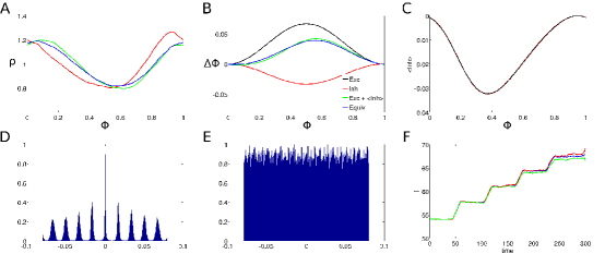
Figure 3: Performance of the 2nd and 3rd Eq. PRC versions (homogeneous inputs) with 1 ms delay. These figures compare the results of simulating an oscillator with feedforward inhibition against those of an oscillator with the equivalent PRC when the feedforward delay is 1 ms. The amplitudes for the excitatory and inhibitory PRCs are $a_{exc}=2/30$, and $a_{inh}=1/30$ respectively. The input rate is 600 Hz. A: stationary phase PDFs for the oscillator with feedforward inhibition (red), with the second version of the equivalent PRC (green), and with the third version of the equivalent PRC (blue). B: Phase resetting curves. Black=excitatory, red=inhibitory, green=second Equiv. PRC, blue=third Equiv. PRC. C: Expected value of the inhibition as a function of the phase when the initial excitatory input arrives. The red curve comes from simulating the oscillator with feedforward inhibition, and the black curve comes from the approximation in equation 26. D: Cross-correlogram between the output spike trains of the oscillators with feedforward inhibition and with the third equivalent PRC. The horizontal axis indicates time shift, and the vertical axis the normalized spike count. E: Cross-correlogram between the output spike train of the oscillator with feedforward inhibition and a spike train with constant interspike intervals and the same frequency. F: Firing rate response of the oscillators with feedforward inhibition (red), the second version of Equiv. PRC (green), and the third version of Equiv. PRC (blue) to five different levels of input rates. Input rates range from 240 Hz to 1200 Hz in constant increments of 240 Hz.

Another relevant result is in panel C of figure 3. This panel shows a close agreement between the expected inhibitory shift at time $t+d$ obtained from simulations (red curve), and from equation 26 (black curve), which approximates the expected inhibition by assuming that during the inhibitory delay all inputs will arrive at regular intervals.

Reported values of delay between an excitatory input and the corresponding feedforward inhibition are usually in the 1-2 ms range [36, 58], and have even been described as non-existent [59]. It is nevertheless relevant to test whether the formulas of this paper can be still applicable when the feedforward delay is not as short. The approaches taken here to derive the equivalent PRCs should show their shortcomings as the delay and the input firing rate are increased. With this in mind the simulations in this paper –with the exception of the one in figure 3– use a delay of 5 ms, larger than reported values, but still biologically plausible.

Figure 4 illustrates simulations done with the second and third versions of $\Delta_{eq}$ and a feedforward delay of 5 ms. It is evident in panel E that the second version of the PRC becomes incapable of matching the firing rate of the oscillator with feedforward inhibition as the input rates become larger. On the other hand, the oscillator with the third version of $\Delta_{eq}$ still displays similar behaviour to the oscillator with feedforward inhibition.

The fifth version of the equivalent PRC was also tested, using 60 different inputs, each one with different amplitudes for its excitatory and inhibitory PRCs. The result of the simulations is illustrated in figure 5. As can be seen from this figure, and from figure 4, the performance for oscillators with homogeneous and heterogeneous inputs is very similar.

Figure 4: Performance of the 2nd and 3rd Eq. PRC versions (homogeneous inputs) with 5 ms delay. Simulations for 3 different amplitude combinations of $\Delta_{exc}$ and $\Delta_{inh}$. Figures on the left correspond to $a_{exc}=1/30,\ a_{inh}=2/30$. Figures on the middle correspond to $a_{exc}=2/30,\ a_{inh}=2/30$, and Figures on the right correspond to $a_{exc}=2/30,\ a_{inh}=1/30$. The input rate for all simulations in A-D was $r=600$ Hz. Other than the input amplitudes, the only difference with the simulation of figure 3 is the delay value of 5 ms. A: stationary phase PDFs for the oscillator with feedforward inhibition (red), with the second version of the equivalent PRC (green), and with the third version of the equivalent PRC (blue). B: PRCs used in the simulation. $\Delta_{exc}$ (black), $\Delta_{inh}$ (red), second version of $\Delta_{eq}$ (green), third version of $\Delta_{eq}$ (blue). C: Expected value of the inhibition as a function of the phase when the initial excitatory input arrives. The red curve comes from simulating the oscillator with feedforward inhibition, and the black curve comes from the approximation in equation 26. D: Cross-correlogram between the output spike trains of the oscillators with feedforward inhibition and with the third equivalent PRC. The horizontal axis indicates time shift, and the vertical axis the normalized spike count. E: Firing rate response of the oscillators with feedforward inhibition (red), the second version of Equiv. PRC (green), and the third version of Equiv. PRC (blue) to five different levels of input rates. Input rates range from 240 Hz to 1200 Hz in constant increments of 240 Hz.

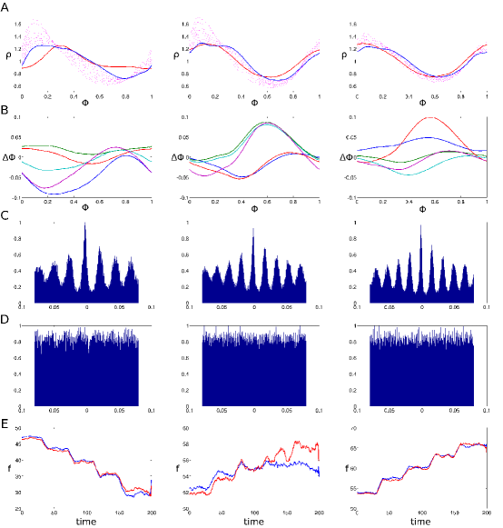
Figure 5: Performance of the fifth Eq. PRC version (heterogeneous inputs) with 5 ms delay. Simulations for 3 different combinations of mean PRC amplitudes. For each simulation a total of $N_{syn}=60$ different inputs were used, each with randomly chosen amplitudes $a_{exc}^{j}$ and $a_{inh}^{j}$ for $\Delta_{exc}^{j}$ and $\Delta_{inh}^{j}$. The firing rate for all inputs was $r_{j}=10$ Hz. Figures on the left correspond to a simulation where the mean of the PRC amplitudes is $<a_{exc}^{j}>=1/30$, $<a_{inh}^{j}>=2/30$. Figures on the middle correspond to $<a_{exc}^{j}>=2/30$, $<a_{inh}^{j}>=2/30$, and figures on the right correspond to $<a_{exc}^{j}>=2/30$, $<a_{inh}^{j}>=1/30$. A: stationary phase PDFs for the oscillator with feedforward inhibition (red), and with the fifth version of the equivalent PRCs (blue). Magenta dash-dotted lines indicate the phase PDF corresponding to intermediate iterations in the iterative procedure used. B: PRCs used in the simulation. Different colored lines show the equivalent PRCs for the first 5 synapses. C: Cross-correlogram between the output spike trains of the oscillators with feedforward inhibition and with the equivalent PRCs. The horizontal axis indicates time shift, and the vertical axis the normalized spike count. D: Cross-correlograms between the output spike train of the oscillator with feedforward inhibition and a regular spiking oscillator matching its mean frequency. E: Firing rate response of the oscillators with feedforward inhibition (red), and the equivalent PRCs (blue) to five different levels of input rates. Input rates range from 240 Hz to 1200 Hz in constant increments of 240 Hz.

3 Computational explorations of synchronization with delayed inhibition

The consequences of stochastic synchronization of Purkinje cells have not been explored before. As an initial approach to this endeavor, I explored how various factors could affect the synchrony of uncoupled oscillators receiving correlated inputs and a delayed inhibitory stimulus for each excitatory stimulus. The insight that there exists an equivalent PRC governing the response of the oscillators means that previous studies on stochastic synchronization (where each input is described with a single PRC) should be applicable in this case. As such, this exploration is guided by those studies. Stochastic synchrony is a complex and incompletely understood subject, but it is the author’s opinion that a large part of the existing results can be intuitively understood in terms of 3 factors: input correlation, heterogeneity, and PRC shape. Each of these 3 factors will be manipulated in this section. In the cases of input correlation and heterogeneity it will be shown that these factors can be manipulated without altering the PRCs (which in this case correspond to synaptic and excitability effects), but by altering instead the input sources that have a high firing rate. In this way it will be shown that different input patterns in the parallel fibers can affect the degree of synchronization in the Purkinje cells, without necessarily affecting their firing rate.

For each factor controlling stochastic synchrony, I will also mention some possible ways by which plasticity could affect it. Climbing fiber activity has been shown to mediate plasticity in several types of cerebellar cortical synapses [60], and in this paper I focus on plasticity mediated by CF activity in 3 synapse types: parallel fiber to Purkinje cell (PF-PC), molecular layer interneurons to Purkinje cells (MLI-PC), and parallel fiber to molecular layer interneurons (PF-MLI).

3.1 Details of the simulations

All simulations used 20 oscillators with frequencies drawn from a Gaussian distribution with mean of 50 Hz, and a standard deviation of 1 Hz. Each oscillator received 60 separate inputs, selected from a pool of different Poisson point processes. The effect of feedforward inhibition was simulated by applying an inhibitory input 5 ms after each excitatory input; this delay was chosen to illustrate that the effects described in this paper are present despite significant delays in the inhibition. As previously discussed, the effect of each excitatory and inhibitory input was described by separate PRCs, with excitatory PRCs being positive or null for all phases, and inhibitory PRCs being negative or null. The shape of all PRCs was the sinusoidal (positive or negative) used in the previous section. All simulations used an exact integration method, where the phases of all oscillators were updated whenever an input was received or one of them spiked.

Three different measures were used in order to test the synchrony of the 20 oscillators. The first and most significant measure was obtained by simulating a DCN neuron receiving all the spikes produced by the 20 oscillators. Neurons in the DCN tonically produce action potentials, and have powerful depolarizing currents that are triggered by hyperpolarization [25]. These features were included in a simple model of a DCN neuron consinsting of an oscillator whose frequency was raised by deep enough hyperpolarizations but relaxed back to baseline levels for moderate amounts of inhibition. The phase of the DCN neuron, represented as $\theta_{DCN}$ had an angular frequency $\omega_{DCN}$, and obeyed the equation

$$\dot{\theta}_{DCN}=\omega_{DCN}-\sum_{i}a\delta(t-t^{i})\ .$$

The value $t^{i}$ represents the arrival time of the $i$-th input, $\delta()$ is the Dirac delta function, and $a$ is a positive value representing the amplitude of the inhibitory inputs. The value $\theta_{DCN}$ is not an ordinary phase, as it is allowed to remain in the interval $[-2,1]$. Whenever the phase reaches the value 1 it is reset to the value 0, but the negative inputs can create negative values that saturate at -2. Whenever $\theta_{DCN}$ goes below the threshold value $\theta_{thr}=-0.5$ the frequency $\omega_{DCN}$ increases according to

$$\dot{\omega}_{DCN}=\frac{\omega_{max}-\omega_{DCN}}{1+e^{\xi(t_{thr}-t+t_{off})}},$$

where $\omega_{max}$ is the maximum angular frequency, $t_{thr}$ is the time when the phase last crossed the threshold, and $\xi,t_{off}$ are positive constants. On the other hand, when the frequency is above the threshold $\theta_{thr}$, $\omega_{DCN}$ obeys

$$\dot{\omega}_{DCN}=\frac{\omega_{base}-\omega_{DCN}}{1+e^{\xi(t_{thr}-t+t_{off})}},$$

where $\omega_{base}$ is the angular frequency that would take place in the absence of inputs. Notice that in the absence of threshold crossings these two equations asymptotically become $\dot{\omega}_{DCN}=\omega_{base/max}-\omega_{DCN}$. Volleys of synchronized spikes from the 20 oscillators would create deep hyperpolarizations (negative phases) in the DCN cell, and afterwards provide a time period with low inhibition, during which the DCN cell could spike. The result was that that for fixed firing rates in the input, the output firing rate of the DCN cell increased as a function of the input synchrony.

The second synchrony measure used was the circular variance [61]. In order to obtain this measure, each time one of the oscillators spiked, the phases of the other 19 oscillators were obtained. This resulted in a large sample of phases $\phi_{i}$, $i=1,\dots,N$ which should be clustered near the values 0 or 1 in the case when the oscillators spike close to one another. Since the phases are periodic, in order to average them they are represented as complex numbers with unit norm. If the number corresponding to $\phi_{i}$ is $s_{i}$, then $\mathbb{R}\{s_{i}\}=\cos(\phi_{i})$, $\mathbb{I}\{s_{i}\}=\sin(\phi_{i})$, and the average of these numbers is $\bar{s}=\frac{1}{N}\sum_{i=1}^{N}\left(\cos(\phi_{i})+i\sin(\phi_{i})\right)$. The circular variance is defined as $1-\|\bar{s}\|$.

The third synchrony measure comes from [62], and approximates the average correlation among spike trains. In short, spike trains are convolved with a Gaussian filter to obtain their continuous version, and the correlation among two spike trains comes from the normalized inner product of their continuous versions. The synchrony measure comes from the mean of these correlations for all pairs of spike trains. In the author’s implementation of this measure, due to the widths of the Gaussian filters used, the synchrony measure obtained from a group of spike trains $A$ can be compared to the synchrony of a group of spike trains $B$ only when the trains in $A$ and $B$ have similar mean firing rates.

The values for synchrony measures and average firing rates in the bar graphs of all figures come from averaging the results of 100 simulations. The simulations and all other calculations were performed in Matlab (www.mathworks.com). Source code is available upon request.

3.2 The effect of input correlation

Previous studies show that the more correlated the inputs are, the greater the potential for stochastic synchronization of their targets. In other words, for any two oscillators larger input correlations cause a peak in the distribution of their phase difference [39, 42, 49].

Figure 6: Effect of input correlation on synchrony of multiple oscillators A: (Far left) Spike raster for 100 input signals during 20 seconds of simulated time. (Middle left) excitatory connection weights from the 100 input signals to the 20 oscillators. These weights correspond to the amplitudes of the excitatory PRCs; the amplitudes of inhibitory PRCs are not shown. (Middle right) excitatory connection weights from 400 input signals to the 20 oscillators. (Far right) excitatory connection weights from 1200 input signals to the 20 oscillators in the case of uncorrelated inputs. B: DCN firing rate, circular variance, mean correlation, and Purkinje oscillator average firing rate for simulations with 3 different values for the expected number of common inputs, corresponding to connection matrices like the ones in panel A. C: Representative simulation displaying the effect of more high-frequency inputs being shared by the oscillators. (Far left) spike raster for the 500 inputs during the 3 periods of the simulation. (Middle left) excitatory connection weights. (Middle right) inhibitory connection weights. (Right) output spike train of the DCN oscillator convolved with a thin Gaussian. The red trace is a smoothing of this signal, which allows to see the fluctuations in the firing rate. D: DCN mean firing rate, circular variance, mean correlation, and Purkinje oscillator firing rate for the 3 periods shown in C, averaged over 100 simulations.

The simulation results in panels A and B of figure 6 illustrate this. There were 3 simulated trials, each one with a different level of input correlation among the 20 oscillators. In order to change the level of input correlation on each trial, the number of possible input sources (each a Poisson point process) was increased, so that with each oscillator receiving input from 60 randomly chosen sources, the expected number of common inputs decreased. The first figure in panel A of figure 6 shows the spike raster of the 100 input sources from the first trial. The other 3 figures show the amplitudes of the excitatory PRCs depending on the oscillator and the input source. An amplitude of zero (denoted by the blue color) means that the oscillator is not connected to the input source, so for each row there are 60 columns with a color other than dark blue, corresponding to values chosen randomly from a uniform distribution. This makes explicit that the expected number of common inputs among different oscillators changes between trials, from 36 to 9 to 0. In panel B it is shown that increasing input correlation increases the synchrony of the oscillators as measured by the circular variance and mean correlation described previously. The firing rate of the simulated DCN cell also increases when there are more common inputs. The figure on the far right of panel B shows that changing the number of common inputs under these conditions doesn’t have an effect on the firing rate of the oscillators.

The next simulation involving input correlation involves a single trial where the input sources have 3 different firing patterns, and is shown on panels C and D of figure 6. It is relevant to ask whether activating a particular combination of cells in the granule-cell layer could increase the response in the DCN cells of its microcomplex, not because of the average weight of their synapses onto Purkinje cells, but because they are common to many of those Purkinje cells. Mossy fiber LTP [60] promotes a population code, in which sensory stimuli can be represented by particular combinations of granule cells with a high firing rate, and Golgi feedback inhibition ensures that these combinations do not remain static [63], so a candidate code for the information in the granule cell layer could be combinations of cells spiking faster.

The simulations shown in figure 6, panels C and D have 500 inputs, and at all times half of them have a low firing rate (5 Hz), and half of them have a high firing rate (40 Hz). The PRC amplitudes for all inputs were randomly chosen from a uniform distribution in the interval [0, 0.06]. Numbering the 500 inputs, 250 are even and 250 are odd. 30 odd inputs were chosen to be received by every oscillator. For each oscillator, its remaining 30 inputs were randomly chosen from the other 470 inputs. The simulation then proceeded in 3 stages, each lasting 5 seconds. In the first stage, inputs 1 through 250 had a high firing rate, and the last 250 inputs had a low firing rate. In the second stage the 250 odd inputs had a large firing rate, and the even inputs had a low firing rate. In the third stage the last 250 inputs had a high firing rate, and the first 250 inputs had a low firing rate. The result is that the synchrony of the oscillators increased during the second stage, when the 30 common odd inputs had a high firing rate. The average firing rate of all oscillators was the same during the 3 stages.

We can ask what role plasticity could play in shaping the input correlation. The majority of PF-PC synapses seem to be silent [64, 65]. Silent synapses can become active, and active synpses can become silent [66], which suggests that Purkinje cells are continuously selecting their inputs. When there is no climbing fiber activity, sensory-evoked high-frequency input creates LTP in the PF-PC synapse [67, 68, 69, 70]. The cell seems to select those inputs that are strong and don’t happen near complex spikes. When there are complex spikes, conjunctive CF and PF activity leads to LTD in the PF-PC synapse [15, 16, 58, 17]. This is balanced with LTD in the MLI-PC synapse [58]. The cell tends to ignore inputs that happen at the time of complex spikes. This suggests that input correlation may be weakened for inputs that coincide with complex spikes. The effect of this on the DCN firing rate would be similar to the effect attributed to conjunctive LTD in the PF-PC synapse, suggesting that these two mechanisms could be complementary.

3.3 The effect of heterogeneity

Physiological heterogeneity can disrupt stochastic synchronization [54, 71, 48, 49]. This heterogeneity can present itself in the firing rates of the oscillators, and in the variety of responses to different inputs. In here I focus on the heterogeneity of responses, characterized as PRC heterogeneity.

If we have uncoupled oscillators, and the response to inputs for each one is characterized with a separate PRC, then heterogeneity in those PRCs can limit the amount of stochastic synchronization [48, 49]. Small-amplitude type II PRCs are more susceptible to this effect of heterogeneity than large-amplitude PRCs [48]. In the case of low input correlations, two heterogeneous oscillators may synchronize better than two homogeneous ones, but only in the case when the two homogeneous are “bad synchronizers,” and the heterogeneous ones include a “good synchronizer” [49]. In general, the best case for stochastic synchrony is when the PRCs are similar, and their shape is conducive to synchronization, as in the case of type II PRCs (discussed in the next subsection).

Figure 7 shows the result of a simulation in which increasing PRC homogeneity can increase oscillator synchrony and the DCN firing rate, and this is caused by shifting to a particular firing pattern of activity in the inputs. The firing pattern that increases the DCN activity does so not because it targets weaker or more inhibitory synapses, but because it targets homogeneous PRCs.

Panels A and B of figure 7 show a single representative simulation showing the effects of targeting homogeneous synapses, in a manner similar to panels C and D of figure 6. For this simulation, there is a pool of 100 possible input sources. All the odd inputs have the same excitatory and inhibitory PRC amplitudes. The even inputs have PRC amplitudes randomly chosen from a homogeneous distribution whose mean is the amplitude of odd PRCs. For the odd inputs, the excitatory and inhibitory amplitudes were chosen to be equal, because in this case the equivalent PRC has a proper shape for synchronization given the shapes and delay used (figure 4 B). Each oscillator randomly receives 30 odd and 30 even inputs. The simulation proceeds in 3 periods, each lasting 5 seconds, as was done previously. In the first period the first 50 inputs have high firing rates (40 Hz), and the last 50 inputs have low firing rates (5 Hz). During the second period the odd inputs have high firing rates, and the even inputs have low firing rates. In the last period the last 50 inputs have high firing rates, and the first 50 inputs have low firing rates. The result is that during the second period the DCN oscillator reliably increases its firing rate. The average firing rate of all Purkinje oscillators remains the same during the 3 periods, so the increase in DCN firing rate is due to an increase in synchrony. Panel B of figure 7 shows this effect for the average measures from 100 simulations.

We can also discuss the effects of plasticity on input heterogeneity, although unlike input correlation, in this case it is case it is hard to reach a hypothesis. It was mentioned in the previous subsection that high-frequency activity elicited by sensory stimulation can lead to LTP in the PF-PC synapse. Moreover, climbing fiber activity that is not paired with PF activity leads to LTP in the MLI-PC synapse, a phenomenon known as rebound potentiation [72]. The PRC amplitudes depend on the synapses, and on intrinsic excitability of the cell. Potentiation of the synapse could potentially lead to saturation in the PRC amplitudes, so that all synapses with saturated amplitudes have similar PRCs, thus decreasing heterogeneity. In the case when there is conjunctive CF-PF activity both the PF-PC and MLI-PC experience LTD. If the LTD in these two synapses is balanced, the heterogeneity could be maintained. It is thus hard to speculate whether climbing fiber activity alters the amount of heterogeneity, particularly when there are also other forms of plasticity whose effect on the shape of the effective PRC is not entirely clear.

3.4 The effect of PRC shape and amplitude

In general, most PRC shapes can produce some degree of stochastic synchrony for small correlated inputs [39, 40]. The particular shape of the PRC, however, can have a considerable effect on the degree of synchronization. Oscillators with type II PRCs, which are positive for late phases and negative for early phases [56], tend to synchronize better when receiving correlated inputs [42, 41, 48]. For small amplitude inputs the optimal shape for synchronization is a negative sinusoidal wave [44], but this shape may vary for different input amplitudes, and some shapes may be desynchronizing [46].

In the case of feedforward inhibition, the balance between excitatory and and inhibitory PRC amplitudes affects the shape of the equivalent PRC. If the excitatory and inhibitory PRCs have the same amplitude and a single peak, their equivalent PRC tends to be of type II (depending on the peak locations and the duration of the feedforward delay), and increasing this amplitude will in general be favorable for synchronization. When the excitatory and inhibitory PRCs have different amplitudes, increasing or decreasing those amplitudes in the same proportion will have an effect in the firing rate of the oscillator, so the effect of Purkinje PRC amplitude on the DCN firing rate will be largely due to changes in the firing rate of Purkinje cells.

The simulations of figure 8 are intended to illustrate how the effect of changing the PRC amplitudes depends on the shape of the equivalent PRC, which is determined by the amplitudes and shapes of the excitatory and inhibitory PRCs. The shapes of the excitatory and inhibitory PRCs are not manipulated, but the ratio of their amplitudes is set to be either 1:1, 2:1, or 1:2, which produces 3 different shapes for the equivalent PRC. For each of these 3 ratios, I run simulations for 3 different values of PRC amplitudes. Each ratio corresponds to one of the B, C, D panels, and each value of amplitude corresponds to one of the bars in the individual plots.

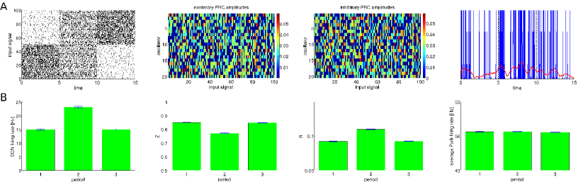
Figure 7: Effect of PRC homogeneity on synchrony of multiple oscillators. A: Representative simulation displaying the effect of homogeneous synapses being targetted by the high-frequency inputs. (Far left) spike raster for the 100 inputs during the 3 periods of the simulation. (Middle left) excitatory connection weights (PRC amplitudes). (Middle right) inhibitory connection weights. Although it is hard to appreciate in this figure, for each odd input its inhibitory and excitatory weights are the same. (Right) output spike train of the DCN oscillator convolved with a thin Gaussian. The red trace is a smoothing of this signal, which allows to see the fluctuations in the firing rate. B: DCN firing rate, circular variance, mean correlation, and average Purkinje oscillator firing rate for the 3 periods shown in C, averaged over 100 simulations.

Panel A in the first row of figure 8 shows input rasters and PRC amplitude matrices for a simulation with constant firing rates for 100 input sources. The randomly chosen amplitude matrices shown in panel A correspond to the case of balanced excitation and inhibition, and therefore these matrices are identical. In the case for the other two ratios of excitation to inhibition, the matrices are scaled versions of one another. Panel B in the second row shows the effect of changing the PRC amplitudes in the case of balanced excitation and inhibition. As can be observed, a proportional change of PRC amplitudes has a very small effect on the firing rate of the Purkinje oscillators, but the synchrony and DCN firing rate increase with the amplitude of the PRCs, as would be expected given that the shape of the equivalent PRC in this case tends to be of type II. This outcome changes when the amplitudes of excitatory PRCs are twice as large as those of the inhibitory PRCs. This case can be seen in Panel C of figure 8, where increasing the PRC amplitudes proportionally significantly increases both synchrony and Purkinje firing rate, and with these two factors opposing each other the DCN firing rate only shows a very small increase. It should be remembered that the author’s implementation of the mean correlation measure R is not a good way to compare the synchrony of different trials when they have different mean firing rates (the case in panels C and D), so the Z measure should be used instead, which shows smaller values for larger levels of synchrony. A different outcome happens when the inhibitory PRCs are twice as large as the excitatory PRCs and the amplitudes are increased while maintaining these proportions. Panel D shows that in this scenario the synchrony barely decreases as the amplitudes grow, but the Purkinje firing rates decrease significantly, resulting in an increase of the DCN firing rate. This last scenario where the synchrony’s effect is small replicates the hypothesis about the role of conjunctive LTD in the PF-PC synapse in the Marr-Albus-Ito model. To the author’s knowledge, no cerebellar model has explicitly considered the possibility of synchrony effects such as those in panels B and C.

Figure 8: Effect of PRC shape and amplitude. A: (Left) spike raster showing 100 inputs with constant firing rate; similar inputs were used for all simulations in this figure. (Center and right) PRC amplitudes for the case of balanced excitation and inhibition. Notice that amplitudes are the same for both cases. B: DCN firing rate (far left), circular variance (middle left), mean correlation (middle right), and average Purkinje oscillator firing rate (far right) for 3 different values of mean PRC amplitude in the case of balanced excitation and inhibition. C: DCN firing rate (far left), circular variance (middle left), mean correlation (middle right), and average Purkinje oscillator firing rate (far right) for 3 different values of the mean PRC amplitude in the case when excitatory PRC amplitudes are twice as large as inhibitory PRC amplitudes. D: DCN firing rate (far left), circular variance (middle left), mean correlation (middle right), and average Purkinje oscillator firing rate (far right) for 3 different values of the mean PRC amplitude in the case when inhibitory PRC amplitudes are twice as large as excitatory PRC amplitudes. The seemingly significant decrease in mean correlation as opposed to the very slight change in circular variance is an artifact of comparing the synchrony of spike trains with very different firing rates (see Materials and Methods). In this case, circular variance is the appropriate measure.

Clearly, plasticity in the synapses of Purkinje cells will have an effect on the shape and amplitude of their equivalent PRCs. The aforementioned LTP in the PF-PC synapse created by PF activity in the absence of CF activity will tend to increase the amplitude of excitatory PRCs, and rebound potentiation will create the corresponding effect for inhibitory PRCs. Conjunctive PF and CF activity will reduce both excitatory and inhibitory PRC amplitudes. The effect of this change in amplitudes will depend on a various details, such as the balance in excitation and inhibition, the shapes of the PRCs, and the importance of Purkinje cell synchrony on DCN output relative to the importance of IPSP amplitude. As long as these factors are not considered, intuitive predictions about the role of plasticity in shaping DCN output could be erroneous.

4 Discussion

I have shown that stochastic synchronization in the presence of feedforward inhibition with relatively small delays can be studied with the standard PRC methods using the equivalent PRC concept. Furthermore, I have suggested how stochastic synchronization in Purkinje cells of the cerebellum could be explored in terms of three properties: input correlation, heterogeneity (of PRCs and firing rates), and PRC shape.

4.1 Two principles for studying stochastic synchronization with delayed feedforward inhibition

There is increasing evidence for the role of synchrony in the the code of Purkinje cells’ output [73, 74]. For a long time it has been hypothesized that this synchrony arises due to mossy fiber input [75], and in the case of simple spike synchronization among Purkinje cells separated by several hundred micrometers along the direction of parallel fibers this hypothesis may be correct [76, 30, 31, 32]. Modulation of firing rates by common inputs can increase the amount of synchrony observed in a cross-correlogram, but when synchrony increases while firing rates are not being modulated, or when they are modulated in different directions, then a more complete approach to studying synchrony is required. The PRC of a cell is a compact representation of all the factors that affect its input-driven synchronization, so the application of theoretical advances in stochastic synchronization is a sensible approach to understand the effect of inputs to Purkinje cells. Studying this, however, may not be straightforward given all the connections involved in the cerebellar cortical loop. This paper suggests two principles to begin this study. A first principle is that feedforward inhibition can be conceptually removed by considering equivalent PRCs. A second principle is that synchrony is propitiated by: (i) similar firing rates in Purkinje cells, (ii) homogeneous PRCs, (iii) correlated inputs, and (iv) type II equivalent PRCs.

In theory these two principles can be experimentally tested, but some aspects appear technically challenging, such as manipulating the input correlation of Purkinje cells, or the homogeneity of their synapses. Detailed modeling is a viable alternative, although it is hampered by unknown physiological data, such as the shape and frequency dependence of inhibitory PRCs, statistical properties of some connections, or a detailed understanding of how DCN cells integrate their input. Nevertheless, there are realistic community models [77] that have approached similar challenges (e.g. [78, 38, 79, 25]), so their use along with experimental approaches is a promising future direction.

4.2 Is the PRC model adequate?

Purkinje cells are particularly complex, and their computational models tend to be mathematically intractable. The oscillator representation is a mathematically tractable model that allows to construct complicated hypotheses that may then be addressed by physiological experiments and by detailed models. This extra step in the modeling process is beneficial in the study of synchronization because the effects of changing physiological parameters are not straightforward in this case. Still, modeling Purkninje cells as oscillators and characterizing their inputs through a PRC entails a drastic reduction in complexity, which could obscure important details. Purkinje cells tonically fire simple spikes with frequencies ranging from  30 to 150 Hz; these frequencies are modulated by afferent and efferent inputs (e.g. [80, 81]), creating a wide dynamic range. Modeling and experimental results described in [82, 37], however, seem to show that the frequencies of Purkinje cells are intrinsically not so irregular, and that despite their complicated dendritic tree the summation of inputs can happen independently of their location and distribution. Indeed, the irregularity in simple spike inter-spike intervals seems to arise because of MLI inputs. Moreover, in the dendritic tree there exist voltage-gated calcium channels that amplifiy distant focal inputs more than proximal ones, canceling cable attenuation and making the somatic response largely independent of input location.

Further considerations regarding the general suitability of the PRC representation are presented in [54]. For the specific case of Purkinje cells, the main concerns when using the theory of stochastic synchronization may be the variability in firing rates, and the fact that the PRCs change depending on this firing rate. These issues are not fully resolved, but possible answers are outlined in the last subsection.

4.3 Several types of synchrony

Experimental measurements of simple-spike synchrony in Purkinje cells may point to separate mechanisms, which could depend on the distance and alignment of the cells, or on whether they depend on mossy fiber inputs.

Synchrony between PCs less than 150 micrometers apart is perhaps the most commonly found. Some of its characteristics are being present in spontaneous [75, 76, 33] and evoked activity [76], appearing in cross-correlograms as a sharp peak near zero lag on top of a peak with long tails [83, 33], or sometimes with two peaks near $\pm$5 ms [33]. The peaks seem to arise from alignment of the spikes delimiting pauses in simple spikes, and the long tails by rate modulation [83].

On the other hand, synchrony between PCs several hundred micrometers apart often happens between cells aligned in the parallel fiber direction [76, 30, 32]. The results in [31] showed more frequent synchronization along the rostrocaudal direction, possibly for cells in the same functional module. Interestingly, cells with complex spike synchrony were more likely to have synchronization of simple spikes, and there were aligned pauses (with mean duration of 129 ms, longer than the pauses of  20 ms in [83]). The results in [32] have some characteristics in common with [31], with complex spike synchronization happening orthogonally to parallel fiber beams in cells that tended to respond to the same stimuli with distances around 230 micrometers. Thus, synchrony may be found between distant PCs aligned orthogonally to the parallel fiber axis when those cells have similar response properties.

Other characteristics of the synchrony between distant PCs is that it may be observed in spontaneous activity, or may arise from inputs, and in this latter case the synchrony may not be explained by firing rate modulation [76, 30, 31]. The peak in the cross-correlogram may last for long periods, especially when afferent inputs are present [76, 30].

These data suggest that synchrony may have more than one underlying cause. Broad peaks in cross-correlograms among nearby PCs may come from comodulation; alignment of pauses could arise from a combination of common ascending axon inputs and recurrent inhibition. Synchrony between distant PCs along the parallel fiber axis presumably arises from parallel fiber interactions. Synchrony among distant PCs not aligned in the parallel fiber axis could possibly arise due to common input, but recurrent inhibition can’t be totally dismissed, although coherence in simple spike response decays with distance [33], making this less likely. The fact that for distant PCs simple spike synchronization is more likely when there is complex spike synchronization [31] suggests a learning mechanism may be in place.

4.4 Cerebellar models, firing rates, and everything else

The mechanism of stochastic synchrony does not require to assume any particular theory of cerebellar function, it merely expands the space of plausible mechanisms to implement them. There are several ways in which stochastic synchrony could be an important factor for cerebellar function, and they all depend on the physiological details. What is assumed about those details usually depends on what is assumed about the function of cerebellar microcircuitry. In this section I present some examples of synchronization playing a role in different hypotheses of cerebellar function.

We start by working under the assumption that the cerebellum is mainly involved in the control of sensory data acquisition [84]. Under this assumption, parallel fibers perform a modulatory role, and most of the evoked simple spike activity depends on ascending axons, which produce synchronous stimulation capable of making the membrane voltage cross threshold [4, 85]. Synchrony among nearby Purkinje cells can happen naturally because of the common ascending axon activation. Under these assumptions, a suggestion is that the role of parallel fibers could be to regulate the amount of synchrony that happens among the cells activated by ascending axons, and in this way allow the sensory and motor context to affect the cerebellar response. Moreover, plasticity mechanisms elicited by complex spikes could reshape the way in which these contexts affect synchrony.

In the context of the hypothesis that the cerebellum controls the acquisition of sensory information, it may be assumed that the CF-mediated plasticity acts as a homeostatic mechanism that regulates the firing rate of Purkinje cells through a negative feedback loop [86, 87]. A variation of this would be to assume that the CF-mediated plasticity also acts to equalize the simple spike firing rates of Purkinje cells, which would permit a higher degree of stochastic synchronization. A second variation could come if we assume that complex spikes serve not only a homeostatic function, but constitute a learning mechanism by firing in response to sensory stimuli which tend to require a response, such as an air puff to the eye, the stretching of a tendon, or a drop in blood pressure. In this second variation, the GC activity that tends to happen in in the absence of complex spikes in a given PC will produce strong excitatory and inhibitory synapses, whereas GC activity that tends to happen in conjunction with simple spikes will produce weak synapses. The strong, highly correlated input from the ascending axons will entrain nearby Purkinje cells as long as their subthreshold potentials remain similar, since it has a purely excitatory effect (a type I PRC). Strong and heterogeneous PF input, like the one from GC activity unrelated to complex spikes has the ability to desynchronize the phases of the subthreshold potentials, whereas the weak synapses of PF inputs correlated with complex spikes cannot disrupt the synchronization.

Indeed, when sensory evoked granule cell inputs happen in the absence of complex spikes LTP takes place in the PF-PC synapse [67, 68, 69, 70]. At the PF-MLI synapse, inputs that are not paired with CF activity can experience LTP or LTD in stellate cells, [88], and STD in basket cells [89]. Moreover, PF stimulation that is unpaired with CF activity increases the size of PC receptive fields, and the size of MLI receptive fields is decreased [90]. Finally, when there is CF activity that does not happen in conjunction with complex spikes there is an induction of LTP in the MLI-PC synapses, known as rebound potentiation [72]. These experiments suggest that the GC activity that is generally not associated with complex spike activity in a PC has strong excitatory and inhibitory synapses, large excitatory receptive fields, and a variety of responses in the PF-MLI synapse.

The opposite scenario seems to happen when GC inputs happen in conjunction with CF inputs. In this case there is LTD in both excitatory [15, 16, 58, 17] and inhibitory [58] synapses. In addition, the size of MLI receptive fields increases, while the size of PC receptive fields decreases [90]. The GC activity that is associated with complex spikes will thus tend to have weaker synapses at the Purkinje cell, and perhaps broader inhibition. If the PF activity encodes a sensory context, and if complex spikes arise in response to sensory stimuli that tend to require a response, then the contexts associated with the need for a response would be the ones that disrupt synchrony the least. An increase in synchrony for particular sensory contexts could complement effects on the firing rate of Purkinje cells, creating an output signal from cerebellar cortex that can be used both for behavior generation and as a training signal for downstream plasticity. This creates a hybrid model of cerebellar function, where there could could be control of sensory information, but this could be modulated by the particular context. In fact, there seems to be no strong a priori reason to assume that the cerebellum couldn’t perform both selection of relevant sensory information and correction of behavior execution.

A rather different hypothesis about cerebellar function comes from the view of the cerebellum as an adaptive filter (e.g. [8, 91, 10]). This view could be said to encompass the models based on the classical Marr-Albus framework [6, 7]. Typically, under this view the parallel fibers can drive the firing rate of Purkinje cells, and complex spikes signal peformance errors. The PF-PC synapses that are positively correlated with errors will undergo LTD, whereas the PF-PC signals that are negatively correlated with errors will undergo LTP, so that behavior execution is driven by the signals that minimize error. A more complete version of this hypothesis could consider the changes in synchronization that come from CF-mediated plasticity, as exemplified below.

One view of how CF-mediated plasticity could work in the Marr-Albus framework is that this plasticity increases the synchrony of the cells not correlated with complex spike activity, because of the same basic plasticity mechanisms outlined above (notice that in the previous hypothesis these mechanisms would lead to desynchronization rather than synchronization). We could assume that GC activity not associated with complex spikes produces strong excitatory and inhibitory synapses that grow until saturation, and also adopt the key assumption that when synapses grow until saturation they become homogeneous, with an equivalent PRC of type II. This would lead to a larger degree of synchrony from signals negatively correlated with complex spikes, complementing the effect of conjunctive LTD in the PF-PC synapse. On the other hand, the weak heterogeneous inputs from signals associated with complex spikes would lead to a low degree of synchronization. The dynamics of this system could correspond to a generalization of the results in [45]. In addition, the silencing of synapses from conjunctive LTD could lead to a decrease of input correlation for particular patterns of activity, as mentioned in the results section. This variation of the basic Marr-Albus-Ito hypothesis could explain to some extent the experimental results which question the sufficiency of conjunctive LTD for cerebellar learning (summarized in the introduction of this paper). For example, the deep hyperpolarizations produced by synchronous simple spikes could mediate plasticity in the targets of Purkinje cells, which would explain why the inhibition of Purkinje cells seems to be necessary for consolidation of motor learning [22].

To finish this paper, I present a general hypothesis about stochastic synchrony that is agnostic to the specific function performed by the cerebellum, but leads to different predictions to the hypotheses described above. As before, the basic idea is that stochastic synchrony is modulated in various functional modules of cerebellar cortex according to an afferent/efferent context provided by parallel fibers from other modules. An outline of how this could happen is as follows: First, afferent/efferent input increases the firing rate of Purkinje cells in one or more parasagittal cerebellar modules due to granule cell ascending axons. The firing rate modulation has a triple effect: it changes the equivalent PRC shapes for the PF inputs to type II, it increases the amplitude of those PRCs, and it equalizes the firing rates of a subset of Purkinje cells. These effects propitiate stochastic synchrony among the cells activated with similar firing rates that receive common parallel fiber input. The synchrony acts as a gain mechanism on the response of the DCN cells receiveing converging inputs from the responding Purkinje cells.

The reason why the input could change the PRC shape to type II is related to how the PRC is modulated by the cell’s firing rate. Measurement of excitatory PRCs in the Purkinje cell indicate that this curve is flat at low firing rates, but at higher firing rates it presents a peak at later phases [57]. It is not known how the inhibitory inputs change their PRC according to the firing rate, but if this PRC remains flat or develops a peak for early phases then the increase in firing rate could generate a type II PRC.

The reason why the activity produced by the ascending axons could increase the amplitude of the PRCs is because of the active channels present in the PC dendrites, combined with the fact that the synapses from the ascending axons would increase the amount of intracellular calcium. Similarly, the activity induced by the ascending axons could result in subsets of Purkinje cells with similar firing rates, which could depend on a gain modulation produced by complex spikes. Moreover, complex spikes may elicit temporary alignments of simple spike firing rates in different cells. Following a complex spike a Purkinje cell tend to go through a pause, facilitation, and suppression, and the simple spike frequency tends to be reduced [74].

The role of complex spikes under this general hypothesis of stochastic synchrony could be merely a homeostatic one, the equalization of firing rates, selection of error-reducing inputs, or the selection of inputs that predict errors or sensory events. There are assumptions which could make any of these a viable candidate, and figuring out the right ones (as well as determining whether stochastic synchrony plays a role at all in cerebellar function) will require further experimental and modeling work.

References

- [1] Ito, M.: Cerebellar circuitry as a neuronal machine. Progress in Neurobiology 78(3–5), 272–303 (2006)
- [2] Koziol, L.F., Budding, D., Andreasen, N., D’Arrigo, S., Bulgheroni, S., Imamizu, H., Ito, M., Manto, M., Marvel, C., Parker, K., Pezzulo, G., Ramnani, N., Riva, D., Schmahmann, J., Vandervert, L., Yamazaki, T.: Consensus paper: The cerebellum’s role in movement and cognition. The Cerebellum 13(1), 151–177 (2014)
- [3] Voogd, J., Glickstein, M.: The anatomy of the cerebellum. Trends in Neurosciences 21(9), 370–375 (1998)
- [4] Bower, J.M.: The organization of cerebellar cortical circuitry revisited. Annals of the New York Academy of Sciences 978(1), 135–155 (2002)
- [5] Ruigrok, T.J.H.: Ins and outs of cerebellar modules. The Cerebellum 10(3), 464–474 (2011)
- [6] Marr, D.: A theory of cerebellar cortex. The Journal of physiology 202(2), 437–470 (1969)
- [7] Albus, J.S.: A theory of cerebellar function. Mathematical Biosciences 10(1–2), 25–61 (1971)
- [8] Fujita, M.: Adaptive filter model of the cerebellum. Biological Cybernetics 45(3), 195–206 (1982)
- [9] Brunel, N., Hakim, V., Isope, P., Nadal, J.-P., Barbour, B.: Optimal information storage and the distribution of synaptic weights: Perceptron versus purkinje cell. Neuron 43(5), 745–757 (2004)
- [10] Dean, P., Porrill, J., Ekerot, C.-F., Jörntell, H.: The cerebellar microcircuit as an adaptive filter: experimental and computational evidence. Nature Reviews Neuroscience 11(1), 30–43 (2010)
- [11] Walter, J.T., Khodakhah, K.: The advantages of linear information processing for cerebellar computation. Proceedings of the National Academy of Sciences 106(11), 4471–4476 (2009)
- [12] Steuber, V., Mittmann, W., Hoebeek, F.E., Silver, R.A., De Zeeuw, C.I., Häusser, M., De Schutter, E.: Cerebellar LTD and pattern recognition by purkinje cells. Neuron 54(1), 121–136 (2007)
- [13] Yamazaki, T., Nagao, S.: A computational mechanism for unified gain and timing control in the cerebellum. PLoS ONE 7(3), 33319 (2012)
- [14] Schweighofer, N., Spoelstra, J., Arbib, M.A., Kawato, M.: Role of the cerebellum in reaching movements in humans. II. a neural model of the intermediate cerebellum. European Journal of Neuroscience 10(1), 95–105 (1998)
- [15] Ito, M., Sakurai, M., Tongroach, P.: Climbing fibre induced depression of both mossy fibre responsiveness and glutamate sensitivity of cerebellar purkinje cells. The Journal of Physiology 324(1), 113–134 (1982)
- [16] Ito, M.: Synaptic plasticity in the cerebellar cortex and its role in motor learning. The Canadian journal of neurological sciences. Le journal canadien des sciences neurologiques 20 Suppl 3, 70–74 (1993)
- [17] Hirano, T.: Long-term depression and other synaptic plasticity in the cerebellum. Proceedings of the Japan Academy. Series B, Physical and Biological Sciences 89(5), 183–195 (2013)
- [18] Welsh, J.P., Yamaguchi, H., Zeng, X.-H., Kojo, M., Nakada, Y., Takagi, A., Sugimori, M., Llinás, R.R.: Normal motor learning during pharmacological prevention of purkinje cell long-term depression. Proceedings of the National Academy of Sciences of the United States of America 102(47), 17166–17171 (2005)
- [19] Schonewille, M., Gao, Z., Boele, H.-J., Vinueza Veloz, M., Amerika, W., Šimek, A.M., De Jeu, M., Steinberg, J., Takamiya, K., Hoebeek, F., Linden, D., Huganir, R., De Zeeuw, C.: Reevaluating the role of LTD in cerebellar motor learning. Neuron 70(1), 43–50 (2011)
- [20] Miller, L.E., Holdefer, R.N., Houk, J.C.: The role of the cerebellum in modulating voluntary limb movement commands. Archives Italiennes de Biologie 140(3), 175–183 (2002)
- [21] Holdefer, R.N., Miller, L.E.: Dynamic correspondence between purkinje cell discharge and forelimb muscle activity during reaching. Brain Research 1295, 67–75 (2009)
- [22] Wulff, P., Schonewille, M., Renzi, M., Viltono, L., Sassoè-Pognetto, M., Badura, A., Gao, Z., Hoebeek, F.E., van Dorp, S., Wisden, W., Farrant, M., De Zeeuw, C.I.: Synaptic inhibition of purkinje cells mediates consolidation of vestibulo-cerebellar motor learning. Nature Neuroscience 12(8), 1042–1049 (2009)
- [23] Hoebeek, F.E., Stahl, J.S., van Alphen, A.M., Schonewille, M., Luo, C., Rutteman, M., van den Maagdenberg, A.M.J.M., Molenaar, P.C., Goossens, H.H.L.M., Frens, M.A., De Zeeuw, C.I.: Increased noise level of purkinje cell activities minimizes impact of their modulation during sensorimotor control. Neuron 45(6), 953–965 (2005)
- [24] Gauck, V., Jaeger, D.: The control of rate and timing of spikes in the deep cerebellar nuclei by inhibition. The Journal of neuroscience: the official journal of the Society for Neuroscience 20(8), 3006–3016 (2000)
- [25] Jaeger, D.: Mini-review: synaptic integration in the cerebellar nuclei–perspectives from dynamic clamp and computer simulation studies. Cerebellum (London, England) 10(4), 659–666 (2011)
- [26] Steuber, V., Schultheiss, N.W., Silver, R.A., Schutter, E.D., Jaeger, D.: Determinants of synaptic integration and heterogeneity in rebound firing explored with data-driven models of deep cerebellar nucleus cells. Journal of Computational Neuroscience 30(3), 633–658 (2011)
- [27] Person, A.L., Raman, I.M.: Purkinje neuron synchrony elicits time-locked spiking in the cerebellar nuclei. Nature 481(7382), 502–505 (2012)
- [28] MacKay, W.A., Murphy, J.T.: Integrative versus delay line characteristics of cerebellar cortex. The Canadian journal of neurological sciences. Le journal canadien des sciences neurologiques 3(2), 85–97 (1976)
- [29] Ebner, T.J., Bloedel, J.R.: Correlation between activity of purkinje cells and its modification by natural peripheral stimuli. Journal of Neurophysiology 45(5), 948–961 (1981)
- [30] Heck, D.H., Thach, W.T., Keating, J.G.: On-beam synchrony in the cerebellum as the mechanism for the timing and coordination of movement. Proceedings of the National Academy of Sciences 104(18), 7658–7663 (2007)
- [31] Wise, A.K., Cerminara, N.L., Marple-Horvat, D.E., Apps, R.: Mechanisms of synchronous activity in cerebellar purkinje cells. The Journal of Physiology 588(13), 2373–2390 (2010)
- [32] Bosman, L.W.J., Koekkoek, S.K.E., Shapiro, J., Rijken, B.F.M., Zandstra, F., van der Ende, B., Owens, C.B., Potters, J.-W., de Gruijl, J.R., Ruigrok, T.J.H., De Zeeuw, C.I.: Encoding of whisker input by cerebellar purkinje cells. The Journal of Physiology 588(Pt 19), 3757–3783 (2010)
- [33] de Solages, C., Szapiro, G., Brunel, N., Hakim, V., Isope, P., Buisseret, P., Rousseau, C., Barbour, B., Léna, C.: High-frequency organization and synchrony of activity in the purkinje cell layer of the cerebellum. Neuron 58(5), 775–788 (2008)
- [34] Pikovsky, A.: Synchronization: A Universal Concept in Nonlinear Sciences. Cambridge University Press, ??? (2003)
- [35] Teramae, J.-n., Tanaka, D.: Robustness of the noise-induced phase synchronization in a general class of limit cycle oscillators. Physical Review Letters 93(20), 204103 (2004)
- [36] Mittmann, W., Koch, U., Häusser, M.: Feed-forward inhibition shapes the spike output of cerebellar purkinje cells. The Journal of physiology 563(Pt 2), 369–378 (2005)
- [37] De Schutter, E.: Using realistic models to study synaptic integration in cerebellar purkinje cells. Reviews in the neurosciences 10(3-4), 233–245 (1999)
- [38] Santamaria, F., Tripp, P.G., Bower, J.M.: Feedforward inhibition controls the spread of granule cell–induced purkinje cell activity in the cerebellar cortex. Journal of Neurophysiology 97(1), 248–263 (2007)
- [39] Nakao, H., Arai, K.-s., Nagai, K., Tsubo, Y., Kuramoto, Y.: Synchrony of limit-cycle oscillators induced by random external impulses. Physical Review E 72(2), 026220 (2005)
- [40] Nakao, H., Arai, K., Kawamura, Y.: Noise-induced synchronization and clustering in ensembles of uncoupled limit-cycle oscillators. Physical Review Letters 98(18), 184101 (2007)
- [41] Galán, R.F., Ermentrout, G.B., Urban, N.N.: Stochastic dynamics of uncoupled neural oscillators: Fokker-planck studies with the finite element method. Physical Review E 76(5), 056110 (2007)
- [42] Marella, S., Ermentrout, G.B.: Class-II neurons display a higher degree of stochastic synchronization than class-i neurons. Physical Review E 77(4), 041918 (2008)
- [43] Arai, K., Nakao, H.: Phase coherence in an ensemble of uncoupled limit-cycle oscillators receiving common poisson impulses. Physical Review E 77(3), 036218 (2008)
- [44] Abouzeid, A., Ermentrout, B.: Type-II phase resetting curve is optimal for stochastic synchrony. Physical Review E 80(1), 011911 (2009)
- [45] Ly, C., Ermentrout, G.B.: Synchronization dynamics of two coupled neural oscillators receiving shared and unshared noisy stimuli. Journal of Computational Neuroscience 26(3), 425–443 (2009)
- [46] Hata, S., Arai, K., Galán, R.F., Nakao, H.: Optimal phase response curves for stochastic synchronization of limit-cycle oscillators by common poisson noise. Physical Review E 84(1), 016229 (2011)
- [47] Bressloff, P.C., Lai, Y.M.: Stochastic synchronization of neuronal populations with intrinsic and extrinsic noise. Journal of mathematical neuroscience 1(1), 2 (2011)
- [48] Burton, S.D., Ermentrout, G.B., Urban, N.N.: Intrinsic heterogeneity in oscillatory dynamics limits correlation-induced neural synchronization. Journal of Neurophysiology 108(8), 2115–2133 (2012)
- [49] Zhou, P., Burton, S.D., Urban, N.N., Ermentrout, G.B.: Impact of neuronal heterogeneity on correlated colored noise-induced synchronization. Frontiers in Computational Neuroscience 7 (2013)
- [50] Kurebayashi, W., Shirasaka, S., Nakao, H.: Phase reduction method for strongly perturbed limit cycle oscillators. Physical Review Letters 111(21), 214101 (2013)
- [51] Winfree, A.T.: The Geometry of Biological Time. Springer, ??? (2001)
- [52] Kuramoto, Y.: Chemical Oscillations, Waves, and Turbulence. Courier Dover Publications, ??? (1984)
- [53] Schultheiss, N.W., Prinz, A.A., Butera, R.J. (eds.): Phase Response Curves in Neuroscience: Theory, Experiment, and Analysis. Springer series in computational neuroscience, vol. v. 6. Springer, New York (2012)
- [54] Smeal, R.M., Ermentrout, G.B., White, J.A.: Phase-response curves and synchronized neural networks. Philosophical Transactions of the Royal Society B: Biological Sciences 365(1551), 2407–2422 (2010)
- [55] Lasota, A., Mackey, M.C.: Probabilistic Properties of Deterministic Systems. Cambridge University Press, ??? (2008)
- [56] Hansel, D., Mato, G., Meunier, C.: Synchrony in excitatory neural networks. Neural Computation 7(2), 307–337 (1995)
- [57] Phoka, E., Cuntz, H., Roth, A., Häusser, M.: A new approach for determining phase response curves reveals that purkinje cells can act as perfect integrators. PLoS Comput Biol 6(4), 1000768 (2010)
- [58] Mittmann, W., Häusser, M.: Linking synaptic plasticity and spike output at excitatory and inhibitory synapses onto cerebellar purkinje cells. The Journal of Neuroscience 27(21), 5559–5570 (2007)
- [59] Blot, A., Barbour, B.: Ultra-rapid axon-axon ephaptic inhibition of cerebellar purkinje cells by the pinceau. Nature neuroscience 17(2), 289–295 (2014)
- [60] Hansel, C., Linden, D.J., D’Angelo, E.: Beyond parallel fiber LTD: the diversity of synaptic and non-synaptic plasticity in the cerebellum. Nature Neuroscience 4(5), 467–475 (2001)
- [61] Allen, F.H., Johnson, O.: Automated conformational analysis from crystallographic data. 4. statistical descriptors for a distribution of torsion angles. Acta Crystallographica Section B Structural Science 47(1), 62–67 (1991)
- [62] Schreiber, S., Fellous, J.M., Whitmer, D., Tiesinga, P., Sejnowski, T.J.: A new correlation-based measure of spike timing reliability. Neurocomputing 52-54, 925–931 (2003)
- [63] D’Angelo, E., De Zeeuw, C.I.: Timing and plasticity in the cerebellum: focus on the granular layer. Trends in Neurosciences 32(1), 30–40 (2009)
- [64] Isope, P., Barbour, B.: Properties of unitary granule cell→purkinje cell synapses in adult rat cerebellar slices. The Journal of Neuroscience 22(22), 9668–9678 (2002)
- [65] Wang, S.S.-H., Khiroug, L., Augustine, G.J.: Quantification of spread of cerebellar long-term depression with chemical two-photon uncaging of glutamate. Proceedings of the National Academy of Sciences 97(15), 8635–8640 (2000)
- [66] Ekerot, C.-F., Jömtell, H.: Parallel fiber receptive fields: a key to understanding cerebellar operation and learning. The Cerebellum 2(2), 101–109 (2003)
- [67] Lev-Ram, V., Wong, S.T., Storm, D.R., Tsien, R.Y.: A new form of cerebellar long-term potentiation is postsynaptic and depends on nitric oxide but not cAMP. Proceedings of the National Academy of Sciences 99(12), 8389–8393 (2002)
- [68] Coesmans, M., Weber, J.T., De Zeeuw, C.I., Hansel, C.: Bidirectional parallel fiber plasticity in the cerebellum under climbing fiber control. Neuron 44(4), 691–700 (2004)
- [69] Wang, X., Chen, G., Gao, W., Ebner, T.: Long-term potentiation of the responses to parallel fiber stimulation in mouse cerebellar cortex in vivo. Neuroscience 162(3), 713–722 (2009)
- [70] Schonewille, M., Belmeguenai, A., Koekkoek, S.K., Houtman, S.H., Boele, H.J., van Beugen, B.J., Gao, Z., Badura, A., Ohtsuki, G., Amerika, W.E., Hosy, E., Hoebeek, F.E., Elgersma, Y., Hansel, C., De Zeeuw, C.I.: Purkinje cell-specific knockout of the protein phosphatase PP2b impairs potentiation and cerebellar motor learning. Neuron 67(4), 618–628 (2010)
- [71] Markowitz, D.A., Collman, F., Brody, C.D., Hopfield, J.J., Tank, D.W.: Rate-specific synchrony: Using noisy oscillations to detect equally active neurons. Proceedings of the National Academy of Sciences 105(24), 8422–8427 (2008)
- [72] Kano, M., Rexhausen, U., Dreessen, J., Konnerth, A.: Synaptic excitation produces a long-lasting rebound potentiation of inhibitory synaptic signals in cerebellar purkinje cells. Nature 356(6370), 601–604 (1992)
- [73] Person, A.L., Raman, I.M.: Synchrony and neural coding in cerebellar circuits. Frontiers in Neural Circuits 6, 97 (2012)
- [74] De Zeeuw, C.I., Hoebeek, F.E., Bosman, L.W.J., Schonewille, M., Witter, L., Koekkoek, S.K.: Spatiotemporal firing patterns in the cerebellum. Nature Reviews Neuroscience 12(6), 327–344 (2011)
- [75] Bell, C.C., Grimm, R.J.: Discharge properties of purkinje cells recorded on single and double microelectrodes. Journal of Neurophysiology 32(6), 1044–1055 (1969)
- [76] Ebner, T.J., Bloedel, J.R.: Temporal patterning in simple spike discharge of purkinje cells and its relationship to climbing fiber activity. Journal of Neurophysiology 45(5), 933–947 (1981)
- [77] Bower, J.M.: The emergence of community models in computational neuroscience: The 40-year history of the cerebellar purkinje cell. In: Bower, J.M. (ed.) 20 Years of Computational Neuroscience. Springer Series in Computational Neuroscience, pp. 103–140. Springer, ??? (2013). http://link.springer.com/chapter/10.1007/978-1-4614-1424-7_5
- [78] Jaeger, D.: No parallel fiber volleys in the cerebellar cortex: Evidence from cross-correlation analysis between purkinje cells in a computer model and in recordings from anesthetized rats. Journal of Computational Neuroscience 14(3), 311–327 (2003)
- [79] Sudhakar, S.K., De Schutter, E.: A biophysical model of cerebellar molecular layer interneuron. BMC Neuroscience 14(Suppl 1), 96 (2013)
- [80] Holtzman, T., Rajapaksa, T., Mostofi, A., Edgley, S.A.: Different responses of rat cerebellar purkinje cells and golgi cells evoked by widespread convergent sensory inputs. The Journal of Physiology 574(2), 491–507 (2006)
- [81] Holdefer, R.N., Miller, L.E.: Dynamic correspondence between purkinje cell discharge and forelimb muscle activity during reaching. Brain Research 1295, 67–75 (2009)
- [82] De Schutter, E., Bower, J.M.: Simulated responses of cerebellar purkinje cells are independent of the dendritic location of granule cell synaptic inputs. Proceedings of the National Academy of Sciences of the United States of America 91(11), 4736–4740 (1994)
- [83] Shin, S.-L., Schutter, E.D.: Dynamic synchronization of purkinje cell simple spikes. Journal of Neurophysiology 96(6), 3485–3491 (2006)
- [84] Bower, J.M.: Is the cerebellum sensory for motor’s sake, or motor for sensory’s sake: the view from the whiskers of a rat? Progress in brain research 114, 463–496 (1997)
- [85] Santamaria, F., Jaeger, D., Schutter, E.D., Bower, J.M.: Modulatory effects of parallel fiber and molecular layer interneuron synaptic activity on purkinje cell responses to ascending segment input: A modeling study. Journal of Computational Neuroscience 13(3), 217–235 (2002)
- [86] De Schutter, E.: Cerebellar long-term depression might normalize excitation of purkinje cells: a hypothesis. Trends in Neurosciences 18(7), 291–295 (1995)
- [87] Bengtsson, F., Hesslow, G.: Cerebellar control of the inferior olive. The Cerebellum 5(1), 7–14 (2006)
- [88] Rancillac, A., Crepel, F.: Synapses between parallel fibres and stellate cells express long-term changes in synaptic efficacy in rat cerebellum. The Journal of Physiology 554(Pt 3), 707–720 (2004)
- [89] Bao, J., Reim, K., Sakaba, T.: Target-dependent feedforward inhibition mediated by short-term synaptic plasticity in the cerebellum. The Journal of neuroscience: the official journal of the Society for Neuroscience 30(24), 8171–8179 (2010)
- [90] Jörntell, H., Ekerot, C.-F.: Reciprocal bidirectional plasticity of parallel fiber receptive fields in cerebellar purkinje cells and their afferent interneurons. Neuron 34(5), 797–806 (2002)
- [91] Thach, W.T.: What is the role of the cerebellum in motor learning and cognition? Trends in Cognitive Sciences 2(9), 331–337 (1998)