Supersolar metallicity in G0–G3 main sequence stars with V$<$15

Abstract

The basic stellar atmospheric parameters (effective temperature, surface gravity and global metallicity) were simultaneously determined for a sample of 233 stars, limited in magnitude ($V$ $<$15) with spectral types between G0 and G3 and luminosity class V (main sequence). The analysis was based on spectroscopic observations collected at the Observatorio Astrofísico Guillermo Haro and using a set of Lick-like indices defined in the spectral range of 3800–4800 Å. An extensive set of indices computed in a grid of theoretical spectra was used as a comparison tool in order to determine the photospheric parameters. The method was validated by matching the results from spectra of the asteroids Vesta and Ceres with the Sun parameters. The main results were: i) the photospheric parameters were determined for the first time for 213 objects in our sample; ii) a sample of 20 new super metal-rich stars candidates was found.

1 Introduction

Stellar atmospheric parameters are of fundamental importance in a plethora of astrophysical scenarios. On the one hand, effective temperature and surface gravity ($T_{\rm eff}$ and $\log{g}$) and, to some extent, chemical composition allow, for instance, to properly locate stars in the HR diagram and therefore to better establish their evolutionary status and ages. This has been particularly true for segregating stars on the main sequence from evolved objects in the Kepler field in a wide temperature range (Molenda-Żakowicz et al., 2013). They are also important in identifying solar analogues or twins that permit to place our Sun into context of its neighbourhood (Porto de Mello et al., 2014).
On the other hand, the stellar chemical composition turns out to be a primary criterion in the analysis of the chemical history of galaxies, including our Milky Way. Global metallicity ([M/H]) provides, in the case of metal-poor stars, information on the early stages of galaxy evolution, before the rapid insertion of enriched yields through supernovae events shaped their observable chemical properties. Less attention, however, was initially paid to the super metal-rich (SMR) stars, in spite of having been defined more than four decades ago by Spinrad & Taylor (1969) as stars with metallicity higher than the Hyades. This leading (and controversial) study and that of Rich (1988) on the galactic bulge have for a long time served as the basis for investigations of metal-rich extragalactic populations, such as those found in elliptical galaxies and spheroidal components (mainly bulges) of spirals. In this work, we adopt a threshold of +0.16 dex for a star to be considered SMR; this value is slightly more conservative than the recent estimate of the average metallicity of the Hyades ([Fe/H]=0.13$\pm$0.06 dex), reported by Heiter et al. (2014)
More locally, SMR stars have become particularly interesting objects in view of the well established correlation between the presence of giant exoplanets and the stellar metal content (Gonzalez, 1998; Santos et al., 2001; Fischer & Valenti, 2005). Such correlation indicates that the probablility of finding a giant planet significantly increases with increasing metallicity. It is now known that 25% of metal-rich nearby field stars harbor planets, while the prevalence is reduced to 3% if we consider solar abundances (Santos, 2008). The metallicity-planet correlation has posed interesting challenges to the current planet formation scenarios, since it appears to favour the core accretion model (Alibert, Mordasini & Benz, 2004) over the planetary formation as a result of disk instabilities (Boss, 1997). It has also motivated a number of studies in search for giant exoplanets in field stars as well as in metal-rich stellar clusters as NGC 6791 (Bruntt et al., 2003).

To date, SMR stars are attractive on both of the above scenarios, and studies in one field have been shared by the other. For instance, the construction of stellar databases as tools for the synthesis of stellar population have recently been incorporated in exoplanetary studies (Buzzoni et al., 2001). Conversely, stellar studies, aimed at finding fiducial targets for exoplanet searches and potential correlations between stellar host properties and the presence of substellar companions, have already impacted broader issues, as the chemical evolution of the Milky Way (see Neves et al., 2009; Adibekyan et al., 2011, 2012, and references therein).

In this work, we carried out a spectroscopic analysis of a sample of stars of spectral types G0–G3, luminosity class V, in the visual magnitude interval $4.05<V<14.77$, that has been observed at moderate resolution (FWHM 2.5 Å). We simultaneously derive the three leading atmospheric parameters ($T_{\rm eff}$, $\log{g}$ and [M/H]), through the study of their spectroscopic indices, and identify a new sample of SMR stars as potential targets of planet searches.

2 Stellar sample and observations

We selected in late 2008 a sample of stars from SIMBAD database using the following criteria: i) spectral type between G0 and G3; ii) luminosity class V; iii) visible magnitude $V$ $<$15 mag; and iv) declination $\delta>-10\degr$. The selection resulted in about 1200 objects. We report here the results for 233 stars. We carried out the spectroscopic observations at the 2.12 meter telescope of the Observatorio Astrofísico Guillermo Haro (Sonora, Mexico) between 2008 and 2013, with a Boller & Chivens spectrograph, equipped with a Versarray 1300$\times$1340 CCD. The grating of 600 l/mm and the slit width of 200 $\mu$m provided a constant spectral resolution of 2.5 Å FWHM and a dispersion of 0.7 Å px^-1 along the wavelength range between about 3800 and 4800 Å. Typically, we acquired 2 or more images for each star, with total exposure times between 3 min, for the brighter objects, and about 60 min for the fainter ones, to reach a signal-to-noise ratio per pixel (S/N) of 30–80, computed in a window of 100 Å around 4600 Å. The sample is presented in Table 1, where we list the star identification, the $V$ magnitude and the spectral type as given in SIMBAD. In Fig. 1 we show the distribution of the $V$ magnitude for the stars in our sample.

In addition to the sample described above, we also observed a set of 29 reference stars from the PASTEL catalogue (Soubiran et al., 2010) and complemented this sample with 35 objects from Liu et al. (2008). The reference sample will serve to test the adequacy of theoretical spectra in a range of atmospheric parameters, as explained in Sect. 4.1. The main photospheric parameters (see Table 2) of these objects were obtained by averaging only those PASTEL entries that provide the three parameters ($T_{\rm eff}$,$\log{g}$,[M/H]) to minimize the effect of degeneracies. The reference stars span 4857–6987 K in effective temperature, 3.00–4.68 dex in surface gravity and -1.43 – +0.30 dex in global metallicity.

Table 1: The sample of the observed stars. The full table is available in the electronic version.

Name	V (mag)	Spectral type
HD 236373	10.22	G0V
1RXS J003845.9+332534	10.33	G2V
[BHG88] 40 1943	14.77	G2V
HD 4602	9.04	G0V
BD+59 140	10.37	G2V
TYC 4497-874-1	10.92	G3V
HD 5649	8.70	G0V
TYC 4017-1351-1	11.22	G0V
BD+60 167	10.34	G0V
BD+02 189	10.29	G1V

Figure 1: Distribution of V magnitude for all the sample.

Table 2: The atmospheric parameters for the 64 reference stars.

Star	$T_{\rm eff}$	$\log{g}$	[M/H]	Star	$T_{\rm eff}$	$\log{g}$	[M/H]	Star	$T_{\rm eff}$	$\log{g}$	[M/H]
	(K)	(dex)	(dex)		(K)	(dex)	(dex)		(K)	(dex)	(dex)
HD3651	5205	4.49	0.10	HD99285	6599	3.84	-0.22	HD134083	6537	4.31	0.02
HD3765	5034	4.53	0.05	HD100180	5927	4.25	-0.06	HD134113	5680	4.06	-0.78
HD15335	5858	3.93	-0.18	HD100563	6401	4.31	0.05	HD136064	6121	4.03	-0.03
HD18757	5685	4.36	-0.29	HD101606	6134	3.98	-0.75	HD137052	6423	3.94	-0.09
HD18803	5658	4.46	0.13	HD102574	6030	3.92	0.16	HD139457	5954	4.05	-0.51
HD25621	6251	3.95	0.01	HD106156	5464	4.68	0.18	HD142357	6475	3.44	-0.02
HD28271	6160	3.85	-0.10	HD114606	5610	4.28	-0.48	HD142860	6286	4.14	-0.20
HD29645	5985	4.04	0.06	HD117176	5527	3.95	-0.06	HD144284	6309	4.13	0.20
HD33256	6242	3.99	-0.36	HD117361	6789	3.95	-0.27	HD145976	6720	4.10	0.01
HD33608	6489	4.08	0.22	HD120136	6445	4.30	0.27	HD149414	5055	4.40	-1.31
HD35984	6175	3.68	-0.07	HD122742	5509	4.39	0.00	HD149996	5662	4.10	-0.53
HD43386	6480	4.27	-0.06	HD125184	5659	4.11	0.27	HD150012	6380	3.80	0.05
HD61295	6987	3.05	0.25	HD126512	5758	4.05	-0.62	HD150177	6096	3.95	-0.58
HD67228	5814	4.00	0.11	HD126660	6322	4.27	-0.04	HD155646	6180	3.84	-0.13
HD76292	6866	3.77	-0.22	HD126681	5522	4.58	-1.18	HD157373	6427	4.08	-0.43
HD87646	5961	4.41	0.30	HD127334	5651	4.15	0.18	HD157856	6309	3.93	-0.18
HD87822	6597	4.10	0.17	HD128167	6712	4.32	-0.37	HD159332	6184	3.85	-0.23
HD88986	5827	4.13	0.03	HD128959	5478	3.00	-0.92	HD185144	5268	4.49	-0.23
HD91752	6423	4.03	-0.25	HD130087	6040	4.34	0.26	HD190228	5306	3.83	-0.26
HD94028	5963	4.13	-1.43	HD130945	6431	4.06	0.06	HD222404	4857	3.23	0.09
HD95128	5861	4.30	0.00	HD131156	5457	4.52	-0.14
HD99028	6739	3.98	0.06	HD132375	6273	4.16	0.01

Since we know with great accuracy the photospheric parameters of the Sun, we also observed, in February 2013, its spectrum reflected by the asteroids Vesta and Ceres, using the same observational set-up and a CCD600 camera which provides a slightly larger dispersion of 1.0 Å pixel^-1. At the time of the observation, they had V=7.71 and 8.05 mag, respectively. We took five exposures of each target, for a total of 780 and 750 seconds, respectively, providing S/N$\sim$60.

The data were reduced following the standard procedure in IRAF: bias subtraction, flat field correction, cosmic ray removal, wavelength calibration (by means of an internal HeAr lamp), and flux calibration (using spectrophotometric standard stars from the ESO list. We then shifted all spectra to the rest frame, using an average radial velocity obtained from measuring the shift of several absorption lines along each spectrum. Finally, for each star we co-added its multiple spectra, weighted by their mean S/N. We show the spectral energy distributions (SEDs) of Vesta and Ceres in Fig 2, while in Fig. 3 we present the spectra of some representative objects.

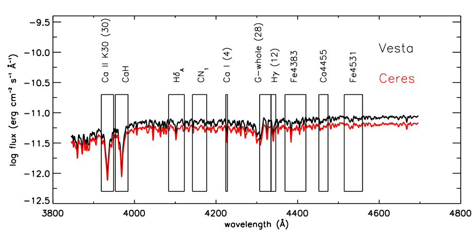
Figure 2: Solar SED from the observations of the asteroids Vesta (black, upper spectrum) and Ceres (red, low spectrum). The rectangles represent the central bands of the 10 indices of Table 3.

Figure 3: SEDs of an illustrative sub-set of stars in our sample.

3 The library of synthetic stellar spectra

With the goal of determining the atmospheric parameters of the target stars, we need a theoretical counterpart. We adopted the library of high spectral resolution SEDs of Munari et al. (2005), which is based on the ATLAS model atmospheres of Castelli & Kurucz (2003) and covers the 2500–10500 Å wavelength range. Bertone et al. (2004) showed that ATLAS theoretical SEDs (Kurucz, 1993; Castelli & Kurucz, 2003) are suitable to match the spectra of G-type stars, more so when the line blending at the spectral resolution of our observations dilutes the potential inconsintencies that might be present in individual lines (Bertone et al., 2008). From the whole collection of Munari et al. (2005) SEDs, we extracted a subset of SEDs, hereafter called the Munari’s library, using the following criteria: resolving power $R=20\,000$, $4750\leq T_{\rm eff}\leq 7000$ K, $3.0\leq\log{g}\leq 5.0$ dex, $-2.5\leq\rm{[M/H]}\leq 0.5$ dex, solar-scaled abundances, microturbulence $\xi=2$ km s^-1, and rotational velocity $V_{\rm rot}=0$ km s^-1. We then degraded all the SEDs to match the observational spectral resolution with a Gaussian convolution.

4 The spectroscopic indices

In order to quantify the flux absorption of the most relevant spectral features, we considered the 41 spectral indices defined in the works of Worthey & Ottaviani (1997), Trager et al. (1998), Carretero (2007), and Lee et al. (2008) that fall within the spectral range of the observations. These indices are constructed with 3 wavelength bands: a central one, that includes the selected spectral feature, and two side bands, conveniently placed where the line blanketing is minimum, that are used to define a pseudo-continuum level. For the sake of homogeneity, we computed the values $I$ of all indices following the definition of the Lick/IDS system (Trager et al., 1998). The integrated fluxes within the side bands provide, through a linear fit, the pseudo-continuum level for the central band. The index is obtained from

$$I=\int_{\lambda_{1}}^{\lambda_{2}}\left(1-\frac{F_{\rm cb}(\lambda)}{F_{c}(\lambda)}\right)d\lambda\,,$$ (1)

where $F_{\rm cb}$ is the flux in the central band, whose wavelength limits are $\lambda_{1}$ and $\lambda_{2}$, and $F_{\rm c}$ is the flux of the pseudo-continuum at the central band. All results are therefore given as a pseudo-equivalent width in angstroms.

We computed the full set of indices for all the observed stars and the synthetic SEDs of the Munari’s library. However, we made use of only 10 indices to determine the stellar parameters. We selected these 10 indices as the most promising for the determination of atmospheric parameters, as described in Sect. 4.2. We report the definition of the wavelength bands of these indices in Table 3, along with their typical error (see Sect. 4.2).

Table 3: Wavelength band definition for 10 spectroscopic indices. Last column provides that reference where the index was defined: S = Lee et al. (2008), L = Trager et al. (1998), W = Worthey & Ottaviani (1997) y C = Carretero (2007).

Name	Central Band	Blue Band	Red Band	$\bar{\sigma_{I}}$	Ref.
	$\lambda$ (Å)	$\lambda$ (Å)	$\lambda$ (Å)	(Å)
Ca II K30 (30)	3918.600 - 3948.600	3907.500 - 3912.500	4007.500 - 4012.500	0.18	S
CaH	3953.000 - 3984.200	3890.300 - 3913.100	4008.700 - 4029.200	0.14	C
H$\delta_{A}$	4083.500 - 4122.250	4041.600 - 4079.750	4128.500 - 4161.000	0.15	W
CN1	4142.125 - 4177.125	4080.125 - 4117.625	4244.125 - 4284.125	0.15	L
Ca I (4)	4224.000 - 4228.000	4208.000 - 4214.000	4230.000 - 4234.000	0.04	S
G-whole (28)	4307.000 - 4335.000	4090.000 - 4102.000	4500.000 - 4514.000	0.13	S
H$\gamma$ (12)	4334.500 - 4346.500	4247.000 - 4267.000	4415.000 - 4435.000	0.07	S
Fe4383	4369.125 - 4420.375	4359.125 - 4370.375	4442.875 - 4455.375	0.23	L
Ca4455	4452.125 - 4474.625	4445.875 - 4454.625	4477.125 - 4492.125	0.11	L
Fe4531	4514.250 - 4559.250	4504.250 - 4514.250	4560.500 - 4579.250	0.18	L

4.1 Transformation of the indices to the observational system

Theoretical spectra do not perfectly reproduce the observations (e.g. Bertone et al., 2004, 2008; Coelho, 2014), as they are affected by systematic effects (physical and geometrical approximations, inaccurate atomic parameters for opacity computation, etc.). Therefore, we must first transform the theoretical indices from the Munari’s library to the observational system by using the set of reference stars. For each of the these objects, we made a trilinear interpolation in the ($T_{\rm eff}$, $\log{g}$, [M/H]) parameter space to produce its synthetic spectrum. Then, for each index, we carried out a least square linear fitting of the synthetic vs. observed indices of the reference stars to transform the theoretical indices as:

$$I_{\rm{teo,cal}}=\frac{I_{\rm teo}-b}{m}\,,$$ (2)

where $I_{\rm{teo,cal}}$ is the calibrated theoretical index, I_teo is the original theoretical index, and $b$ and $m$ are the y-intercept and slope of the linear fitting. To exclude unreliable outliers, we adopted an iterative 3$\sigma$ clipping method.

4.2 Selection and properties of the set of suitable indices

In order to obtain the most accurate and precise photospheric parameters, we carried out a meticulous index selection to extract, from the pool of 41 indices, those that generate a good degree of “orthogonality” in the ($T_{\rm eff}$, $\log{g}$, [M/H]) parameter space and that are relatively well reproduced by the uncalibrated theoretical values. We realized that the inclusion of inadequate indices affects both accuracy and precision of the results.

The first step in the process was to select only those indices with slopes $0.6<m<1.4$ of the calibration equation, so to immediately discard the less reliable indices. Several indices measure the same spectral feature, but with different definitions of the three wavelength bands. In those cases, we picked up just one index, based on the visual inspection of the behaviour of the indices against variations in $T_{\rm eff}$, $\log{g}$ and [M/H]: for instance, in the case of the Balmer H$\delta$ line, we chose the index that maximized the sensitivity to temperature, while minimized the dependence on surface gravity and metallicity. Finally, we used the observed solar spectra that we collected from Vesta and Ceres as a test bench. We considered many combinations of the sub-set of indices selected at this point and we performed a chi-square analysis to determine the photospheric parameters of the Sun, by comparing the observed and calibrated theoretical indices, and we chose the combination that provided the best match with the accepted parameters of the Sun ($T_{\rm eff}$, $\log{g}$, [M/H])=(5777 K, 4.44, 0.0). The best result was given by the set of the following 10 indices: Ca II K30 (30), CaH, H$\delta_{\rm A}$, CN₁, Ca I (4), G-whole (28), H$\gamma$ (12), Fe4383, Ca4455, and Fe4531; they yielded, for both spectra, ($T_{\rm eff}$, $\log{g}$, [M/H])= (5750,4.50,-0.02).

For this set of indices, we present in Fig. 4 the plots of the theoretical vs. observed indices for the reference stars, along with the linear best fit, from which we derived the transformation equation, whose $b$ and $m$ parameters are given in Table 4. The two Balmer line indices and Fe4383 are already very well reproduced by the synthetic Munari’s spectra. The other indices need a larger correction to match the observations. In several cases, the linear fit crosses the bisector: this indicates that there exists a combination of photospheric parameters for which the theoretical index matches the observed one. However, these combinations strongly vary from index to index, revealing that different spectral regions (or element opacity) are better reproduced at different, for instance, $T_{\rm eff}$.

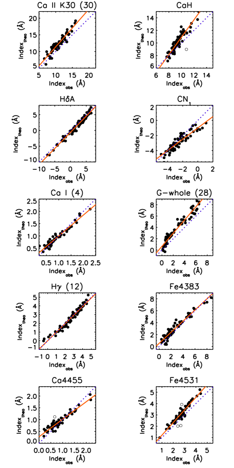
Figure 4: Theoretical vs. observed indices for the set of reference stars for the selected set of indices. The dotted line indicates the bisector of the plane, while the solid line shows the best linear fit of the data. The open dots are the data rejected by 3$\sigma$ clipping.

Table 4: The slope, y-intercept, standard error between the fit and the observational data, and the number of stars rejected in the 3-$\sigma$ clipping method are of the best linear fit.

Index	$m$	$b$	$\sigma$	r3σ
Ca II K30 (30)	1.134	0.043	0.857	0
CaH	1.387	-2.963	0.578	1
H$\delta_{A}$	1.026	-0.599	0.627	0
CN1	0.749	-1.001	0.465	0
Ca I (4)	0.848	0.154	0.090	0
G-whole (28)	1.164	0.646	0.630	0
H$\gamma$ (12)	0.980	0.013	0.284	0
Fe4383	0.930	0.543	0.484	0
Ca4455	0.741	0.276	0.099	1
Fe4531	1.115	0.097	0.206	3

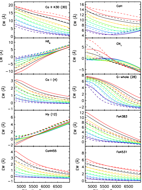
Figure 5: Indices values as a function of stellar parameters. In each panel the surface gravity is fixed at the values $\log g$ = 3.0 (dashed lines) and 5.0 dex (solid lines). Different colours represent different metallicities, from [M/H] = -2.5 dex (purple) to 0.5 dex (red), with a step of 0.5 dex.

The transformed theoretical indices as a function of the three atmospheric parameters are depicted in Fig. 5, however, in order to understand how significant is the sensitivity of each index versus these parameters, we can compare its dynamical range with a typical error. We estimated this error with a Montecarlo method: we assumed a S/N = 50 at 4660 Å, where the line blanketing is minimum, to simulate a photometric error for each synthetic spectrum of the Munari’s library. For each spectrum, we run a set of 1000 realizations, where we added a randomly generated Gaussian photometric error and we computed the indices. The standard deviation of each index distribution provided the index error $\sigma_{I_{ijk}}$ for each combination of parameters. In Table 3, we report the average error value $\bar{\sigma_{I}}$ over the whole Munari’s library.

A quantification of the sensitivity of an index with respect to a given atmospheric parameter is provided by the ratio between the index range in the Munari’s grid and the mean of $\sigma_{I_{ijk}}$, called throw (Worthey et al., 1994), at each mesh point of the plane formed by the other two parameters.

We present the throw of the 10 indices with respect to $T_{\rm eff}$, $\log{g}$, and [M/H] in Fig. 6. We observe a variety of different behaviours: this diversity makes this combination of indices appropriate for a precise determination of the atmospheric parameters (notice, for instance, the complementarity between CN₁ and G-whole (28)). The sensitivity to $\log{g}$ is in general much lower than with respect to $T_{\rm eff}$ or [M/H]. This behaviour will reflect into a higher error on the $\log{g}$ determination. However, the insensitivity to surface gravity makes some indices, as Fe4531 and Ca4455, better tools for determining the other two parameters. The highest throw is reached by H$\delta_{\rm A}$, CN₁, and Ca II K30 ${(30)}$. A peculiar property of the latter index is that it shows the higher sensitivity to metallicity at higher temperatures. Conversely, the CaH and G-whole (28) indices show a peak around solar $T_{\rm eff}$, while for the other indices, the sensitivity to metallicity reaches the maximum at the lower temperature edge, where the overall opacity of metal lines is generally higher. H$\gamma$ (12) should be a very effective temperature probe, since the throw is quite constant over the whole $\log{g}$–[M/H] plane and its dependence to $\log{g}$ and $T_{\rm eff}$ is much lower; however, the two Balmer line indices have, on average, the highest $\log{g}$ throws. Furthermore, the presence of many metal lines inside its index bands makes H$\delta_{\rm A}$ strongly sensitive to metallicity for late-G stars.

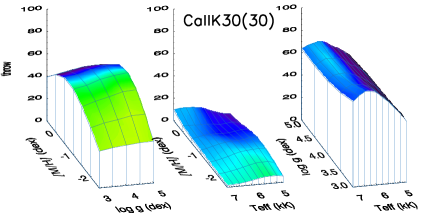
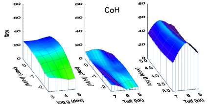
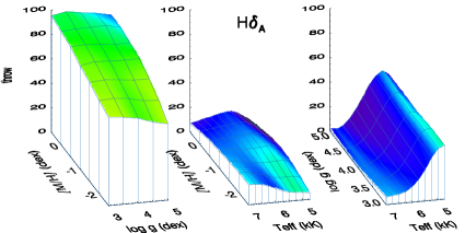
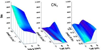
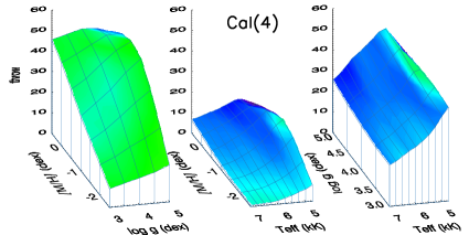
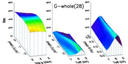
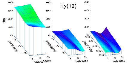
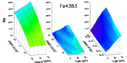
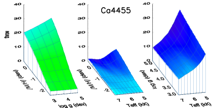
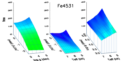
Figure 6: Throw vs. $T_{\rm eff}$ (left plot of each index), $\log{g}$ (middle plot), and [M/H] (right plot). Note that the temperature scale is increasing from right to left.

Figure 7: Spectroscopic indices as a function of interstellar extinction. The value of each index is compared to the respective value of the index without extinction.

Figure 8: Dependence of the indices to instrumental spectral resolution. The values of each index are compare to the respective value at 2.5 Å of resolution.

We also explored the dependence of the indices to extinction and instrumental spectral resolution, using as a reference the Munari’s synthetic spectrum (5750,4.5,0.0). The effect of reddening is obtained by applying the curve of Cardelli et al. (1989), increasing $A_{V}$ from 0 to 1 mag, and it is shown in Fig. 7. The only index that shows a variation of the same order of its typical error is G-whole(28), because its bands are defined over a wide wavelength interval (424 Å). In terms of the throw, this means that an error of 1 mag in $A_{V}$ estimation for a star introduces an error of $\pm$1.5 throws, which has to be compared with the values depicted in Fig. 6 to translate this uncertainty in terms of atmospheric parameters error. The effect of the extinction is much less for the other indices, being negligible for those defined in narrow wavelength intervals, such as CaI(4) or Ca4455.

Conversely, narrow band indices not affected by interstellar extinction might be subject to resolution effects. We have explored the effects of instrumental resolution by degrading the above model flux from 1.5 to 3.5 Å FWHM at a step of 0.1 Å (see Fig. 8). The most sensitive index is CaI(4), as its bandwidths are very narrow (4 Å). Similarly, the narrow side bands (5 Å width) are also the cause of the large variation shown by Ca II K30(30). However, the bandwidth is not the only quantity that matters, as the other index that show a change larger than its throw is CN₁, whose bands are at least 30 Å wide. In this case, the spectral morphology is also relevant since two strong feature dominated by Fe i are placed very near the limits of the central band. This property makes this index also prone to be sensitive to the precision of the wavelength calibration of observed spectra.

5 Determination of effective temperature, surface gravity, and metallicity.

Prior to the ultimate goal, we opted to extend the grid of synthetic indices. The parameter space coverage of Munari’s library is too coarse, with steps of 250 K in $T_{\rm eff}$, 0.5 dex in $\log{g}$ and 0.5 dex in [M/H]. We therefore performed a trilinear interpolation of the grid of calibrated indices to significantly reduce the steps to values that are smaller than the expected errors: 5 K in $T_{\rm eff}$, 0.05 dex in surface gravity and 0.02 dex in metallicity. This denser grid of indices includes more than 1.2 million entries.

We adopted a least squares method to determine the atmospheric parameters of the sample of target stars, by minimizing the statistic:

$$\rm{\chi^{2}}=\frac{1}{n}\displaystyle\sum^{n}_{i=1}\frac{\left(I_{i,teo}-I_{i,obs}\right)^{2}}{\sigma^{2}_{i,obs}}$$ (3)

where $I_{i,teo}$ and $I_{i,obs}$ are the theoretical and the observational indices, respectively, $n$ is the total number of indices, and $\sigma_{i,obs}$ is the error associated to each index of the observed spectrum. The combination of theoretical stellar parameters, whose indices provide the minimum $\chi^{2}$, was assigned to the corresponding star.

Figure 9: Residual spectrum in the Fe4531 interval of the star BD+60 600, after the first iteration of the procedure described in Sect. 5

A critical point in this procedure is a correct estimation of the errors $\sigma^{2}_{i,obs}$ in Eq. 3: since the blue interval of G-type stars is populated with thousands of non-negligible absorption lines, there is no wavelength interval, at a resolution of FWHM=2.5 Å, where the noise can be safely measured on the observed spectra. Therefore, we devised an iterative method that includes the following steps:

Table 5: Stellar atmospheric parameters. (The full version of the table is available in electronic form as Supporting Information in the online version of the article.)

Object	T${}_{\tiny\mbox{eff}}$ (K)	$\sigma_{\tiny\mbox{T}_{\mbox{eff}}}$ (K)		$\log g$ (dex)	$\sigma_{\tiny\mbox{log g}}$ (dex)		$\left[\mbox{M/H}\right]$ (dex)	$\sigma_{\tiny\mbox{[M/H]}}$ (dex)
		+	-		+	-		+	-
Vesta	5750	35	50	4.50	0.15	0.25	-0.02	0.04	0.04
Ceres	5750	25	55	4.50	0.10	0.25	-0.02	0.04	0.04
HD 236373	6010	15	25	4.50	0.05	0.15	-0.18	0.02	0.02
1RXS J003845.9+332534	5815	50	50	4.70	0.25	0.20	-0.26	0.06	0.06
[BHG88] 40 1943	5805	95	140	3.85	0.50	0.70	-0.30	0.14	0.16

Figure 10: Atmospheric parameters distributions of the sample of target stars. The shaded area shows the locations of the outliers (see text). The black area shows the SMR stellar sample. Fot the sake of clarity, in the right panel we do not include the “outlier” BD+34 4028, for which we determined [M/H]=$-$2.1.

1. for each $i$-th index, we computed the average value of a moving standard deviation, with a 5 Å-wide window, over the whole index wavelength interval (from the bluer to the redder limit) on the observed spectrum, and we assumed this value as the estimation of the noise level. Note that, during the first iteration, the noise is definitely overestimated, because the observed spectrum contains all the absorption lines, whose contribution is minimized by using a moving standard deviation, but not completely eliminated;

2. the computed noise level is assumed as the standard deviation of a Gaussian distribution which is used to randomly add noise to each wavelength point inside the index interval, and then the index is calculated. This step is repeated 1000 times for each index, and we end up with distributions of index values, whose standard deviations provides $\sigma^{2}_{i,obs}$, which are entered in Eq. 3 to estimate the stellar parameters;

3. these parameters are interpolated in the Munari’s library and the corresponding spectrum is subtracted to the observed one to obtain a residual spectrum. In the ideal case, this spectrum should contain only the observational noise, but, since the synthetic spectra do not perfectly match observations, we can still expect some trace of spectral features. This is well described in Fig 9, where we show the residual spectrum, after the first iteration, for the index Fe4531 of the star BD+60 600;

4. the process is repeated until two consecutive iterations produce the same set of atmospheric parameters.

We used the distribution of $\chi^{2}$ values to estimate the error on the parameters, following Avni (1976). This is, all the combinations of parameters that have $\chi^{2}<{\rm MIN}(\chi^{2})+3.5$ generate a volume in the parameters space, whose extreme values along the three dimensions give the (commonly asymmetric) 68% confidence level error. The results are reported in Table 5 where we list the set of stellar parameters and the corresponding error estimates.

6 Results and comparison with previous works

In Fig. 10 we show the distributions of the three atmospheric parameters for the 233 stars in our sample which in general appear compatible with those expected for G0–G3 stars on the main sequence. Note that the dispersion of the surface gravity distribution is quite large which, as previously pointed out, might be ascribed to the lower precision of the adopted method in determining this parameter. The average 1$\sigma$ error associated to $\log{g}$ is 0.26 dex, while it is 0.056 dex for [M/H] and 55 K for $T_{\rm eff}$. These figures are obtained once the outliers, indicated with a shaded area in Fig. 10, are removed. We have identified as outliers the 10 objects for which the best fit described in the previous section yields a surface gravity at the lower boundary of the synthetic grid ($\log{g}=3.0)$. Two of these outliers, TYC 4497-874-1 and BD+34 4028, have $T_{\rm eff}$ much larger than the bulk of the sample (7000 K and 6890 K, respectively), and in fact their spectra, depicted in Fig. 11, clearly indicates that they are F or late-A stars. Their $B-V$ colors are compatible with higher temperature objects: from SIMBAD these colors are 0.45 for TYC 4497-874-1 and 0.23 for BD+34 4028, which according to the color index-spectral calibration of Pecaut, Mamajek & Bubar (2012), and assuming no extinction, would correspond to stars of types F5–F6 and A7–A8, respectively. The spectral classification of these stars, in particular that of BD+34 4028, which dates back to the early sixties (Barbier, 1962), should be revisited.

Figure 11: Spectra of the two stars with the highest $T_{\rm eff}$.

It remains to be investigated the origin of the discrepancies for the rest of the deviant objects. Plausible explanations can be, among others, that we are actually dealing with binaries with composite spectra that cannot be separated at the working resolution, objects that are highly variable or that (some of) these objects are also wrongly classified. The answer is beyond the scope of this paper. For now, the parameters of the outliers should be considered as uncertain, in particular for the other 8 stars with $\log{g}=3.0$ dex: BD+31 3699, BD+42 384, BD+58 681, BD+60 2506, HD 105898, HD 149996, BD+45 2871 and TYC 3619-1400-1. The 10 “outliers” can be easily identified in the electronic version of Table 5 and are indicated with the symbol ”*” after the stellar identification.

Figure 12: Top panels: Comparison of the $T_{\rm eff}$ determined in this work and the determinations by Masana et al. (2006) (left), Bailer-Jones (2011) (middle) and Casagrande et al. (2011) (right). The solid line indicates the slope unity. In the middle panel, the filled and empty circles stand, respectively, for the results of the p and pq models of Bailer-Jones (2011). For the sake of clarity, we have incorporated in this panel a bar indicating the average value of the 90% confidence intervals reported in Bailer-Jones (2011). Bottom panels: Comparison of the $\log{g}$ (left) and [M/H] (right) reported in Casagrande et al. (2011) and those derived in this study.

6.1 Comparison with previous works

In addition to the test with the solar spectra, a natural exercise to verify the global validity of the set of parameters we have derived is to extend the comparison with other determinations from the literature: we selected three sources that contain several of our target stars.

In the top panels of Fig. 12, we illustrate the comparison of the $T_{\rm eff}$ for the 20 stars in common with Masana et al. (2006) (left panel), who determined this parameter from $V$ and 2MASS infrared photometry, with the study of Bailer-Jones (2011) (middle panel), who also provides $BVJHK$ photometric estimation of $T_{\rm eff}$ for the objects in common (34 with his p-model and 37 with his pq-model), and with the work of Casagrande et al. (2011) (right panel), which also includes 22 stars of our sample and obtains $T_{\rm eff}$ by means of the infrared flux method (Casagrande et al., 2006). By inspection of these figures, we can readily see that our resulting effective temperatures show, albeit some dispersion, an overall good agreement with Masana et al. (2006) and Casagrande et al. (2011), while are highly discrepant, of the order of 250 K lower, when compared with the p-model of Bailer-Jones (2011). The disagreement, cannot be explained by the fixed gravity and metallicity he used in his calculations. Bailer-Jones (2011) data are consistent with the temperature scale of Bailer-Jones et al. (1997) that indicates a temperature for a G2V star of 6015$\pm$49 K, which is more than 200 K higher than the accepted value for the Sun. Significant differences have been also found by Waite et al. (2011) for the star HIP 68328: these authors find a temperature lower by about 450 K than that of Bailer-Jones (2011), which somewhat agrees with the average difference with our results at low temperature. The comparison with the pq-model temperatures of Bailer-Jones (2011) shows a slightly smaller, but still systematic, offset.

For the comparison of $\log{g}$ and [M/H], we have used the stars in common with Casagrande et al. (2011). They derive [Fe/H] from a calibration of Strömgren colors and $\log{g}$ from the fundamental relation involving mass, $T_{\rm eff}$, and bolometric luminosity. The comparison is depicted in the lower panels of Fig. 12 for the 22 stars that have both parameters available. The agreement is, in general, good. We have already mentioned that our gravity determinations are prone to large uncertainties, which translate in a larger dispersion of our data. However, our average $\log{g}$ of 4.23 dex is consistent with the 4.27 dex value of Casagrande et al. (2011). Regarding metallicity, it appears that we somewhat underestimate it, as the average value of the global abundances for Casagrande et al. (2011) data and ours are, respectively, -0.02 and -0.10 dex. Nevertheless, Casagrande et al. (2011) state that their metallicity scale is 0.1 dex higher than the previous results they use for comparison.

6.2 SMR stars

According to the results presented in Sect. 5, we identify 22 SMR stars, of which 20 are new identifications, with a global metallicity in excess of $+$0.16 dex, the most metallic being TYC 2655-3677-1, with [M/H]=$+$0.28${}^{+0.04}_{-0.06}$. This sample represents about 10% of the observed targets and about the same proportion when compared with the set of stars whose average metallicity exceeds the above value in the PASTEL catalogue.

In Fig. 13, we depict the $V$ band distribution of the sample of SMR stars (shaded histogram) compared to the distribution of the 246 SMR stars present in the PASTEL catalogue. This latter sample was selected based upon these criteria: $5400<T_{\rm eff}<6400$ K, $4.0<\log{g}<5.0$ dex and [M/H]$\geq$ $+$0.16 dex. The number of SMR stars with $V>8$ is significantly increased, from 79 to 100, as a result of our study. The stellar parameters of SMR objects are given in Table 6.

Table 6: Atmospheric parameters of SMR stars.

Object	T${}_{\tiny\mbox{eff}}$ (K)	$\sigma_{\tiny\mbox{T}_{\mbox{eff}}}$ (K)		$\log g$ (dex)	$\sigma_{\tiny\mbox{log g}}$ (dex)		$\left[\mbox{M/H}\right]$ (dex)	$\sigma_{\tiny\mbox{[M/H]}}$ (dex)
		+	-		+	-		+	-
TYC 1759-462-1	6140	80	75	3.65	0.45	0.40	0.20	0.12	0.12
BD+60 402	5985	75	70	4.30	0.40	0.40	0.22	0.08	0.10
TYC 1230-576-1	5665	85	75	4.40	0.35	0.30	0.16	0.10	0.08
HD 232824	5900	50	85	4.15	0.25	0.45	0.16	0.06	0.10
HD 237200	6045	40	70	4.25	0.25	0.40	0.18	0.04	0.06
HD 135633	6095	65	70	4.25	0.35	0.45	0.22	0.06	0.06
BD+28 3198	5840	25	45	4.00	0.10	0.25	0.24	0.04	0.06
Cl* NGC 6779 CB 471	5790	70	65	3.80	0.35	0.35	0.20	0.10	0.10
TYC 2655-3677-1	6220	45	50	4.15	0.30	0.25	0.28	0.04	0.06
HD 228356	6055	55	20	4.00	0.30	0.10	0.16	0.06	0.04
BD+47 3218	6050	45	60	4.05	0.25	0.35	0.16	0.04	0.08
[M96a] SS Cyg star 14	6195	35	40	4.00	0.25	0.25	0.24	0.04	0.06
TYC 3973-1584-1	6000	35	55	4.45	0.20	0.30	0.20	0.04	0.06
BD+52 3145	6095	35	50	3.95	0.20	0.25	0.26	0.06	0.06
TYC 3986-3381-1	5855	55	60	4.15	0.25	0.25	0.26	0.08	0.06
TYC 3982-2812-1	5895	60	50	4.30	0.30	0.25	0.18	0.06	0.06
TYC 3618-1191-1	5940	60	60	4.40	0.35	0.30	0.24	0.08	0.08
TYC 3986-758-1	5845	55	65	4.05	0.30	0.35	0.16	0.06	0.08
BD+60 600	5655	35	60	3.95	0.10	0.30	0.20	0.06	0.08
HD 283538	6005	25	40	4.00	0.10	0.25	0.16	0.04	0.06
HD 137510	5875	70	20	4.00	0.35	0.05	0.16	0.08	0.04
HD 212809	5975	60	50	4.55	0.30	0.25	0.16	0.04	0.06

Figure 13: $V$ magnitude distribution of SMR stars of this work (shaded area) and from PASTEL catalogue.

7 Summary

The stellar parameters (T_eff, $\log g$, [M/H]) of a sample of 233 stars with spectral types between G0V-G3V were determined through the comparison of a set of spectroscopic indices and those calculated from a segment of Munari’s library of synthetic spectra. This work provides the first spectroscopic determination of the stellar parameters for almost 70$\%$ (213) of the stars in our sample. The results obtained are compatible with the expected values for the considered spectral types, and in general agreement with previous determinations. In particular the effective temperature of Casagrande et al. (2011) and Masana et al. (2006). We nevertheless find significant incosistencies with Bailer-Jones (2011), particularly at the lower temperature edge ($\sim$5600 K).

We identified a new sample of 20 SMR stars plus two that were already known. The comparisons presented in Sect. 6.1 and that conducted with the solar spectrum gives us confidence that the SMR stars found in this work indeed represent bona fide targets for future searches of giant exoplanets. Additionally, the present sample and its planned extensions in number of objects and in wavelength converage will complement, for instance, the data set of Adibekyan et al. (2011) and the fainter sample included in Lee et al. (2008) in the investigation of the chemical evolution of the Galaxy.

References

- Adibekyan et al. (2011) Adibekyan, V. Z., Santos, N. C., Sousa, S. G., & Israelian, G. 2011, A&A, 535, L11
- Adibekyan et al. (2012) Adibekyan, V. Z., Santos, N. C., Sousa, S. G., et al. 2012, A&A, 543, A89
- Alibert, Mordasini & Benz (2004) Alibert, Y., Mordasini, C., & Benz, W. 2004, A&A, 417, L25
- Avni (1976) Avni, Y. 1976, ApJ, 210, 642
- Bailer-Jones (2011) Bailer-Jones, C.A.L. 2011, MNRAS, 411, 435
- Bailer-Jones et al. (1997) Bailer-Jones, C.A.L., Irwin, M., Gilmore, G., & von Hippel, T. 1997, MNRAS, 292, 157
- Barbier (1962) Barbier, M. 1962, Publ. Obs. Haute-Provence, 6, 57
- Bertone et al. (2004) Bertone, E., Buzzoni, A., Chávez, M., & Rodríguez-Merino, L.H. 2004, AJ, 128, 829
- Bertone et al. (2008) Bertone, E., Buzzoni, A., Chávez, M., & Rodríguez-Merino, L.H. 2008, A&A, 485, 823
- Bonifacio et al. (2000) Bonifacio, P., Caffau, E., & Molaro, P. 2000, A&ASS, 145, 473
- Boss (1997) Boss, A. P. 1997, Science, 276, 1836
- Bruntt et al. (2003) Bruntt, H., Grundahl, F., Tingley, B., et al. 2003, A&A, 410, 323
- Buzzoni et al. (2001) Buzzoni, A., Chavez, M., Malagnini, M.L., & Morossi, C. 2001, PASP, 113, 1365
- Cardelli et al. (1989) Cardelli, J. A., Clayton, G. C., & Mathis, J. S. 1989, ApJ, 345, 245
- Carretero (2007) Carretero, C. 2007, Ph. D. Thesis, Instituto de Astrofísica de Canarias, Poblaciones Estelares de Galaxias de Tipo Temprano en Cúmulos: Restricciones a los Escenarios de Formación
- Casagrande et al. (2006) Casagrande, L., Portinari, L., & Flynn, C. 2006, MNRAS, 373, 13
- Casagrande et al. (2011) Casagrande, L., Schönrich, R., Asplund, M., et al. 2011, A&A, 530, A138
- Castelli & Kurucz (2003) Castelli, F., & Kurucz, R. L. 2003, Modelling of Stellar Atmospheres, IAU Symp., 210, 20P
- Coelho (2014) Coelho, P. R. T. 2014, MNRAS, 440, 1027
- Eggen (1964) Eggen, O. J. 1964, AJ, 69, 570
- Fischer & Valenti (2005) Fischer, D.A., & Valenti, J. 2005, ApJ, 622, 1102
- Gonzalez (1998) Gonzalez, G. 1998, A&A, 334, 221
- Harlan & Taylor (1970) Harlan, E. A., & Taylor, D. C. 1970, AJ, 75, 165
- Heiter et al. (2014) Heiter, U., Soubiran, C., Netopil, M., & Paunzen, E. 2014, A&A, 561, A93
- Kurucz (1993) Kurucz, R. 1993, SYNTHE Spectrum Synthesis Programs and Line Data. Kurucz CD-ROM No. 18. Cambridge, Mass.: Smithsonian Astrophysical Observatory, 1993., 18,
- Lee et al. (2008) Lee, Y.S., Beers, T.C., Sivarani, T., et al. 2008, AJ, 136, 2022
- Liu et al. (2008) Liu, G. Q., Deng, L., Chávez, M., et al. 2008, MNRAS, 390, 665
- Masana et al. (2006) Masana, E., Jordi, C., & Ribas, I. 2006, A&A, 450, 735
- Molenda-Żakowicz et al. (2013) Molenda-Żakowicz, J., Sousa, S. G., Frasca, A., et al. 2013, MNRAS, 434, 1422
- Munari et al. (2005) Munari, U., Sordo, R., Castelli, F., & Zwitter, T. 2005, A&A, 442, 1127
- Neves et al. (2009) Neves, V., Santos, N. C., Sousa, S. G., Correia, A. C. M., Israelian, G. 2009, A&A, 497, 563
- Pecaut, Mamajek & Bubar (2012) Pecaut, M., Mamajek, E., Bubar, E. J. 2012, ApJ, 746, 154.
- Porto de Mello et al. (2014) Porto de Mello, G. F., da Silva, R., da Silva, L., & de Nader, R. V. 2014, A&A, 563, A52
- Rich (1988) Rich, R.M. 1988, AJ, 95, 828
- Santos et al. (2001) Santos, N. C., Israelian, G., & Mayor, M. 2001, A&A, 373, 1019
- Santos (2008) Santos, N. C. 2008, in The Metal-Rich Universe, ed. G. Israelian & G. Meynet. Cambridge Univ. Press, Cambridge, p. 17
- Soubiran et al. (2010) Soubiran, C., Le Campion, J.-F., Cayrel de Strobel, G., & Caillo, A. 2010, A&A, 515, A111
- Spinrad & Taylor (1969) Spinrad, H., & Taylor, B.J. 1969, ApJ, 157, 1279
- Taylor (1996) Taylor, B. J. 1996, ApJS, 102, 105
- Trager et al. (1998) Trager, S.C., Worthey, G., Faber, S.M., Burstein, D., & Gonzalez, J.J. 1998, ApJS, 116, 1
- Waite et al. (2011) Waite, I. A., Marsden, S. C., Carter, B. D. et al., 2011, Publications of the Astronomical Society of Australia, 28, 323
- Worthey & Ottaviani (1997) Worthey, G., & Ottaviani, D.L. 1997, ApJS, 111, 377
- Worthey et al. (1994) Worthey, G., Faber, S. M., Gonzalez, J. J., & Burstein, D. 1994, ApJS, 94, 687