Convergence rate of Bayesian tensor estimator:
Optimal rate without restricted strong convexity

Abstract

In this paper, we investigate the statistical convergence rate of a Bayesian low-rank tensor estimator. Our problem setting is the regression problem where a tensor structure underlying the data is estimated. This problem setting occurs in many practical applications, such as collaborative filtering, multi-task learning, and spatio-temporal data analysis. The convergence rate is analyzed in terms of both in-sample and out-of-sample predictive accuracies. It is shown that a near optimal rate is achieved without any strong convexity of the observation. Moreover, we show that the method has adaptivity to the unknown rank of the true tensor, that is, the near optimal rate depending on the true rank is achieved even if it is not known a priori.

Keywords: Tensor estimation, Fast convergence rate, Bayes estimator, CP-rank, Tucker-rank

1 Introduction

Tensor modeling is a powerful tool for representing higher order relations between several data sources. The second order correlation has been a main tool in data analysis for a long time. However, because of an increase in the variety of data types, we frequently encounter a situation where higher order correlations are important for transferring information between more than two data sources. In this situation, a tensor structure is required. For example, a recommendation system with a three-mode table, such as user $\times$ movie $\times$ context, is regarded as comprising the tensor data analysis (Karatzoglou et al., 2010). The noteworthy success of tensor data analysis is based on the notion of the low rank property of a tensor, which is analogous to that of a matrix. The rank of a tensor is defined by a generalized version of the singular value decomposition for matrices. This enables us to decompose a tensor into a few factors and find higher order relations between several data sources.

A naive approach to computing tensor decomposition requires non-convex optimization (Kolda and Bader, 2009). Several authors have proposed convex relaxation methods to overcome the computational difficulty caused by non-convexity (Liu et al., 2009; Signoretto et al., 2010; Gandy et al., 2011; Tomioka et al., 2011; Tomioka and Suzuki, 2013). The main idea of convex relaxations is to unfold a tensor into a matrix, and apply trace norm regularization to the matrix thus obtained. This technique connects low rank tensor estimation to the well-investigated convex low rank matrix estimation. Thus, we can apply the techniques developed in low rank matrix estimation in terms of optimization and statistical theories. To address the theoretical aspects, the authors of Tomioka et al. (2011) gave the statistical convergence rate of a convex tensor estimator that utilizes the so-called overlapped Schatten 1-norm defined by the sum of the trace norms of all unfolded matricizations. In Mu et al. (2014), it was showed that the bound given by Tomioka et al. (2011) is tight, but can be improved by a modified technique called square deal. The authors of Tomioka and Suzuki (2013) proposed another approach called latent Schatten 1-norm regularization that is defined by the infimum convolution of trace norms of all unfolded matricizations, and analyzed its convergence rate. These theoretical studies revealed the qualitative dependence of learning rates on the rank and size of the underlying tensor. However, one problem of convex methods is that reducing the problem to a matrix one may lead to computational efficiency at the expense of statistical efficiency.

The main question addressed in this paper is whether we can obtain a computationally tractable method that possesses a better learning rate than existing methods. To answer this question, we consider a Bayesian learning method. Bayesian tensor learning methods have been studied extensively (Chu and Ghahramani, 2009; Xu et al., 2013; Xiong et al., 2010; Rai et al., 2014). Basically, they construct a generative model of the tensor decomposition and place a prior probability on the decomposed components. As in convex methods, Bayesian methods have also been polished to efficiently process large datasets. Their statistical performances have been supported numerically, but only a few theoretical analyses have been provided.

In this paper, we present the learning rate of a Bayes estimator for low-rank tensor regression problems. The problem occurs in many applications, such as collaborative filtering, multi-task learning, spatio-temporal data analysis. The prior probability we consider here is the most basic one, which places Gaussian priors on decomposed components and an exponentially decaying prior on the rank (see Xiong et al. (2010); Xu et al. (2013); Rai et al. (2014)). Roughly speaking, we obtain the (near) optimal convergence rate,

$$\|\hat{A}-A^{*}\|_{n}^{2}=O_{p}\left(\frac{d^{*}(\sum_{k=1}^{K}M_{k})\log(K\sqrt{n(\sum_{k}M_{k})^{K}}}{n}\right),$$

where $n$ is the sample size, $\hat{A}$ is the Bayes estimator, $A^{*}$ is the true tensor, $d^{*}$ is the CP-rank of the true tensor (its definition will be given in Section 2), and $(M_{1},\dots,M_{K})$ is the size. Moreover, our analysis has the following favorable properties.

• The near optimal rate is shown without assuming any strong convexity on the empirical $L_{2}$ norm.

• Rank adaptivity is shown, that is, the convergence rate is automatically adjusted to the rank of the true tensor as if we knew it a priori.

In particular, the first property significantly differentiates our approach from existing approaches. A variant of strong convexity, such as restricted strong convexity (Bickel et al., 2009; Negahban et al., 2012), is usually assumed in convex sparse learning in order to derive a fast rate. However, for the analysis of the predictive accuracy of a Bayes estimator, a near optimal rate can be shown without such conditions.

To the best of our knowledge, this is the first result that shows (near) optimality of a computationally tractable low-rank tensor estimator.

2 Problem Settings

In this section, the problem setting of this paper is shown. Suppose that there exists the true tensor $A^{*}\in\mathbb{R}^{M_{1}\times\dots\times M_{K}}$ of order $K$, and we observe $n$ samples $D_{n}=\{(Y_{i},X_{i})\}_{i=1}^{n}$ from the following linear model:

$$Y_{i}=\langle A^{*},X_{i}\rangle+\epsilon_{i}.$$

Here, $X_{i}$ is a tensor in $\mathbb{R}^{M_{1}\times\dots\times M_{K}}$ and the inner product $\langle\cdot,\cdot\rangle$ is defined by $\langle A,X\rangle=\sum_{j_{1},\dots,j_{K}=1}^{M_{1},\dots,M_{K}}A_{j_{1},\dots,j_{K}}X_{j_{1},\dots,j_{K}}$ between two tensors $A,X\in\mathbb{R}^{M_{1}\times\dots\times M_{K}}$. $\epsilon_{i}$ is i.i.d. noise from a normal distribution $N(0,\sigma^{2})$ with mean $0$ and variance $\sigma^{2}$.

Now, we assume the true tensor $A^{*}$ is “low-rank.” The notion of rank considered in this paper is CP-rank (Canonical Polyadic rank) (Hitchcock, 1927a, b). We say a tensor $A\in\mathbb{R}^{M_{1}\times\dots\times M_{K}}$ has CP-rank $d^{\prime}$ if there exist matrices $U^{(k)}\in\mathbb{R}^{d^{\prime}\times M_{k}}~{}(k=1,\dots,K)$ such that $A_{j_{1},\dots,j_{K}}=\sum_{r=1}^{d^{\prime}}U^{(1)}_{r,j_{1}}U^{(2)}_{r,j_{2}}\dots U^{(K)}_{r,j_{K}},$ and $d^{\prime}$ is the minimum number to yield this decomposition. This is called CP-decomposition. When $A$ satisfies this relation for ${\bm{U}}=(U^{(1)},U^{(2)},\dots,U^{(K)})$, we write

$$A=A_{\bm{U}}=[[U^{(1)},U^{(2)},\dots,U^{(K)}]]=:\left(\sum\nolimits_{r=1}^{d^{\prime}}U^{(1)}_{r,j_{1}}U^{(2)}_{r,j_{2}}\dots U^{(K)}_{r,j_{K}}\right)_{j_{1},\dots,j_{K}}.$$ (1)

We denote by $d^{*}$ the CP-rank of the true tensor $A^{*}$.

In this paper, we investigate the predictive accuracy of the linear model with the assumption that $A^{*}$ has low CP-rank. Because of the low CP-rank assumption, the learning problem becomes more structured than an ordinary linear regression problem on a vector. There are two types of predictive accuracy: in-sample one and out-of-sample. The in-sample predictive accuracy of an estimator $\hat{A}$ is defined by

$$\|\hat{A}-A^{*}\|_{n}^{2}:=\frac{1}{n}\sum_{i=1}^{n}\langle X_{i},\hat{A}-A^{*}\rangle^{2},$$ (2)

where $\{X_{i}\}_{i=1}^{n}$ is the observed input samples. The out-of-sample one is defined by

$$\|\hat{A}-A^{*}\|_{L_{2}(P(X))}^{2}:={\mathrm{E}}_{X\sim P(X)}[\langle X,\hat{A}-A^{*}\rangle^{2}],$$ (3)

where $P(X)$ is the distribution of $X$ that generates the observed samples $\{X_{i}\}_{i=1}^{n}$ and the expectation is taken over independent realization $X$ from the observed ones.

Example 1

Tensor completion under random sampling. Suppose that we have partial observations of a tensor. A tensor completion problem consists of denoising the observational noise and completing the unobserved elements. In this problem, $X_{i}$ is independently identically distributed from a set $\{e_{j_{1},\dots,j_{K}}\mid 1\leq j_{k}\leq M_{k}~{}(k=1,\dots,K)\},$ where $e_{j_{1},\dots,j_{K}}$ is an indicator vector that has 1 at its $(j_{1},\dots,j_{K})$-element and 0 elsewhere, and thus, $Y_{i}$ is an observation of one element of $A^{*}$ contaminated with noise $\epsilon_{i}$.

The out-of-sample accuracy measures how accurately we can recover the underlying tensor $A^{*}$ from the partial observation. If $X_{i}$ is uniformly distributed, $\|\hat{A}-A^{*}\|_{L_{2}(P(X))}^{2}=\frac{1}{M_{1}\dots M_{K}}\|\hat{A}-A^{*}\|_{2}^{2}$, where $\|\cdot\|_{2}$ is the $\ell_{2}$-norm obtained by summing the squares of all the elements. If $K=2$, this problem is reduced to the standard matrix completion problem. In that sense, our problem setting is a wide generalization of the low rank matrix completion problem.

Example 2

Multi-task learning. Suppose that several tasks are aligned across a 2-dimensional space. For each task $(s,t)\in\{1,\dots,M_{1}\}\times\{1,\dots,M_{2}\}$ (indexed by two numbers), there is a true weight vector $a^{*}_{(s,t)}\in\mathbb{R}^{M_{3}}$. The tensor $A^{*}$ is an array of the weight vectors $a^{*}_{(s,t)}$, that is, $A^{*}_{s,t,j}=a^{*}_{(s,t),j}$.

The input vector $X_{i}$ is a vector of predictor variables for one specific task, say $(s,t)$, and takes a form such that $X_{i,(s^{\prime},t^{\prime},:)}=\begin{cases}x_{i}^{(s,t)}\in\mathbb{R}^{M_{3}},&((s^{\prime},t^{\prime})=(s,t)),\\ \bm{0},&(\text{otherwise}).\end{cases}$

By assuming $A^{*}$ is low-rank in the sense of CP-rank, the problem becomes a multi-task feature learning with a two dimensional structure in the task space (Romera-Paredes et al., 2013).

As shown in the examples, the estimation problem of low-rank tensor $A^{*}$ is a natural extension of low-rank matrix estimation. However, it has a much richer structure than matrix estimation. Thus far, some convex regularized learning problems have been proposed analogously to spectrum regularization on a matrix, and their theoretical analysis has also been provided. However, no method have been proved to be statistically optimal. There is a huge gap between a matrix and higher order array. One reason for this gap is the computational complexity of the convex envelope of CP-rank. It is well known that the trace norm of a matrix is a convex envelope of the matrix rank on a set of matrices with a restricted operator norm (Srebro et al., 2005). However, as for CP-rank, it becomes NP-hard to compute its convex envelope if $K\geq 3$.

In this paper, we present a Bayes estimator instead of the convex regularized one. It will be shown that our Bayes estimator shows a near optimal convergence rate with a much weaker assumption, while the learning procedure is computationally tractable. The rate is much improved as compared to that of the existing estimators.

3 Bayesian tensor estimator

We now provide the prior distribution of the Bayes estimator that is investigated in this paper. On a decomposition of a rank $d^{\prime}$ tensor $A=[[U^{(1)},U^{(2)},\dots,U^{(K)}]]~{}(U^{(k)}\in\mathbb{R}^{d^{\prime}\times M_{k}})$, we place a Gaussian prior:

$$\pi(U^{(1)},\dots,U^{(K)}|d^{\prime}) \propto\exp\bigg{\{}-\frac{d^{\prime}}{2\sigma_{\mathrm{p}}^{2}}\sum_{k=1}^{K}\mathrm{Tr}[{U^{(k)}}^{\top}U^{(k)}]\bigg{\}},$$ (4)

where $\sigma_{\mathrm{p}}>0$. Moreover, we placed a prior distribution on the rank $1\leq d^{\prime}\leq d_{\max}$ as

$$\pi(d^{\prime})={\textstyle\frac{1}{N_{\xi}}}\xi^{d^{\prime}(M_{1}+\dots+M_{K})},$$

where $0<\xi<1$ is some positive real number, $d_{\max}$ is a sufficiently large number that is supposed to be larger than $d^{*}$, and $N_{\xi}$ is the normalizing constant, $N_{\xi}=\frac{1-\xi^{M_{1}+\dots+M_{K}}}{\xi-\xi^{d_{\max}(M_{1}+\dots+M_{K})}}$.

Now, since the noise is Gaussian, the likelihood of a tensor $A$ is given by

$$p(D_{n}|A)=:p_{n,A}\propto\exp\left\{-\frac{1}{2\sigma^{2}}\sum_{i=1}^{n}(Y_{i}-\langle A,X_{i}\rangle)^{2}\right\}.$$

The posterior distribution is given by

$$\Pi(A\in\mathcal{C}|D_{n})=\frac{\sum_{d=1}^{d_{\max}}\int_{A_{\bm{U}}\in\mathcal{C}}p_{n,A_{\bm{U}}}\pi(U^{(1)},\dots,U^{(K)}|d)\pi(d)\mathrm{d}U^{(1)}\dots\mathrm{d}U^{(K)}}{\sum_{d=1}^{d_{\max}}\int p_{n,A_{\bm{U}}}\pi(U^{(1)},\dots,U^{(K)}|d)\pi(d)\mathrm{d}U^{(1)}\dots\mathrm{d}U^{(K)}},$$

where $\mathcal{C}\subseteq\mathbb{R}^{M_{1}\times\dots M_{K}}$. It is noteworthy that the posterior distribution of $U^{(k)}$ conditioned by $d$ and $U^{(k^{\prime})}~{}(k^{\prime}\neq k)$ is a Gaussian distribution, because the prior is conjugate to Gaussian distributions. Therefore, the posterior mean $\int_{A}f(A)\Pi(\mathrm{d}A|D_{n})$ of a function $f:\mathbb{R}^{M_{1}\times\dots M_{K}}$ can be computed by an MCMC method, such as Gibbs sampling (Xiong et al., 2010; Xu et al., 2013; Rai et al., 2014). In this paper, we consider the posterior mean estimator $\hat{A}=\int A\Pi(\mathrm{d}A|D_{n})$ which is the Bayes estimator corresponding to the square loss.

4 Convergence rate analysis

In this section, we present the statistical convergence rate of the Bayes estimator. Before we give the convergence rate, we define some quantities and provide the assumptions. We define the max-norm of $A^{*}$ as

$$\|A^{*}\|_{\max,2}:=\min_{\{U^{(k)}\}}\{\max_{i,k}\|U^{(k)}_{:,i}\|_{2}\mid A^{*}=[[U^{(1)},\dots,U^{(K)}]],~{}U^{(k)}\in\mathbb{R}^{d^{*}\times M_{k}}\}.$$

The $\ell_{p}$-norm of a tensor $A$ is given by $\|A\|_{p}:=(\sum_{j_{1},\dots,j_{K}}|A_{j_{1},\dots,j_{K}}|^{p})^{\frac{1}{p}}$. The prior mass around the true tensor $A^{*}$ is a key quantity for characterizing the convergence rate, which is denoted by $\Xi$:

$$\Xi(\delta):=-\log(\Pi(A:\|A-A^{*}\|_{n}<\delta)),$$

where $\delta>0$. Small $\Xi(\delta)$ means that the prior is well concentrated around the truth. Thus, it is natural to consider that, if $\Xi$ is large, the Bayes estimator could be close to the truth. However, clearly, we do not know beforehand the location of the truth. Thus, it is not beneficial to place too much prior mass around one specific point. Instead, the prior mass should cover a wide range of possibilities of $A^{*}$. The balance between concentration and dispersion has a similar meaning to that of the bias-variance trade-off.

To normalize the scale, we assume that the $\ell_{1}$-norm of $X_{i}$ is bounded.

Assumption 1

We assume that the $\ell_{1}$-norm of $X_{i}$ is bounded by 1: $\|X_{i}\|_{1}\leq 1,~{}~{}\text{a.s.}.$

For theoretical simplicity, we utilize the unnormalized prior on the rank, that is $\pi(d)=\xi^{d(\sum_{k}M_{k})}$ . It should be noted that removing the normalization constant does not affect the posterior. Under these assumptions, $\Xi(\delta)$ can be bounded as follows.

Lemma 1

Under Assumption 1, the prior mass $\Xi$ has the bound

$$\Xi({\textstyle\frac{r}{\sqrt{n}}})\leq d^{*}\left(\sum_{k=1}^{K}M_{k}\right)\log\left[\frac{6}{\xi}\bigg{(}{\textstyle\frac{\sqrt{n}\sigma_{\mathrm{p}}^{K}K\left(\frac{\|A^{*}\|_{\max,2}}{\sigma_{\mathrm{p}}}+1\right)^{K-1}}{r}}\vee 1\bigg{)}\right]+\frac{d^{*}\sum_{k=1}^{K}\|U^{*(k)}\|_{F}^{2}}{2\sigma_{\mathrm{p}}^{2}}$$

for all $r>0$, where $\{U^{*(k)}\}_{k}$ are any tensors satisfying $A^{*}=[[U^{*(1)},\dots,U^{*(K)}]]$.

It should be noted that $\Xi(r/\sqrt{n})\leq\Xi(1/\sqrt{n})$ for all $r>1$. Finally, we define the technical quantities $C_{n,K}:=3K\sqrt{n}\left(\frac{4\sigma_{\mathrm{p}}^{2}\Xi(\frac{1}{\sqrt{n}})}{d^{*}}\right)^{\frac{K}{2}}$ and $c_{\xi}:=\min\{|\log(\xi)|/\log(C_{n,K}),1\}/4$.

4.1 In-sample predictive accuracy

We now give the convergence rate of the in-sample predictive accuracy. We suppose the inputs $\{X_{i}\}_{i=1}^{n}$ are fixed (not random). The in-sample predictive accuracy conditioned by $\{X_{i}\}_{i=1}^{n}$ is given as follows.

Theorem 1

Under Assumption 1, there exists a universal constant $C$ such that the posterior mean of the in-sample accuracy is upper bounded by

$${\mathrm{E}}\left[\int\|A-A^{*}\|_{n}^{2}\mathrm{d}\Pi(A|Y_{1:n})\right]\leq\frac{C}{n}\Bigg{[} d^{*}\left(\sum\nolimits_{k}M_{k}+\frac{1}{|\log(\xi)|}\right)\log(C_{n,K})+\frac{\Xi({\small\sqrt{\frac{c_{\xi}}{n}}})}{c_{\xi}}$$

$$+\log(d_{\max})+K+8^{K}(K+1)!\Bigg{]}.$$ (5)

The proof is given in Appendix A.2. This theorem provides the speed at which the posterior mass concentrates around the true $A^{*}$. It should be noted that the integral in the LHS of Eq. (5) is taken outside $\|A-A^{*}\|_{n}^{2}$. This gives not only information about the posterior concentration but also the convergence rate of the posterior mean estimator. This can be shown as follows. By Jensen’s inequality, we have ${\mathrm{E}}\left[\|\int A\mathrm{d}\Pi(A|Y_{1:n})-A^{*}\|_{n}^{2}\right]\leq{\mathrm{E}}\left[\int\|A-A^{*}\|_{n}^{2}\mathrm{d}\Pi(A|Y_{1:n})\right]$. Therefore, Theorem 1 gives a much stronger claim on the posterior than just stating the convergence rate of the posterior mean estimator.

Since the rate (5) is rather complicated, we give a simplified bound. By assuming $\log(d_{\max})$ and $K!$ are smaller than $d^{*}(\sum_{k}M_{k})$, we rearrange it as

$${\mathrm{E}}\left[\int\|A-A^{*}\|_{n}^{2}\mathrm{d}\Pi(A|Y_{1:n})\right]=O\left(\frac{d^{*}(M_{1}+\dots+M_{K})}{n}\log\bigg{(}K\sqrt{n({\textstyle\sum_{k=1}^{K}M_{k}})^{K}}\frac{\sigma_{\mathrm{p}}^{K}}{\xi}\bigg{)}\right).$$

Inside the $O(\cdot)$ symbol, a constant factor depending on $K,\|A^{*}\|_{\max,2},\sigma_{\mathrm{p}},\xi$ is hidden. This bound means that the convergence rate is characterized by the actual degree of freedom up to a log term. That is, since the true tensor has rank $d^{*}$ and thus has a decomposition (1), the number of unknown parameters is bounded by $d^{*}(M_{1}+\dots+M_{K})$. Thus, the rate is basically $O(\frac{\text{degree of freedom}}{n})$ (up to $\log$ order), which is optimal. Here, we would like to emphasize that the true rank $d^{*}$ is unknown, but by placing a prior distribution on a rank the Bayes estimator can appropriately estimate the rank and gives an almost optimal rate depending on the true rank. In this sense, the Bayes estimator has adaptivity to the true rank.

More importantly, we do not assume any strong convexity on the design. Usually, to derive a fast convergence rate of sparse estimators, such as Lasso and the trace norm regularization estimator, we assume a variant of strong convexity, such as a restricted eigenvalue condition (Bickel et al., 2009) and restricted strong convexity (Negahban et al., 2012). However, our convergence rate does not require such conditions. This is a quite strong point in our analysis. One reason why this is possible is that we are interested in the predictive accuracies rather than the actual distance between the tensors $\|A-A^{*}\|_{2}^{2}$. It is difficult to check the strong convexity condition in practice. However, we do not need to consider this when we are interested only in the predictive accuracy.

4.2 Out-of-sample predictive accuracy

Next, we turn to the convergence rate of the out-of-sample predictive accuracy. In this setting, the input sequence $\{X_{i}\}_{i=1}^{n}$ is not fixed, but an i.i.d. random variable generated by a distribution $P(X)$.

To obtain fast convergence of the out-of-sample accuracy, we need to bound the difference between the empirical and population $L_{2}$-errors: $\|A-A^{*}\|_{n}^{2}-\|A-A^{*}\|_{L_{2}(P(X))}^{2}$. To ensure that this quantity is small using Bernstein’s inequality, $\max_{X}|\langle X,A\rangle|$ should be bounded. However, the infinity norm of the posterior mean could be large in tensor estimation. This difficulty can be avoided by rejecting posterior sample $A$ with a large infinity norm.

4.2.1 Rejection sampling with infinity norm thresholding

Now, define $\|A\|_{\infty}=\max_{j_{1},\dots,j_{K}}|A_{j_{1},\dots,j_{K}}|$. Then, under Assumption 1, we have $\langle X,A\rangle\leq\|A\|_{\infty}$. Here, we assume that the infinity norm $\|A^{*}\|_{\infty}$ of the true tensor is approximately known, that is, we know $R>0$ such that $2\|A^{*}\|_{\infty}<R$. This is usually true. For example, we know the upper bound in tensor completion for a recommendation system. Otherwise, we may apply cross validation. Our strategy is to reject the posterior samples with an infinity norm larger than $R$ during the sampling scheme.

The resultant distribution of rejection sampling is the conditional posterior distribution $\Pi(\cdot|\|A\|_{\infty}\leq R,D_{n})$. Accordingly, we investigate the out-of-sample accuracy of the conditional posterior:

$${\mathrm{E}}_{D_{n}}\left[\int\|A-A^{*}\|_{L_{2}(P(X))}^{2}\mathrm{d}\Pi(A|\|A\|_{\infty}\leq R,D_{n})\right].$$

It should be noted that the conditional posterior is interpreted as the proper posterior distribution corresponding to the “truncated” prior the support of which is restricted to $\|A\|_{\infty}\leq R$.

Theorem 2

Suppose Assumption 1 and $\|A^{*}\|_{\infty}<\frac{1}{2}R$ are satisfied, then the out-of-sample accuracy is bounded as

$${\mathrm{E}}_{D_{n}}\left[\int\|A-A^{*}\|_{L_{2}(P(X))}^{2}\mathrm{d}\Pi(A|\|A\|_{\infty}\leq R,D_{n})\right]$$

$$\leq \frac{C(R^{2}\vee 1)}{n}\Bigg{[}d^{*}\left(\sum\nolimits_{k}M_{k}+\frac{3}{|\log(\xi)|}\right)\log(C_{n,K})+\frac{\Xi(\sqrt{\frac{c_{\xi}}{n}})}{c_{\xi}}+\log(d_{\max})+8^{K}(K+1)!\Bigg{]},$$

where $C$ is a universal constant.

The proof is given in Appendix B. The only difference between this and Theorem 1 is that $R^{2}$ appears in front of the bound. The source of this factor is the gap between the empirical and population $L_{2}$-norms. Here again, the convergence rate can be simplified as

$${\mathrm{E}}_{D_{n}}\left[\int\|A-A^{*}\|_{L_{2}(P(X))}^{2}\mathrm{d}\Pi(A|\|A\|_{\infty}\leq R,D_{n})\right]$$

$$\leq O\left(\frac{d^{*}(M_{1}+\dots+M_{K})}{n}(R^{2}\vee 1)\log\bigg{(}K\sqrt{n({\textstyle\sum_{k=1}^{K}M_{k}})^{K}}\frac{\sigma_{\mathrm{p}}^{K}}{\xi}\bigg{)}\right),$$ (6)

if $K!$ and $|\log(\xi)|$ are sufficiently smaller than $d^{*}(\sum_{k}M_{k})$. Here, we observe that the convergence rate achieved is optimal up to the $\log$-term. We would like to emphasize again that the optimal rate is achieved, although we do not assume any strong convexity on the distribution $L_{2}(\Pi)$. This can be so because we are not analyzing the actual $L_{2}$-norm $\|A-A^{*}\|_{2}$. If we do not assume strong convexity like $\|A-A^{*}\|_{2}\leq C\|A-A^{*}\|_{L_{2}(P(X))}$, it is impossible to derive fast convergence of $\|A-A^{*}\|_{2}$. The trick is that we focus on the “weighted” $L_{2}$-norm $\|A-A^{*}\|_{L_{2}(P(X))}$ instead of $\|A-A^{*}\|_{2}$.

Finally, it is remarked that, if $X_{i}$ is the uniform at random observation in the tensor completion problem, then $\|A-A^{*}\|_{L_{2}(P(X))}^{2}=\frac{1}{\prod_{k}M_{k}}\|A-A^{*}\|_{2}^{2}$ (note that in this setting $\|X_{i}\|_{1}=1$). Thus, our analysis yields fast convergence of the tensor recovery. If $K=2$, the analysis recovers the well known rate of matrix completion problems up to a $\log(nM_{1}M_{2})$ term (Negahban and Wainwright, 2012; Negahban et al., 2012; Rohde and Tsybakov, 2011):

$$\frac{1}{M_{1}M_{2}}\|\hat{A}-A^{*}\|_{2}^{2}=O_{p}\left(\frac{d^{*}(M_{1}+M_{2})}{n}\log(nM_{1}M_{2})\right).$$

4.2.2 Rejection sampling with max-norm thresholding

Finally, we briefly describe the convergence rate of the Bayes estimator based on the rejection sampling with respect to restricted max-norm. We reject the posterior sample with a max-norm larger than $R$; that is, we accept only a sample $A_{\bm{U}}$ that satisfies $\bm{U}\in\{(U^{(1)},\dots,U^{(K)})\mid\|U^{(k)}_{:,j}\|\leq R~{}(1\leq k\leq K,1\leq j\leq M_{k})\}=:\mathcal{U}_{R}$. Then, we have the following bound.

Theorem 3

Under Assumption 1 and $\|A^{*}\|_{\max,2}+\sigma_{\mathrm{p}}<R$, we have

$${\mathrm{E}}_{D_{n}}\left[\int\!\|A_{\bm{U}}-A^{*}\|_{L_{2}(P(X))}^{2}\mathrm{d}\Pi(A_{\bm{U}}|\bm{U}\in\mathcal{U}_{R},D_{n})\right]$$

$$\leq C\Bigg{(}\frac{d^{*}(\sum_{k=1}^{K}M_{k})}{n}(1\vee R^{2K})\log\left(K\sqrt{n}R^{\frac{K}{2}}\frac{\sigma_{\mathrm{p}}^{K}}{\xi}\right)\Bigg{)},$$

where $C$ is a constant depending on $K,\log(d_{\max}),\sigma_{\mathrm{p}}$.

The proof is given in Appendix C. In a setting where $M_{k}$ is much larger than $R$, this bound gives a much better rate than the previous ones, because the term inside $\log$ is improved from $\prod M_{k}^{\frac{1}{2}}$ to $R^{\frac{K}{2}}$. On the other hand, the rejection rate during the sampling would be increased.

5 Related works

In this section, we describe the existing works and clarify their relation to our work. Recently, theoretical analyses of convex regularized low-rank tensor estimators have been developed. The pioneering work (Tomioka et al., 2011) analyzed a method that utilizes unfolded matricization of a tensor. Let $M=\prod_{k=1}^{K}M_{k}$ (the number of whole elements). The authors used so-called overlapped Schatten 1-norm regularization $\sum_{k=1}^{K}\|A^{(k)}\|_{\mathrm{Tr}}$ where $\|\cdot\|_{\mathrm{Tr}}$ is the trace norm and $A^{(k)}\in\mathbb{R}^{M_{k}\times M/M_{k}}$ is the mode-$k$ unfolding of a tensor $A$ that is a matrix obtained by unfolding the tensor with the $k$-th index fixed. Their analysis assumes the true tensor $A^{*}$ has a low Tucker-rank (Tucker, 1966). Tucker-rank is a general notion of CP-rank. In this sense, their analysis is more general than ours. However, strong convexity of the empirical and population $L_{2}$-norm is assumed. Under this setting and $n=M$, the following bound is obtained:

$$\frac{1}{M}\|\hat{A}-A^{*}\|_{2}^{2}\leq C\frac{d^{*}}{n}{\textstyle\left(\frac{1}{K}\sum_{k=1}^{K}\sqrt{\frac{M}{M_{k}}}\right)^{2}}.$$ (7)

It can be seen that our bound $\frac{d^{*}(\sum_{k=1}^{K}M_{k})}{n}\log(nM)$ is smaller than this bound; in particular, if $M_{k}$ is large, the difference is significantly large. In Mu et al. (2014), it was shown that the bound (7) is tight and cannot be improved if the overlapped Schatten 1-norm is used. In Mu et al. (2014), a novel method called square deal was proposed and was shown to achieve the following rate. For $n=M$,

$$\frac{1}{M}\|\hat{A}-A^{*}\|_{2}^{2}\leq C\frac{d^{*}}{n}{\textstyle\left(\prod_{k\in I_{1}}M_{k}+\prod_{k\in I_{2}}M_{k}\right)},$$

where $I_{1}$ and $I_{2}$ are any disjoint decomposition of index set $\{1,\dots,K\}$. This improves the rate (7), but is still larger than the rate of the Bayes estimator, because the product of $M_{k}$ appears instead of the sum.

Another study on the regularization approach was presented in Tomioka and Suzuki (2013). The authors proposed using the latent Schatten 1-norm: $\inf_{\{A_{k}\}:A=\sum_{k=1}^{K}A_{k}}\sum_{k=1}^{K}\|A_{k}^{(k)}\|_{\mathrm{Tr}}$, where $A_{k}^{(k)}\in\mathbb{R}^{M_{k}\times M/M_{k}}$ is the mode-$k$ unfolding of the tensor $A_{k}$. A nice point of this method is that it automatically finds the minimum rank direction, that is, the mode-$k$ unfolding $A^{*(k)}$ with the minimum rank. It was shown that the rate is

$$\frac{1}{M}\|\hat{A}-A^{*}\|_{2}^{2}\leq C\frac{d^{*}\max_{k=1}^{K}\{M_{k}+M/M_{k}\}}{n}.$$

This rate is also larger than that of the Bayes estimator. We would like to remark that this rate is obtained for the low “Tucker-rank” situation, which is more general than our low CP-rank setting, and thus, it is not best suited to our situation. However, it is not apparent that the latent Schatten 1-norm achieves the same rate as that of the Bayes estimator in low CP-rank settings.

As for Bayesian counter part, a Bayesian low rank matrix estimator is analyzed in Alquier (2013). The prior in this study is similar to ours with $K=2$, but, instead of placing prior on the rank, the authors placed a Gamma prior on the variance of the Gaussian prior. They utilized the novel PAC-Bayes technique (McAllester, 1998; Catoni, 2004) to show

$$\|\hat{A}-A^{*}\|_{n}^{2}\leq C\frac{d^{*}(M_{1}+M_{2})\log(nM_{1}M_{2})}{n}.$$

This work has a similar flavor to ours in the sense that no strong convexity is required to obtain the convergence rate. However, there are several points in which it differs from ours: our analysis deals with general tensor estimation $(K\geq 3)$ and gives a bound also on the out-of-sample predictive accuracy by utilizing the rejection sampling scheme, and the posterior concentration is also given ($\int\|A-A^{*}\|_{n}^{2}\mathrm{d}\Pi(A|D_{n})$ instead of $\|\hat{A}-A^{*}\|_{n}^{2}$ where $\hat{A}$ is the posterior mean). By virtue of the analysis of the out-of-sample predictive accuracy, our analysis is applicable to tensor completion (and, of course, to matrix completion). As for the Bayesian tensor estimator, in Zhou et al. (2013) a Bayes estimator of probabilistic tensors was investigated. The model applies fully observed multinomial random variables and the rank is determined beforehand. Therefore, the setting is quite different from ours.

6 Numerical experiments

We now present numerical experiments to justify our theoretical results. The problem is the tensor completion problem where each observation is a random selection of one element of $A^{*}$ with observational noise $N(0,1)$ (see Example 1). The true tensor $A^{*}$ was randomly generated such that each element of $U^{(k)}~{}(k=1,\dots,K)$ was uniformly distributed on $[-1,1]$. $\sigma_{\mathrm{p}}$ was set at 5, and the true tensor was estimated by the posterior mean obtained by the rejection sampling scheme with $R=10$. The experiments were executed in five different settings, called settings 1 to 5: $\{(M_{1},\dots,M_{K}),d^{*}\}=\{(10,10,10),4\},\{(10,10,40),5\},\{(20,20,30),8\},\{(20,30,40),5\},\{(30,30,40),6\}$. For each setting, we repeated the experiments five times and computed the average of the in-sample predictive accuracy and out-of-sample accuracy over all five repetitions. The number of samples was chosen as $n=n_{\mathrm{s}}\prod_{k}M_{k}$, where $n_{\mathrm{s}}$ varied from 0.3 to 0.9.

In addition to the actual accuracy, we considered the “scaled” accuracy, which is defined by $\|\hat{A}-A^{*}\|_{n}^{2}\times\left(\frac{\prod_{k}M_{k}}{d^{*}(\sum_{k}M_{k})}\right);$ the scaled out-of-sample accuracy is also defined in the same manner. Figure 2 shows the in-sample accuracies and the scaled in-sample accuracies against the sample ratio $n_{\mathrm{s}}$. The same plot for the out-of-sample accuracy is shown in Figure 2. It can be seen that the curves of the scaled accuracies in all settings are satisfactorily overlapped. This means that our bound accurately describes the sample complexity of the Bayesian tensor estimator, because according to our bounds the scaled accuracies should behave as $1/n_{s}$ up to a constant factor (and a $\log$ term). The figures show that the scaling factor given by our theories is well matched to the actual predictive accuracy.

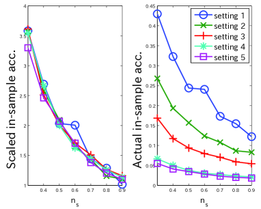
Figure 1: Scaled in-sample accuracy (left) and actual in-sample accuracy (right) versus $n_{s}$, averaged over five repetitions.

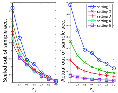
Figure 2: Scaled out-of-sample accuracy (left) and actual out-of-sample accuracy (right) versus $n_{s}$, averaged over five repetitions.

7 Conclusion and discussions

In this paper, we investigated the statistical convergence rate of a Bayesian low rank tensor estimator. The notion of a tensor’s rank in this paper was based on CP-rank. It is noteworthy that the predictive accuracy was bounded without any strong convexity assumption. Moreover, the obtained bound was (near) optimal and automatically adapted to the unknown rank. Numerical experiments showed that our theories indeed describe the actual behavior of the Bayes estimator.

Our bound includes the $\log$ term, which is not negligible when $K$ is large. However, numerical experiments showed that the scaling factor without the $\log$ term explains well the actual behavior. An investigation of whether the $\log$ term can be removed or not is an important future work.

A Proofs of Lemma 1 and Theorem 1

Let $M_{r,d}$ be a positive number that will be determined later on. Let $\mathcal{F}_{r,d}$ be

$$\mathcal{F}_{r,d}=\{A=[[U^{(1)},\dots,U^{(K)}]]\mid\max_{i,k}\|U_{:,i}^{(k)}\|_{2}\leq\sqrt{M_{r,d}},~{}U^{(k)}\in\mathbb{R}^{d\times M_{k}}\},$$

and $\mathcal{F}_{r}$ be $\cup_{d=1}^{M}\mathcal{F}_{r,d}$.

$$\|A^{*}\|_{\max,2}:=\min_{\{U^{(k)}\}}\{\max_{i,k}\|U^{(k)}_{:,i}\|\mid A^{*}=[[U^{(1)},\dots,U^{(K)}]],~{}U^{(k)}\in\mathbb{R}^{d\times M_{k}}\}.$$

$\sigma_{\mathrm{p},d^{*}}$ is denoted by $\sigma_{\mathrm{p}}/\sqrt{d^{*}}$.

A.1 Proof of Lemma 1

For $d^{*}$ dimensional vectors $u^{(k)}~{}(k=1,\dots,K)$, let

$$\langle u^{(1)},\dots,u^{(K)}\rangle:=\sum_{i=1}^{d^{\prime}}\prod_{k=1}^{K}u_{i}^{(k)}.$$

Then for $u^{(k)},~{}u^{*(k)}~{}(k=1,\dots,K)$, we have that

$$|\langle u^{(1)},\dots,u^{(K)}\rangle-\langle u^{*(1)},\dots,u^{*(K)}\rangle|$$

$$= |\sum_{k=1}^{K}\langle u^{*(1)},\dots,u^{*(k-1)},u^{(k)}-u^{*(k)},u^{(k+1)},\dots,u^{(K)}\rangle|$$

$$\leq \sum_{k=1}^{K}\|u^{*(1)}\|\cdots\|u^{*(k-1)}\|\|u^{(k)}-u^{*(k)}\|\|u^{(k+1)}\|\cdots\|u^{(K)}\|.$$ (8)

Therefore, if $\|u^{(k)}\|\leq\|A^{*}\|_{\max,2}+\sigma_{\mathrm{p}}$, $\|u^{(k)}-u^{*(k)}\|\leq\frac{\epsilon r}{K(\|A^{*}\|_{\max,2}+\sigma_{\mathrm{p}})^{K-1}}$ and $\|u^{*(k)}\|\leq\|A^{*}\|_{\max,2}$, then we have

$$|\langle u^{(1)},\dots,u^{(K)}\rangle-\langle u^{*(1)},\dots,u^{*(K)}\rangle|\leq\epsilon r.$$

Now, we consider two situations: (i) $\frac{\epsilon r}{K(\|A^{*}\|_{\max,2}+\sigma_{\mathrm{p}})^{K-1}}\leq\sqrt{d^{*}}\sigma_{\mathrm{p},d^{*}}$ and (ii) $\frac{\epsilon r}{K(\|A^{*}\|_{\max,2}+\sigma_{\mathrm{p}})^{K-1}}\geq\sqrt{d^{*}}\sigma_{\mathrm{p},d^{*}}$. (i) If $\frac{\epsilon r}{K(\|A^{*}\|_{\max,2}+\sigma_{\mathrm{p}})^{K-1}}\leq\sqrt{d^{*}}\sigma_{\mathrm{p},d^{*}}(=\sigma_{\mathrm{p}})$ and $\|u^{*(k)}\|\leq\|A^{*}\|_{\max,2}$, then $\|u^{(k)}\|\leq\|A^{*}\|_{\max,2}+\sigma_{\mathrm{p}}$. Hence, by Lemma 2, we have that

$$-\log(\Pi(A:\|A-A^{*}\|_{n}<\epsilon r|d^{*}))\leq-\log(\Pi(A:\|A-A^{*}\|_{\infty}<\epsilon r|d^{*}))$$

$$\leq -\sum_{i_{1},\dots,i_{K}}^{M_{1},\dots,M_{K}}\log\left(\Pi(U_{:,i_{k}}^{(k)}:\|U_{:,i_{k}}^{(k)}-U_{:,i_{k}}^{*(k)}\|\leq{\textstyle\frac{\epsilon r}{K(\|A^{*}\|_{\max,2}+\sigma_{\mathrm{p}})^{K-1}}})\right)$$

$$\leq \sum_{k=1}^{K}\sum_{i_{k}=1}^{M_{k}}\left\{-d^{*}\log\left[\frac{\epsilon r}{6\sigma_{\mathrm{p},d^{*}}\sqrt{d^{*}}K(\|A^{*}\|_{\max,2}+\sigma_{\mathrm{p}})^{K-1}}\right]+\frac{\|U_{:,i_{k}}^{*(k)}\|^{2}}{2\sigma_{\mathrm{p},d^{*}}^{2}}\right\}$$

$$\leq -d^{*}(\sum_{k=1}^{K}M_{k})\log\left[\frac{\epsilon r}{6\sigma_{\mathrm{p},d^{*}}\sqrt{d^{*}}K(\|A^{*}\|_{\max,2}+\sigma_{\mathrm{p}})^{K-1}}\right]+\frac{\sum_{k=1}^{K}\|U^{*(k)}\|_{F}^{2}}{2\sigma_{\mathrm{p},d^{*}}^{2}}.$$

(ii) On the other hand, if $\frac{\epsilon r}{K(\|A^{*}\|_{\max,2}+\sigma_{\mathrm{p}})^{K-1}}>\sigma_{\mathrm{p},d^{*}}\sqrt{d^{*}}$, we have that

$$-\log(\Pi(A:\|A-A^{*}\|_{n}<\epsilon r|d^{*}))\leq-d^{*}(\sum_{k=1}^{K}M_{k})\log\left(\frac{\sigma_{\mathrm{p},d^{*}}\sqrt{d^{*}}}{6\sigma_{\mathrm{p},d^{*}}\sqrt{d^{*}}}\right)+\frac{\sum_{k=1}^{K}\|U^{*(k)}\|_{F}^{2}}{2\sigma_{\mathrm{p},d^{*}}^{2}}.$$

Combining these inequality, we have that

$$-\log(\Pi(A:\|A-A^{*}\|_{n}<\epsilon r))\leq-\log(\Pi(A:\|A-A^{*}\|_{n}<\epsilon r|d^{*}))-\log(\pi(d^{*}))$$

$$\leq -d^{*}\left(\sum_{k=1}^{K}M_{k}\right)\log\left[\frac{1}{6}\left({\textstyle\frac{\epsilon r}{\sigma_{\mathrm{p}}K(\|A^{*}\|_{\max,2}+\sigma_{\mathrm{p}})^{K-1}}}\wedge 1\right)\right]+\frac{\sum_{k=1}^{K}\|U^{*(k)}\|_{F}^{2}}{2\sigma_{\mathrm{p},d^{*}}^{2}}-\log(\pi(d^{*}))$$

$$\leq d^{*}\left(\sum_{k=1}^{K}M_{k}\right)\log\left[\frac{6}{\xi}\left({\textstyle\frac{\sigma_{\mathrm{p}}^{K}K(\frac{\|A^{*}\|_{\max,2}}{\sigma_{\mathrm{p}}}+1)^{K-1}}{\epsilon r}}\vee 1\right)\right]+\frac{\sum_{k=1}^{K}\|U^{*(k)}\|_{F}^{2}}{2\sigma_{\mathrm{p},d^{*}}^{2}}.$$ (9)

The last line is by the definition of the unnormalized prior $\pi(d)=\xi^{d(\sum_{k}M_{k})}$. Later on we let $\epsilon=1/\sqrt{n}$. This gives Lemma 1.

A.2 Proof of Theorem 1

In this section, we fix $X_{1:n}$ and think it is not a random variable.

To prove the theorem, we utilize the technique developed by van der Vaart and van Zanten (2011). Their technique is originally developed to show the posterior convergence of Gaussian process regression and is based on theories by Ghosal et al. (2000) for the posterior convergence of non-parametric Bayes models. Although our situation is of parametric model, their technique is useful because ours is high dimensional singular model in which a standard asymptotic statistics for parametric models does not work.

For a set of tensors $\mathcal{F}_{r}$, an event $\mathcal{A}_{r}$ and a test $\phi_{r}$ (all of which are dependent on a positive real number $r>0$), it holds that, for $\epsilon>0$,

$${\mathrm{E}}\left[\int\|A-A^{*}\|_{n}^{2}\Pi(\mathrm{d}A|Y_{1:n})\right]$$

$$= {\mathrm{E}}\left[32\epsilon^{2}\int_{r>0}r\Pi(\|A-A^{*}\|_{n}\geq 4\epsilon r|Y_{1:n})\mathrm{d}r\right]$$

$$\leq 32\epsilon^{2}\int_{r>0}r^{K}\big{\{}{\mathrm{E}}\left[\phi_{r}\right]+P(\mathcal{A}_{r}^{c})$$

$$~{}~{}~{}~{}~{}~{}~{}~{}~{}~{}~{}~{}+{\mathrm{E}}[(1-\phi_{r})\bm{1}_{\mathcal{A}_{r}}\Pi(A\in\mathcal{F}_{r}^{c}|Y_{1:n})]$$

$$~{}~{}~{}~{}~{}~{}~{}~{}~{}~{}~{}~{}+{\mathrm{E}}[(1-\phi_{r})\bm{1}_{\mathcal{A}_{r}}\Pi(A\in\mathcal{F}_{r}:\|A-A^{*}\|_{n}^{2}\geq 4\epsilon r^{2K}|Y_{1:n})]\big{\}}\mathrm{d}r^{K}$$

$$=: 32\epsilon^{2}\int_{r>0}r^{K}(A_{r}+B_{r}+C_{r}+D_{r})\mathrm{d}r^{K}.$$ (10)

We give an upper bound of $A_{r}$, $B_{r}$, $C_{r}$ and $D_{r}$ in the following.

Step 1. The probability distribution of $Y_{1:n}$ with a true tensor $A$ (that means $Y_{i}=\langle X_{i},A\rangle+\epsilon_{i}$) is denoted by $P_{n,A}$. The expectation of a function $f$ with respect to $P_{n,A}$ is denoted by $P_{n,A}(f)$.

For arbitrary $r^{\prime}>0$, define $C_{j,r^{\prime},d}=\{A\in\mathcal{F}_{r,d}\mid jr^{\prime}\leq\sqrt{n}\|A-A^{*}\|_{n}\leq(j+1)r^{\prime}\}$. We construct a maximum cardinality set $\Theta_{j,r^{\prime},d}\subset C_{j,r^{\prime},d}$ such that each $A,A^{\prime}\in\Theta_{j,r^{\prime},d}$ satisfies $\sqrt{n}\|A-A^{\prime}\|_{n}\geq jr^{\prime}/2$. The cardinality of $\Theta_{j,r^{\prime},d}$ is equal to $D(jr^{\prime}/2,C_{j,r^{\prime},d},\sqrt{n}\|\cdot\|_{n})$ . Then, one can construct a test $\phi_{j,d}$ such that

$$P_{n,A^{*}}\phi_{j,d}\leq D(jr^{\prime}/2,C_{j,r,d},\sqrt{n}\|\cdot\|_{n})e^{-\frac{1}{2}(\frac{jr^{\prime}}{2}+q)^{2}}\leq D(jr^{\prime}/2,C_{j,r,d},\sqrt{n}\|\cdot\|_{n})e^{-\frac{1}{8}j^{2}r^{\prime 2}-\frac{1}{2}q^{2}},$$

$$\sup_{A\in C_{j,r^{\prime},d}}P_{n,A}(1-\phi_{j,d})\leq e^{-\frac{1}{2}\max(\frac{jr^{\prime}}{2}-q,0)^{2}}\leq e^{-\frac{j^{2}r^{\prime 2}}{16}+\frac{q^{2}}{2}},$$

for any $q>0$ (see van der Vaart and van Zanten (2011) for the details ). For each $d$, we construct a test $\phi_{d}$ as $\phi_{d}=\max_{j}\phi_{j,d}$. Then we have

$$P_{n,A^{*}}\phi_{d} \leq\sum_{j\geq 1}D(jr^{\prime}/2,C_{j,r^{\prime},d},\sqrt{n}\|\cdot\|_{n})e^{-\frac{1}{8}j^{2}r^{\prime 2}-\frac{1}{2}q^{2}}\leq\sum_{j\geq 1}D(r^{\prime}/2,\mathcal{F}_{r,d},\sqrt{n}\|\cdot\|_{n})e^{-\frac{1}{8}j^{2}r^{\prime 2}-\frac{1}{2}q^{2}}$$

$$\leq 9D(r^{\prime}/2,\mathcal{F}_{r,d},\sqrt{n}\|\cdot\|_{n})e^{-\frac{1}{8}r^{\prime 2}-\frac{1}{2}q^{2}}.$$

Here, by setting $\frac{1}{2}q^{2}=\log(D(r^{\prime}/2,\mathcal{F}_{r,d},\sqrt{n}\|\cdot\|_{n}))$, we have

$$P_{n,A^{*}}\phi_{d} \leq 9e^{-\frac{1}{8}r^{\prime 2}},$$

$$\sup_{A\in\mathcal{F}_{r,d}}P_{n,A}(1-\phi_{d}) \leq e^{-\frac{1}{16}j^{2}r^{\prime 2}+\log(D(r^{\prime}/2,\mathcal{F}_{r,d},\sqrt{n}\|\cdot\|_{n}))}.$$

Finally, we construct a test $\phi$ as the maximum of $\phi_{d}$, that is, $\phi=\max_{d\geq 1}\phi_{d}$. Then, we have

$$P_{n,A^{*}}\phi \leq 9e^{-\frac{1}{8}r^{\prime 2}+\log(d_{\max})}$$

$$\sup_{A\in\mathcal{F}_{r,d}}P_{n,A}(1-\phi) \leq e^{-\frac{1}{16}r^{\prime 2}+\log(D(r^{\prime}/2,\mathcal{F}_{r,d},\sqrt{n}\|\cdot\|_{n}))},$$

for all $d\geq 1$.

Substituting $4\sqrt{n}\epsilon r^{K}$ into $r^{\prime}$, we obtain

$$P_{n,A^{*}}\phi \leq 9e^{-2n\epsilon^{2}r^{2K}+\log(d_{\max})}$$ (11)

$$\sup_{A\in\mathcal{F}_{r,d}}P_{n,A}(1-\phi) \leq e^{-n\epsilon^{2}r^{2K}+\log(D(r^{\prime}/2,\mathcal{F}_{r,d},\sqrt{n}\|\cdot\|_{n}))}.$$ (12)

We define

$$A_{r}=P_{n,A^{*}}\phi.$$

From now on, we denote by $\phi_{r}$ the test constructed above to indicate that the test is associated to a specific $r$.

Step 2.

By Lemma 14 of van der Vaart and van Zanten (2011) and its proof, one can show that, for any $r>0$,

$$P\left[\int\frac{p_{n,A}}{p_{n,A^{*}}}\mathrm{d}\Pi(A)\geq e^{-\frac{n\epsilon^{2}r^{2}}{2}-\sqrt{n}\epsilon rx}\Pi(A:\|A-A^{*}\|_{n}<\epsilon r)\right]\leq e^{-\frac{x^{2}}{2}}.$$

Therefore, there exists an even $\mathcal{A}_{1,r}$ such that

$$P_{A^{*}}(\mathcal{A}_{1,r}^{c})\leq e^{-n\epsilon^{2}r^{2}/8},$$

and, on the event $\mathcal{A}_{1,r}$, it holds that

$$\int\frac{p_{n,A}}{p_{n,A^{*}}}\mathrm{d}\Pi(A)\geq e^{-n\epsilon^{2}r^{2}}\Pi(A:\|A-A^{*}\|_{n}<\epsilon r).$$

Moreover, it can be checked in a similar way that there exists an event $\mathcal{A}_{2,r}$ such that, for a some fixed constant $c_{\xi}<\frac{1}{2}$ (which will be determined later),

$$P_{A^{*}}(\mathcal{A}_{2,r}^{c})\leq\exp\left\{-\frac{1}{2}\left(\frac{\sqrt{c_{\xi}}\sqrt{n}\epsilon r^{K}}{2}+\frac{\log(\Pi(A:\|A-A^{*}\|_{n}<\sqrt{c_{\xi}}\epsilon r^{K}))}{\sqrt{c_{\xi}}\sqrt{n}\epsilon r^{K}}\vee 0\right)^{2}\right\},$$ (13)

and, on the event $\mathcal{A}_{2,r}$, it holds that

$$\int\frac{p_{n,A}}{p_{n,A^{*}}}\mathrm{d}\Pi(A)\geq e^{-c_{\xi}n\epsilon^{2}r^{2K}}.$$

Here, we note that, by a simple calculation, the RHS of Eq. (13) is bounded by

$$e^{-\frac{1}{16}c_{\xi}n\epsilon^{2}r^{2K}},$$

if $c_{\xi}n\epsilon^{2}r^{2K}\geq-8\log(\Pi(A:\|A-A^{*}\|_{n}<\sqrt{c_{\xi}}\epsilon r^{K}))$.

Now, define $\mathcal{A}_{r}=\mathcal{A}_{1,r}\cap\mathcal{A}_{2,r}$, then we have

$$B_{r}=P_{A^{*}}(\mathcal{A}_{r}^{c})\leq e^{-n\epsilon^{2}r^{2}/8}+\exp\left\{-\frac{1}{2}\left(\frac{\sqrt{c_{\xi}}\sqrt{n}\epsilon r^{K}}{2}+\frac{\log(\Pi(A:\|A-A^{*}\|_{n}<\sqrt{c_{\xi}}\epsilon r^{K}))}{\sqrt{c_{\xi}}\sqrt{n}\epsilon r^{K}}\vee 0\right)^{2}\right\}.$$

Step 3.

Since

$$\{\{U^{(k)}\}_{k=1}^{K}\in\mathbb{R}^{d\times M_{1}}\times\dots\times\mathbb{R}^{d\times M_{K}}\mid\max_{k,i}\|U_{:,i}^{(k)}\|_{2}\geq\sqrt{M_{r,d}}\}$$

$$\subseteq \{\{U^{(k)}\}_{k=1}^{K}\in\mathbb{R}^{d\times M_{1}}\times\dots\times\mathbb{R}^{d\times M_{K}}\mid\sum_{k=1}^{K}\|U^{(k)}\|_{2}^{2}\geq M_{r,d}\},$$

Proposition 1 yields the bound of the prior probability of $\mathcal{F}_{r}^{c}$ as

$$\Pi(\mathcal{F}_{r}^{c})=\sum_{d=1}^{M}\Pi(\mathcal{F}_{r,d}^{c})\pi(d)\leq\sum_{d=1}^{M}\exp\left[\frac{d\sum_{k}M_{k}}{2}+\frac{d\sum_{k}M_{k}}{2}\log\left(\frac{M_{r,d}}{d\sum_{k}M_{k}\sigma_{\mathrm{p},d}^{2}}\right)-\frac{M_{r,d}}{2\sigma_{\mathrm{p},d}^{2}}\right]\pi(d).$$

Therefore, its posterior probability in the event $\mathcal{A}_{r}$ is bounded as

$$C_{r} =P_{n,A^{*}}[\Pi(\mathcal{F}_{r}^{c}|Y_{1:n})\bm{1}_{\mathcal{A}_{r}}(1-\phi_{r})]$$

$$\leq\sum_{d=1}^{M}\exp\left[n\epsilon^{2}r^{2}+\Xi(\epsilon r)+\frac{d\sum_{k}M_{k}}{2}+\frac{d\sum_{k}M_{k}}{2}\log\left(\frac{M_{r,d}}{d\sum_{k}M_{k}\sigma_{\mathrm{p},d}^{2}}\right)-\frac{M_{r,d}}{2\sigma_{\mathrm{p},d}^{2}}\right]\pi(d).$$

Step 4.

Here, $D_{r}$ is evaluated. Remind that $D_{r}$ is defined as

$$D_{r}=P_{n,A^{*}}[\Pi(A\in\mathcal{F}_{r}:\|A-A^{*}\|_{n}>4\epsilon r^{K}|Y_{1:n})(1-\phi_{r})\bm{1}_{\mathcal{A}_{r}}].$$

Since $\mathcal{A}_{r}=\mathcal{A}_{1,r}\cup\mathcal{A}_{2,r}\supseteq\mathcal{A}_{2,r}$, we have

$$D_{r} \leq P_{n,A^{*}}\left[\sum_{d}\int_{A\in\mathcal{F}_{r,d}:\|A-A^{*}\|_{n}>4\epsilon r^{K}}p_{n,A}/p_{n,A^{*}}\mathrm{d}\Pi(A|d)\exp(c_{\xi}n\epsilon^{2}r^{2K})\pi(d)(1-\phi_{r})\bm{1}_{\mathcal{A}_{r}}\right]$$

$$=\sum_{d}\int_{A\in\mathcal{F}_{r,d}:\|A-A^{*}\|_{n}>4\epsilon r^{K}}P_{n,A}[(1-\phi_{r})\bm{1}_{\mathcal{A}_{r}}]\exp(c_{\xi}n\epsilon^{2}r^{2K})\mathrm{d}\Pi(A|d)\pi(d).$$

Therefore, using $P_{n,A}[(1-\phi_{r})\bm{1}_{\mathcal{A}_{r}}]\leq 1$, the summand in the RHS is bounded by

$$\pi(d)\exp(c_{\xi}n\epsilon^{2}r^{2K}).$$ (14)

Simultaneously, Eq. (12) gives another upper bound of the summand as

$$\int_{A\in\mathcal{F}_{r,d}:\|A-A^{*}\|_{n}>4\epsilon r^{K}}e^{c_{\xi}n\epsilon^{2}r^{2K}-n\epsilon^{2}r^{2K}+\log(D(2\sqrt{n}\epsilon r^{K},\mathcal{F}_{r,d},\sqrt{n}\|\cdot\|_{n})}\mathrm{d}\Pi(A|d)\pi(d)$$

$$\leq \pi(d)\exp\left\{-\frac{1}{2}n\epsilon^{2}r^{2K}+\log(D(2\sqrt{n}\epsilon r^{K},\mathcal{F}_{r,d}),\sqrt{n}\|\cdot\|_{n}))\right\},$$ (15)

for $r\geq 1$, where we used $c_{\xi}<\frac{1}{2}$.

We evaluate the packing number $\log(D(2\sqrt{n}\epsilon r^{K},\mathcal{F}_{r,d},\sqrt{n}\|\cdot\|_{n}))$. It is known that the packing number of unit ball in $d$-dimensional Euclidean space is bounded by

$$D(\epsilon,B_{d}(1),\|\cdot\|)\leq\left(\frac{4+\epsilon}{\epsilon}\right)^{d}.$$

Here $B_{d}(R)$ denotes the ball with the radius $R$ in $d$-dimensional Euclidean space.

Similar to Eq. (8), the $L_{2}$-norm between two tensors $A=[[U^{(1)},\dots,U^{(K)}]]$ and $A^{\prime}=[[U^{\prime(1)},\dots,U^{\prime(K)}]]$ can be bounded by

$$\|A-A^{\prime}\|_{2}^{2}= \sum_{i_{1},i_{2},\dots,i_{K}}(\langle U_{:,i_{1}}^{(1)},\dots,U_{:,i_{K}}^{(K)}\rangle-\langle U_{:,i_{1}}^{\prime(1)},\dots,U_{:,i_{K}}^{\prime(K)}\rangle)^{2}$$

$$= \sum_{i_{1},i_{2},\dots,i_{K}}\left(\sum_{k=1}^{K}\langle U_{:,i_{1}}^{(1)},\dots,U_{:,i_{k-1}}^{(k-1)},U_{:,i_{k}}^{(k)}-U_{:,i_{k}}^{\prime(k)},\dots,U_{:,i_{K}}^{\prime(K)}\rangle\right)^{2}$$

$$\leq K\sum_{i_{1},i_{2},\dots,i_{K}}\sum_{k=1}^{K}\langle U_{:,i_{1}}^{(1)},\dots,U_{:,i_{k-1}}^{(k-1)},U_{:,i_{k}}^{(k)}-U_{:,i_{k}}^{\prime(k)},U_{:,i_{k+1}}^{\prime(k+1)},\dots,U_{:,i_{K}}^{\prime(K)}\rangle^{2}$$

$$\leq K\sum_{k=1}^{K}\sum_{i_{1},i_{2},\dots,i_{K}}\|U_{:,i_{1}}^{(1)}\|_{2}^{2}\times\cdots\times\|U_{:,i_{k-1}}^{(k-1)}\|_{2}^{2}\times\|U_{:,i_{k}}^{(k)}-U_{:,i_{k}}^{\prime(k)}\|_{2}^{2}\times\|U_{:,i_{k+1}}^{\prime(k+1)}\|_{2}^{2}\times\cdots\times\|U_{:,i_{K}}^{\prime(K)}\|_{2}^{2}$$

$$\leq K\sum_{k=1}^{K}\|U^{(1)}\|_{2}^{2}\times\cdots\times\|U^{(k-1)}\|_{2}^{2}\|U^{(k)}-U^{\prime(k)}\|_{2}^{2}\times\|U^{\prime(k+1)}\|_{2}^{2}\times\cdots\times\|U^{\prime(K)}\|_{2}^{2}.$$

If $A,A^{\prime}\in\mathcal{F}_{r,d}$, then the RHS is further bounded by

$$\|A-A^{\prime}\|_{2}^{2}\leq KM_{r,d}^{K-1}\sum_{k=1}^{K}\|U^{(k)}-U^{\prime(k)}\|_{2}^{2}.$$ (16)

Thus, if $2\epsilon r^{K}\leq KM_{r,d}^{K/2}$, using the relation (16) and $\sqrt{n}\|A-A^{\prime}\|_{n}\leq\sqrt{n}\|A-A^{\prime}\|_{\infty}\leq\sqrt{n}\|A-A^{\prime}\|_{2}$, we have that

$$\log(D(2\sqrt{n}\epsilon r^{K},\mathcal{F}_{r,d},\sqrt{n}\|\cdot\|_{n}))\leq\log(D(2\epsilon r^{K},\mathcal{F}_{r,d},\|\cdot\|_{2}))$$

$$\leq\log(D(2\epsilon r^{K}/(KM_{r,d}^{(K-1)/2}),B_{d\sum_{k}M_{k}}(\sqrt{M_{r,d}}),\|\cdot\|_{2}))$$

$$\leq d\left(\sum_{k=1}^{K}M_{k}\right)\log\left(\frac{4+\frac{2\epsilon r^{K}}{KM_{r,d}^{K/2}}}{\frac{2\epsilon r^{K}}{KM_{r,d}^{K/2}}}\right)\leq d(\sum_{k=1}^{K}M_{k})\log\left(\frac{3KM_{r,d}^{K/2}}{\epsilon r^{K}}\right),$$ (17)

otherwise, $\log(D(2\sqrt{n}\epsilon r^{K},\mathcal{F}_{r,d}))=0$.

Combining Eqs. (14) and (15) with Eq. (17) results in the following upper bound of $D_{r}$:

$$D_{r}\leq\sum_{d}\pi(d)\min\left\{\exp(c_{\xi}n\epsilon^{2}r^{2K}),\exp\left[-\frac{1}{2}n\epsilon^{2}r^{2K}+d\left(\sum_{k=1}^{K}M_{k}\right)\log\left(\frac{3KM_{r,d}^{K/2}}{\epsilon r^{K}}\right)\right]\right\}$$ (18)

for $r\geq 1$.

Step 5.

Here, we establish the assertion by combining the bounds of $A_{r},~{}B_{r},~{}C_{r}$ and $D_{r}$ obtained above. Set $\epsilon=\frac{1}{\sqrt{n}}$ and $M_{r,d}=\frac{4}{\min(d^{*},d)}\Xi(1/\sqrt{n})\sigma_{\mathrm{p}}^{2}r^{2}$. Then, we have that, for all $d\geq d^{*}$,

$$d\left(\sum_{k=1}^{K}M_{k}\right)\log\left(\frac{3KM_{r,d}^{K/2}}{\epsilon r^{K}}\right)\leq d\left(\sum_{k=1}^{K}M_{k}\right)\log\left(3K\sqrt{n}\left(\frac{4\sigma_{\mathrm{p}}^{2}\Xi(\frac{1}{\sqrt{n}})}{d^{*}}\right)^{\frac{K}{2}}\right).$$

Recall that $C_{n,K}=3K\sqrt{n}\left(\frac{4\sigma_{\mathrm{p}}^{2}\Xi(\frac{1}{\sqrt{n}})}{d^{*}}\right)^{\frac{K}{2}}$, and $c_{\xi}=\min\{|\log(\xi)|/\log(C_{n,K}),1\}/4$. Let $\tilde{r}_{d}$ be such that $-\frac{1}{2}\tilde{r}_{d}^{2K}+d\left(\sum_{k=1}^{K}M_{k}\right)\log(C_{n,K})=0$, that is, $\tilde{r}_{d}=2^{1/2K}[d(\sum_{k}M_{k})\log(C_{n,K})]^{1/2K}$.

By the upper bound (10), we have that

$${\mathrm{E}}\left[\int\|A-A^{*}\|_{n}^{2}\mathrm{d}\Pi(A|Y_{1:n})\right]\leq 32\epsilon^{2}+32\epsilon^{2}\int_{r>1}r^{K}(A_{r}+B_{r}+C_{r}+D_{r})\mathrm{d}r^{K}.$$

We are going to bound each term in the integral.

$$\int_{r>1}r^{K}A_{r}\mathrm{d}r^{K}\leq\int_{r>1}r^{K}\min\{9\exp(-2r^{2K}+\log(d_{\max})),1\}\mathrm{d}r^{K}\leq\frac{\log(d_{\max})}{2}+\frac{9}{4}.$$

By Lemma 3, the integral related to $B_{r}$ is bounded by

$$\int_{r>1}r^{K}B_{r}\mathrm{d}r^{K} \leq 8\Xi(\sqrt{c_{\xi}}\epsilon)/c_{\xi}+\int_{r^{K}>\sqrt{8\Xi(\sqrt{c_{\xi}}\epsilon)/c_{\xi}}}r^{K}\left[\exp(-r^{2}/8)+\exp(-c_{\xi}r^{2K}/16)\right]\mathrm{d}r^{K}$$

$$\leq 8\frac{\Xi(\sqrt{c_{\xi}}\epsilon)}{c_{\xi}}+\int_{r^{K}>1}r^{K}\exp(-r^{2}/8)\mathrm{d}r^{K}$$

$$~{}~{}~{}~{}+\frac{1}{32}\exp\left(-\frac{\Xi(\sqrt{c_{\xi}}\epsilon)}{2c_{\xi}}\right).$$

Here, the second term of the RHS is bounded by

$$\int_{r^{K}>1}r^{K}\exp(-r^{2}/8)\mathrm{d}r^{K}\leq\frac{1}{2}\sum_{j=1}^{K}8^{j}\frac{K!}{(K-j)!}\exp\left(-\frac{1}{8}\right)\leq 8^{K}(K+1)!.$$

Similarly, by Lemma 3, the integral related to $C_{r}$ is bounded by

$$\int_{r>1}r^{K}C_{r}\mathrm{d}r^{K} \leq\int_{r>1}r^{K}\sum_{d=1}^{M}\exp\left[-\frac{d}{\min(d,d^{*})}\Xi(\epsilon)r^{2}\right]\pi(d)\mathrm{d}r^{K}$$

$$\leq\frac{1}{2}\sum_{j=0}^{K-1}\frac{K\cdots(K-j)}{\Xi(1/\sqrt{n})^{j+1}}\leq K.$$

Next, we bound the integral corresponding to $D_{r}$. By the definition of $c_{\xi}$ and $\tilde{r}_{d}$, for all $r\leq\tilde{r}_{d}$, it holds that

$$\log[\pi(d)\exp(c_{\xi}r^{2K})]\leq d^{\prime}(\sum_{k}M_{k})\log(\xi)+c_{\xi}\tilde{r}_{d}^{2K}\leq d(\sum_{k}M_{k})\log(\xi)/2,$$

(remind that we are using unnormalized prior $\pi(d)$). On the other hand, for all $r\geq\tilde{r}_{d}$, it holds that

$$\exp\left\{-n\epsilon^{2}r^{2K}/2+d\left(\sum_{k=1}^{K}M_{k}\right)\log\left(\frac{3KM_{r,d}^{K/2}}{\epsilon r}\right)\right\}\leq\exp\left[-(r^{2K}-\tilde{r}_{d}^{2K})/2\right].$$

Therefore, Eq. (18) becomes

$$\int_{r>1}r^{K}D_{r}\mathrm{d}r^{K}=\int_{r=1}^{\tilde{r}_{d^{*}}}r^{K}D_{r}\mathrm{d}r^{K}+\int_{r>\tilde{r}_{d^{*}}}r^{K}D_{r}\mathrm{d}r^{K}$$

$$\leq \frac{1}{2}\tilde{r}_{d^{*}}^{2K}+\sum_{d=1}^{d^{*}-1}\pi(d)\int_{\tilde{r}_{d^{*}}\leq r}r^{K}\exp(-(r^{2K}-\tilde{r}_{d}^{2K}))\mathrm{d}r^{K}$$

$$+\sum_{d=d^{*}}^{M}\Big{\{}\int_{\tilde{r}_{d^{*}}\leq r\leq\tilde{r}_{d}}r^{K}\mathrm{d}r^{K}\exp\left[\frac{1}{2}d(\sum\nolimits_{k}M_{k})\log(\xi)\right]+\pi(d)\int_{\tilde{r}_{d}\leq r}r^{K}\exp\left[-(r^{2K}-\tilde{r}_{d}^{2K})\right]\mathrm{d}r^{K}\Big{\}}$$ (19)

Here the second term of the RHS can be evaluated as

$$\sum_{d=1}^{d^{*}-1}\pi(d)\int_{\tilde{r}_{d^{*}\leq r}}r^{K}\exp(-(r^{2K}-\tilde{r}_{d}^{2K}))\mathrm{d}r^{K}\leq\sum_{d=1}^{d^{*}-1}\pi(d).$$

The third term is evaluated as

$$\sum_{d=d^{*}}^{M}\int_{\tilde{r}_{d^{*}}\leq r\leq\tilde{r}_{d}}r^{K}\mathrm{d}r^{K}\exp\left[\frac{1}{2}d\left(\sum\nolimits_{k}M_{k}\right)\log(\xi)\right]$$

$$\leq \sum_{d=d^{*}}^{M}\frac{1}{2}\tilde{r}_{d}^{2K}\exp\left[\frac{1}{2}d\left(\sum\nolimits_{k}M_{k}\right)\log(\xi)\right]$$

$$= \sum_{d=d^{*}}^{M}d(\sum\nolimits_{k}M_{k})\log(C_{n,K})\exp\left[\frac{1}{2}d\left(\sum_{k}M_{k}\right)\log(\xi)\right]$$

$$\leq \int_{d\geq d^{*}}(d+1)(\sum\nolimits_{k}M_{k})\log(C_{n,K})\exp\left[\frac{1}{2}d\left(\sum_{k}M_{k}\right)\log(\xi)\right]\mathrm{d}d$$

$$\leq \frac{2\sum_{k}M_{k}(d^{*}+2)}{\sum\nolimits_{k}M_{k}|\log(\xi)|}\log(C_{n,K})\exp\left[\frac{d^{*}(\sum_{k}M_{k})}{2}\log(\xi)\right]$$

$$\leq \frac{2(d^{*}+2)}{|\log(\xi)|}\log(C_{n,K})$$

The fourth term is bounded in a similar way to the second term as

$$\sum_{d=d^{*}}^{M}\pi(d)\int_{\tilde{r}_{d}\leq r}r^{K}\exp(-(r^{2K}-\tilde{r}_{d}^{2K}))\mathrm{d}r^{K}\leq\sum_{d=d^{*}}^{M}\pi(d).$$

Thus Eq. (19) is upper bounded by

$$\int_{r\geq 1}r^{K}D_{r}\mathrm{d}r^{K}\leq\frac{1}{2}\tilde{r}_{d^{*}}^{2K}+2+\frac{2(d^{*}+2)}{|\log(\xi)|}\log(C_{n,K})$$

$$= d^{*}\left(\sum\nolimits_{k}M_{k}\right)\log(C_{n,K})+2+\frac{2(d^{*}+2)}{|\log(\xi)|}\log(C_{n,K}).$$

Combining all inequalities yields that there exists a universal constant $C$ such that

$${\mathrm{E}}\left[\int\|A-A^{*}\|_{n}^{2}\mathrm{d}\Pi(A|Y_{1:n})\right]$$

$$\leq \frac{C}{n}\Bigg{(}\frac{\log(d_{\max})}{2}+K+8\frac{\Xi(\sqrt{\frac{c_{\xi}}{n}})}{c_{\xi}}+8^{K}(K+1)!+d^{*}\left(\sum\nolimits_{k}M_{k}\right)\log(C_{n,K})$$

$$+\frac{2(d^{*}+2)}{|\log(\xi)|}\log(C_{n,K})+1\Bigg{)}.$$ (20)

B Rejection Sampling (Proof of Theorem 2)

In this section, we prove Theorem 2. By assumption, we have $R\geq 2\|A^{*}\|_{\infty}$ and $\frac{R}{2}\geq 1/\sqrt{n}$. Therefore, if $\epsilon r\geq 1/\sqrt{n}$, we have that

$$-\log(\Pi(A:\|A-A^{*}\|_{n}\leq\epsilon r,\|A\|_{\infty}\leq R))\leq\Xi(\frac{R}{2}\wedge\epsilon r)\leq\Xi(1/\sqrt{n}).$$ (21)

Now, for any non-negative measurable function $f:\mathbb{R}^{M_{1}\times\dots\times M_{K}}$, we have that

$$\int f(A)\Pi(\mathrm{d}A|\|A\|_{\infty}\leq R,D_{n}) =\frac{\int f(A)\bm{1}[\|A\|_{\infty}\leq R]\Pi(\mathrm{d}A|D_{n})}{\Pi(\|A\|_{\infty}\leq R|Y_{1:n})}$$

$$=\frac{\int f(A)\bm{1}[\|A\|_{\infty}\leq R]\Pi(\mathrm{d}A|D_{n})}{\Pi(\|A\|_{\infty}\leq R|Y_{1:n})}$$

$$=\frac{\int f(A)\bm{1}[\|A\|_{\infty}\leq R]\frac{p_{n,A}}{p_{n,A^{*}}}\Pi(\mathrm{d}A)}{\int\bm{1}[\|A\|_{\infty}\leq R]\frac{p_{n,A}}{p_{n,A^{*}}}\Pi(\mathrm{d}A)}.$$

We define the event $\mathcal{A}_{r}$ as in the proof of Theorem 1. Then, we have the same upper bound of $B_{r}$ as in the previous section. By Eq. (21), on the event $\mathcal{A}_{r}$,

$$\int\bm{1}[\|A\|_{\infty}\leq R]\frac{p_{n,A}}{p_{n,A^{*}}}\Pi(\mathrm{d}A)\geq\min\{\exp(r^{2}+\Xi(1/\sqrt{n})),\exp(c_{\xi}r^{2K})\}^{-1}.$$

Other quantities such as $A_{r},C_{r},D_{r}$ are also bounded in the same manner because

$$\int f(A)\bm{1}[\|A\|_{\infty}\leq M]\frac{p_{n,A}}{p_{n,A^{*}}}\Pi(\mathrm{d}A)\leq\int f(A)\frac{p_{n,A}}{p_{n,A^{*}}}\Pi(\mathrm{d}A).$$

Thus, the conditional posterior mean of the squared error ${\mathrm{E}}\left[\int\|A-A^{*}\|_{n}^{2}\mathrm{d}\Pi(A|\|A\|_{\infty}\leq M,Y_{1:n})\right]$ can be bounded by the same quantity as the RHS of Eq. (20).

Now, we are going to bound the out-of-sample predictive error:

$${\mathrm{E}}_{D_{n}}\left[\int\|A-A^{*}\|_{L_{2}(P(X))}^{2}\mathrm{d}\Pi(A|\|A\|_{\infty}\leq R,D_{n})\right].$$ (22)

By the assumption that $\|X\|_{1}\leq 1$ a.s., we have that

$$|\langle X,A-A^{*}\rangle|\leq 2R.$$

Now, we bound the expected error (22) by $I+II+III$ where, for $\eta=\epsilon\max\{4R,1\}=\frac{1}{\sqrt{n}}\max\{4R,1\}$, $I$, $II$ and $III$ are defined by

$$I={\mathrm{E}}_{D_{n}}\left[\int_{0}^{\infty}\eta^{2}r\bm{1}_{\mathcal{A}_{r}^{c}}\mathrm{d}r\right],$$

$$II={\mathrm{E}}_{D_{n}}\left[\int_{0}^{\infty}\eta^{2}r\bm{1}_{\mathcal{A}_{r}}\Pi(A:\sqrt{2}\|A-A^{*}\|_{n}>\eta r\mid\|A\|_{\infty}\leq R,D_{n})\mathrm{d}r\right],$$

$$III={\mathrm{E}}_{D_{n}}\left[\int_{0}^{\infty}\eta^{2}r\bm{1}_{\mathcal{A}_{r}}\Pi(A:\|A-A^{*}\|_{L_{2}(P(X))}>\eta r\geq\sqrt{2}\|A-A^{*}\|_{n}\mid\|A\|_{\infty}\leq R,D_{n})\mathrm{d}r\right].$$

Here, $I$ and $II$ are bounded by

$$I+II$$

$$\leq C\eta^{2}\Bigg{(}\log(d_{\max})+K+\frac{\Xi(\sqrt{\frac{c_{\xi}}{n}})}{c_{\xi}}+8^{K}(K+1)!+d^{*}\left(\sum\nolimits_{k}M_{k}\right)\log(C_{n,K})$$

$$+\frac{d^{*}+2}{|\log(\xi)|}\log(C_{n,K})+C\Bigg{)},$$ (23)

as in Eq. (20).

Next, we bound the term $III$. To bound this, we need to evaluate the difference between the empirical norm $\|A-A^{*}\|_{n}$ and the expected norm $\|A-A^{*}\|_{L_{2}(P(X))}$, which can be done by Bernstein’s inequality:

$$P\left(\|A-A^{*}\|_{L_{2}(P(X))}\geq\sqrt{2}\|A-A^{*}\|_{n}\right)\leq\exp\left(-\frac{n\|A-A^{*}\|_{L_{2}(P(X))}^{4}}{2(v+\|A-A^{*}\|_{\infty}^{2}/3)}\right),$$

where $v={\mathrm{E}}_{X}[(\langle X,A-A^{*}\rangle^{2}-{\mathrm{E}}_{\tilde{X}}[\langle\tilde{X},A-A^{*}\rangle^{2}])^{2}]$. Now $v\leq{\mathrm{E}}_{X}[\langle X,A-A^{*}\rangle^{4}]\leq\|A-A^{*}\|_{\infty}^{2}{\mathrm{E}}_{X}[\langle X,A-A^{*}\rangle^{2}]=\|A-A^{*}\|_{\infty}^{2}\|A-A^{*}\|_{L_{2}(P(X))}^{2}$. This yields that

$$P\left(\|A-A^{*}\|_{L_{2}(P(X))}\geq\sqrt{2}\|A-A^{*}\|_{n}\right)\leq\exp\left[-\frac{n}{2}\left(\frac{\|A-A^{*}\|_{L_{2}(P(X))}}{\|A-A^{*}\|_{\infty}}\right)^{2}\right].$$

If $\|A-A^{*}\|_{\infty}\leq 2R$, then the RHS is further bounded by $\exp\left(-\frac{n\|A-A^{*}\|_{L_{2}(P(X))}^{2}}{8R^{2}}\right).$

To evaluate $III$, we evaluate the expectation of the posterior inside the integral:

$${\mathrm{E}}_{D_{n}}\left[\bm{1}_{\mathcal{A}_{r}}\Pi(A:\|A-A^{*}\|_{L_{2}(P(X))}>\eta r\geq\sqrt{2}\|A-A^{*}\|_{n}\mid\|A\|_{\infty}\leq R,D_{n})\right]$$

$$\leq {\mathrm{E}}_{X_{1:n}}\left[\exp(r^{2}+\Xi(\epsilon))\Pi(A:\|A-A^{*}\|_{L_{2}(P(X))}>\eta r\geq\sqrt{2}\|A-A^{*}\|_{n},\|A\|_{\infty}\leq R\mid X_{1:n})\right]$$

$$\leq \exp(r^{2}+\Xi(1/\sqrt{n}))\int_{A}\bm{1}[\|A-A^{*}\|>\eta r,\|A\|_{\infty}\leq R]P(\|A-A^{*}\|_{L_{2}(P(X))}>\eta r\geq\sqrt{2}\|A-A^{*}\|_{n})\Pi(\mathrm{d}A)$$

$$\leq \exp(r^{2}+\Xi(1/\sqrt{n}))\int_{A}\bm{1}[\|A-A^{*}\|>\eta r]\exp\left(-\frac{n\|A-A^{*}\|_{L_{2}(P(X))}^{2}}{8R^{2}}\right)\Pi(\mathrm{d}A)$$

$$\leq \exp\left(r^{2}+\Xi(1/\sqrt{n})-\frac{n\eta^{2}r^{2}}{8R^{2}}\right).$$

Therefore, we have that

$$III\leq \int_{0}^{\infty}\eta^{2}r\min\left\{1,\exp\left(r^{2}+\Xi(1/\sqrt{n})-\frac{n\eta^{2}r^{2}}{8R^{2}}\right)\right\}\mathrm{d}r$$

$$\leq \frac{1}{2}\eta^{2}\Xi(1/\sqrt{n})+\int_{r>\sqrt{\Xi(1/\sqrt{n})}}^{\infty}\eta^{2}r\exp\left(-r^{2}\right)\mathrm{d}r$$

$$\leq C\eta^{2}\Xi(1/\sqrt{n}),$$ (24)

where $\eta=\frac{1}{\sqrt{n}}\max\{4R,1\}$ is used in the second inequality.

Combining the inequalities (23) and (24), we obtain that

$${\mathrm{E}}_{D_{n}}\left[\int\|A-A^{*}\|_{L_{2}(P(X))}^{2}\mathrm{d}\Pi(A|\|A\|_{\infty}\leq R,D_{n})\right]$$

$$\leq \frac{C\max\{R^{2},1\}}{n}\Bigg{(}\frac{\log(d_{\max})}{2}+8^{K}(K+1)!+\frac{\Xi(\sqrt{\frac{c_{\xi}}{n}})}{c_{\xi}}+\Xi(1/\sqrt{n})$$

$$+d^{*}\left(\sum\nolimits_{k}M_{k}\right)\log(C_{n,K})+\frac{d^{*}+2}{|\log(\xi)|}\log(C_{n,K})+C\Bigg{)},$$

where $C$ is a universal constant. Noticing $\frac{\Xi(\sqrt{\frac{c_{\xi}}{n}})}{c_{\xi}}\geq\Xi(1/\sqrt{n})$, we obtain the assertion.

C Rejection Sampling II (Proof of Theorem 3)

In this section, the proof of Theorem 3 is given. Let

$$\mathcal{U}_{R,d} =\{(U^{(1)},\dots,U^{(K)})\in\mathbb{R}^{d\times M_{1}}\times\dots\times\mathbb{R}^{d\times M_{K}}\mid\|U^{(k)}_{:,j}\|_{2}\leq R~{}(1\leq k\leq d_{\max},1\leq j\leq M_{k}).\},$$

$$\mathcal{U}_{R} =\bigcup_{d}\mathcal{U}_{R,d}.$$

Define

$$\mathcal{F}_{r,d}=\left\{A\in\mathbb{R}^{M_{1}\times\dots\times M_{K}}\mid\|A\|_{\max,2}\leq R\right\}.$$

For $\bm{U}=(U^{(1)},\dots,U^{(K)})$, we denote by $A_{\bm{U}}:=[[U^{(1)},\dots,U^{(K)}]]$. Since the rejection sampling considered here is defined on a factorization $A=[[U^{(1)},\dots,U^{(K)}]]$, the quantities $I,II,III$ are redefined as

$$I={\mathrm{E}}_{D_{n}}\left[\int_{0}^{\infty}\eta^{2}r\bm{1}_{\mathcal{A}_{r}^{c}}\mathrm{d}r\right],$$

$$II={\mathrm{E}}_{D_{n}}\left[\int_{0}^{\infty}\eta^{2}r\bm{1}_{\mathcal{A}_{r}}\Pi(\bm{U}:\sqrt{2}\|A_{\bm{U}}-A^{*}\|_{n}>\eta r\mid\bm{U}\in\mathcal{U}_{R},D_{n})\mathrm{d}r\right],$$

$$III={\mathrm{E}}_{D_{n}}\left[\int_{0}^{\infty}\eta^{2}r\bm{1}_{\mathcal{A}_{r}}\Pi(\bm{U}:\|A_{\bm{U}}-A^{*}\|_{L_{2}(P(X))}>\eta r\geq\sqrt{2}\|A_{\bm{U}}-A^{*}\|_{n}\mid\bm{U}\in\mathcal{U}_{R},D_{n})\mathrm{d}r\right].$$

Since $R\geq\|A^{*}\|_{\max,2}+\sigma_{\mathrm{p}}$ is satisfied, one can apply the same upper-bound evaluation of $\Pi(\bm{U}:\|A_{\bm{U}}-A^{*}\|_{n}<\epsilon,A_{\bm{U}}\in\mathcal{U}_{R}|d^{*})$ as Eq. (9).

Then, in the same event $\mathcal{A}_{r}$ as before, we have that

$$\int\bm{1}[\|A\|_{\infty}\leq R]\frac{p_{n,A}}{p_{n,A^{*}}}\Pi(\mathrm{d}A)\geq\min\{\exp(r^{2}+\Xi(1/\sqrt{n})),\exp(c_{\xi}r^{2K})\}^{-1},$$

by Eq. (21).

$A_{r},D_{r}$ can be bounded in a similar fashion, except we use $R$ instead of $M_{r,d}$ and $\mathcal{U}_{R}$ instead of $\mathcal{F}_{r}$. Now, in this case, $C_{r}$ could be zero. That is,

$$C_{r}={\mathrm{E}}_{Y_{1:n}}[\Pi(\mathcal{U}_{R}^{c}|\{U^{(k)}\}_{k}\in\mathcal{U}_{R},Y_{1:n})\bm{1}_{\mathcal{A}_{r}}]=0.$$

Thus, by resetting $M_{r,d}=R$ and, accordingly, re-defining

$$C_{n,K}=3K\sqrt{n}R^{\frac{K}{2}},$$

then we have the same bound of $I+II$ as Eq. (23) except the definition of $C_{n,K}$.

Because $\|A_{\bm{U}}\|_{\infty}\leq R^{K}$ for $\bm{U}\in\mathcal{U}_{R}$, $III$ is bounded by $\frac{C}{n}R^{2K}\Xi(\epsilon)$.

Therefore, we again obtain that

$${\mathrm{E}}_{D_{n}}\left[\int\|A_{U}-A^{*}\|_{L_{2}(P(X))}^{2}\mathrm{d}\Pi(A_{U}\mid U\in\mathcal{U}_{R},D_{n})\right]$$

$$\leq \frac{C\max\{R^{2K},1\}}{n}\Bigg{(}\log(d_{\max})+8^{K}(K+1)!+\frac{\Xi(\sqrt{\frac{c_{\xi}}{n}})}{c_{\xi}}+\Xi(\frac{1}{\sqrt{n}})$$

$$+d^{*}\left(\sum\nolimits_{k}M_{k}\right)\log(K\sqrt{n}R^{\frac{K}{2}})+\frac{d^{*}+2}{|\log(\xi)|}\log(K\sqrt{n}R^{\frac{K}{2}})+C\Bigg{)}.$$

This yields the assertion.

D Auxiliary lemmas

Proposition 1

Tail bound of $\chi^{2}$ distribution Let $\chi_{k}$ be the chi-square random variable with freedom $k$. Then the tail probability is bounded as

$$P(\chi_{k}\geq k+2\sqrt{xk}+2x)\leq\exp(-x)$$

$$P(\chi_{k}\geq x)\leq\exp\left[\frac{k}{2}+\frac{k}{2}\log\left(\frac{x}{k}\right)-\frac{x}{2}\right],$$

for $x\geq k$.

The proofs of the first assertion and the second one are given in Lemma 1 of Laurent and Massart (2000) and Lemma 2.2 of Dasgupta and Gupta (2002) respectively.

Lemma 2

The small ball probability of $d$-dimensional Gaussian random variable $g\sim N(0,\sigma\mathrm{I}_{d})$ is lower bounded as

$$P\left(\|g\|\leq\epsilon\right)\geq\left(\frac{\epsilon}{3\sigma d^{\frac{1}{2}}}\right)^{d},$$

for all $\epsilon\leq\sigma\sqrt{d}$.

Proof  The lower bound is obtained in an almost same manner as the proof of Proposition 2.3 of Li and Linde (1999). If $\delta\leq 1$, then we have

$$P(|g_{j}|\leq\delta\sigma)=\frac{2}{\sqrt{2\pi\sigma^{2}}}\int_{0}^{\delta\sigma}\frac{2\delta}{\sqrt{2\pi}}\exp\left(-\frac{x^{2}}{2\sigma^{2}}\right)\mathrm{d}x\geq\frac{2\delta}{\sqrt{2\pi}}\exp(-\frac{1}{2})\geq\frac{\delta}{3}.$$

Therefore, for $\epsilon$ such that $\epsilon\leq\sigma\sqrt{d}$, it holds that

$$P\left(\|g\|\leq\epsilon\right) \geq P\left(\sqrt{d}\max_{j}|g_{j}|\leq\epsilon\right)\geq\prod_{j=1}^{d}P\left(\sqrt{d}|g_{j}|\leq\epsilon\right)$$

$$\geq\left(\frac{\epsilon}{3\sigma d^{\frac{1}{2}}}\right)^{d}.$$

 

Lemma 3

For all $a>0,c>0,K\geq 1$, it holds that

$$\int_{x\geq a}x\exp\big{(}-cx^{\frac{2}{K}}\big{)}\mathrm{d}x=\frac{1}{2}\sum_{i=1}^{K}\frac{K\cdots(K-i+1)}{c^{i}}a^{(K-i)2/K}\exp(-ca^{2/K}).$$

Proof 

$$\int_{x\geq a}x\exp(-cx^{\frac{2}{K}})\mathrm{d}x$$

$$= \frac{K}{2}\int_{x\geq a^{2/K}}x^{K-1}\exp(-cx)\mathrm{d}x$$

$$= \frac{K}{2}\left[-\frac{1}{c}x^{K-1}\exp(-cx)\right]_{a^{2/K}}^{\infty}+\frac{K(K-1)}{2c}\int_{a^{2/K}}^{\infty}x^{K-2}\exp(-cx)\mathrm{d}x$$

$$= \frac{K}{2c}a^{(K-1)2/K}\exp(-ca^{2/K})+\frac{K(K-1)}{2c}\int_{a^{2/K}}^{\infty}x^{K-2}\exp(-cx)\mathrm{d}x.$$

Then, applying recursive argument we obtain the assertion.  

Lemma 4

For all $K\geq 2$, we have

$$\sum_{i=1}^{d}u^{(1)}_{i}u^{(2)}_{i}\cdots u^{(K)}_{i}\leq\prod_{k=1}^{K}\|u^{(k)}\|_{K}.$$

In particular,

$$\sum_{i=1}^{d}u^{(1)}_{i}u^{(2)}_{i}\cdots u^{(K)}_{i}\leq\prod_{k=1}^{K}\|u^{(k)}\|_{2}.$$

Proof  By Hölder’s inequality, it holds that

$$\sum_{i=1}^{d}u^{(1)}_{i}u^{(2)}_{i}\cdots u^{(K)}_{i}\leq\|u^{(1)}\|_{K}\|(u^{(2)}_{i}\cdots u^{(K)}_{i})_{i=1}^{d}\|_{K/(K-1)}.$$

Applying Hölder’s inequality again, we observe that

$$~{}~{}~{}\|(u^{(2)}_{i}\cdots u^{(K)}_{i})_{i=1}^{d}\|_{K/(K-1)}=\left(\sum_{i=1}^{d}|u^{(2)}_{i}\cdots u^{(K)}_{i}|^{K/(K-1)}\right)^{(K-1)/K}$$

$$\leq\left[\left(\sum_{i=1}^{d}|u^{(2)}|^{K}\right)^{1/K-1}\left(\sum_{i=1}^{d}|u^{(3)}_{i}\cdots u^{(K)}_{i}|^{K/(K-2)}\right)^{(K-2)/(K-1)}\right]^{(K-1)/K}$$

$$\leq\left[\left(\sum_{i=1}^{d}|u_{i}^{(2)}|^{K}\right)^{1/(K-1)}\left(\sum_{i=1}^{d}|u^{(3)}_{i}\cdots u^{(K)}_{i}|^{K/(K-2)}\right)^{(K-2)/(K-1)}\right]^{(K-1)/K}$$

$$=\|u^{(2)}\|_{K}\left\|(u^{(3)}_{i}\cdots u^{(K)}_{i})_{i=1}^{d}\right\|_{K/(K-2)}.$$

Then by applying the same argument recursively we obtain the assertion.

The second assertion is obvious because $\|u\|_{2}\leq\|u\|_{K}$ for all $K\geq 2$.

References

- Alquier [2013] P. Alquier. Bayesian methods for low-rank matrix estimation: Short survey and theoretical study. In F. S. S. Jain, R. Munos and T. Zeugmann, editors, Algorithmic Learning Theory, volume 8139 of Lecture Notes in Artificial Intelligence, pages 309–323. Springer-Verlag, 2013.
- Bickel et al. [2009] P. J. Bickel, Y. Ritov, and A. B. Tsybakov. Simultaneous analysis of Lasso and Dantzig selector. The Annals of Statistics, 37(4):1705–1732, 2009.
- Catoni [2004] O. Catoni. Statistical Learning Theory and Stochastic Optimization. Lecture Notes in Mathematics. Springer, 2004. Saint-Flour Summer School on Probability Theory 2001.
- Chu and Ghahramani [2009] W. Chu and Z. Ghahramani. Probabilistic models for incomplete multi-dimensional arrays. In Proceedings of the 12th International Conference on Artificial Intelligence and Statistics (AISTATS), volume 5 of JMLR Workshop and Conference Proceedings, 2009.
- Dasgupta and Gupta [2002] S. Dasgupta and A. Gupta. An elementary proof of the Johnson-Lindenstrauss lemma. Random Structures and Algorithms, 22:60–65, 2002.
- Gandy et al. [2011] S. Gandy, B. Recht, and I. Yamada. Tensor completion and low-n-rank tensor recovery via convex optimization. Inverse Problems, 27:025010, 2011.
- Ghosal et al. [2000] S. Ghosal, J. K. Ghosh, and A. W. van der Vaart. Convergence rates of posterior distributions. The Annals of Statistics, 2000(2):500–531, 2000.
- Hitchcock [1927a] F. L. Hitchcock. The expression of a tensor or a polyadic as a sum of products. Journal of Mathematics and Physics, 6:164–189, 1927a.
- Hitchcock [1927b] F. L. Hitchcock. Multilple invariants and generalized rank of a p-way matrix or tensor. Journal of Mathematics and Physics, 7:39–79, 1927b.
- Karatzoglou et al. [2010] A. Karatzoglou, X. Amatriain, L. Baltrunas, and N. Oliver. Multiverse recommendation: n-dimensional tensor factorization for context-aware collaborative filtering. In Proceedings of the 4th ACM Conference on Recommender Systems 2010, pages 79–86, 2010.
- Kolda and Bader [2009] T. G. Kolda and B. W. Bader. Tensor decompositions and applications. SIAM Review, 51(3):455–500, 2009.
- Laurent and Massart [2000] B. Laurent and P. Massart. Adaptive estimation of a quadratic functional by model selection. The Annals of Statistics, 28(5):1302–1338, 2000.
- Li and Linde [1999] W. V. Li and W. Linde. Approximation, metric entropy and small ball estimates for gaussian measures. The Annals of Probability, 27(3):1556–1578, 1999.
- Liu et al. [2009] J. Liu, P. Musialski, P. Wonka, and J. Ye. Tensor completion for estimating missing values in visual data. In Proceedings of the 12th International Conference on Computer Vision (ICCV), pages 2114–2121, 2009.
- McAllester [1998] D. McAllester. Some PAC-Bayesian theorems. In Proceedings of the 11th Annual Conference on Computational Learning Theory, pages 230–234, 1998.
- Mu et al. [2014] C. Mu, B. Huang, J. Wright, and D. Goldfarb. Square deal: Lower bounds and improved relaxations for tensor recovery. In Proceedings of the 31th International Conference on Machine Learning, pages 73–81, 2014.
- Negahban and Wainwright [2012] S. Negahban and M. J. Wainwright. Restricted strong convexity and weighted matrix completion: Optimal bounds with noise. Journal of Machine Learning Research, 13:1665–1697, 2012.
- Negahban et al. [2012] S. Negahban, P. Ravikumar, M. J. Wainwright, and B. Yu. A unified framework for high-dimensional analysis of -estimators with decomposable regularizers. Statistical Science, 27(4):538–557, 2012.
- Rai et al. [2014] P. Rai, Y. Wang, S. Guo, G. Chen, D. Dunson, and L. Carin. Scalable Bayesian low-rank decomposition of incomplete multiway tensors. In Proceedings of the 31th International Conference on Machine Learning, volume 32 of JMLR Workshop and Conference Proceedings, pages 1800–1808, 2014.
- Rohde and Tsybakov [2011] A. Rohde and A. B. Tsybakov. Estimation of high-dimensional low-rank matrices. The Annals of Statistics, 39(2):887–930, 2011.
- Romera-Paredes et al. [2013] B. Romera-Paredes, H. Aung, N. Bianchi-Berthouze, and M. Pontil. Multilinear multitask learning. In Proceedings of the 30th International Conference on Machine Learning, volume 28 of JMLR Workshop and Conference Proceedings, pages 1444–1452, 2013.
- Signoretto et al. [2010] M. Signoretto, L. D. Lathauwer, and J. Suykens. Nuclear norms for tensors and their use for convex multilinear estimation. Technical Report 10-186, ESAT-SISTA, K.U.Leuven, 2010.
- Srebro et al. [2005] N. Srebro, J. Rennie, and T. Jaakkola. Maximum margin matrix factorization. In Advances in Neural Information Processing Systems 17, pages 1329–1336. MIT Press, 2005.
- Tomioka and Suzuki [2013] R. Tomioka and T. Suzuki. Convex tensor decomposition via structured schatten norm regularization. In Advances in Neural Information Processing Systems 26, pages 1331–1339, 2013. NIPS2013.
- Tomioka et al. [2011] R. Tomioka, T. Suzuki, K. Hayashi, and H. Kashima. Statistical performance of convex tensor decomposition. In Advances in Neural Information Processing Systems 24, pages 972–980, 2011. NIPS2011.
- Tucker [1966] L. R. Tucker. Some mathematical notes on three-mode factor analysis. Psychometrika, 31(3):279–311, 1966.
- van der Vaart and van Zanten [2011] A. W. van der Vaart and J. H. van Zanten. Information rates of nonparametric Gaussian process methods. Journal of Machine Learning Research, 12:2095–2119, 2011.
- Xiong et al. [2010] L. Xiong, X. Chen, T.-K. Huang, J. Schneider, and J. G. Carbonell. Temporal collaborative filtering with bayesian probabilistic tensor factorization. In Proceedings of SIAM Data Mining, pages 211–222, 2010.
- Xu et al. [2013] Z. Xu, F. Yan, and Y. Qi. Bayesian nonparametric models for multiway data analysis. IEEE Transactions on Pattern Analysis and Machine Intelligence, 99:1, 2013. doi: http://doi.ieeecomputersociety.org/10.1109/TPAMI.2013.201. PrePrints.
- Zhou et al. [2013] J. Zhou, A. Bhattacharya, A. Herring, and D. Dunson. Bayesian factorizations of big sparse tensors, 2013. arXiv:1306.1598.